
A Track-Before-Detect Strategy Based on Sparse Data Processing for Air Surveillance Radar Applications

 ,
,  ,
,  , , and
Abstract
:
1. Introduction
Notations
2. Material and Methods
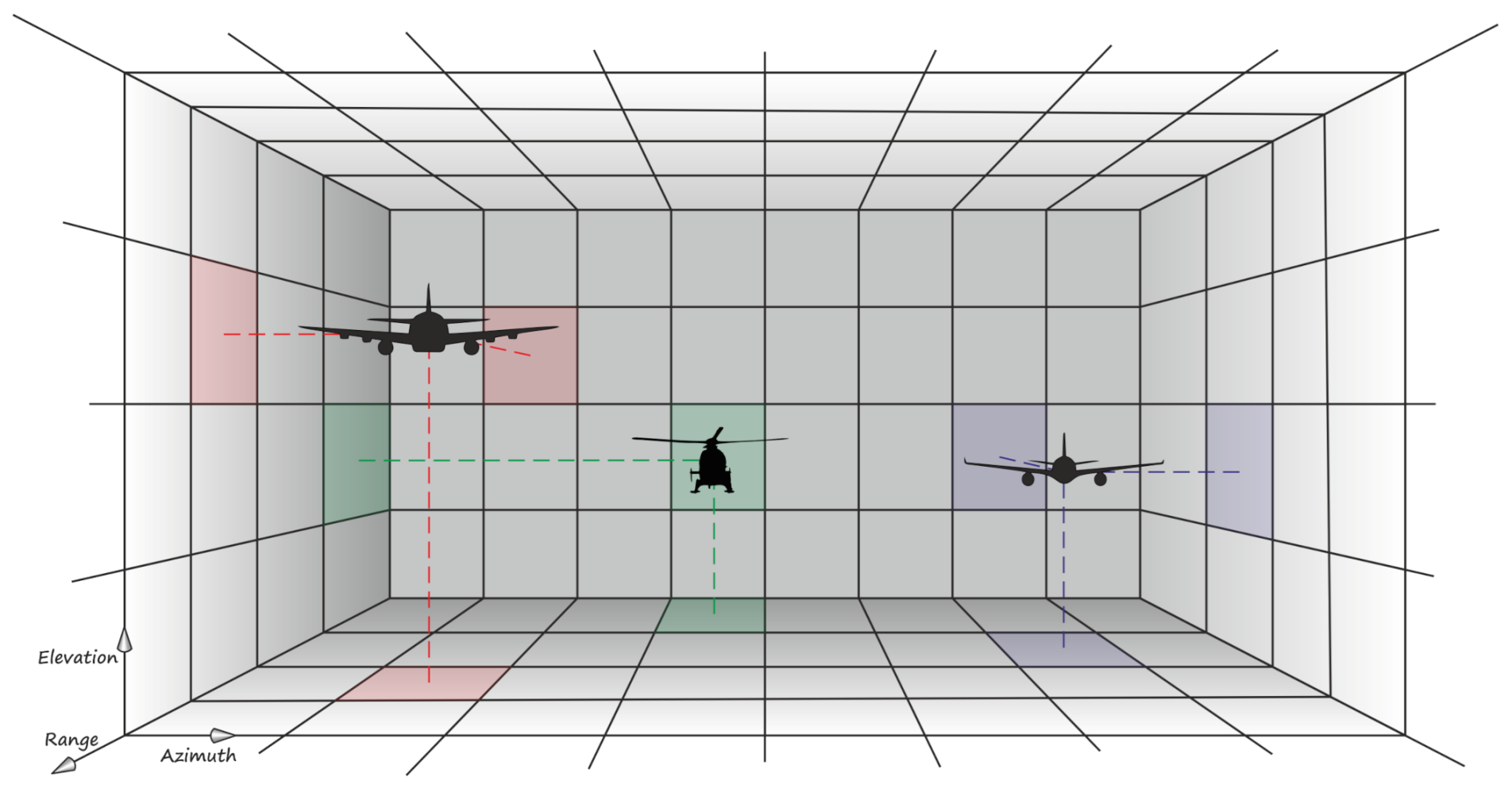
2.1. Problem Formulation
- is the set of the range bins, and indexes a discrete set of Doppler values covering the unambiguous Doppler interval;
- is a factor representative of the target response and channel effects;
- for and denote the additive interference components in the rth range bin at the mth scan, and are independent and identically distributed (iid) complex normal random vectors with zero mean and unknown positive definite Interference Covariance Matrix (ICM) ;
- is the temporal steering vector defined as:with and the prospective target radial velocity, positive if the target is approaching the radar;
- is the spatial steering vector defined as:with the fixed polar angle of target respect to the away direction. Figure 2 shows the radar geometry problem.
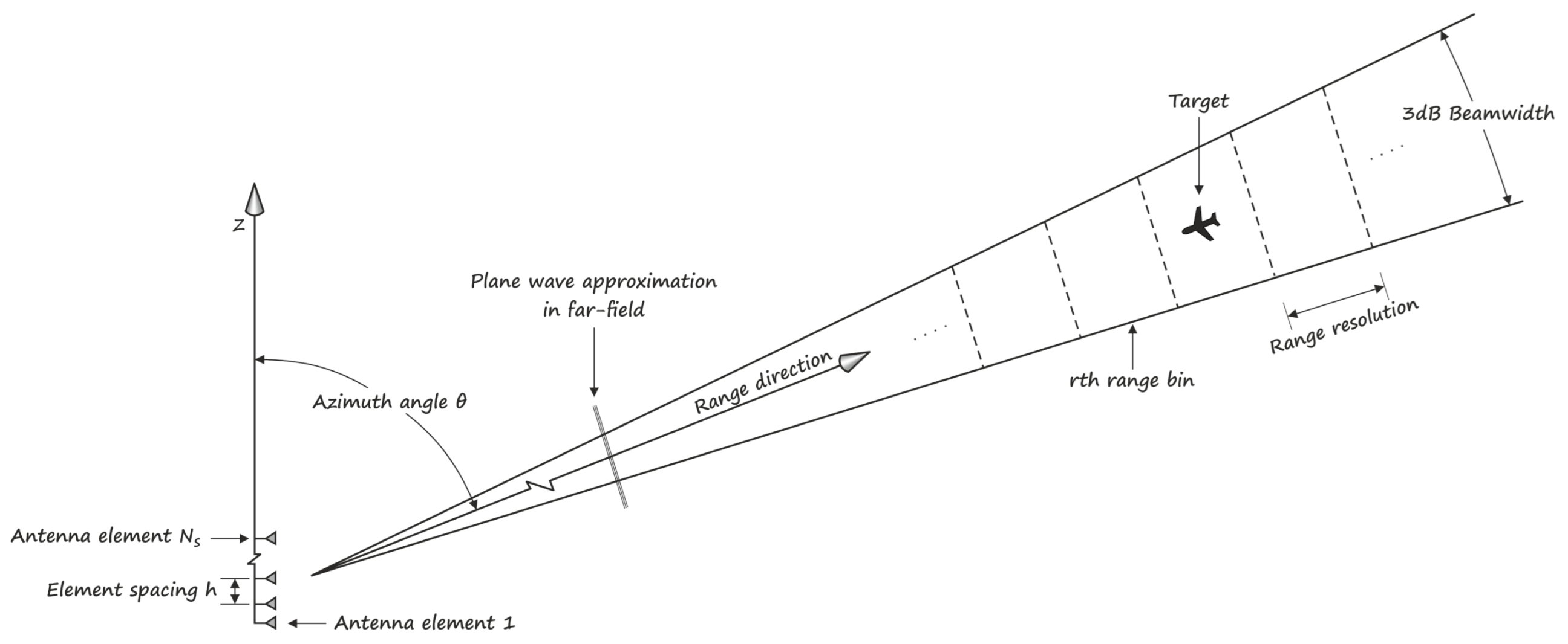
2.2. Proposed TBD Framework
2.2.1. Sparse Learning
2.2.2. Track Formation
- data assignment step: each centroid defines one cluster, therefore each vector data is assigned to its nearest centroid. This association in based on the Euclidean metric which is defined as objective function to be locally minimized:where diag is a weight matrix, represents the kth cluster centroid; stands for the assignment of the generic vector to k-cluster, and indicates the kth cluster;
- centroid update step: the centroids are recomputed by taking the mean of all vector data assigned to that cluster centroid:
2.2.3. Ad Hoc Detector
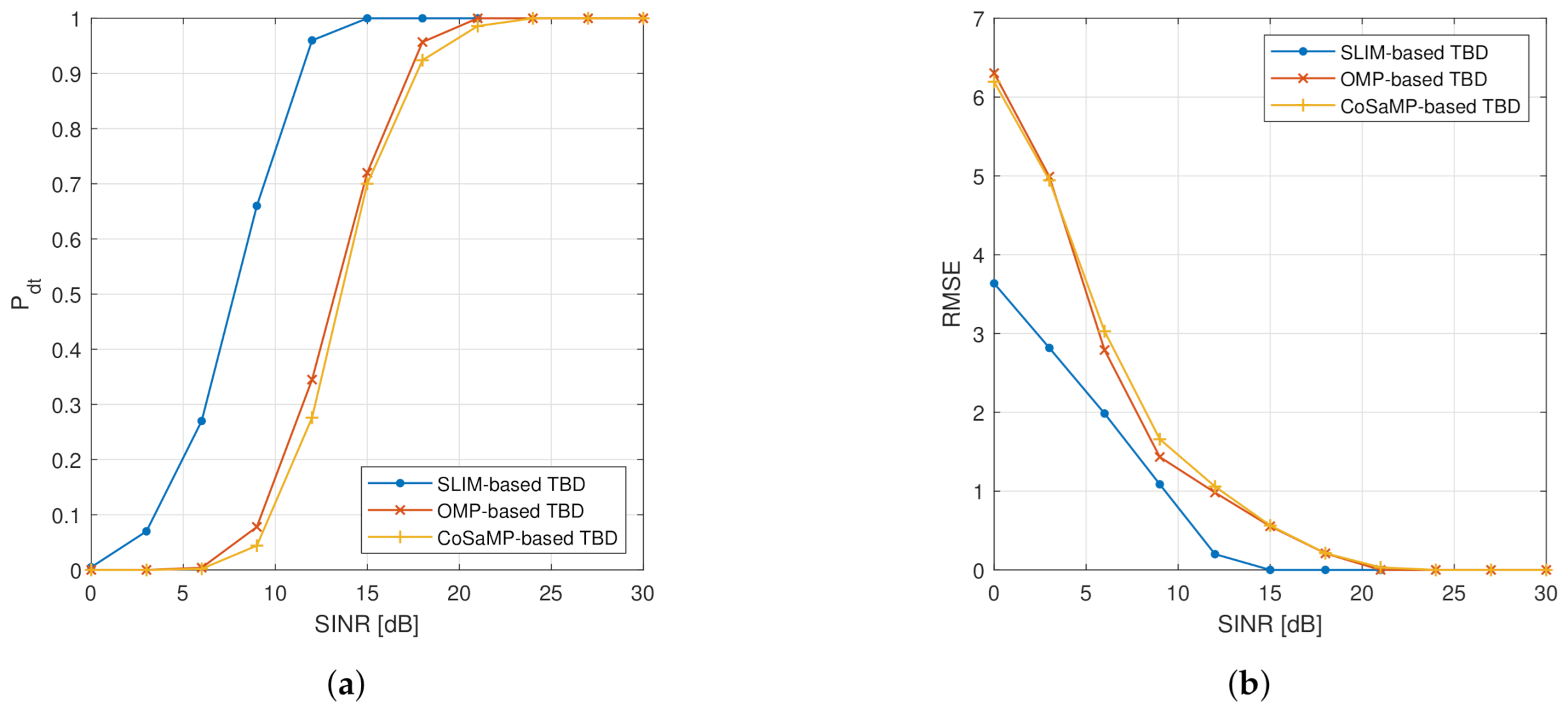
3. Results
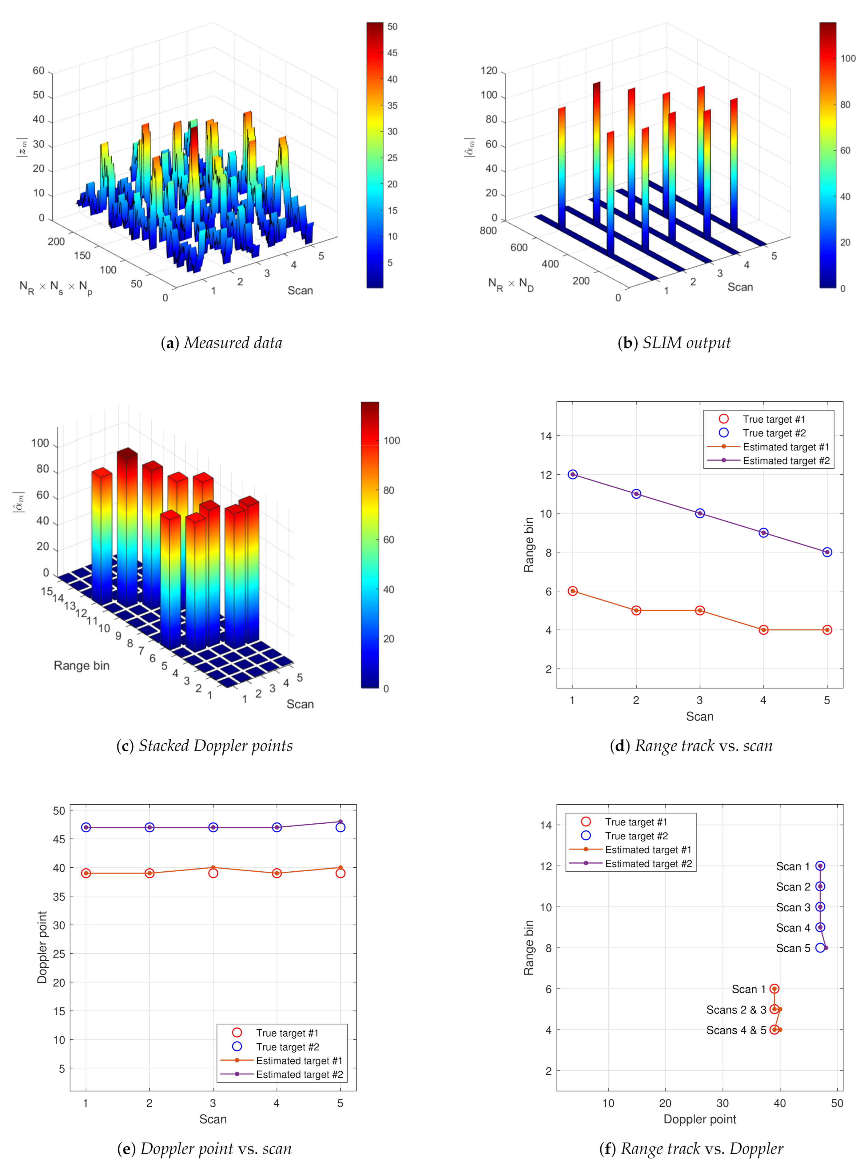
3.1. Case Study 1
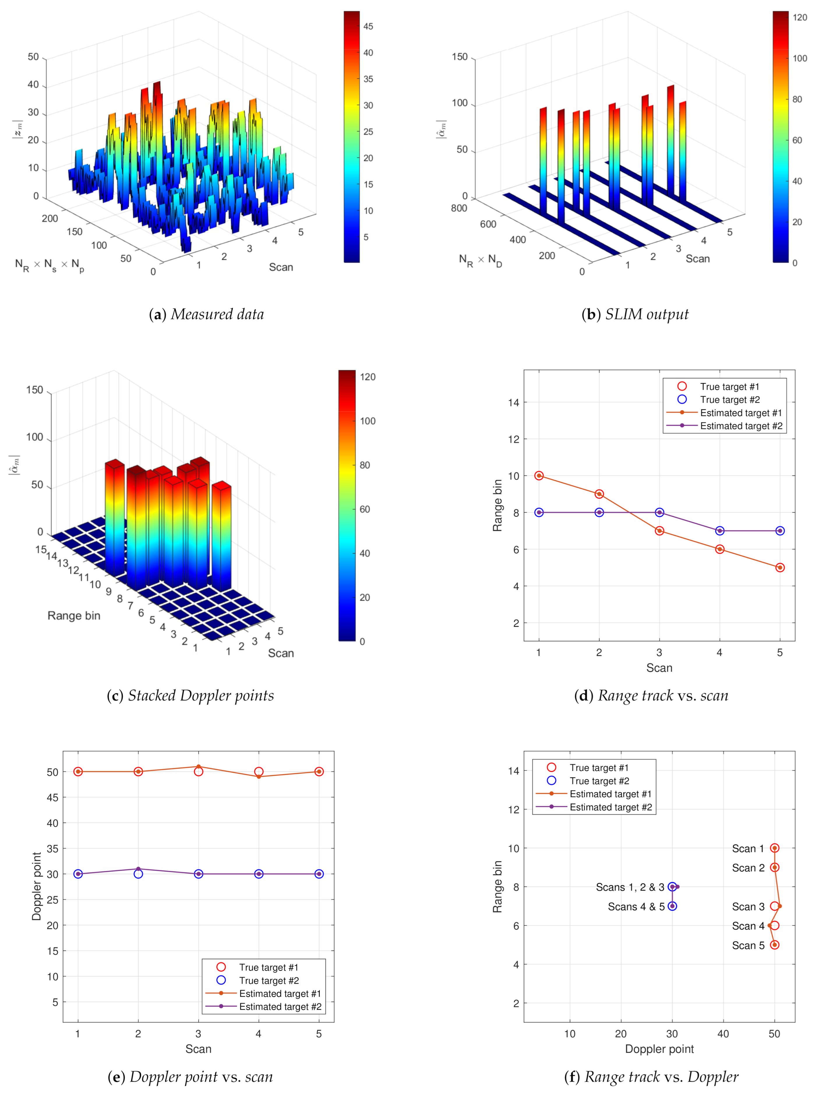
3.2. Case Study 2
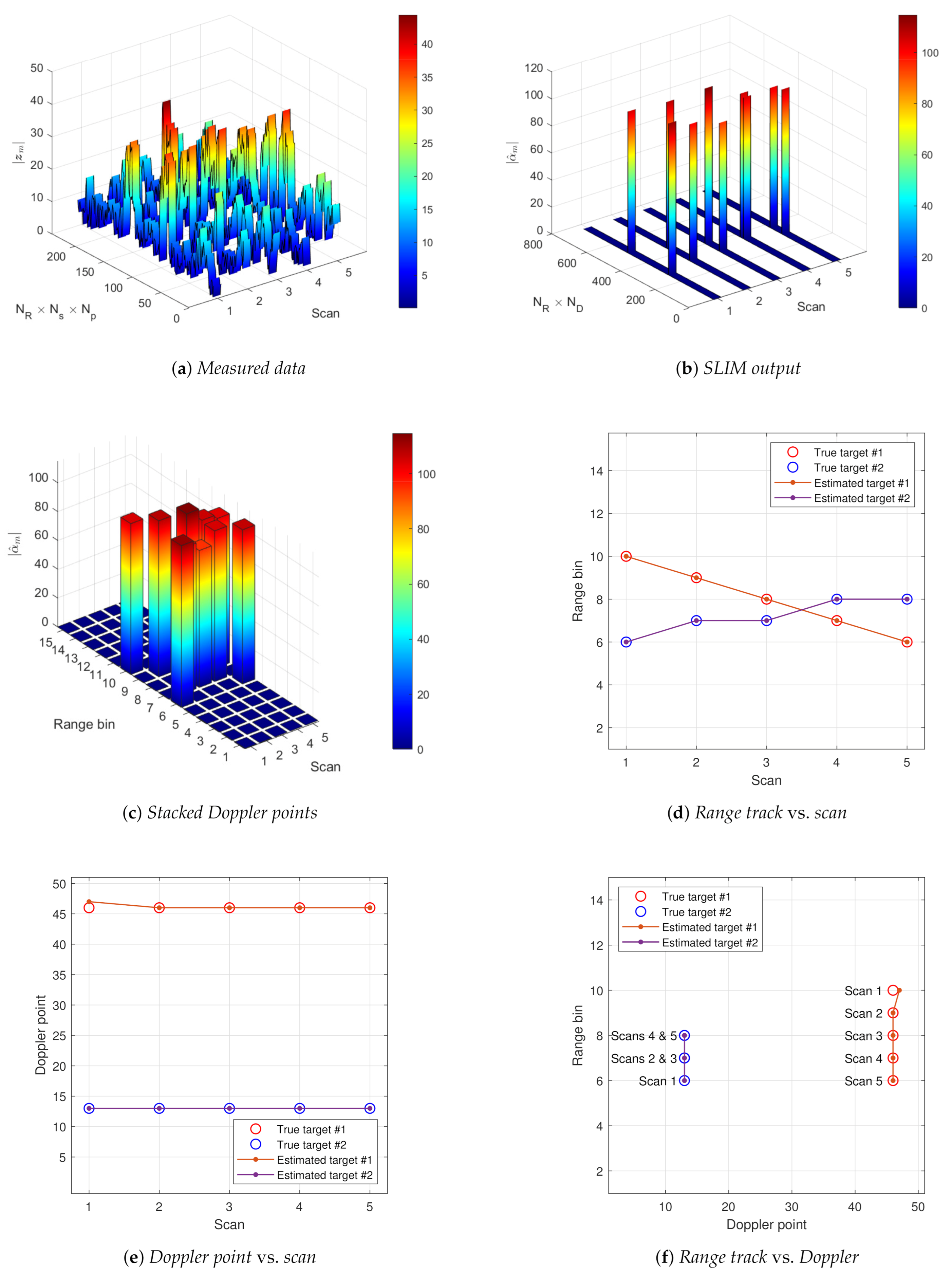
3.3. Case Study 3
4. Discussion
5. Conclusions
Author Contributions
Funding
Institutional Review Board Statement
Informed Consent Statement
Data Availability Statement
Conflicts of Interest
Abbreviations
| CoSaMP | Compressive Sensing Matching Pursuit |
| ICM | Interference Covariance Matrix |
| iid | independent and identically distribuired |
| LRT | Likelihood Ratio Test |
| OMP | Orthogonal Matching Pursuit |
| SINR | Signal to Interference plus Noise ratio |
| SLIM | Sparse Learning via Iterative Minimization |
| PRF | Pulse Repetition Frequency |
| PRI | Pulse Repetition Interval |
| RMSE | Root Mean Square Error |
| SRT | Scan Repetition Time |
| TBD | Track-Before-Detect |
References
- Mahler, R.P.S. Statistical Multisource-Multitarget Information Fusion; Artech House, Inc.: Norwood, MA, USA, 2007. [Google Scholar]
- Bar-Shalom, Y. Tracking and Data Association; Academic Press Professional, Inc.: Cambridge, MA, USA, 1987. [Google Scholar]
- Skolnik, M.I. Introduction to Radar Systems, 2nd ed.; McGraw Hill Book Co.: New York, NY, USA, 1980. [Google Scholar]
- Blackman, S.S. Multiple-Target Tracking with Radar Applications; Dedham: Andover, MA, USA, 1986. [Google Scholar]
- Kramer, J.D.R.; Reid, W.S. Track-before-detect processing for an airborne type radar. In Proceedings of the IEEE International Conference on Radar, Arlington, VA, USA, 7–10 May 1990; pp. 422–427. [Google Scholar] [CrossRef]
- Ristic, B.; Arulampalm, S.; Gordon, N. Beyond the Kalman Filter: Particle Filters for Tracking Applications; Artech House: Norwood, MA, USA, 2004. [Google Scholar]
- Barniv, Y.; Bar-Shalom, Y. Dynamic programming algorithm for detecting dim moving targets. In Multitarget-Multisensor Tracking: Advanced Applications; Bar-Shalom, Y., Ed.; Artech House: Norwood, MA, USA, 1990; Chapter 4. [Google Scholar]
- Hyoungjun, I.; Taejeong, K. Optimization of multiframe target detection schemes. IEEE Trans. Aerosp. Electron. Syst. 1999, 35, 176–187. [Google Scholar] [CrossRef]
- Johnston, L.A.; Krishnamurthy, V. Performance analysis of a dynamic programming track before detect algorithm. IEEE Trans. Aerosp. Electron. Syst. 2002, 38, 228–242. [Google Scholar] [CrossRef]
- Pohlig, S.C. An algorithm for detection of moving optical targets. IEEE Trans. Aerosp. Electron. Syst. 1989, 25, 56–63. [Google Scholar] [CrossRef]
- Tonissen, S.M.; Bar-Shalom, Y. Maximum likelihood track-before-detect with fluctuating target amplitude. IEEE Trans. Aerosp. Electron. Syst. 1998, 34, 796–809. [Google Scholar] [CrossRef]
- Davey, S.J.; Rutten, M.G.; Cheung, B. A comparison of detection performance for several Track-Before-Detect algorithms. In Proceedings of the 2008 11th International Conference on Information Fusion, Cologne, Germany, 30 June–3 July 2008; pp. 1–8. [Google Scholar]
- Salmond, D.J.; Birch, H. A particle filter for track-before-detect. In Proceedings of the 2001 American Control Conference (Cat. No.01CH37148), Arlington, VA, USA, 25–27 June 2001; Volume 5, pp. 3755–3760. [Google Scholar]
- Boers, Y.; Driessen, J.N. Particle filter based detection for tracking. In Proceedings of the 2001 American Control Conference (Cat. No.01CH37148), Arlington, VA, USA, 25–27 June 2001; Volume 6, pp. 4393–4397. [Google Scholar]
- Fallon, M.F.; Godsill, S. Acoustic Source Localization and Tracking Using Track Before Detect. Trans. Audio Speech Lang. Proc. 2010, 18, 1228–1242. [Google Scholar] [CrossRef] [Green Version]
- Boers, Y.; Driessen, H. Particle filter track-before-detect application using inequality constraints. IEEE Trans. Aerosp. Electron. Syst. 2005, 41, 1483–1489. [Google Scholar]
- Saha, S.; Boers, Y.; Driessen, H.; Mandal, P.K.; Bagchi, A. Particle based MAP state estimation: A comparison. In Proceedings of the 2009 12th International Conference on Information Fusion, Seattle, WA, USA, 6–9 July 2009; pp. 278–283. [Google Scholar]
- Vo, B.; Vo, B.; Pham, N.; Suter, D. Joint Detection and Estimation of Multiple Objects From Image Observations. IEEE Trans. Signal Process. 2010, 58, 5129–5141. [Google Scholar] [CrossRef]
- Wong, J.; Vo, B.T.; Vo, B.N.; Hoseinnezhad, R. Multi-Bernoulli based track-before-detect with road constraints. In Proceedings of the 2012 15th International Conference on Information Fusion, Singapore, 9–12 July 2012; pp. 840–846. [Google Scholar]
- Jevtić, M.; Marković, K.; Mikluc, D.; Mišić, B.; Pajić, T. Real-time implementation of target tracking system for air surveillance radar applications. In Proceedings of the 2013 11th International Conference on Telecommunications in Modern Satellite, Cable and Broadcasting Services (TELSIKS), Niš, Serbia, 16–19 October 2013; Volume 2, pp. 557–560. [Google Scholar]
- Buzzi, S.; Lops, M.; Venturino, L. Track-before-detect procedures for early detection of moving target from airborne radars. IEEE Trans. Aerosp. Electron. Syst. 2005, 41, 937–954. [Google Scholar] [CrossRef]
- Orlando, D.; Venturino, L.; Lops, M.; Ricci, G. Track-Before-Detect Strategies for STAP Radars. IEEE Trans. Signal Process. 2010, 58, 933–938. [Google Scholar] [CrossRef]
- Orlando, D.; Ricci, G.; Bar-Shalom, Y. Track-Before-Detect Algorithms for Targets with Kinematic Constraints. IEEE Trans. Aerosp. Electron. Syst. 2011, 47, 1837–1849. [Google Scholar] [CrossRef]
- McDonald, M.; Balaji, B. Impact of Measurement Model Mismatch on Nonlinear Track-Before-Detect Performance for Maritime RADAR Surveillance. IEEE J. Ocean. Eng. 2011, 36, 602–614. [Google Scholar] [CrossRef]
- Herman, M.A.; Strohmer, T. High-Resolution Radar via Compressed Sensing. Trans. Sig. Proc. 2009, 57, 2275–2284. [Google Scholar] [CrossRef] [Green Version]
- Candes, E.J.; Tao, T. Near-Optimal Signal Recovery From Random Projections: Universal Encoding Strategies? IEEE Trans. Inf. Theory 2006, 52, 5406–5425. [Google Scholar] [CrossRef] [Green Version]
- Candes, E.; Wakin, M. An Introduction To Compressive Sampling. IEEE Signal Process. Mag. 2008, 25, 21–30. [Google Scholar] [CrossRef]
- Donoho, D.L. Compressed sensing. IEEE Trans. Inf. Theory 2006, 52, 1289–1306. [Google Scholar] [CrossRef]
- Baraniuk, R.; Steeghs, P. Compressive Radar Imaging. In Proceedings of the 2007 IEEE Radar Conference, Waltham, MA, USA, 17–20 April 2007; pp. 128–133. [Google Scholar]
- Liu, Z.; Wei, X.Z.; Li, X. Adaptive clutter suppression for airborne random pulse repetition interval radar based on compressed sensing. Prog. Electromagn. Res. 2012, 128, 291–311. [Google Scholar] [CrossRef] [Green Version]
- Yang, M.; Zhang, G. Compressive Sensing Based Parameter Estimation for Monostatic MIMO Noise Radar. Prog. Electromagn. Res. Lett. 2012, 30, 133–143. [Google Scholar] [CrossRef] [Green Version]
- Grossi, E.; Lops, M.; Venturino, L. A track-before-detect procedure for sparse data. In Proceedings of the 2012 IEEE Statistical Signal Processing Workshop (SSP), Arbor, MI, USA, 4–7 August 2012; pp. 772–775. [Google Scholar]
- Liu, J.; ChongZhao, H.; XiangHua, Y.; Feng, L. Compressed Sensing Based Track before Detect Algorithm for Airborne Radars. Prog. Electromagn. Res. 2013, 138, 433–451. [Google Scholar] [CrossRef] [Green Version]
- Liu, J.; Li, X.; Xu, S.; Zhuang, Z. ISAR Imaging of Non-Uniform Rotation Targets with Limited Pulses via Compressed Sensing. Prog. Electromagn. Res. B 2012, 41, 285–305. [Google Scholar] [CrossRef] [Green Version]
- Wei, S.J.; Zhang, X.L.; Jun, S.; Liao, K.F. Sparse array microwave 3-D imaging: Compressed sensing recovery and experimental study. Prog. Electromagn. Res. 2013, 135, 161–181. [Google Scholar] [CrossRef] [Green Version]
- Li, J.; Zhang, S.; Chang, J. Applications of compressed sensing for multiple transmitters multiple azimuth beams SAR imaging. Prog. Electromagn. Res. 2012, 127, 259–275. [Google Scholar] [CrossRef] [Green Version]
- Chen, J.; Gao, J.; Zhu, Y.; Yang, W.; Wang, P. A novel image formation algorithm for high-resolution wide-swath spaceborne SAR using compressed sensing on azimuth displacement phase center antenna. Prog. Electromagn. Res. 2012, 125, 527–543. [Google Scholar] [CrossRef] [Green Version]
- Wei, S.J.; Zhang, X.L.; Jun, S. Linear array SAR imaging via compressed sensing. Prog. Electromagn. Res. 2011, 117, 299–319. [Google Scholar] [CrossRef] [Green Version]
- Wei, S.J.; Zhang, X.L.; Jun, S.; Xiang, G. Sparse reconstruction for SAR imaging based on compressed sensing. Prog. Electromagn. Res. 2010, 109, 63–81. [Google Scholar] [CrossRef] [Green Version]
- Tan, X.; Roberts, W.; Li, J.; Stoica, P. Sparse Learning via Iterative Minimization With Application to MIMO Radar Imaging. IEEE Trans. Signal Process. 2011, 59, 1088–1101. [Google Scholar] [CrossRef]
- Addabbo, P.; Aubry, A.; De Maio, A.; Pallotta, L.; Ullo, S.L. HRR profile estimation using SLIM. IET Radar Sonar Navig. 2019, 13, 512–521. [Google Scholar] [CrossRef]
- Yan, L.; Addabbo, P.; Hao, C.; Orlando, D.; Farina, A. New ECCM Techniques Against Noiselike and/or Coherent Interferers. IEEE Trans. Aerosp. Electron. Syst. 2020, 56, 1172–1188. [Google Scholar] [CrossRef] [Green Version]
- Tropp, J.A.; Gilbert, A.C. Signal Recovery From Random Measurements Via Orthogonal Matching Pursuit. IEEE Trans. Inf. Theory 2007, 53, 4655–4666. [Google Scholar] [CrossRef] [Green Version]
- Needell, D.; Tropp, J. CoSaMP: Iterative signal recovery from incomplete and inaccurate samples. Appl. Comput. Harmon. Anal. 2009, 26, 301–321. [Google Scholar] [CrossRef] [Green Version]
- Galati, G.; Mazzenga, F.; Naldi, M. Elementi di Sistemi Radar; Aracne: Rome, Italy, 1996. [Google Scholar]
- Gelman, A.; Carlin, J.B.; Stern, H.S.; Rubin, D.B. Bayesian Data Analysis, 2nd ed.; Chapman and Hall/CRC: Boca Raton, FL, USA, 2004. [Google Scholar]
- Robert, C.P.; Casella, G. Monte Carlo Statistical Methods (Springer Texts in Statistics); Springer: Berlin/Heidelberg, Germany, 2005. [Google Scholar]
- Stoica, P.; Selen, Y. Model-order selection: A review of information criterion rules. IEEE Signal Process. Mag. 2004, 21, 36–47. [Google Scholar] [CrossRef]
- Lloyd, S. Least squares quantization in PCM. IEEE Trans. Inf. Theory 1982, 28, 129–137. [Google Scholar] [CrossRef]
- MacQueen, J. Some Methods for Classification and Analysis of Multivariate Observations. In Proceedings of the 5th Berkeley Symposium on Mathematical Statistics and Probability; Le Cam, L.M., Neyman, J., Eds.; University of California Press: Berkeley, CA, USA, 1967; Volume 1, pp. 281–297. [Google Scholar]
- Ball, G.H.; Hall, D. A clustering technique for summarizing multivariate data. Behav. Sci. 1967, 12, 153–155. [Google Scholar] [CrossRef] [PubMed]
- Lockheed Martin Corporation. AN/FPS-117 Long-Range Air Surveillance Radars; Technical Report; Lockheed Martin Corporation: Washington, DC, USA, 2013. [Google Scholar]
- Bartolic, J. Near Field Measurements of the FPS-117 Solid-State Phased Array Antenna (Part I)-Self-Oscillating Antennas and Arrays (Part II). Available online: https://www.researchgate.net/publication/305969338 (accessed on 11 January 2021).
- Karakuş, C.; Gürbüz, A.C. Comparison of iterative sparse recovery algorithms. In Proceedings of the 2011 IEEE 19th Signal Processing and Communications Applications Conference (SIU), Antalya, Turkey, 20–22 April 2011; pp. 857–860. [Google Scholar] [CrossRef]


| Parameter | Value |
|---|---|
| Number of antenna sensors () | 4 |
| Antennas inter-element spacing (h) | |
| Number of pulses () | 4 |
| Carrier frequency () | 1.388 GHz |
| Pulse Repetition Frequency (PRF) | 917 Hz |
| Number of range bins () | 15, 12 |
| Range spatial resolution () | 30 m |
| Doppler interval | PRF |
| Number of Doppler points () | 51, 25 |
| Azimuth view angle () | |
| Number of targets (L) | 2 |
| Maximum radial target velocity | 49.5 m/s |
| SLIM convergence threshold () | |
| Maximum SLIM iterations | 25 |
| k-means convergence threshold () | |
| Number of radar scans (M) | 5, 4 |
| Scan Repetition Time (SRT) | 0.68 s |
| Indipendent Monte Carlo trials (n) | 1000 |
Publisher’s Note: MDPI stays neutral with regard to jurisdictional claims in published maps and institutional affiliations. |
© 2021 by the authors. Licensee MDPI, Basel, Switzerland. This article is an open access article distributed under the terms and conditions of the Creative Commons Attribution (CC BY) license (http://creativecommons.org/licenses/by/4.0/).
Share and Cite
Fiscante, N.; Addabbo, P.; Clemente, C.; Biondi, F.; Giunta, G.; Orlando, D. A Track-Before-Detect Strategy Based on Sparse Data Processing for Air Surveillance Radar Applications. Remote Sens. 2021, 13, 662. https://doi.org/10.3390/rs13040662
Fiscante N, Addabbo P, Clemente C, Biondi F, Giunta G, Orlando D. A Track-Before-Detect Strategy Based on Sparse Data Processing for Air Surveillance Radar Applications. Remote Sensing. 2021; 13(4):662. https://doi.org/10.3390/rs13040662
Chicago/Turabian StyleFiscante, Nicomino, Pia Addabbo, Carmine Clemente, Filippo Biondi, Gaetano Giunta, and Danilo Orlando. 2021. "A Track-Before-Detect Strategy Based on Sparse Data Processing for Air Surveillance Radar Applications" Remote Sensing 13, no. 4: 662. https://doi.org/10.3390/rs13040662