Downscaling Snow Depth Mapping by Fusion of Microwave and Optical Remote-Sensing Data Based on Deep Learning

Abstract

Accurate high spatial resolution snow depth mapping in arid and semi-arid regions is of great importance for snow disaster assessment and hydrological modeling. However, due to the complex topography and low spatial-resolution microwave remote-sensing data, the existing snow depth datasets have large errors and uncertainty, and actual spatiotemporal heterogeneity of snow depth cannot be effectively detected. This paper proposed a deep learning approach based on downscaling snow depth retrieval by fusion of satellite remote-sensing data with multiple spatial scales and diverse characteristics. The (Fengyun-3 Microwave Radiation Imager) FY-3 MWRI data were downscaled to 500 m resolution to match Moderate-resolution Imaging Spectroradiometer (MODIS) snow cover, meteorological and geographic data. A deep neural network was constructed to capture detailed spectral and radiation signals and trained to retrieve the higher spatial resolution snow depth from the aforementioned input data and ground observation. Verified by in situ measurements, downscaled snow depth has the lowest root mean square error (RMSE) and mean absolute error (MAE) (8.16 cm, 4.73 cm respectively) among Environmental and Ecological Science Data Center for West China Snow Depth (WESTDC_SD, 9.38 cm and 5.36 cm), the Microwave Radiation Imager (MWRI) Ascend Snow Depth (MWRI_A_SD, 9.45 cm and 5.49 cm) and MWRI Descend Snow Depth (MWRI_D_SD, 10.55 cm and 6.13 cm) in the study area. Meanwhile, downscaled snow depth could provide more detailed information in spatial distribution, which has been used to analyze the decrease of retrieval accuracy by various topography factors.

1. Introduction

Snow is an important indicator for global climate change, which has significant positive and noteworthy negative feedbacks on climate system, water resources and ecological environment [1,2,3,4]. On the positive side, due to the high surface albedo and large-scale cooling effect, snow cover (SC) participates in energy exchange between the atmosphere and Earth’s land, thus regulating regional and global climate. Snowmelt can provide water resources for ecosystem and participate in regional water cycles, which is beneficial for arid and semi-arid region. Meanwhile, snow water equivalent (SWE) is an important driving factor for meteorological, climate and hydrological models, which can enhance the understanding of regional water resources environment and improve the accuracy of a weather forecast. From a negative perspective, heavy snow, sustained low temperatures and prolonged SC will result in snow disasters that affect animal husbandry, and sudden excessive snow melting will also cause soil erosion and flood risk [5].

As the most sensitive and active response to climate change, snow has become an important field of research. Currently, snow cover mapping using optical remote sensing has developed many mature datasets, such as Landsat [6], Systeme Probatoire d’Observation de la Terre (SPOT) [7], Advanced Very High Resolution Radiometer (AVHRR) [8] and Moderate-resolution Imaging Spectroradiometer (MODIS) snow cover datasets [9,10,11,12,13]. MODIS carried by Terra and Aqua satellites, is the most deeply studied and widely applied. The high spectral and spatial resolution characteristics of the sensor provide favorable conditions for the exploration and research of snow cover extraction. However, due to the similar reflectance spectrum characteristics of snow and cloud, optical remote-sensing monitoring of snow cover is greatly limited by weather conditions. Simultaneously, snow depth is hardly detected by optical sensors. Passive microwave can penetrate cloud layers for all-weather work, and achieve the parameter of snow depth through the surface based on the sensitivity of different snow frequency.

Passive microwave remote-sensing data are mainly used for monitoring snow depth and SWE at a global or hemispherical scale. To date, the existing space-borne passive microwave sensors are the Scanning Multichannel Microwave Radiometer (SMMR) on Nimbus-7, Special Sensor Microwave Imager (SSM/I) [14] and Special Sensor Microwave Imager/Sounder (SSMI/S) on the Defense Meteorological Satellite Program (DMSP), the Advanced Microwave Scanning Radiometer-EOS (AMSR-E) on the Aqua satellite, the Advanced Microwave Scanning Radiometer 2 (AMSR-2) on the Global Change Observation Mission–Water (GCOM-W1) satellite, and the Microwave Radiation Imager (MWRI) on Fengyun-3 (FY-3) series satellites. Many methods for retrieving snow depth and SWE using passive microwave brightness temperature (BT) data have been proposed and developed [15].

The widely used Chang’s algorithm [16] uses radiation transfer model simulation results and ground station observation data for linear regression analysis, and finally obtains the linear relationship between snow depth and brightness temperature difference (BTD) of 18 GHz and 36 GHz horizontal polarization. Similarly, the spectral polarization difference (SPD) algorithm proposed by Aschbacher [17] is based on BTD between horizontal and vertical polarization at 19 GHz and 37 GHz. Given the difference between snow characteristics in China and North America, Che [18] revised the retrieval coefficients applicable to China based on Chang’s algorithm. Due to the influence of forest, water body, elevation and topography on snow attributes, many researchers introduced parameters such as forest coverage fraction and land-cover types to modify the coefficients of snow depth retrieval algorithm to improve the accuracy [2,19,20]. Based on the abovementioned algorithms, many scholars have improved the algorithm by considering the influence of snow physical properties on microwave emission characteristics. The temperature gradient index (TGI) is used to describe the cumulative effect of temperature gradient on snow layer, and then calculate snow depth [21]. However, the result shows that the method has high accuracy only in the North American plain. Kelly used Dense media radial transfer (DMRT) to simulate the change of snow particle size and density and integrates the influence of snow attribute changes on BT in the retrieval process [22]. However, these algorithms have poor applicability. The radiative transfer model of snow cover can simulate the radiative transfer process of microwave in the snow layer and detect the parameters of snow [23,24]. However, these models simplify the radiative transfer of snow, and the detailed parameters in the models are difficult to obtain. The static factors that affect the distribution of snow and dynamic factors affecting the snow melting have been considered and calculated, and the retrieval model of snow depth has been improved continuously.

Machine-learning and deep-learning technology power many aspects of remote sensing: from target recognition [25,26,27,28,29] to semantic segmentation [30,31] to spatial-temporal prediction [32,33], and they are increasingly present in snow parameter estimation and retrieval [34,35,36]. Tedesco [37] constructed a neural network to retrieve the snow depth and SWE, which showed the highest accuracy compared with the other four retrieval algorithms. Tabari [38] achieved the similar conclusion by using a neural network to estimate snow depth and SWE in the Samsami Basin, Iran. Theoretically speaking, microwave BTD enhances with the increases of snow depth, but when the snow depth exceeds a certain threshold (50 cm) there will be a large error in the estimation results. The neural network could overcome various complex problems existing in large-scale retrievals, such as non-linear modeling, classification and association by learning and summarizing a large number of data and does not rely on the understanding of physical process when modeling. The support vector machine (SVM) is also widely used to solve the nonlinear problems in geosciences. Xue [34] reveals that SVM is more sensitive than the neural network in estimating snow parameters. It has been found that the results based on the SVM algorithm have better accuracy no matter in deep or shallow snow cover, forest coverage area, snow accumulation and melting period. Xiao [39] used the support vector regression (SVR) algorithm to establish a snow depth retrieval model based on different vegetation types and different snow periods, showing better accuracy and reducing "snow saturation effect". Machine learning and deep learning technology can describe the non-linear relationship between BTD and snow parameters, and overcome the limitations of a linear algorithm in different areas [40,41]. Although the machine learning technology has a wide range of applications and high accuracy, there is no detailed snow physical model involved in the retrieval process [42], thus the interpretability of the results is poor.

The model of retrieving snow depth from microwave data has developed from simple linear regression to non-linear models considering complex meteorological and geographical factors. However, the snow depth with spatial resolution from 10 km to 25 km is not suitable for arid and semi-arid alpine region where the vertical drop is extremely significant. In practical application, snow depth mapping with higher spatial resolution is more useful for regional snow disaster evaluation and hydrological model establishment. Recent studies have demonstrated that higher snow depth mapping can be developed based on high-resolution geographic and meteorological data, together with downscaling microwave data. Wang developed a multifactor power snow depth downscaling model and greatly improved accuracy of snow depth retrieval [43]. Walters [44] describes and tests a linear model to downscale MOD10A1 fractional snow cover area (fSCA) (500 m) data to higher-resolution (30 m) spatially explicit binary snow cover area (SCA) estimates. Mhawej [45] downscaled Advanced Microwave Scanning Radiometer – Earth Observing System snow water equivalent (AMSR_E SWE) datasets based on the cooperative observation of MODIS Terra-Aqua data. For the arid and semi-arid alpine regions such as Northern Xinjiang (NX) with complex topography and violent vertical variation, high-resolution snow depth mapping can more accurately describe the accumulation and melting of snow in the region, and provide precise input parameters for hydrological process and snow disaster early warning. Thus, in this manuscript, we propose a deep learning approach to downscale and evaluate the snow depth in NX.

This manuscript is organized as follows. After introducing the study area and data preprocessing in Section 2, the methodology for snow identification and downscaling snow depth retrieval is expounded in Section 3. Results of accuracy verification and spatial comparison will be presented in Section 4, and more details will be discussed in Section 5. Ultimately, a summary of the research will be described in Section 6.

2. Study Area and Data

2.1. Study Area

The study area for this manuscript was Northern Xinjiang (NX), located in the northwest of China, at 79.90°–96.18°E and 40.88°–48.10°N, as shown in Figure 1. The total land area is 0.97 million km², accounting for nearly 10% of China’s land area. Junggar Basin is lying between Tianshan Mountains and Altai Mountains, forming a mountain-basin system, which is the most significant landform in NX [46,47,48]. Xinjiang is far from the ocean and has a continental arid and semi-arid climate with an annual mean temperature varying from 4 to 8 °C in NX. Due to the unique geographical location and topographic factors, the variation of temperature difference in this area is very significant. Simultaneously, an inversion layer often appears due to the effect of the cold lake in winter in Junggar Basin. Data analysis reveals that the average temperature in January in this area is mostly lower than −10 °C. Another significant feature of temperature variation in this area is that the closer to the Junggar Basin, the higher the temperature is. Below the altitude of 2000 m, the temperature increases with the elevation. Vegetation is sparse in the plains and the altitudinal belts of mountains are obvious [49]. The precipitation in alpine regions can reach 400–600 mm, and exceed 800 mm in specific areas. Snowfall accounts for more than 80% of the annual precipitation. In the piedmont plain, precipitation ranges from 100 to 200 mm and less than 50 mm in a specific area, and snowfall accounts for about 1/3 of the annual precipitation. Solid precipitation is the main form of precipitation across arid alpine areas in winter. The northwest arid region is the area with extremely poor surface water resources and the most abundant snow resources in China [50]. It is one of the three stable snow regions in China, namely, the Qinghai Tibet Plateau, Tianshan-Northern Xinjiang and Northeast-Inner Mongolia. Among them, the snow resources in NX are more advantaged, accounting for 1/3 of the national snow resources. In most areas of the NX plain, the period of stable snow cover lasts about five months and the snow thickness is generally 20–50 cm. However, the stable snow period in alpine regions lengthen out to 7 months every year, and the snow thickness is greater than 80 cm, and the stable snow cover in high mountain areas accumulates all year round. Except for Irtysh River, other rivers in NX are inland rivers, many of them originate from the northern foot of Tianshan Mountains. Thus, mountain glacier and snow meltwater resources are the major supplies of surface runoff in NX, where freshwater resources are seriously scarce [51]. Snow plays a very important role in regional ecological environment change across NX.

2.2. Microwave Radiation Imager (MWRI) Brightness Temperature (BT)

MWRI was launched onboard the Fengyun 3B (FY3B) satellite, which is mainly used to detect precipitation rate, water content of cloud, water quantity, total water vapor, soil moisture, sea ice, temperature and snow cover for the research of water cycle and energy transfer at global and hemispherical scales (http://satellite.nsmc.org.cn (accessed on 1 November 2020)). The main parameters of the sensor are listed in

Table 1. Parameters of FY-3B MWRI (Microwave Radiation Imager) sensor.

Frequency (GHz)	10.65	18.7	23.8	36.5	89
Resolution (km)	51 × 85	30 × 50	27 × 45	18 × 30	9 × 15
Bandwidth (MHz)	180	200	400	900	2300
Polarization	V, H	V, H	V, H	V, H	V, H
Sensitivity (K)	0.6	1	1	1	2
Accuracy (K)	1.2	2	2	2	2.8
Angle of Incidence (°)	53
Swath (km)	≥1400

. The resolution of different frequencies ranges from 9 km to 85 km, and each frequency has two modes of vertical polarization and horizontal polarizations. The mean accuracy of sensor is 2 K, which is lower than the accuracy of 1 K of AMSR-2. The MWRI Level 1 BT data were downloaded for the snow seasons from 2011 to 2016 and were used to construct the downscaling snow depth model, data from four snow seasons (1 November 2011–31 March 2014, 1 November 2015–31 March 2016) were used to train the model, and data from 1 November 2014 to 31 March 2015 with few extreme abnormal weather were chosen to validate and evaluate model accuracy. In this manuscript, the official ascending and descending orbit snow depth datasets were denoted as MWRI_A and MWRI_D, respectively and were used to compare with the spatial distribution of downscaled snow depth.

The high-frequency and low-frequency polarimetric data of ascending and descending orbit are the main inputs to construct the downscaling snow depth model. Original BT data were resampled to 500 m resolution with nearest-neighbor interpolation to match snow cover data, meteorological and geographic data. Based on the longitude and latitude information of national meteorological stations, the pixel BT data of specific coordinates are extracted for modeling and analysis [43].

2.3. Moderate-Resolution Imaging Spectroradiometer (MODIS) Datasets (MOD10A1 and MOD35)

Downscaling snow depth retrieval not only utilizes the sensitivity of microwave data at different frequencies, but also depends on high spatial resolution snow cover pixels. In arid and semi-arid regions, clouds and snow have similar reflectance in the visible spectrum, which makes it difficult to distinguish them. Thus, the contrast in reflectance of snow between the visible spectrum and shortwave infrared spectrum was used to discriminate clouds from snow. The normalized difference snow index (NDSI) applies this contrast to discriminate snow from clouds and other surface covers in mountainous terrain [3]. The MOD10A1/MYD10A1 datasets based on this method, with 500 m resolution, have reached an accuracy of 80%. In this manuscript, MOD10A1 and MYD10A1 were used to synthesize the snow cover distribution in the study area.

The MOD10A1 V006 product, which is an improved version of V005, includes four basic data layers: the NDSI_Snow_Cover, NDSI, albedo and data quality assessment layers [52]. The subpixel of fractional snow cover with 500 m resolution is not considered in this study. Therefore, the pixel with fractional snow cover from 1% to 100% is determined as a snow pixel.

However, optical remote-sensing data can not effectively detect the ground snow information under all weather conditions and at all times, thus MOD35 and MYD35 were used to distinguish between cloudy and cloudless weather conditions. In cloudless weather, the snow cover detected by optical remote sensing is accepted, while in cloudy weather, passive microwave remote sensing data has the greatest potential to derive snow coverage.

2.4. Air Temperature

Air temperature has a significant influence on snow freezing and melting. The change of temperature will influence the content of liquid water in snow, then changes the grain size and density of snow, which will affect the detection of snow depth by satellite microwave data [53]. The air temperature used in the downscaling snow depth retrieval model was from the Global Land Data Assimilation System (GLDAS) data [54,55], GLDAS-Noah is the Noah model driven by the Global Land Data Assimilation System, version 2.1 (GLDAS-2.1) (https://disc.gsfc.nasa.gov/datasets/ (accessed on 1 November 2020)), which was developed jointly by scientists at the National Aeronautics and Space Administration (NASA) Goddard Space Flight Center (GSFC) and the National Oceanic and Atmospheric Administration (NOAA) NCEP [56]. GLDAS provides temperature data with a maximum spatial resolution of 0.25° × 0.25° and a temporal resolution of 3 h. These data are resampled and calculated into daily mean temperature of 500 m resolution to match other datasets and were fed to the model.

2.5. Land Cover

The scattering and attenuation degree of microwave emission energy of various land cover are different, which is a significant factor for retrieving snow depth [57]. The MODIS Land Cover Type (MCD12Q1) Version 6 data product provides global land cover types at yearly intervals and was selected to characterize the underlying surface coverage of the study area. MCD represents the fusion of two MODIS sensors mounted on Aqua and Terra, and its spatial resolution is 500 m. The International Geosphere-Biosphere Program (IGBP) classification system was adopted to classify land cover data into 17 categories, including Water, Permanent Wetlands, Various Forest, Shrublands, Grassland, Cropland, Urban and Built-up Lands and Barren, etc. Based on the approach of MCD12Q1 reclassification from Huang [43], the land cover in NX was reclassified into five types: Water, Forest, Grassland, Farmland and Bare land (showed in Figure 2). The aforementioned four land types account for 0.47%, 0.42%, 44.18%, 7.03% and 47.9% of the total area of NX respectively. Bare land dominates the eastern regions of NX, grassland dominates Altai Mountain and Tianshan mountain area, while cultivated land and pasture are important land-cover types in Ili River Valley.

2.6. Topographic

Topography also affects the rate of snow accumulation and melting, and has a significant effect on snow redistribution. The Shuttle Rader Topography Mission (STRM) version 004 digital elevation model (DEM) data with 90 m resolution used in this study was mapped by the U.S. Geological Survey (USGS) using interferometric radar and can be download from http://srtm.csi.cgiar.org/index.asp (accessed on 1 November 2020) [58,59]. The original DEM data were also transformed, mosaiced and extracted and resampled to 500 m spatial resolution by ArcGIS 10.1 Desktop software to match the other dataset according to the vector file of NX. The elevation data of NX is shown in Figure 1. Tianshan and Altai mountains are the two regions with the highest altitude and the most complex terrain. This study will focus on snow depth observation in the aforementioned regions.

A variety of terrain factor data derived from DEM are calculated and used as prior knowledge to represent geomorphic features. Slope is the degree of steepness and slowness of surface units, which can also significantly affect the scale and intensity of the flow and energy conversion of land cover. Furthermore, slope has an important influence on the accumulation and melting speed of snow. Aspect is defined as the projection direction of the slope normal on the horizontal plane. The slope and aspect determine the total solar radiation received by snow and then affect the snow melting speed [60]. The definition of fluctuation refers to the difference between the highest and lowest altitude in a specific area. Compared with DEM, fluctuation reflects the change of elevation difference in a pixel more accurately, which has a significant impact on snow redistribution caused by drifting snow. The surface roughness affects the surface momentum transport efficiency, and thus redistributes the snow cover [61]. The aforementioned topographic factors, with 500 m resolution, are all calculated by ArcGIS 10.1 Desktop software.

2.7. Ground Observation

To construct a retrieval model and compare the accuracy of downscaled snow depth and other reported snow depth datasets, daily ground snow depth observation data of national meteorological station obtained from National Meteorological Information Center (http://data.cma.cn/site (accessed on 1 November 2020)) were used as the objective truth value for verification. Ground observations from 1 November 2014 to 31 March 2015. were used to validate the downscaled results and observations from the other four snow seasons were used to develop the model.

2.8. Long-Term Series of Daily Snow Depth Dataset in China

A long-term series of the daily snow depth dataset developed by Che [2] was used to verify whether the spatial distribution of downscaled snow depth in this research is consistent with the widely accepted and reported snow depth datasets. Snow depth datasets were denoted as Environmental and Ecological Science Data Center for West China Snow Depth (WESTDC_SD), with 25 km spatial resolution, and the data are sorted in ASCII format. The original data used to retrieve the snow depth dataset were SMMR (1979–1987), SSM/I (1987–2009) and SSMI/S (2008–2019) daily passive microwave BT data [15,62]. The data obtained are inconsistent since three sensors are mounted on different satellite platforms. The consistency of BT data is improved by simultaneous interpreting BT of different sensors. Ultimately, snow depth was retrieved by modified Chang’s algorithm [16]. In this manuscript, the daily snow depth dataset in China from 1 November 2014 to 31 March 2015 was transformed into Geo-tiff format to evaluate and verify the downscaled snow depth.

3. Methodology

Due to the different characteristics of an optical sensor and passive microwave sensor, MODIS data of the optical sensor and MWRI data of the passive microwave radiometer have advantages and limitations in snow parameter retrieval. Generally speaking, MODIS data has a high spatial resolution. The visible and shortwave infrared bands can be used to identify snow cover effectively. However, large-scale snowfall was often accompanied by cloudy and bad weather. The strong reflection of visible and near-infrared at the cloud top will shield the ground information, resulting in the lack of snow parameters under the cloud. Also, cirrus clouds have similar spectral characteristics to snow cover in the visible band, which often leads to the misjudgment of snow cover. MWRI data can penetrate through cloud and fog, not affected by cloud layer and other factors. MWRI data has the ability to observe the ground snow information all day long and penetrate the snow layer to detect the snow depth and SWE. However, there is a large deviation in regional scale snow recognition due to the coarse spatial resolution of MWRI data.

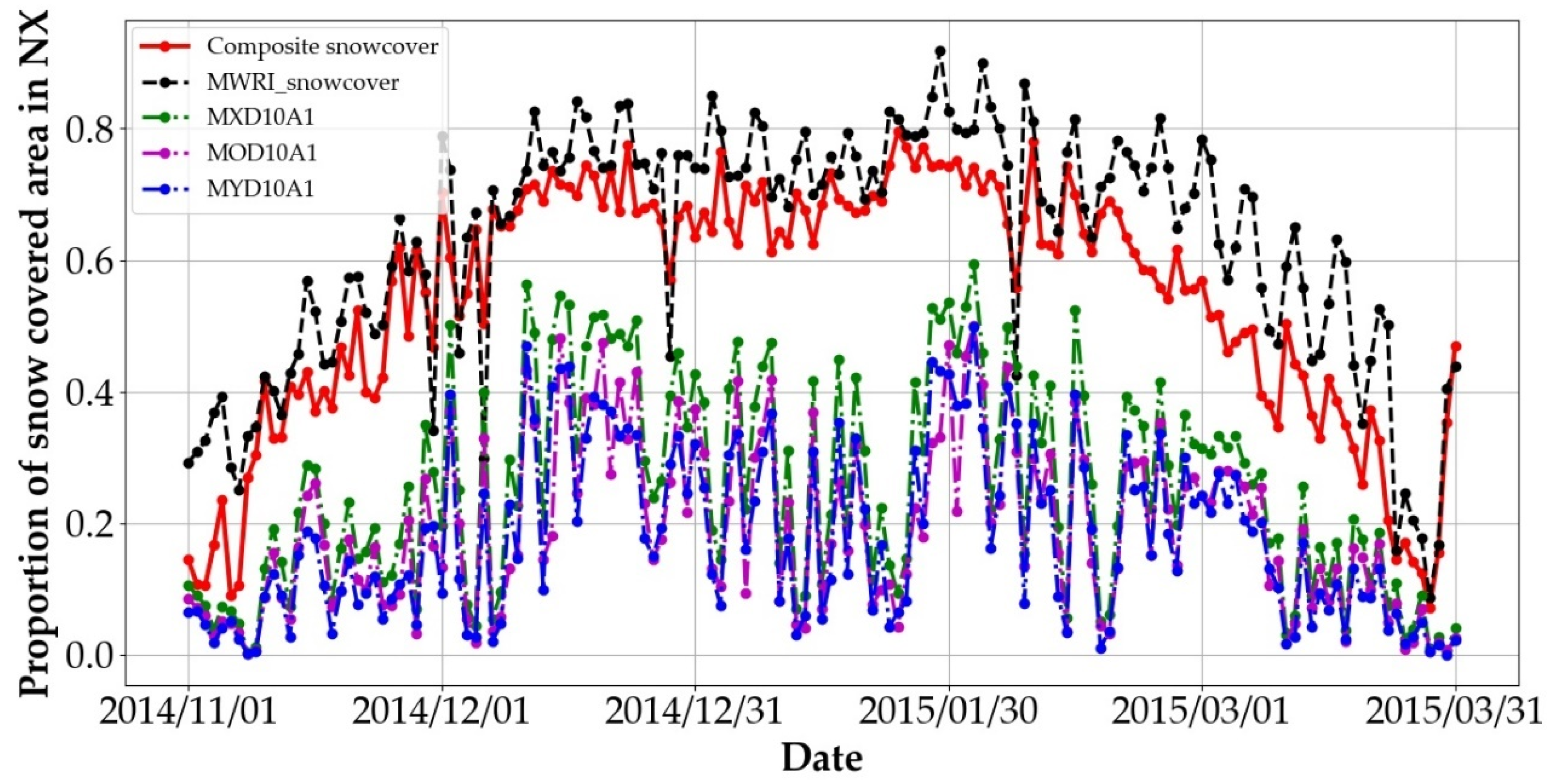
To realize the complementary advantages of the two types of data, improve the accuracy of snow identification, maxing the snow information, and obtain daily continuous snow monitoring data under all-weather conditions with and without clouds, it is imperative to effectively combine the two types of data to retrieve snow parameters.

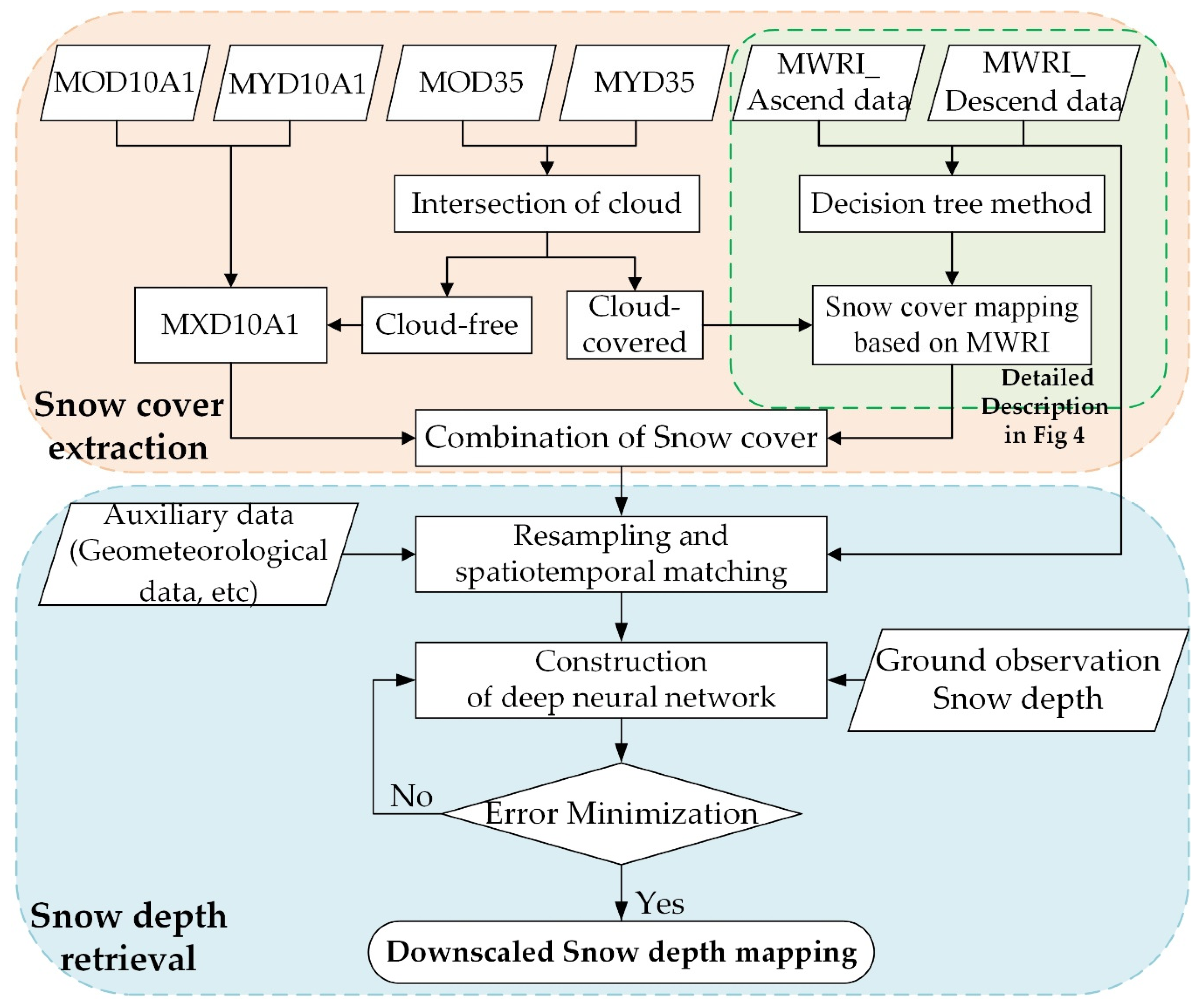
A collaborative retrieval of snow parameters based on MODIS and MWRI data is designed in this manuscript, and the technical flow chart is shown in Figure 3. The cloud will move rapidly with the wind, and its spatial position and coverage in the morning and afternoon will often change rapidly, while the snow coverage and the spatial position of the ground features are relatively fixed. Therefore, the complementary information and synthesis of the snow extent in the morning and afternoon can effectively remove the influence of cloud and restore the snow under the cloud layer. Meanwhile, the high-resolution information of the optical sensor is retained to the maximum extent. The maximum daily snow cover with 500 m resolution under all weather conditions is obtained by using optical and microwave data, high-resolution auxiliary data (DEM, Geodata, etc.) is added to the microwave data to map the snow depth. The concrete steps are as follows:

Step 1: Using the remote-sensing data MOD10A1 and MYD10A1, the daily snow cover MXD10A1 is extracted cooperatively, and the cloud interference is removed based on the dynamic of clouds;

Step 2: Extraction of snow cover under cloud-covered using MWRI data based on decision tree algorithm;

Step 3: The snow cover retrieved from MODIS and MWRI single sensor is combined to further remove the influence of cloud, MXD10A1 was adopted in cloud free conditions, while MWRI derived snow cover was adopted in cloud covered conditions, the complete snow cover information without cloud interference is thus combined and obtained;

Step 4: Preparation of input variables: Resampling and spatiotemporal matching of snow cover and auxiliary data;

Step 5: Ground observations are used as target labels to train the model and minimize errors.

3.1. Snow Cover Identification from MWRI

Nowadays, snow cover datasets widely used in investigations of climate, hydrology, and glaciology are likely derived from MODIS data, which cover the whole Earth at a near-half daily frequency through the cooperative observation of Terra and Aqua [3,4]. The combination of MOD10A1 and MYD10A1 can effectively reduce cloud interference and obtain more accurate snow cover distribution. However, the cloud layer limits the optical sensor to detect the ground snow information. In winter, the cloud layer will cover more than 50% of NX [6]. Microwave data were used to retrieve snow cover distribution under clouds.

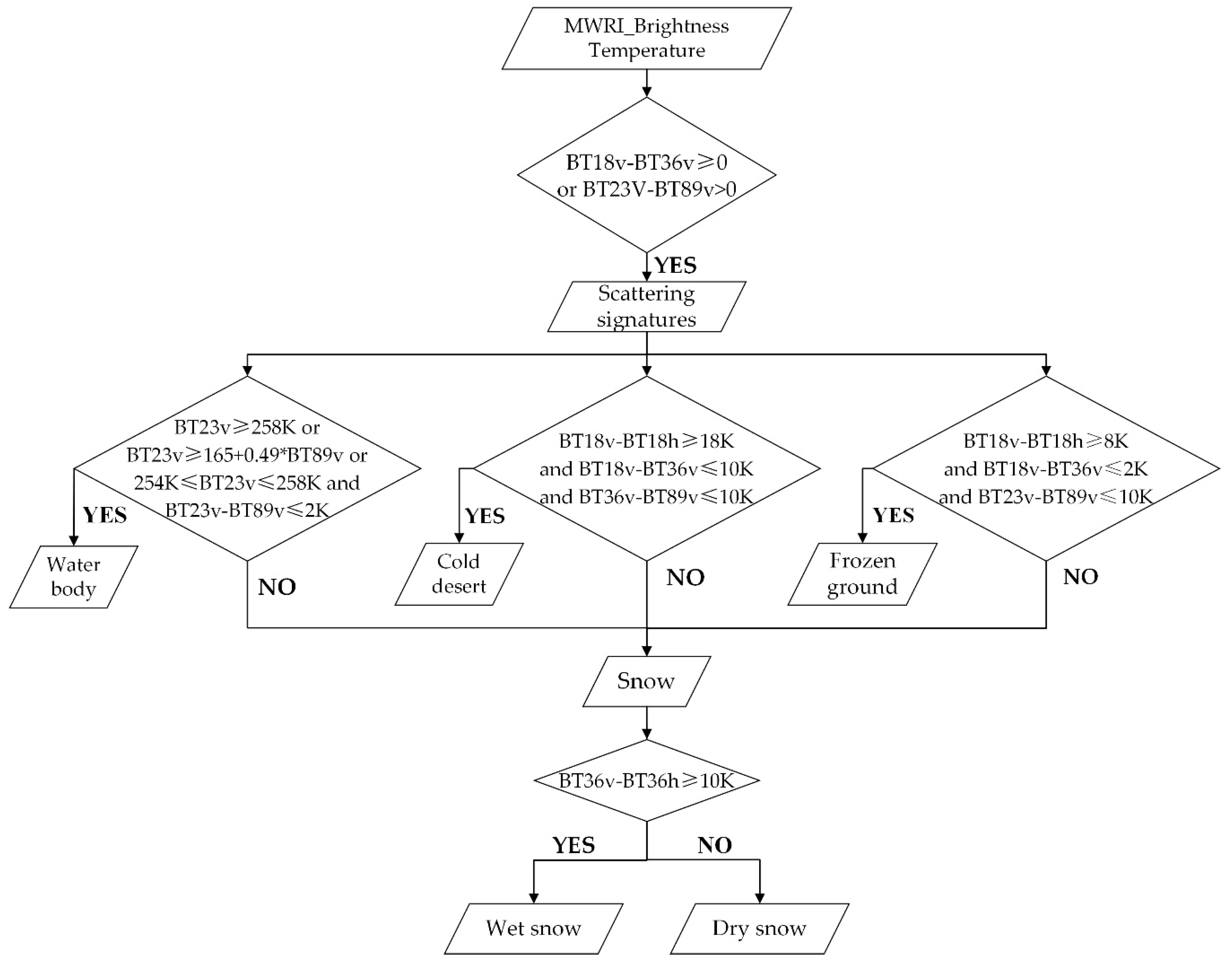
There is a large difference of polarization between snow cover and the bare surface, and the horizontal polarization is much smaller than the radiation BT of vertical polarization. With the increase of snow depth, the polarization effect of microwave radiation enhanced, the dual polarization BT of different frequencies tends to be consistent and there is free snow cover. In arid and semi-arid regions, water, frozen soil and cold desert will be misjudged as snow cover due to the similar microwave radiation characteristics. Snow cover should be accurately distinguished from other land covers before retrieving snow depth. The decision tree method has been widely used to distinguish snow from other scattering signatures [7,8,9] and is applied in this study. The detailed algorithm flow is shown in Figure 4.

3.2. Downscaling Snow Depth Retrieval Model

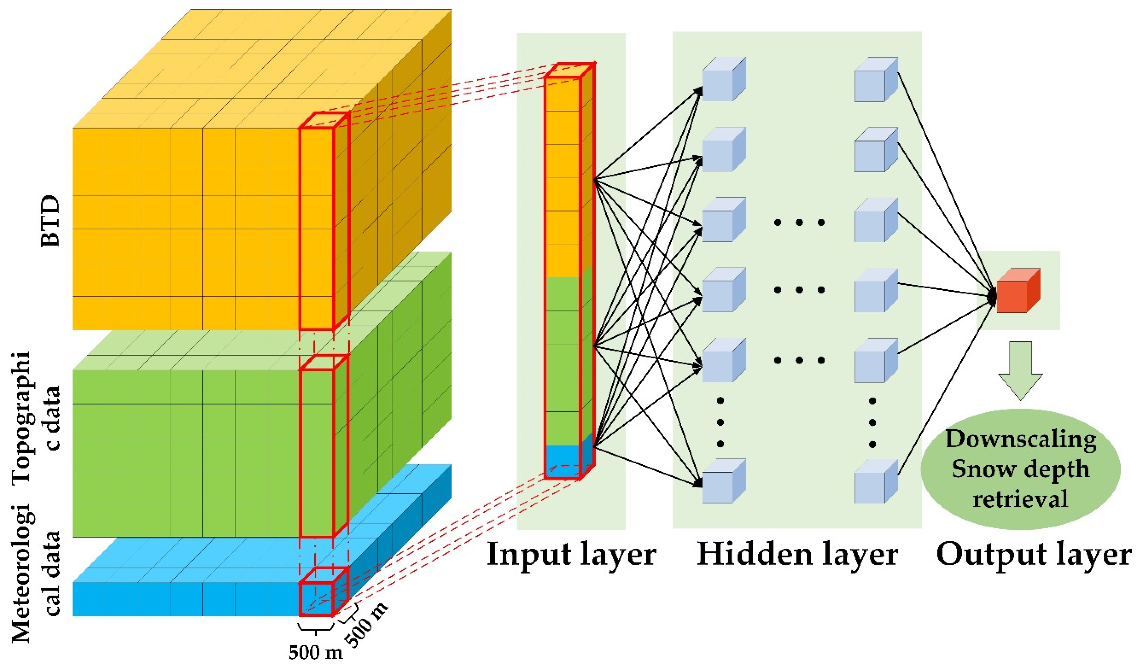
As stated in Section 1, previous studies have focused on the linear relationship between snow depth and microwave BT to retrieve snow depth. However, a nonparametric statistical approach has greater potential to explore the non-linear relationship between snow depth and BTD in a complex ground environment. A neural network, as a classic non-parametric method, has been proved to be effective in the retrieval and estimation of geological parameters. In this study, a three hidden layer backpropagation neural network, with 20, 20 and 10 neurons in the 1st, 2nd and 3rd hidden layer was constructed by the Pytorch framework.

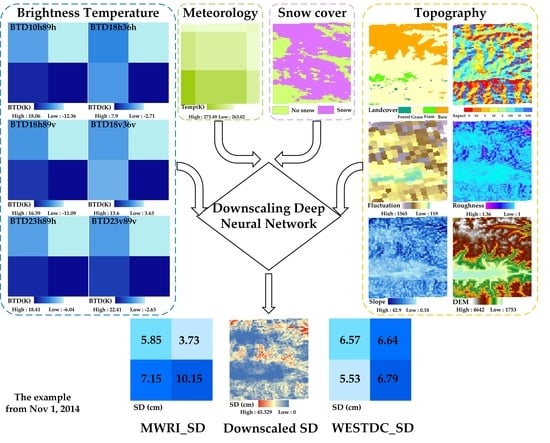
As illustrated in Figure 5, the BTD, topographic data and meteorological data were resampled to the same spatial resolution of 500 m, and then the pixel values of specified longitude and latitude are extracted as input data to match the target task, that is, ground snow depth observation. The computation between neurons in each layer is illustrated in Formula (1):

$$\{\begin{array}{c}{z}^{[l]}=w^{[l]}\times a^{[l-1]}+b^{[l]}\\ a^{[l]}=g(z^{[l]})\end{array}(l=1,2,\cdots ,n)$$

(1)

where is the amount of layers, $l$ represents that the variables belong to the $l\text{-}th$ layer, $w^{[l]}$ is the weight matrix and $b^{[l]}$ is the bias of the layer; is the sigmoid function, a non-linear activation function, is used by the neurons in the third hidden layer, which can capture non-linear relationships between various inputs and snow depth. The backpropagation is a method that repeatedly adjusts weights to minimize the disparity between actual and expected outputs. Mean squared error (MSE) cost function and stochastic gradient descent (SGD) optimization function were used in the proposed deep neural network to minimize a sum of the mean squared error, and SGD is described in Formula (2):

$$\{\begin{array}{c}{w}^{[l]}=w^{[l]}-\alpha \frac{\partial F}{\partial w^{[l]}}\\ b^{[l]}=b^{[l]}-\partial \frac{\partial F}{\partial b^{[l]}}\end{array}(l=1,2,\cdots ,n)$$

(2)

where $F$ is the cost function, $\partial$ is the learning rate, set to 0.001, $w^{[l]}$ and $b^{[l]}$ are the weight matrix and bias vector in the layer $l$.

3.3. Model Evaluation and Accuracy Metrics

The measured snow depth from ground stations was used as the truth value to evaluate the performance of the downscaling model and the accuracy of retrieval results. The specific evaluation criteria included the mean coefficient of determination (R²), root mean squared error (RMSE), positive mean error (PME), negative mean error (NME), average absolute error (MAE) and bias (BIAS). The calculation Formulas (3)–(8) of the five indexes are as follows:

$${\mathrm{R}}^2=1-\frac{{{\displaystyle {\sum }_{i=1}^n(y_i-E(y_i))}}^2}{{{\displaystyle {\sum }_{i=1}^n(E(y_i)-\overline{y})}}^2}$$

(3)

$$\mathrm{RMSE}=\sqrt{\frac{{\displaystyle {\sum }_{i=1}^n{(y_i-E(y_i))}^2}}{n}}$$

(4)

$$\mathrm{MAE}=\frac{1}{n}{\displaystyle {\sum }_{i=1}^n\left|y_i-E(y_i)\right|}$$

(5)

$$\mathrm{PME}=\frac{1}{p}{\displaystyle {\sum }_{i=1}^p(E(y_i)-y_i)},E(y_i)>y_i$$

(6)

$$\mathrm{NME}=\frac{1}{r}{\displaystyle {\sum }_{i=1}^r(E(y_i)-y_i)},E(y_i)<y_i$$

(7)

$$\mathrm{BIAS}=\frac{{\displaystyle {\sum }_{i=1}^n(y_i-E(y_i))}}{n}$$

(8)

In the aforementioned formulas, $y_i$ is the $i\text{-}\mathrm{th}$ measured snow depth from ground station; $E(y_i)$ is the $i\text{-}\mathrm{th}$ retrieved snow depth based on microwave data; $p$ and $r$ are the number of samples whose measured snow depth are greater and less than the retrieved snow depth, respectively; and $n$ is the total number of tested samples.

4. Results

4.1. Corrections of Factors

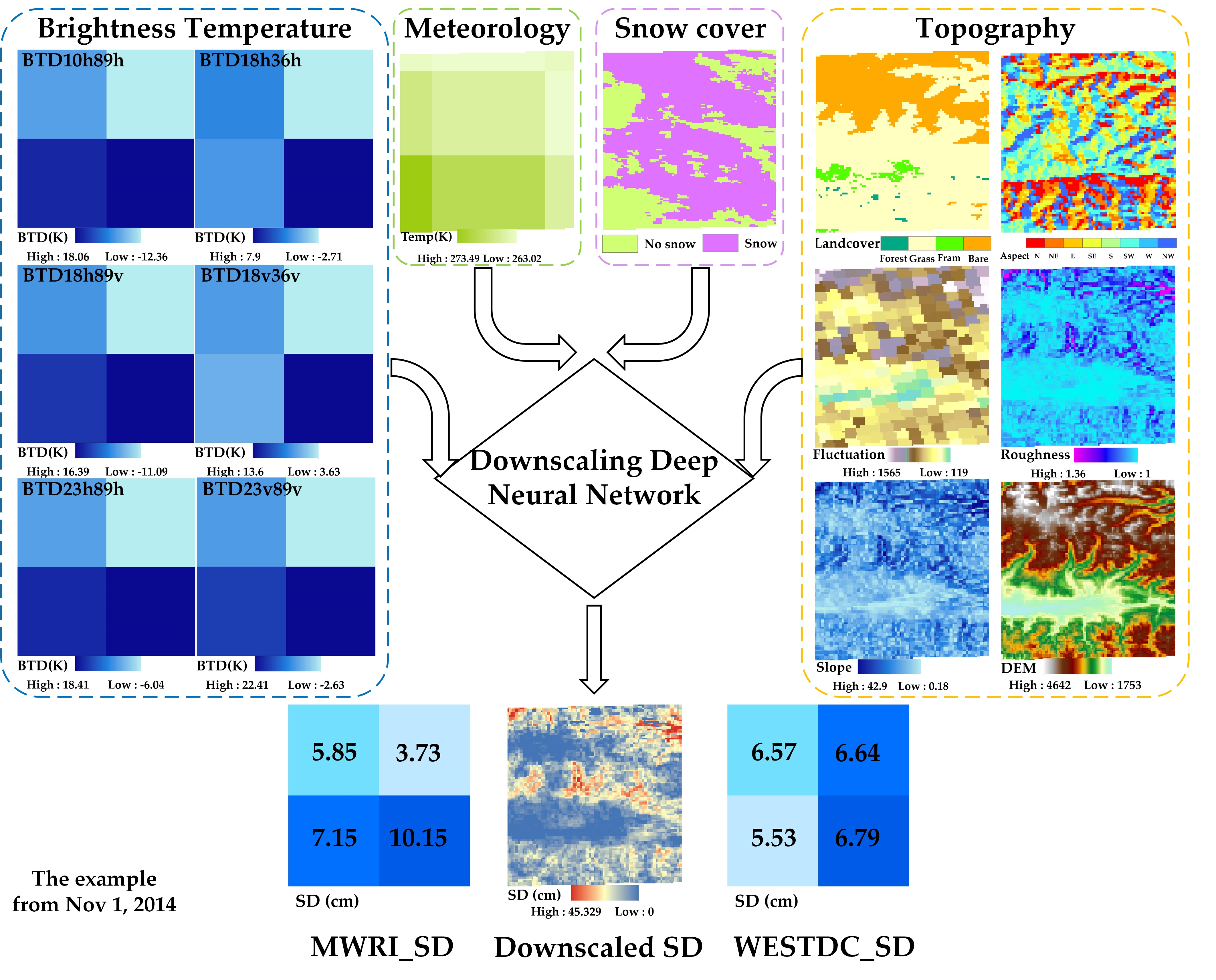
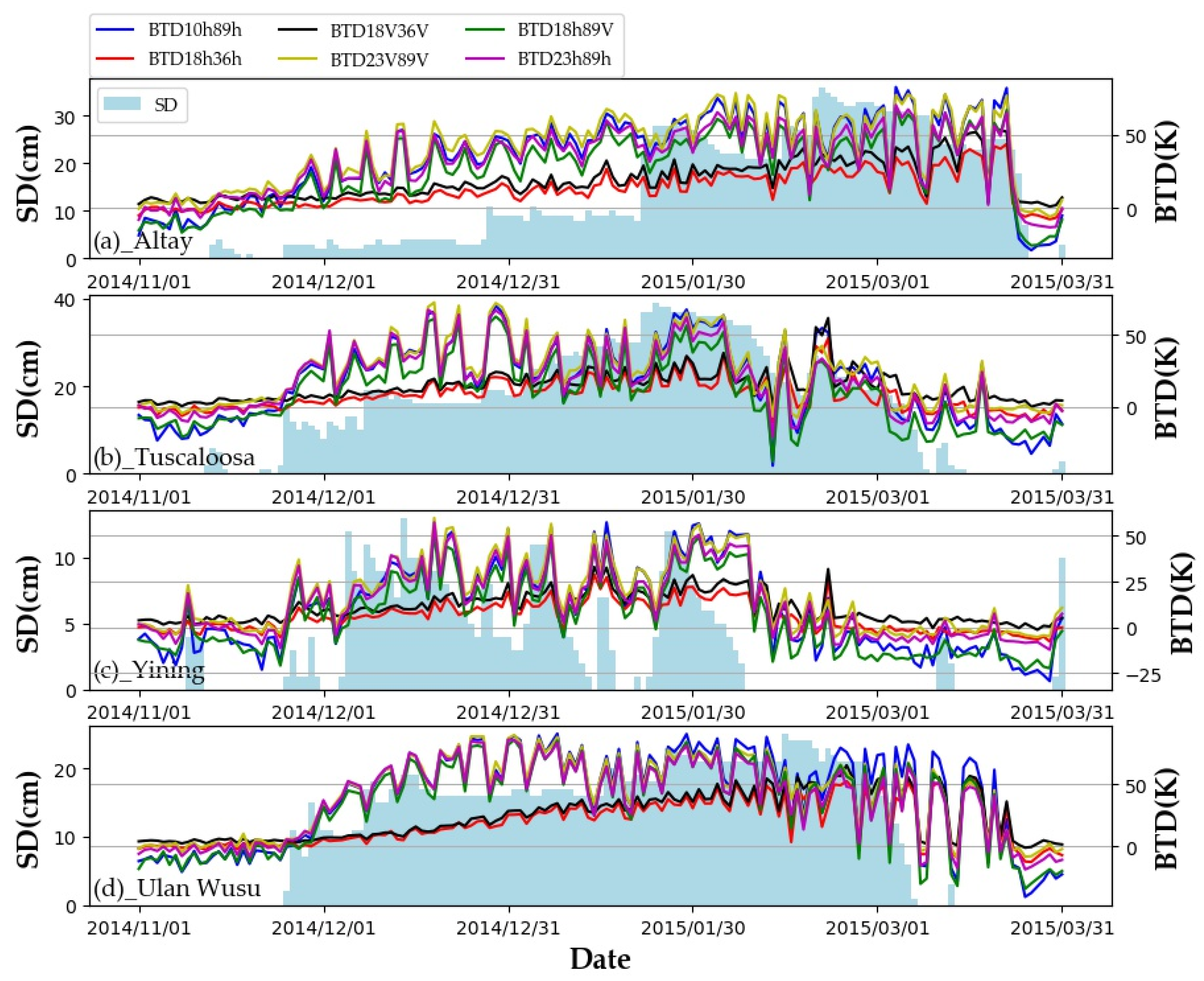
The correlation between snow depth and BTD is described quantitatively in this section. Four typical stations (Altay: 88.08°E, 47.73°N; Tuscaloosa: 83.00°E, 46.73°N; Yining: 81.33°E, 43.95°N; UlanWusu: 85.82°E, 44.28°N) were chosen for factor evaluation. Altay station is located in the covered area of Altai Mountain vein. The mean temperature in cold winter is −23 °C, the mean snow depth in winter is 48 cm, and the annual snow cover days is more than 6 months with a 98.8% coverage rate. In winter, dry snow is dominated and well-distributed in Altay area. The underlying ground is farmland and alpine grassland. Tuscaloosa station is located in Tuscaloosa basin, with cold climate and mean snow depth of 32 cm in winter. As in Altay region, well-distributed dry snow dominates Tuscaloosa basin and the underlying surface is farmland or sparse vegetation, however, the terrain is flatter. The Ili River valley where Yining is located is a bell mouth terrain ringed on three sides by mountains. The water vapor from the Caspian Sea and the Black Sea accumulates here, making the region rich in precipitation and humid climate. The snow with wet feature dominates the hills and mountains, covering the underlying surface of farmland and vegetation heterogeneously. Ulan Wusu station is located in the Economic Zone on the north slope of Tianshan Mountain. The mean snow depth in this area is about 23 cm, and the underlying surface of snow is more complex, including farmland, shrub vegetation and shelterbelt. The above contents are the climate, topography and underlying surface characteristics of four typical stations in NX.

Four representative regions were selected to assess the correlation between BTD and snow depth. The BT polarization difference in Altay, Tuscaloosa, Yining and Ulan Wusu from 1 November 2014 to 31 March 2015, as well as the snow depth and ground surface temperature recorded by meteorological stations on the corresponding date. It can be seen that there are obvious changes in the polarization difference of MWRI BT corresponding to the snow cover, especially the brightness temperature difference between the low-frequency channel and the high-frequency channel (Figure 6). The specific features are as follows: (1) BTD18h36h and BTD18v36v increased with the accumulation of new snow and the increase of snow depth; (2) BTD decreases with the increase of the ground surface temperature, even the result is negative. Therefore, the air temperature factor should be considered in the passive microwave snow depth retrieval model.

Detailed coefficient of determination between snow depth and BTD at four typical stations were described in

Table 2. Coefficient of determination between snow depth and BTD at Altay, Tuscaloosa, Yining and Ulan Wusu.

BTD	Altay_R2	Tuscaloosa_R2	Yining_R2	Ulan Wusu_R2	Mean_R2
BTD10h89h	0.4391	0.5258	0.4025	0.5342	0.4753
BTD18h36h	0.6037	0.5286	0.2261	0.2958	0.4136
BTD18v36v	0.6243	0.4763	0.1872	0.2902	0.3945
BTD23v89v	0.4061	0.4546	0.3882	0.5709	0.4550
BTD18h89v	0.4305	0.4014	0.4024	0.5331	0.4419
BTD23h89h	0.3876	0.4208	0.4045	0.5445	0.4394
Mean_R2	0.4819	0.4679	0.3352	0.4615	0.4366

. Generally speaking, except for the BTD18h36h and BTD18v36v data of Yining station, the other BTD data have a high coefficient of determination with snow depth. Altay, where dry snow is evenly distributed, is the best place for satellite synchronous observation and ground verification in snow remote-sensing research. The coefficient of determination between BTD and snow depth shows the best result and reaches 0.4819. Moreover, the coefficient of determination between BTD18h36h, BTD18v36v and snow depth, which is widely used in the classical Chang algorithm, is as high as 0.6037 and 0.6243. The coefficient of determination at Yining station is relatively poor, which is related to the humid climate in the valley and the characteristic of wet snow. Only from the perspective of BTD, the mean R² of the six BTDs and snow depth at each station are relatively close, except that the poor coefficient of determination of BTD18v36v in Yining station reduces the mean value. Therefore, the six BTDs can be used to retrieve the snow depth in NX based on the contents described in the above figures and table.

The radiation BT of snow cover in the high-frequency channel decrease obviously. Thus, the BTD between high and low frequency channels is used as scattering index, its change and threshold value are used as a characteristic index in retrieval algorithm. In the actual snow depth microwave radiation modeling, the influence of surface roughness (high mountain, hilly, flat, etc.) and land cover parameters (glacier, vegetation, forest, desert, desert, etc.) should be considered. Moreover, microwave radiation can penetrate snow and detect radiation from the underlying surface, which indicates that the detection results are affected by the volume scattering caused by the difference of soil physical properties in vertical direction. Therefore, the natural environmental differences of snowfields must be considered comprehensively in snow depth retrieval.

4.2. Case Study of Spatial Distribution

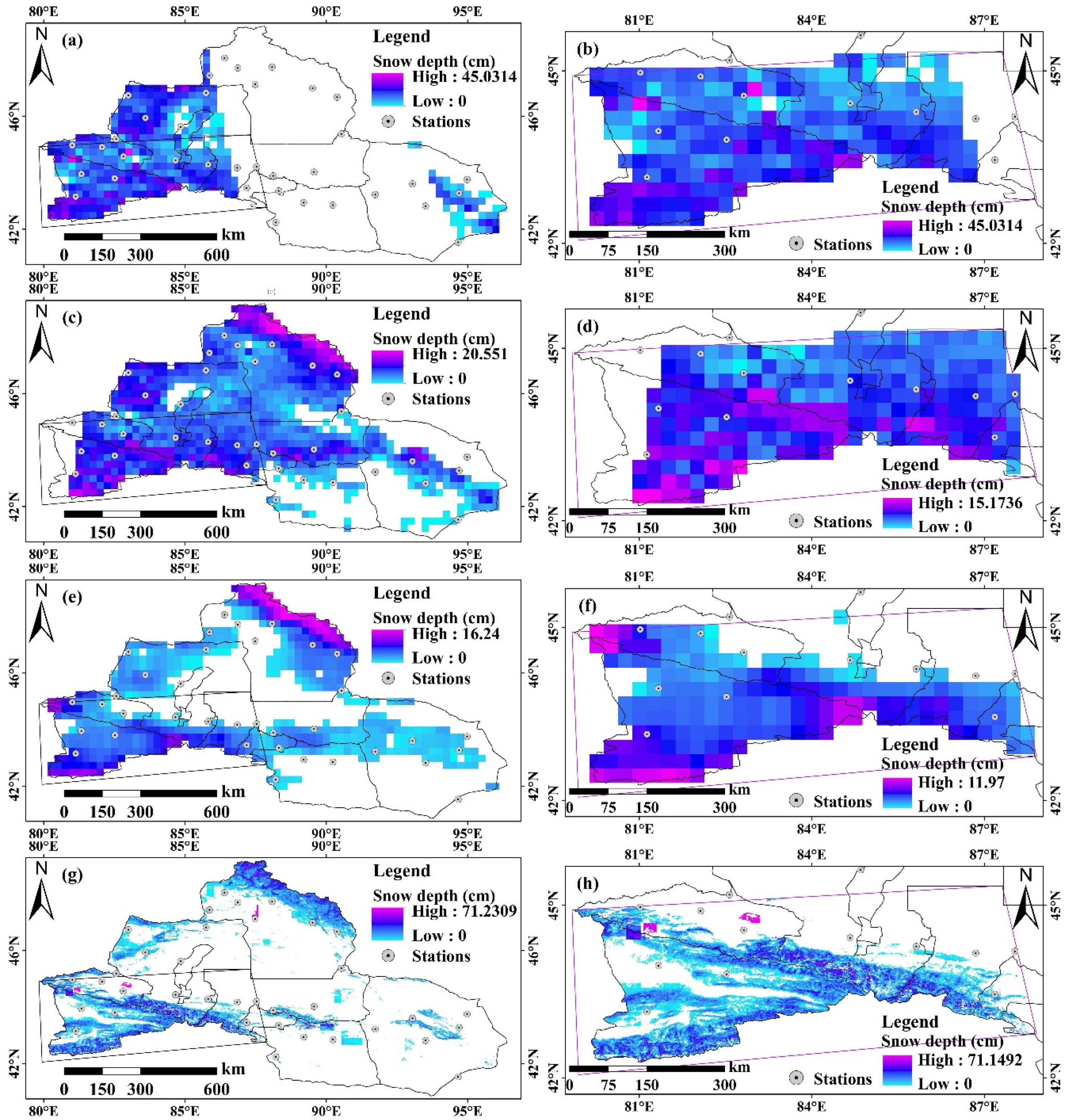
The comparison of snow depth mapping was used to show the consistency of the spatial distribution among the downscaled snow depth and existing snow depth datasets, and try to present more detailed information, especially in alpine regions and river valleys. The snow depth mapping for 1 December 2014, as a typical example, is shown in Figure 7.

The downscaling snow depth map (Figure 7g), the corresponding WESTDC snow depth datasets (Figure 7e), and the official ascending (Figure 7a) and descending (Figure 7c) snow depth datasets via Jiang’s [63] algorithm for the same day are shown. Due to orbital scanning, both official ascending and descending snow depth maps have large strip gaps across NX. Data only based on a single orbit will lead to missing snow depth information. WESTDC snow depth map reflects the snow distribution covering the entire NX (Figure 7e). However, the proposed downscaling approach can derive snowpack information and provide details on snow depth variations at 500 m spatial resolution. As shown in Figure 7, on 1 December 2014, the snow cover was primarily distributed in Altai Mountains, Tianshan Mountains and Western Tianshan Mountains. There is also a few shallow snow distributed over Hami area in the eastern of NX and Tuscaloosa in the western of NX. Tianshan Mountains and the Altay area are the two high-value regions of snow depth and Tianshan Mountains were selected for detailed display. In Figure 7h enlarged views, the snow depth distribution varies with the altitude of the mountains, showing obvious texture characteristics, that are consistent with the actual situation. WESTDC snow depth datasets, official ascending and descending snow depth datasets also described the regional snow depth information with coarse resolution, especially WESTDC snow depth datasets has good consistency with the snow depth map generated by the downscaling approach in spatial distribution. However, extensive heterogeneity of snow depth is only shown in the downscaled snow depth mapping.

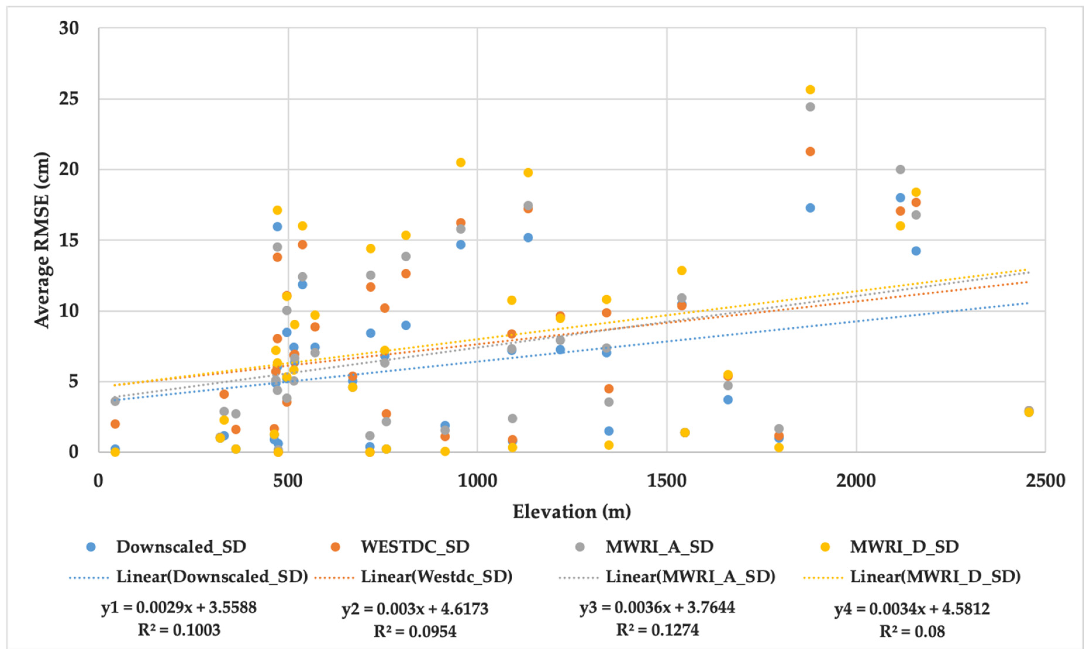
4.3. Accuracy Validation

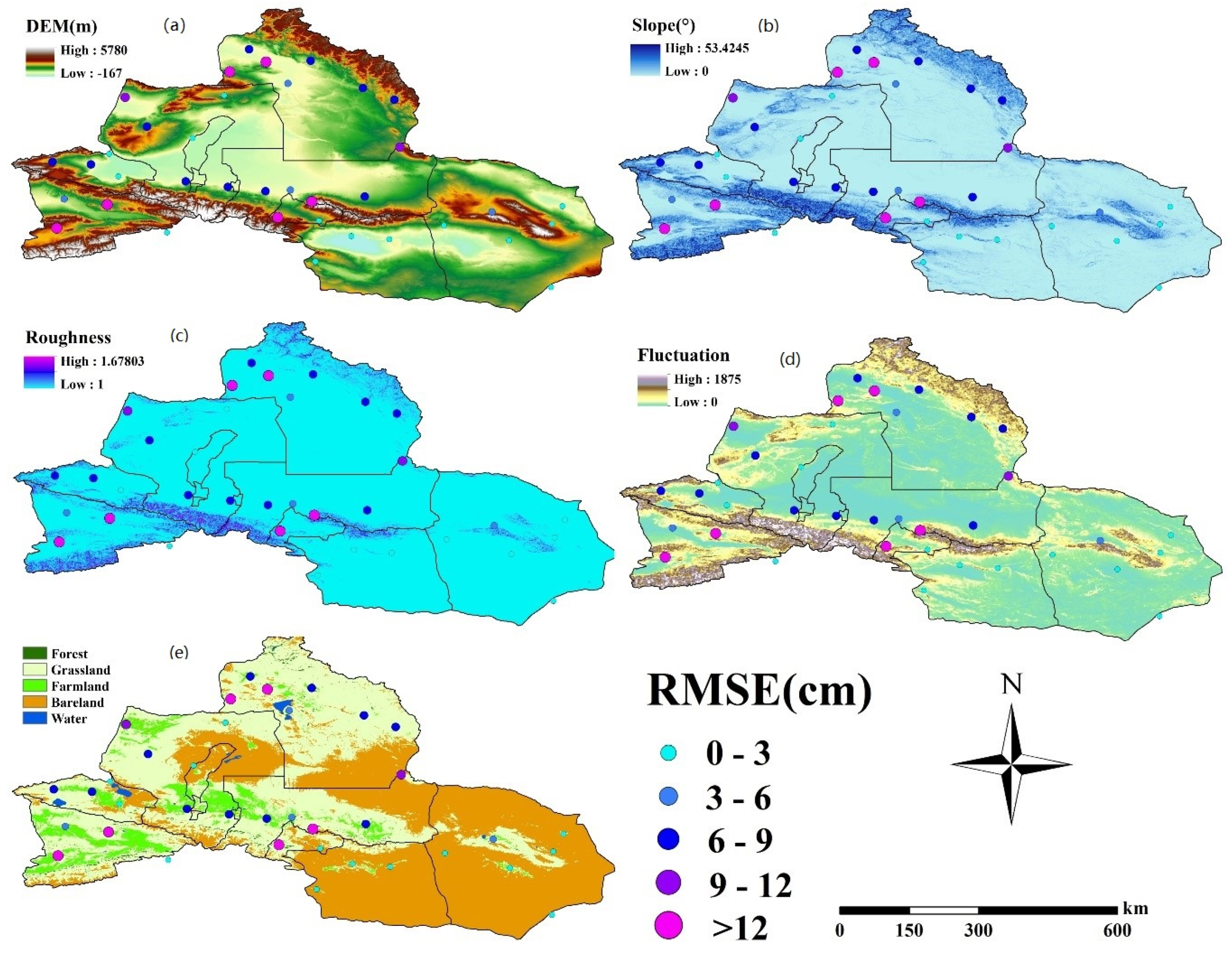
Snow depth observations from 37 national meteorological stations in NX (from 1 November 2014 to 31 March 2015) were selected to validate and evaluate the accuracy of downscaled snow depth and to compare the accuracy of MWRI_A, MWRI_D, WESTDC_SD. The detailed RMSE, PME, NME, MAE and BIAS are described in

Table 3. The root mean square error (RMSE), positive mean error (PME), negative mean error (NME), average absolute error (MAE) and bias (BIAS) for four types of snow depth (SD) dataset for NX base ground stations.

Snow Depth Datasets	RMSE (cm)	PME (cm)	NME (cm)	MAE (cm)	BIAS (cm)
Downscaled SD	8.16	3.78	−8.49	4.73	−2.71
WESTDC_SD	9.38	2.95	−10.06	5.36	−2.78
MWRI_A_SD	9.45	4.42	−10.11	5.49	−3.73
MWRI_D_SD	10.55	3.03	−11.16	6.13	−6.28

. MWRI_D_SD shows the highest RMSE of 10.55 cm, highest NME of −11.16 cm, highest MAE of 6.13 cm, and highest BIAS of −6.28 cm, followed by MWRI_A_SD with an RMSE of 9.45 cm, PME of 4.42 cm, NME of −10.11 cm, MAE of 5.49 cm and BIAS of −3.73 cm. WESTDC_SD, a widely reported and approved snow depth dataset [2,15,62], is more accurate than MWRI_A_SD and MWRI_D_SD in NX, with the lowest PME of 2.95 cm. PME values are lower than NME of all SD datasets. There are significant errors of the snow depth retrieved by microwave data compared with ground observations in NX, but the difference between PME and NME for downscaled SD is minimal. Most importantly, the downscaled snow depth has the best accuracy compared to the other three snow depth datasets, with the lowest RMSE of 8.16 cm, MAE of 4.73 cm and BIAS of −2.71 cm.

In the overall accuracy evaluation, downscaled snow depth is dominant compared to snow depth datasets, while detailed results based on snow comparison at different depths are described in

Table 4. RMSE of four types of snow depth datasets for NX under different value levels.

SD (cm)	Downscaled SD	WESTDC_SD	MWRI_A_SD	MWRI_D_SD
0 ≤ SD ≤ 3 cm	1.03	3.60	2.49	4.06
3 < SD ≤ 6 cm	4.49	5.41	3.92	5.41
6 < SD ≤ 10 cm	6.30	5.77	8.13	6.73
10 < SD ≤ 30 cm	11.15	13.11	15.77	13.11
SD > 30cm	20.88	26.40	27.85	24.09

. Similar to the results in Table 3, downscaled snow depth performs best at different snow depth levels, followed by WESTDC_SD and MWRI_A_SD, and MWRI_D_SD has the poorest accuracy performance.

5. Discussion

5.1. Improvement of Snow Cover

The daily snow cover used for snow depth retrieval in this study is combined from the collaborative retrieval of MODIS optical data and MWRI microwave data in different time phases in a single day. The variation of snow cover proportion of various snow datasets from 1 November 2014 to 31 March 2015 is described in Figure 8. In particular, MXD10A1 is the result of cloud removal synthesized by MOD10A1 and MYD10A1. MWRI_snowcover is the snow cover information retrieved from MWRI data by the decision tree algorithm. Composite snowcover is the final snow cover result synthesized by MXD10A1 and MWRI_snowcover. In a snow season, the mean snow cover percentage of MOD10A1 is 19.01%, with the highest value 50.02% and the lowest value 0.16%. In contrast, MYD10A1 is a snow dataset of satellite transit in the afternoon. The enhancement of solar radiation promotes the water vapor to rise and eventually leads to the increase of clouds. Therefore, MYD10A1 has more cloud proportion and less snow proportion, with a mean value of 18.00%, the highest value of 49.85% and lowest value of 0.09%. Due to the small variation of snow cover and the great change of cloud movement, the maximum snow cover MXD10A1 based on optical data can be obtained by the intersection of cloud pixels of MOD10A1 and MYD10A1, with a mean ratio of 25.61%.

However, it is still impossible to detect the snow pixels under the clouds. Microwave radiation data was able to penetrate the clouds and detect the land cover. Thus, the results retrieved by optical data were accepted for cloud-free area, while the results retrieved by microwave data were accepted for cloud-covered area. From 1 November 2014 to 31 March 2015, the mean snow cover ratio of the region increased to 54.59% after the collaborative observation of the two types of data.

5.2. A Rough Comparison of Snow Storage at the Study Area

The snow storage in pixel scale is calculated by units of the pixels, which is the total volume of snow in a specific area. The general Equation (9) is given as follows:

$$v_{snow}={\displaystyle \sum _{i=1}^N{A}_i\times S{D}_i}$$

(9)

where $A$ is the snow area and $SD$ is snow depth at pixel scale, $v_{snow}$ is the snow storage. The quantitative calculation of snow storage in the study area is of great significance to the monitoring and development of snow solid water resources. More intuitively, it can provide a way for the comparison and verification of snow depth datasets with different scales.

Figure 9 illustrates the same change trend of snow storage generated from three snow depth datasets in NX from 1 November 2014 to 31 March 2015. The snow storage increased from the beginning of November to the peak in February of the next year and then decreased from the latter part of February. From 1 November to Mid-December, MWRI_SD has the largest snow storage, WESTDC has the least snow storage, downscaled snow depth ranked second. The snow storage and rising trends of downscaled snow depth and WESTDC have good consistency from mid-December to latter January of the next year. Starting from the snowmelt phase in February, the downscaled snow depth has the fastest decreasing trend. It is worth noting that during the snowmelt stage, both downscaled snow depth and MWRI_SD fluctuate and oscillate, while the downward trend of WESTDC is relatively flat. First of all, this difference may be due to the lower spatial resolution and sensitivity of MWRI than that of SSMI/S, and the relatively poor accuracy of BT. Secondly, downscaled snow depth and MWRI_SD have the same trend of fluctuation in the same period, but the amplitude of downscaled snow depth fluctuation is smaller, which indicates the results of downscaled snow depth show better stability than MWRI_SD. Finally, with the increase of temperature in March, accelerated snow melting leads to an increase in liquid water and a greater proportion of wet snow. In the above study, wet snow pixels are eliminated in the snow recognition based on decision tree algorithm. Therefore, since the snowmelt period in March, the snow storage calculated based on the downscaling algorithm is the smallest compared with the other two snow data.

5.3. Error Analysis Based on Multiple Factors

In Section 4.3, the accuracy of downscaled snow depth has been validated and evaluated, which shows good performance compared with the snow depth datasets with 25 km resolution. In this section, we will analyze the error distribution under various terrain conditions, and discuss the influence of terrain factors on the error of snow depth retrieval. Figure 10 reveals that average RMSE of each station (from 1 November 2014 to 31 March 2015) has a large difference. However, the spatially consistent trends in error are consistent across the four snow depth datasets. The blue points represent the average RMSE in the downscaled snow depth datasets, which is the lowest of the four SD datasets. This is consistent with the findings in Section 4.3. The three sites with the highest RMSE are Nilke station (82.52°E, 43.80°N), Shao su station (81.13°E, 43.15°N) and Tianchi station (88.12°E, 43.88°N). With the exception of Tianchi station, which is located in Tianchi Scenic Area near Urumqi, the other two stations are located in Ili River Valley. As mentioned in Section 4.1, the unstable snow characteristics in the Ili River valley, which is dominated by wet snow, create significant uncertainty in snow depth retrieval and hence high errors. Another interesting finding is that the mean RMSE is positively correlated with elevation, which indicates that the accuracy of snow depth retrieval decreases with elevation. By comparing the blue line (Downscaled_SD), orange line (Westdc_SD), gray line (MWRI_A_SD) and yellow line (MWRI_D_SD), we can find that the slope of the blue line is the smallest, which also shows that RMSE of downscaled snow depth increases the slowest with the increase of elevation, showing the best performance.

The spatial distribution of RMSE of downscaled snow depth in NX for different DEM (Figure 11a), Slope (Figure 11b), Roughness (Figure 11c), Fluctuation (Figure 11d) and Land cover (Figure 11e) were described in Figure 11. High RMSE value stations are found in the Tianshan Mountains, Western Tianshan Mountains and Altai Mountains. An intriguing result is that stations of high RMSE value are surrounded by mountains on both sides. The two stations located in the northwest of the northern border are surrounded by the Altai Mountains and small hills. Two high-value stations in the Ili river valley are also wrapped by Jengish Chokusu and the Central Tianshan Mountains, while another two stations are surrounded by the Central Tianshan Mountains and Mount Bogda. Generally speaking, the high-value stations of RMSE are primarily distributed in mountain areas with complex terrain. The surface slope is steep, the values of roughness and fluctuation are large, and the characteristics of snow cover are unstable, while the low-value stations of RMSE are mostly distributed in the areas with gentle terrain. This also illustrates the interference of complex terrain to snow depth detection.

We also counted the distribution of RMSE across different aspects. As shown in Figure 12, the values of RMSE are larger in the west and south and east directions and smaller in the remaining directions. This may be related to the insolation conditions, where the west, south, and east sides receive more solar radiation during the day, which changes the moisture, density, snow particle size, and other minor parameters of the snowpack, resulting in a decrease in the accuracy of the snow depth retrieval.

5.4. Advantages and Limitations

Downscaling a snow depth model based on deep learning has the two advantages. Firstly, based on the validation of snow depth data measured by ground observation stations, the proposed model shows the best accuracy and minimum error compared with the widely reported public datasets. Secondly, all the input variables can be obtained quickly, which is helpful for the future business promotion of the model.

Although the downscaling snow depth model performs well in accuracy and spatial resolution, there are still some limitations that warrant further improvement. We compared the altitude distribution of observation stations with that of the whole NX. There is a large elevation difference in NX, from basin to hill to mountain. As shown in

Table 5. Stations distribution and NX across elevation.

Elevation Range	NX across Elevation	Stations Distribution across Elevation
<500 m	18.47%	29.73%
500 m–1000 m	31.95%	32.43%
1000 m–1500 m	22.79%	16.22%
1500 m–2000 m	10.99%	13.51%
>2000 m	15.81%	8.11%

, the proportion elevation ranges from 500 m to 1000 m, from 1000 m to 1500 m in NX it is 31.95% and 22.79%, respectively. The location of 36 observation stations in NX was more determined by traffic, terrain, population and other factors. Therefore, the proportion of observation stations below 500 m, from 500 m to 1000 m reaches 29.73% and 32.43%. Nevertheless, as shown in Figure 13, Stations distribution across elevation is similar to NX across elevation. Therefore, the upscaling performance of the algorithm is credible.

Similar to the above study, stations distribution and NX across aspects were compared in

Table 6. Stations distribution and NX across aspect.

Aspect	NX across Aspect	Stations Distribution across Aspect
North	17.32%	27.03%
Northeast	14.85%	5.41%
East	8.02%	8.11%
Southeast	8.81%	13.51%
South	14.03%	24.32%
Southwest	14.35%	5.41%
West	10.20%	5.41%
Northwest	12.43%	10.81%

and Figure 14. The distribution of aspects in the whole NX is relatively balanced, with the most pixels in the north aspect, accounting for 17.32% of all pixels, and the least pixels in the east aspect, accounting for 8.02%. Stations’ distribution across aspect is quite different, with the highest proportion of 27.03% in north aspect and lowest proportion of 5.41% in northeast aspect, southwest aspect and west aspect. As shown in Figure 14, the aspect distribution of the stations is different from that of the whole NX, and the algorithm has limitations in the scalability of the aspect.

Due to the safety of the staff and the convenience of material transportation, the ground meteorological observation stations are usually located in the flat and small slope area. Therefore, it is difficult to discuss the scalability of the algorithm on the slope. Based on the above analysis, there are many limitations on the scalability of the downscaling snow depth model in different altitudes, aspect, slope and other environments.

6. Conclusions

Accurate high spatial resolution snow depth mapping is of great importance for regional snow disaster assessment and hydrological simulation, especially for NX with a complex topography and abundant snow. Microwave data with coarse spatial resolution are not enough to detect the spatiotemporal heterogeneity of snow depth. This manuscript proposes a deep learning approach for spatial downscaling of snow depth over the alpine region. Compared to the traditional remote-sensing snow depth retrieval method based on linear regression, this method can better adapt to arid and semi-arid regions with complex topographical and specific geo-meteorological features. Accuracy of downscaled snow depth estimations has been improved compared to existing snow datasets, with the lowest RMSE and MAE (8.16 cm and 4.73 cm, respectively) compared with WESTDC_SD (9.38 cm and 5.36 cm), MWRI_A_SD (9.45 cm and 5.49 cm) and MWRI_D_SD (10.55 cm and 6.13 cm). Furthermore, the downscaled snow depth depicts the distribution characteristics of snow depth along with the altitude in the alpine region. The above results are enough to prove the effeteness and superiority of this method. Although the method has multi-element requirements for the input data and has a limitation on retrieval scene, it has achieved fruitful results in the downscaling snow depth retrieval, which also provides a reference for subsequent snow depth retrieval.

References

1. Lievens, H.; Demuzere, M.; Marshall, H.-P.; Reichle, R.H.; Brucker, L.; Brangers, I.; De Rosnay, P.; Dumont, M.; Girotto, M.; Immerzeel, W.W.; et al. Snow depth variability in the Northern Hemisphere mountains observed from space. Nat. Commun. 2019, 10, 1–12. [Google Scholar] [CrossRef] [PubMed]
2. Che, T.; Li, X.; Jin, R.; Armstrong, R.; Zhang, T. Snow depth derived from passive microwave remote-sensing data in China. Ann. Glaciol. 2008, 49, 145–154. [Google Scholar] [CrossRef] [Green Version]
3. Rittger, K.; Painter, T.H.; Dozier, J. Assessment of methods for mapping snow cover from MODIS. Adv. Water Resour. 2013, 51, 367–380. [Google Scholar] [CrossRef]
4. Masson, T.; Dumont, M.; Mura, M.D.; Sirguey, P.; Gascoin, S.; Dedieu, J.-P.; Chanussot, J. An assessment of existing method-ologies to retrieve snow cover fraction from MODIS data. Remote Sens. 2018, 10, 619. [Google Scholar] [CrossRef] [Green Version]
5. Gao, J.; Huang, X.; Ma, X.; Feng, Q.; Liang, T.; Xie, H. Snow disaster early warning in pastoral areas of Qinghai Province, China. Remote Sens. 2017, 9, 475. [Google Scholar] [CrossRef] [Green Version]
6. Dozier, J. Spectral signature of alpine snow cover from the landsat thematic mapper. Remote Sens. Environ. 1989, 28, 9–22. [Google Scholar] [CrossRef]
7. Deronde, B.; Debruyn, W.; Gontier, E.; Goor, E.; Jacobs, T.; Verbeiren, S.; Vereecken, J. 15 years of processing and dissemination of SPOT-VEGETATION products. Int. J. Remote Sens. 2014, 35, 2402–2420. [Google Scholar] [CrossRef]
8. Harrison, A.R.; Lucas, R. Multi-spectral classification of snow using NOAA AVHRR imagery. Int. J. Remote Sens. 1989, 10, 907–916. [Google Scholar] [CrossRef]
9. Salomonson, V.; Appel, I. Estimating fractional snow cover from MODIS using the normalized difference snow index. Remote Sens. Environ. 2004, 89, 351–360. [Google Scholar] [CrossRef]
10. Painter, T.H.; Rittger, K.; McKenzie, C.; Slaughter, P.; Davis, R.E.; Dozier, J. Retrieval of subpixel snow covered area, grain size, and albedo from MODIS. Remote Sens. Environ. 2009, 113, 868–879. [Google Scholar] [CrossRef] [Green Version]
11. Notarnicola, C.; Duguay, M.; Mölg, N.; Schellenberger, T.; Tetzlaff, A.; Monsorno, R.; Costa, A.; Steurer, C.; Zebisch, M. Snow cover maps from MODIS images at 250 m resolution, part 1: Algorithm description. Remote Sens. 2013, 5, 110–126. [Google Scholar] [CrossRef] [Green Version]
12. Notarnicola, C.; Duguay, M.; Mölg, N.; Schellenberger, T.; Tetzlaff, A.; Monsorno, R.; Costa, A.; Steurer, C.; Zebisch, M. Snow cover maps from MODIS images at 250 m resolution, part 2: Validation. Remote Sens. 2013, 5, 1568–1587. [Google Scholar] [CrossRef] [Green Version]
13. Di Marco, N.; Righetti, M.; Avesani, D.; Zaramella, M.; Notarnicola, C.; Borga, M. Comparison of MODIS and model-derived snow-covered areas: Impact of land use and solar illumination conditions. Geosciences 2020, 10, 134. [Google Scholar] [CrossRef] [Green Version]
14. Yang, J.; Jiang, L.; Dai, L.; Pan, J.; Wu, S.; Wang, G. The consistency of SSM/I vs. SSMIS and the influence on snow cover detection and snow depth estimation over China. Remote Sens. 2019, 11, 1879. [Google Scholar] [CrossRef] [Green Version]
15. Dai, L.; Che, T.; Ding, Y.; Hao, X. Evaluation of snow cover and snow depth on the Qinghai–Tibetan Plateau derived from passive microwave remote sensing. Cryosphere 2017, 11, 1933–1948. [Google Scholar] [CrossRef] [Green Version]
16. Chang, A.T.C.; Foster, J.L.; Hall, D.K. Nimbus-7 SMMR derived global snow cover parameters. Ann. Glaciol. 1987, 9, 39–44. [Google Scholar] [CrossRef] [Green Version]
17. Aschbacher, J. Land Surface Studies and Atmospheric Effects by Satellite Microwave Radiometry. Ph.D. Thesis, University of Innsbruck, Innsbruck, Austria, 1989. [Google Scholar]
18. Che, T. Study on Passive Microwave Remote Sensing of Snow and Snow Data Assimilation Method. Ph.D. Thesis, Chinese Academy of Sciences, Lanzhou, China, 2006. [Google Scholar]
19. Foster, J.L.; Sun, C.; Walker, J.P.; Kelly, R.; Chang, A.; Dong, J.; Powell, H. Quantifying the uncertainty in passive microwave snow water equivalent observations. Remote Sens. Environ. 2005, 94, 187–203. [Google Scholar] [CrossRef]
20. Tedesco, M.; Narvekar, P.S. Assessment of the NASA AMSR-E SWE product. IEEE J. Sel. Top. Appl. Earth Obs. Remote Sens. 2010, 3, 141–159. [Google Scholar] [CrossRef]
21. Josberger, E.G.; Mognard, N.M. A passive microwave snow depth algorithm with a proxy for snow metamorphism. Hydrol. Process. 2002, 16, 1557–1568. [Google Scholar] [CrossRef]
22. Kelly, R.; Chang, A.; Tsang, L.; Foster, J.L. A prototype AMSR-E global snow area and snow depth algorithm. IEEE Trans. Geosci. Remote Sens. 2003, 41, 230–242. [Google Scholar] [CrossRef] [Green Version]
23. Pulliainen, J.T.; Grandell, J.; Hallikainen, M.T. HUT snow emission model and its applicability to snow water equivalent retrieval. IEEE Trans. Geosci. Remote Sens. 1999, 37, 1378–1390. [Google Scholar] [CrossRef]
24. Chen, C.-T.; Nijssen, B.; Guo, J.; Tsang, L.; Wood, A.; Hwang, J.-N.; Lettenmaier, D. Passive microwave remote sensing of snow constrained by hydrological simulations. IEEE Trans. Geosci. Remote Sens. 2001, 39, 1744–1756. [Google Scholar] [CrossRef]
25. Hung, C.W.; Mao, W.L.; Huang, H.Y. Modified PSO algorithm on recurrent fuzzy neural network for system identification. Intell. Autom. Soft Comput. 2019, 25, 329–341. [Google Scholar]
26. Xu, F.; Zhang, X.F.; Xin, Z.H.; Yang, A. Investigation on the Chinese text sentiment analysis based on convolutional neural networks in deep learning. Comput. Mater. Contin. 2019, 58, 697–709. [Google Scholar] [CrossRef] [Green Version]
27. Guo, Y.C.; Li, C.; Liu, Q. R2N: A novel deep learning architecture for rain removal from single image. Comput. Mater. Contin. 2019, 58, 829–843. [Google Scholar] [CrossRef] [Green Version]
28. Wu, H.; Liu, Q.; Liu, X. A review on deep learning approaches to image classification and object segmentation. Comput. Mater. Contin. 2019, 60, 575–597. [Google Scholar] [CrossRef] [Green Version]
29. Zhang, X.; Lu, W.; Li, F.; Peng, X.; Zhang, R. Deep feature fusion model for sentence semantic matching. Comput. Mater. Contin. 2019, 61, 601–616. [Google Scholar] [CrossRef]
30. Senthilnath, J.; Varia, N.; Dokania, A.; Anand, G.; Benediktsson, J.A. Deep TEC: Deep transfer learning with ensemble classifier for road extraction from UAV imagery. Remote Sens. 2020, 12, 245. [Google Scholar] [CrossRef] [Green Version]
31. Xu, Y.; Xie, Z.; Feng, Y.; Chen, Z. Road Extraction from high-resolution remote sensing imagery using deep learning. Remote Sens. 2018, 10, 1461. [Google Scholar] [CrossRef] [Green Version]
32. Wang, Y.B.; Long, M.S.; Wang, J.M.; Gao, Z.F.; Yu, P.S. PredRNN: Recurrent neural networks for predictive learning using spatiotemporal LSTMs. In Proceedings of the 31st Conference on Neural Information Processing Systems (NIPS 2017), Long Beach, CA, USA, 4–9 December 2017. [Google Scholar]
33. Chen, X.; Xu, C.; Yang, X.; Tao, D. Long-term video prediction via criticization and retrospection. IEEE Trans. Image Process. 2020, 29, 7090–7103. [Google Scholar] [CrossRef]
34. Xue, Y.; Forman, B.A. Comparison of passive microwave brightness temperature prediction sensitivities over snow-covered land in North America using machine learning algorithms and the Advanced Microwave Scanning Radiometer. Remote Sens. Environ. 2015, 170, 153–165. [Google Scholar] [CrossRef]
35. De Gregorio, L.; Callegari, M.; Marin, C.; Zebisch, M.; Bruzzone, L.; Demir, B.; Strasser, U.; Marke, T.; Günther, D.; Nadalet, R.; et al. A novel data fusion technique for snow cover retrieval. IEEE J. Sel. Top. Appl. Earth Obs. Remote Sens. 2019, 12, 2862–2877. [Google Scholar] [CrossRef] [Green Version]
36. Ahmad, J.A.; Forman, B.A.; Kwon, Y.H. Analyzing machine learning predictions of passive microwave brightness temperature spectral difference over snow-covered terrain in High Mountain Asia. Front. Earth Sci. 2019, 7, 1–15. [Google Scholar] [CrossRef] [Green Version]
37. Tedesco, M.; Pulliainen, J.; Takala, M.; Hallikainen, M.; Pampaloni, P. Artificial neural network-based techniques for the retrieval of SWE and snow depth from SSM/I data. Remote Sens. Environ. 2004, 90, 76–85. [Google Scholar] [CrossRef]
38. Tabari, H.; Marofi, S.; Abyaneh, H.Z.; Sharifi, M.R. Comparison of artificial neural network and combined models in estimating spatial distribution of snow depth and snow water equivalent in Samsami basin of Iran. Neural Comput. Appl. 2009, 19, 625–635. [Google Scholar] [CrossRef]
39. Xiao, X.; Zhang, T.; Zhong, X.; Shao, W.; Li, X. Support vector regression snow-depth retrieval algorithm using passive microwave remote sensing data. Remote Sens. Environ. 2018, 210, 48–64. [Google Scholar] [CrossRef]
40. Liu, J.; Zhang, Y.; Cheng, X.; Hu, Y. Retrieval of snow depth over arctic sea ice using a deep neural network. Remote Sens. 2019, 11, 2864. [Google Scholar] [CrossRef] [Green Version]
41. Liang, J.; Liu, X.; Huang, K.; Li, X.; Shi, X.; Yaning, C.; Li, J. Improved snow depth retrieval by integrating microwave brightness temperature and visible/infrared reflectance. Remote Sens. Environ. 2015, 156, 500–509. [Google Scholar] [CrossRef]
42. Sun, Z.W.; Yu, P.S.; Xia, L.; Wu, S.L.; Jiang, L.M.; Guo, L. Progress in study of snow parameter inversion by passive microwave remote sensing. Remote Sens. Land Resour. 2015, 27, 9–15. (In Chinese) [Google Scholar]
43. Wang, Y.L.; Huang, X.D.; Wang, J.S.; Zhou, M.Q.; Liang, T.G. AMSR2 snow depth downscaling algorithm based on a multi-factor approach over Tibetan Plateau, China. Remote Sens. Environ. 2019, 231, 111268. [Google Scholar] [CrossRef]
44. Walters, R.D.; Watson, K.A.; Marshall, H.P.; McNamara, J.P.; Flores, A. A physiographic approach to downscaling fractional snow cover data in mountainous regions. Remote Sens. Environ. 2014, 152, 413–425. [Google Scholar] [CrossRef]
45. Mhawej, M.; Faour, G.; Fayad, A.; Shaban, A. Towards an enhanced method to map snow cover areas and derive snow-water equivalent in Lebanon. J. Hydrol. 2014, 513, 274–282. [Google Scholar] [CrossRef]
46. Yu, H.; Bian, Z.; Mu, S.; Yuan, J.; Chen, F. Effects of climate change on land cover change and vegetation dynamics in Xinjiang, China. Int. J. Environ. Res. Public Health 2020, 17, 4865. [Google Scholar] [CrossRef]
47. Chen, W.; Ding, J.; Wang, J.; Zhang, J.; Zhang, Z. Temporal and spatial variability in snow cover over the Xinjiang Uygur Autonomous Region, China, from 2001 to 2015. PeerJ 2020, 8, e8861. [Google Scholar] [CrossRef] [PubMed] [Green Version]
48. Huai, B.J.; Wang, Y.T.; Sun, W.J.; Wang, X.Y. The unique regional east gale with blowing snow natural disaster in Jeminay County, Xinjiang Uygur Autonomous Region, China. Nat. Hazards 2018, 93, 1105–1108. [Google Scholar]
49. Wufu, A.; Wang, H.; Chen, Y.; Rusuli, Y.; Ma, L.; Yang, S.; Zhang, F.; Wang, D.; Li, Q.; Li, Y. Lake water volume fluctuations in response to climate change in Xinjiang, China from 2002 to 2018. PeerJ 2020, 8, e9683. [Google Scholar] [CrossRef]
50. Wang, T.; Yan, C.; Song, X.; Xie, J. Monitoring recent trends in the area of aeolian desertified land using Landsat images in China’s Xinjiang region. ISPRS J. Photogramm. Remote Sens. 2012, 68, 184–190. [Google Scholar] [CrossRef]
51. Shen, Y.-J.; Guo, Y.; Zhang, Y.; Pei, H.; Brenning, A. Review of historical and projected future climatic and hydrological changes in mountainous semiarid Xinjiang (northwestern China), central Asia. Catena 2020, 187, 104343. [Google Scholar] [CrossRef]
52. Liu, C.; Huang, X.; Li, X.; Liang, T. MODIS fractional snow cover mapping using machine learning technology in a mountainous area. Remote Sens. 2020, 12, 962. [Google Scholar] [CrossRef] [Green Version]
53. Wang, J.G.; Zhang, Y.H.; Cheng, Y.Y.; Zhang, X.L.; Feng, X.Z.; Huang, W.; Zhou, H. Detecting snowfall events over moun-tainous areas using optical imagery. Water 2018, 10, 1514. [Google Scholar] [CrossRef] [Green Version]
54. Liu, M.; Xiong, C.; Pan, J.; Wang, T.; Shi, J.; Wang, N. High-resolution reconstruction of the maximum snow water equivalent based on remote sensing data in a mountainous area. Remote Sens. 2020, 12, 460. [Google Scholar] [CrossRef] [Green Version]
55. Rodell, M.; Houser, P.R.; Jambor, U.; Gottschalck, J.; Mitchell, K.; Meng, C.-J.; Arsenault, K.; Cosgrove, B.; Radakovich, J.; Bosilovich, M.; et al. The global land data assimilation system. Bull. Am. Meteorol. Soc. 2004, 85, 381–394. [Google Scholar] [CrossRef] [Green Version]
56. Yang, S.; Li, R.; Wu, T.; Hu, G.; Xiao, Y.; Du, Y.; Zhu, X.; Ni, J.; Ma, J.; Zhang, Y.; et al. Evaluation of reanalysis soil temperature and soil moisture products in permafrost regions on the Qinghai-Tibetan Plateau. Geoderma 2020, 377, 114583. [Google Scholar] [CrossRef]
57. Yu, H.; Zhang, X.; Liang, T.; Xie, H.; Wang, X.; Feng, Q.; Chen, Q. A new approach of dynamic monitoring of 5-day snow cover extent and snow depth based on MODIS and AMSR-E data from Northern Xinjiang region. Hydrol. Process. 2012, 26, 3052–3061. [Google Scholar] [CrossRef]
58. Qin, Y.; Zhang, P.; Liu, W.; Guo, Z.; Xue, S. The application of elevation corrected MERRA2 reanalysis ground surface temperature in a permafrost model on the Qinghai-Tibet Plateau. Cold Reg. Sci. Technol. 2020, 175, 103067. [Google Scholar] [CrossRef]
59. Tan, M.L.; Ramli, H.P.; Tam, T.H. Effect of DEM resolution, source, resampling technique and area threshold on SWAT outputs. Water Resour. Manag. 2018, 32, 4591–4606. [Google Scholar] [CrossRef]
60. Kan, X.; Zhang, Y.; Zhu, L.; Xiao, L.; Wang, J.; Tian, W.; Tan, H. Snow cover mapping for mountainous areas by fusion of MODIS L1B and geographic data based on stacked denoising auto-encoders. Comput. Mater. Contin. 2018, 57, 49–68. [Google Scholar] [CrossRef]
61. Sun, J.; Hu, Z.Y.; Chen, X.L.; Zhang, M.; He, H.G.; Zhang, Y.J. Comparative analysis on momentum bulk transfer coefficients and roughness length under the different underlying surfaces in upper and middle reaches of Heihe River Basin. Plateau Meteorol. 2012, 31, 920–926. (In Chinese) [Google Scholar]
62. Dai, L.; Che, T.; Ding, Y. Inter-calibrating SMMR, SSM/I and SSMI/S data to improve the consistency of snow-depth products in China. Remote Sens. 2015, 7, 7212–7230. [Google Scholar] [CrossRef] [Green Version]
63. Jiang, L.; Wang, P.; Zhang, L.; Yang, H.; Yang, J. Improvement of snow depth retrieval for FY3B-MWRI in China. Sci. China Earth Sci. 2014, 57, 1278–1292. [Google Scholar] [CrossRef]
Figure 1. Location of the study area of Northern Xinjiang (NX) in China and geomorphological features. The figure is based on the Standard Map NO. GS (2016) 2923, downloaded from the Ministry of Natural Resources in China (http://bzdt.ch.mnr.gov.cn/ (accessed on 1 November 2020)). SD is the abbreviation of snow depth, which means the average snow depth of the observation stations in winter.
Remotesensing 13 00584 g001
Figure 2. Land cover reclassification in NX (based on MCD12Q1 IGBP).
Remotesensing 13 00584 g002
Figure 3. Flow chart of downscaling snow depth mapping.
Remotesensing 13 00584 g003
Figure 4. Flow chart of snow identification from the Microwave Radiation Imager (MWRI).
Remotesensing 13 00584 g004
Figure 5. Framework of deep neural network for downscaling snow depth retrieval.
Remotesensing 13 00584 g005
Figure 6. Daily snow depth and brightness temperature difference (BTD) at (a) Altay, (d) Tuscaloosa, (c) Yining and (d) Ulan Wusu. SD is abbreviation of snow depth. BTD is abbreviation of brightness temperature difference. K is abbreviation of Kelvins.
Remotesensing 13 00584 g006
Figure 7. Snow depth mapping in NX on November 1, 2014: MWRI_A (a), MWRI_D (c), WESTDC_SD (Environmental and Ecological Science Data Center for West China Snow Depth) (e) and downscaled snow depth (g). corresponding enlarged maps of Tianshan and Ili River Valley are shown in (b,d,f,h).
Remotesensing 13 00584 g007
Figure 8. Variation of snow cover in each dataset.
Remotesensing 13 00584 g008
Figure 9. Snow storage generated from three snow depth datasets.
Remotesensing 13 00584 g009
Figure 10. Average RMSE comparison of four snow datasets in each station and relationship between elevation and RMSE.
Remotesensing 13 00584 g010
Figure 11. RMSE of downscaled SD at different terrains. DEM (a), Slope (b), Roughness (c), Fluctuation (d) and Land cover (e).
Remotesensing 13 00584 g011
Figure 12. RMSE of downscaled snow depth on different aspects.
Remotesensing 13 00584 g012
Figure 13. Comparison between stations distribution and NX across elevation.
Remotesensing 13 00584 g013
Figure 14. Comparison between stations distribution and NX across aspect.
Remotesensing 13 00584 g014