
Ecological Monitoring with Spy Satellite Images—The Case of Red Wood Ants in Romania


1
Department of Biometry and Environmental System Analysis, Faculty of Environment and Natural Resources, University of Freiburg, Tennenbacherstrasse 4, D-79085 Freiburg, Germany
2
Faculty of Silviculture and Forest Engineering, Transilvania University of Braşov, Șirul Beethoven 1, Ro-500123 Braşov, Romania
3
National Institute for Research and Development in Forestry, “Marin Drăcea”, Cloșca Street 13, Ro-500040 Braşov, Romania
*
Author to whom correspondence should be addressed.
Remote Sens. 2021, 13(3), 520; https://doi.org/10.3390/rs13030520
Submission received: 15 January 2021
/
Revised: 27 January 2021
/
Accepted: 28 January 2021
/
Published: 1 February 2021
(This article belongs to the Section Forest Remote Sensing)
Abstract
:Dynamics of habitat conditions drive important changes in distribution and abundance of animal species making monitoring an important but also a challenging task when data from the past are scarce. We compared the distribution of ant mounds in the 1960s with recent inventories (2018), looking at changes in canopy cover over time, in a managed forest. Both historical and recent sources of information were used. Habitat suitability at present was determined using a Normalized Difference Vegetation Index (NDVI) image as a proxy for stand canopy cover. The NDVI product was obtained using Google Earth Engine and Sentinel 2 repository. For past conditions (no spectral information available), presence of edges and more open canopies was assessed on a Corona spy-satellite image and based on information from old forest management plans. A threshold distance of 30 m was used to assess location of ant nests compared to favorable habitats. Both old and new information sources showed that ants prefer intermediate canopy cover conditions in their vicinity. Nests remained clustered because of the heterogeneous habitat conditions, but spatial distribution has changed due to canopy alteration along time. The analysis on the NDVI was effective for 82% of cases (i.e., nests occurred within 30 m from favorable habitats). For all the remaining nests (18%), the Google Earth high resolution satellite image revealed in their vicinity the presence of small canopy gaps (undetected by the NDVI). These results show that historical satellite images are very useful for explaining the long-term dynamics of ant colonies. In addition, the use of modern remote sensing techniques provides a reliable and expedite method in determining the presence of favorable small-scale habitat, offering a very useful tool for ecological monitoring across large landscapes and in very different areas, especially in the context of ecosystem dynamics driven and exacerbated by climate change.
1. Introduction
Existence of any living organism depends on the environmental conditions available at a certain moment in time and space, referred to as habitat quality [1], containing the range of environments suitable for a particular species [2]. However, naturally or under management, environments change and therefore, in the same place, the habitat conditions for certain species become more favorable or unfavorable over time. As a result, a continuous change in population size of species, but also in their spatial distribution, is a normal rule.
In forests under active management seeking sustained yield, forestry works are planned both in terms of space and time and natural disturbances more or less controlled. As a result, the forested landscapes contain at all times (but in different places) all stand development phases becoming a “shifting steady-state mosaic” [3]. Such a mosaic provides a space-for-time substitution and ensures a continuous supply of habitat conditions inside [4]. Here, species able to disperse instead of disappearing from the landscape could just move and eventually come back when conditions become favorable again.
Ants are widely used in biodiversity and conservation monitoring, since they respond markedly to environmental variables [5,6,7,8]. Inclusion of former inventories to cover long-term effects e.g., changes of climate or habitat quality over longer time spans is very important for ecological monitoring. Such old inventories, however, often lack suitable or comparable parameters or sufficient spatial information. A special case, however, are long-living biotopes such as woods or forests, where succession of tree species or stand types could be retraceable. Settlements of mound-building Red Wood Ants (RWA, Formica rufa-group s. str.), whose conspicuous nest mounds were often mapped earlier, can also go far back [9,10,11].
Habitat changes in forests under active management are rather slow during the stand development, up to maturity. However, they are sudden when regeneration cuttings or natural disturbances (e.g., windthrow or insect outbreaks) produce sudden large openings in the canopy. Forest animals and plants would take advantage of both kinds of changes that provide them good habitat. Therefore, is important to detect such changes in order to understand the dynamics in populations of forest dwelling species. RWA have already been shown to be influenced by forest management [12,13] and by various structural features [14] such as forest cover and edges [15], tree species [16], stand age [17], and canopy cover [18]. In addition, site conditions such as insolation [19], aspect [20], altitude [21], and even presence of degassing tectonic faults [22] were shown to be relevant to their distribution and survival. Among the habitat features mentioned above, access to solar radiation plays a major role [23,24,25]. However, solar radiation is directly influenced by other stand features like tree species, stand age/height, crown cover/density, and site parameters like slope and aspect. The continuous change of solar radiation (in terms of both amount and spatial distribution) along with stand development changes habitat suitability.
Long-term information on forest stands (e.g., canopy cover, species composition, age, sizes of height and diameters) is generally available in the forest management plans. Such reports are usually at stand level as average values for areas of hectares. As a result, they do not contain small-scale spatially explicit details, e.g., crown cover or tree species presence in a certain place inside the stand, which would be the needed scale to investigate for many taxa, including the ants. Therefore, good habitat condition could be present in some locations, but not detectable when only analyzing the forest management plans. This shortcoming seriously impairs analyses aiming at describing habitat conditions in the past and therefore development and dynamics of animal populations along time cannot be accurately analyzed. However, the recent disclosure of satellite images acquired by the American spy program during the Cold War in Eastern Europe already proved a proper solution for carrying out long-term studies on evolution of forests [26] but also on animal populations [27]. This valuable source combined with the availability of latest high-resolution aerial photographs and satellite images, together with modern spatial analysis techniques, allowed us to overcome the above-mentioned shortcoming. As a result, we were able to analyze the heterogeneous environments from a managed forest in Romania and to compare the RWA distribution in the 1960s and at present (a 2018 inventory). Thus, the present study had the following objectives:
- assess the effectiveness and efficiency of using old and recent satellite images for ecological monitoring of forest ants (i.e., to estimate potential habitat for ants); and
- identify the major changes in RWA distribution after 60 years and their causes.
2. Materials and Methods
2.1. Study Area
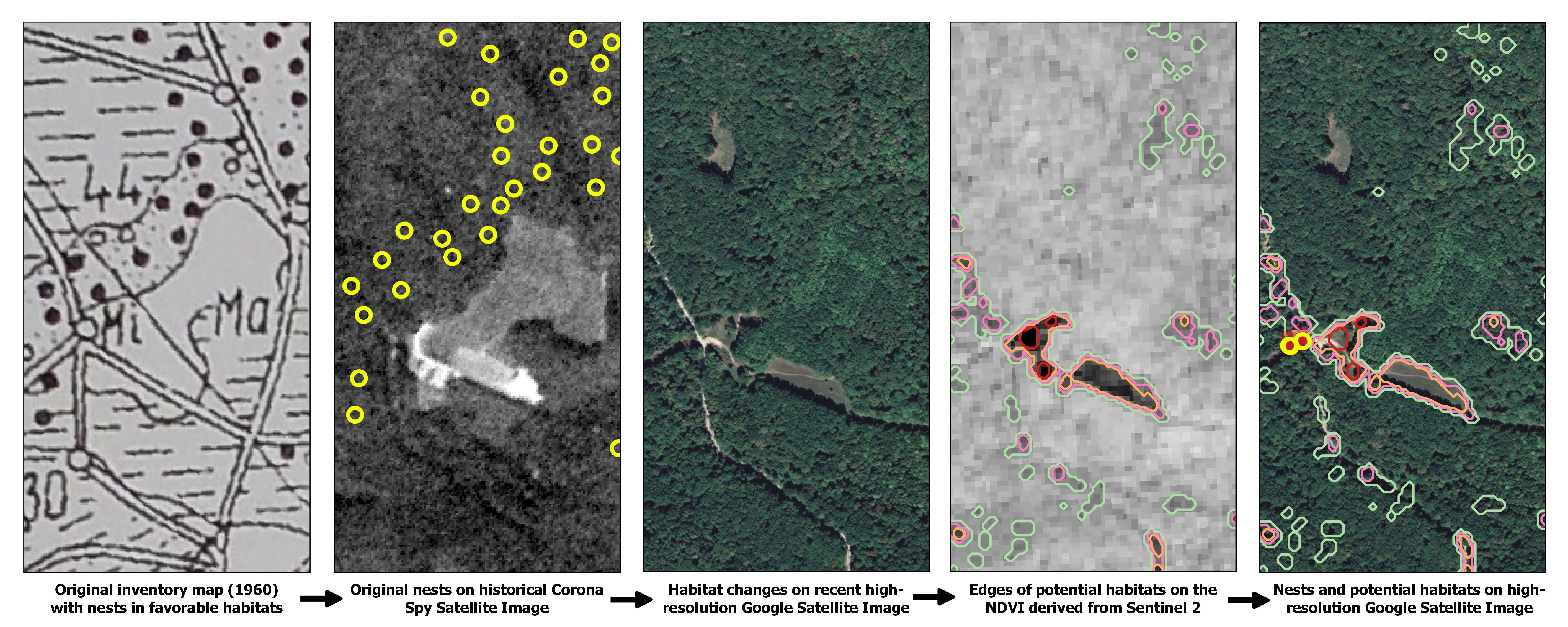
The study site is located in the hill region of Northeastern part of Romania, approximately 16 km SE of the city of Iasi near the village Poieni (County of Iasi) in a state-owned forest (Figure 1). Altitudes range from 190 to 420 (mean 316) m a.s.l. and slopes between 3 and 28 (mean 8) degrees; all types of aspect are quite uniformly represented, the N NE E S and SW each covering roughly 14–18 % while the SE W and NW each cover 8% of the area [28]. Mean annual values for temperature are 8.7 °C and 593 mm for precipitation [29]. The site conditions favor deciduous pure and mixed forests dominated by European beech (Fagus sylvatica L.) and oaks (Quercus robur L., Q. petraea (Matt.) Liebl.) together with many other hardwoods. Besides these types of forests that dominate the study area, very few artificially planted coniferous stands (spruce Picea abies (L.) Karst., black pine Pinus nigra Arn., Scots pine P. sylvestris L., and larch Larix decidua Mill.) are present on very small areas. The forest is under active management: mostly shelterwood in the natural deciduous stands and clearcutting in hybrid poplar artificial plantations or for restoring the natural composition in the case of degraded stands. As a result, habitat conditions, especially canopy closure and height, are changing frequently. In terms of tree species composition, at the time of the 1960 inventory, the area was a hardwood forest dominated by oak-beech mixed stands of medium or higher productivity, as well as beech mixed with other deciduous species along with some conifers, namely spruce, pine, and larch, artificially planted in small patches [9].
2.2. Nest Inventory and Statistical Analysis
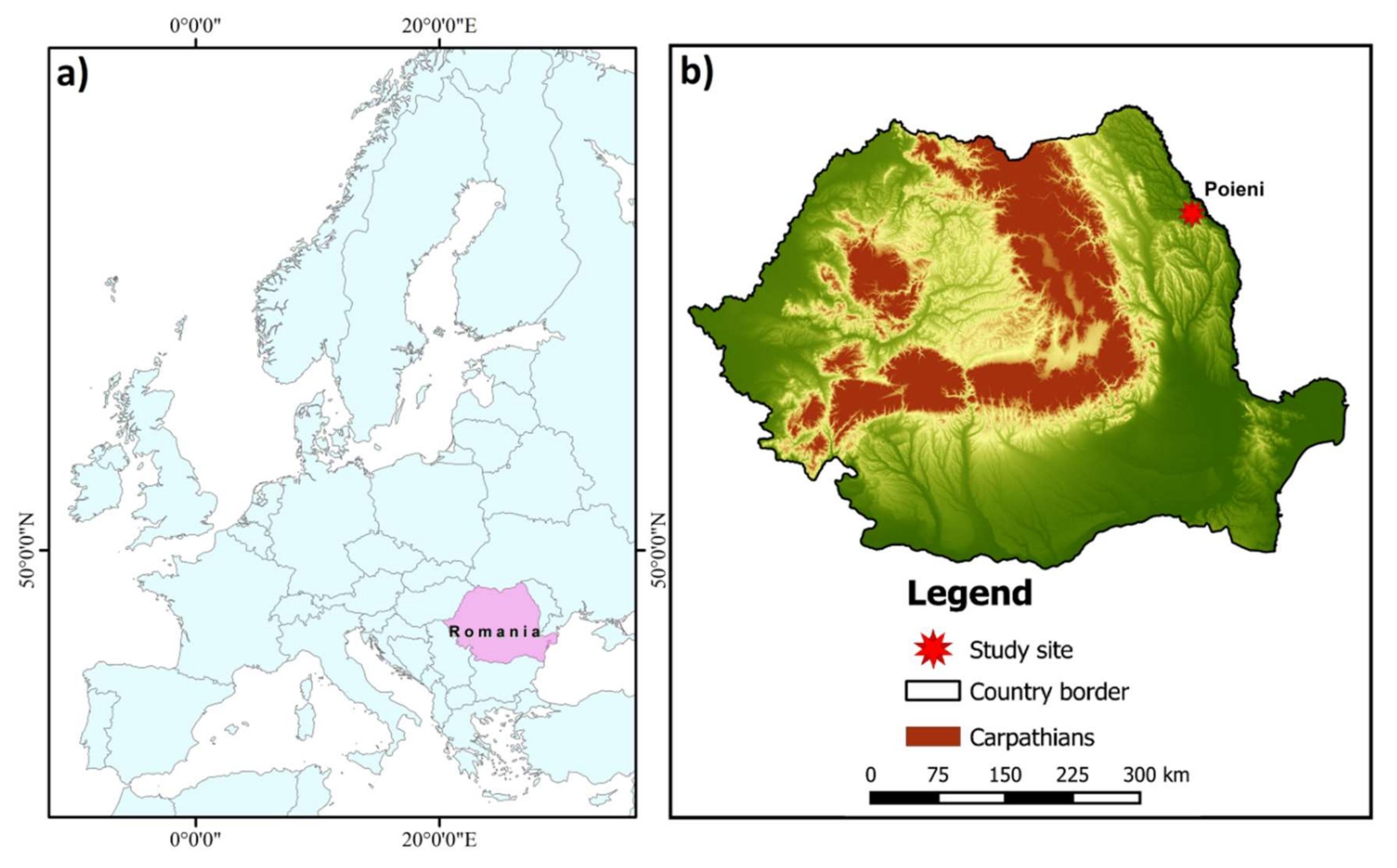
For 1960, a forest management plan map with the hand drawn position of the nests was available (Figure 2) with species names taken from Gösswald [30]. The accompanying text [11] gives a full list of synonyms referring to Betrem [31] and Yarrow [32], including the presently still valid designations:
Formica rufopratensis minor syn. Formica polyctena Först. 1850;
Formica rufopratensis major syn. Formica rufa L. 1761 (presumably as oligogynous small nest groups);
Formica rufa rufa syn. Formica rufa L. 1761 (presumably as typical monogynous single nests);
Formica nigricans syn. Formica. pratensis Retz. 1783.
Beside these, Formica (Serviformica) fusca Forel, a so-called “slave ant” for dependent colony foundation by young Formica gynes, was also described in the original text [11], but no clear reference was provided on its presence in the study area and no position shown on the original map (Figure 2).
All nests from the original 1960 map (Figure 2) were transformed to vector as points. Before carrying out any spatial analyses on nest position, the old map was visually checked against a rectified aerial Corona satellite image from 1964 [33]. Although the external border of both 1960 hand drawn old map and 1975 topographical map (1:25.000, DTM Romania) was consistent, we found inconsistencies concerning stand borders, valleys, and roads inside the map. Most probably, such details were hand drawn on the original map while the outer edge was derived from a topographical survey. Where such inconsistencies occurred, they have led to a relative misplacement of the RWA nests compared to their true location. For example, nests positioned on both sides of a road appeared to be located only on one side of this feature or, in the case of nests on an open border between stands, they seemed located further inside or outside the stand. In such cases, the individual clusters of nests were manually shifted (“backdating”-[34]) on a case-by-case basis on the high-resolution Google Earth satellite image [35]. Shifting was done based on their position relative to a certain spatial feature (e.g., road, valley, or crop border) from original stand map, to comply with the true position of these spatial features.
For the recent distribution of RWA nests, field inventories were carried out between 2016 and 2018 (hereinafter referred to as 2018). To complete this task, the available map with mound distribution in 1960 was first processed and uploaded to GPS handheld devices. The study site was then systematically thoroughly surveyed during the active months, always with three of the authors as experienced observers [36], at the beginning joined by local foresters, who explained peculiarities of the terrain and stand structure. As far as the terrain made it possible, we searched the investigation area in strips, the width of which were adapted to the stocking and visibility to avoid bias and to cover all site and stocking information. Nests were mapped using GPS tablet and Garmin handheld units (models GPSMap 60 & 62 and Oregon 550). Only active nests with a minimum diameter > 20 cm were considered. Apparently failing nests were also counted but only when workers were present (i.e., came out after carefully slightly knocking on the mound for verification).
Since the 1960 RWA data [11] are available by species separately for the single forest stands, but not for each nest, a summary treatment of the F. rufa-group was originally planned. Nevertheless, we repeatedly checked species identity during our inventories in the field with an illuminable 20x magnifying glass. For species-specific evaluation, we systematically collected 4–7 workers directly from the RWA mound surface, covering the entire area of distribution in the field. A total of 130 nests (i.e., approximately 30%) were sampled. Species were determined on mounted dry samples in the lab using Seifert’s key [37] using a variable up to 120 times magnification stereomicroscope OLYMPUS SZ and subsequently a LEICA M165C plus the live measurement module from Leica Microsystems (Leica Application Suite LAS X software) for counting and measuring pilosity [38].
All georeferenced data were incorporated into an ArcGIS 10.6 [39] respectively QGIS 3.4 [40] database and analyzed using Matlab [41] and R [42]. A point pattern analysis was carried out on the RWA distribution, using three different functions: the Ripley’s K function (K), the nearest-neighbor function (G), and the empty-space function (F). Although all three can be used to assess clustering, the method behind each is different. The K-function gives, for each nest, the average number of neighbor nests lying within a certain distance divided by the density of nests per unit area. The G-function analyzes the distance to the nearest neighbor while the F-function analyzes the distance from a fixed point to the nearest neighbor [43]. To compensate for potential edge effect bias (i.e., not including in analysis potential nests located outside the study area but close to the edge) for each function, three different edge correction methods were used: border correction, isotropic correction, and translation correction for Ripley’s K-function (K); Kaplan–Meier, border correction, and Hanisch for the nearest-neighbor function (G); and Kaplan–Meier, border correction, and Chiu-Stoyan for the empty-space function (F) [43]. Besides, a nearest neighbor and cluster analysis was carried out in ArcGIS, using the Anselin Local Morans I- and the Getis-Ord Gi*-statistics [44,45]. As nests in 1960, compared to the GPS-inventory in 2018, had been positioned on the map by hand, the precision of their position is lower. However, we would expect that any potential clustering would be still detectable for the original dataset as well.
2.3. Habitat Assessment
2.3.1. Initial Habitat
Besides information from the contemporary management plan, a 1964 Corona satellite image [33] was used to assess the original spatial forest conditions in the study area. To correct for error given by topographical and lens distortion, we used orthorectification based on structure from motion [26]. To improve the initial precision (26.4 m) based on 15 control points, this image was then rectified in ArcMap based on 67 ground control points using a spline transformation which reduced the error to 1.5 m.
On the rectified Corona image, we assessed the presence of habitat conditions that could favor the high number and spatial clustering of RWA nests. We aimed at identifying the following types of places:
- those adjacent to permanent forest edges (e.g., to road, agricultural areas or grassland);
- those adjacent to temporary forest edges (between e.g., young/short and old/tall forest). This also includes the case of open borderlines between stands. Even if such lines were narrow, enough radiation could penetrate to the ground at least at young ages, since trees with smaller heights cannot overshadow such lines. If trees forming the edge have less dense crowns (e.g., oaks, pines, larch), conditions will remain open longer;
- those inside or adjacent to stands with more open canopies. In such cases, the habitat would be permanent if the canopy is more open due to species (e.g., oaks), or temporary if it is due to recent silvicultural works (e.g., thinning) or age of stand (i.e., before reaching canopy closure).
Considering these types of edges, we checked their presence in areas where nests had been identified in 1960. Such places were transformed to vector as lines for roads and other types of linear edges, and to polygons in the case of young conifer plantations and recent regenerated areas. Since the Corona image did not always provide sufficient detail, or in places that had low quality, maps from the forest management plans 1966 were additionally used to extract permanent roads as well as open boundary lines and edges between forest types, small/tall stands, grasslands/agricultural fields, tree nurseries, etc. Further, these places were validated on the Corona image rendered as single band pseudocolor. A general assessment of habitat conditions was also carried out on the original 1960 map and a list of stand categories was created (Table A2) based on the information from its map legend and affiliated literature [9,10,11]. Finally, the position of nests in relation to existing edges and boundaries in their vicinity was visually checked and verified.
2.3.2. Recent Habitat
In 2018, the forest on the study site included species which provide very dense canopies, not allowing enough solar radiation to reach ground (e.g., beech, hornbeam, linden, walnut, spruce) as well as species with light, permeable crowns offering good radiation conditions (e.g., oaks, wild cherry, ash, willows, poplars, sycamore, larch, pines). Many times, such species mix. Therefore, we assessed present habitat conditions by extracting forest management plan information on tree species composition (as a surrogate for the general light regime). Each stand was classified as either “shade canopy” or “light canopy”, if proportion of species producing high shade respectively those allowing light to penetrate was at least 80% each and as “mixed canopy” when the proportion of each of the categories was at least 30%. Based on this classification, a map with potential habitat, i.e., “shaded”, “mixed”, and “light” stands was produced.
Moreover, as the forest is under active management, thinning is frequently carried out and favorable conditions can be present even in stands dominated by or totally composed of species that produce dense shade. Therefore, potential habitat for ants could be widely distributed across the forest, additionally depending both on forestry works, e.g., tending operations (especially thinning), openings in the canopy produced by shelterwood, or by sanitation cuttings (removal of trees damaged by disturbances), but also on construction of roads or stand boundary open lines, providing all kinds of edges influencing light availability. Therefore, a table with the number of forestry works carried out during the last decades in the stands with nests was compiled and the distribution of RWA nests analyzed. This method (easier and faster) provided information on tree species and effects of management activities on crown cover, but no spatially explicit distribution of gaps or portions of canopy with different types of crowns. Therefore, for the 2018 habitat types, we additionally used recent high-resolution satellite images to assess canopy cover and density and specially to detect the actual spatial distribution of canopy openings. In order to carry out this analysis, we produced a Normalized Difference Vegetation Index (NDVI) classified image using Google Earth Engine and Sentinel 2 repository, which was imported in QGIS [40]. We then separated categories of stand canopy cover on the NDVI [46]. The thresholds between categories were set using a Jenks optimization method [47], which is a data clustering method designed to determine the best arrangement of values into different classes (i.e., seeking to reduce the variance within classes and maximize the variance between classes). Further, based on visual interpretation between high-resolution Google Earth satellite image [35] and the 2018 Sentinel 2 satellite image (and taking into account known points from the field), results were optimized. The following classes resulted:
- −1 < NDVI < 0.5336 = open area, far away from edge;
- 0.5336 < NDVI < 0.6115 = shaded open area near edge, outside the stand;
- 0.6115 < NDVI < 0.6375 = the edge of the forest;
- 0.6375 < NDVI < 0.6634 = well-lit area near edge, inside the stand;
- 0.6634 < NDVI < 1 = closed, dense canopy, inside stand, far from edges.
Next, using “Reclassify values (simple)”-function, based on a Lookup Table, the QGis program has produced the NDVI classified image. On the resulting map, based on their preferences for solar radiation known from literature, RWA habitat categories 2, 3, and 4 were considered as being “RWA suitable”, i.e., offering intermediate conditions for solar radiation. Categories 1 (open area) and 5 (closed, dark stands) were considered “not RWA suitable”, representing extreme conditions, with either excessive or not enough solar radiation. Next, on the NDVI raster image, nests falling inside categories “RWA suitable” were separated from those falling outside. For the latter (i.e., nests falling in categories 1 and 5), we then analyzed the distance from nest to the edge of the nearest “RWA suitable” category. To complete this task, we extracted the contours of RWA habitat categories 2 to 4 from the validated raster, using the function Contour (in QGIS). These contour lines represent the boundaries between subsequent categories of RWA habitat. Using the function v.distance (in QGIS), we measured the distance for each of these nests to the nearest contour line. We used a threshold distance of 30 m, corresponding to the range around the nests in which the RWA mostly concentrate their activity, effectively capturing more than 50% of forest pests and where the density of honeydew producing aphids is significantly increased [16,48,49,50]. A distance threshold (supported by literature) rather than a mound size threshold was used as nest size (including workers number) varies over time (and thus, the size of the territory the nest is able to control varies accordingly). Nests located within the 30 m threshold distance were considered in “RWA suitable” habitat. Cases with more than 30 m were checked on the high-resolution Google Earth satellite images to assess for the presence of small gaps producing edges not detected on the NDVI. Such missed gaps were validated and manually added into the layer and the distance analysis was repeated.
3. Results
3.1. RWA Distribution Pattern
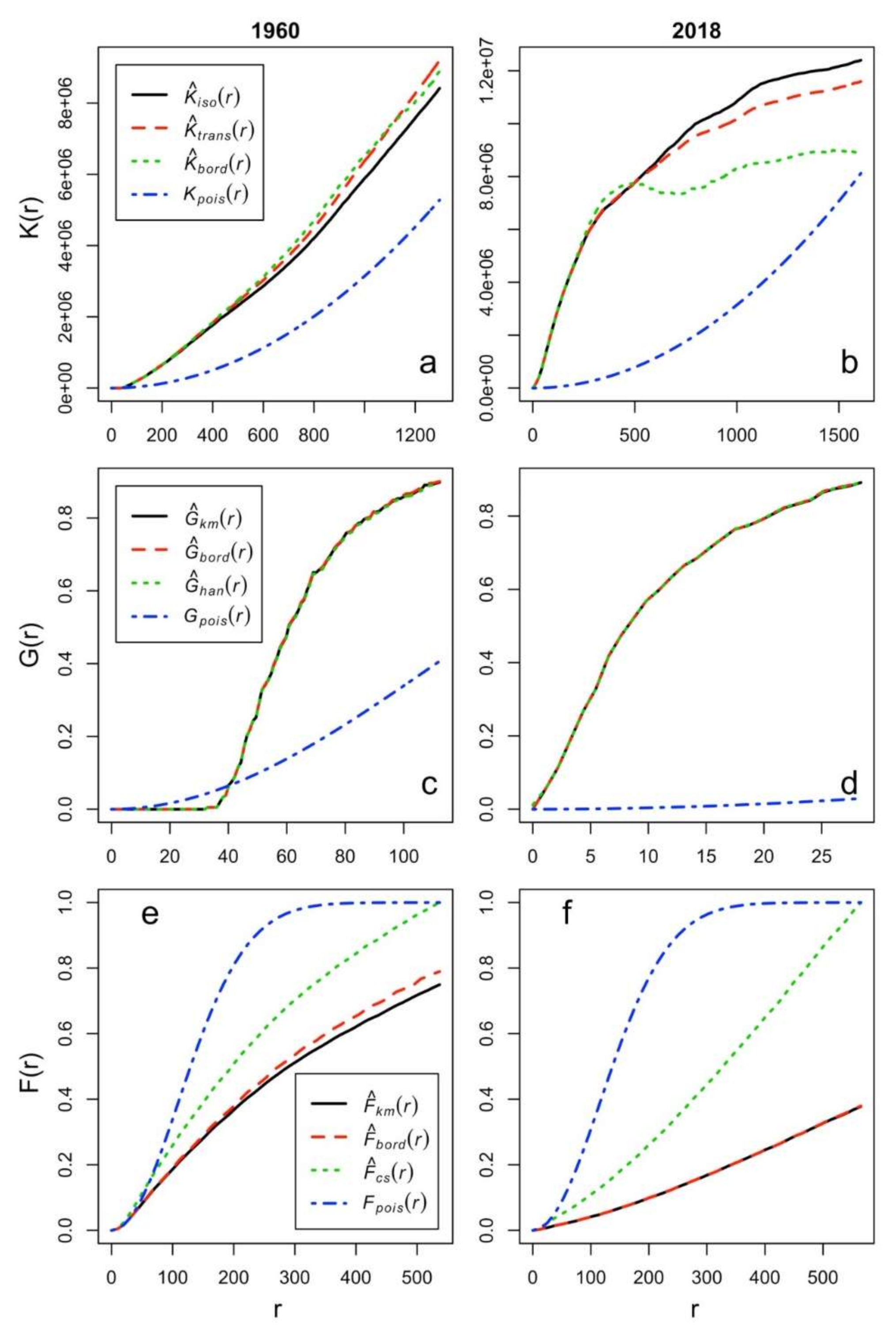
According to the point pattern analysis, despite the lower positioning precision in the original inventory (since nests had been hand drawn on map in 1960), the RWA distribution was not random but spatially clumped at both inventories. All three different spatial correlation functions (Figure A1) showed clear deviations from a random, theoretical Poisson distribution, indicating a clustered pattern.
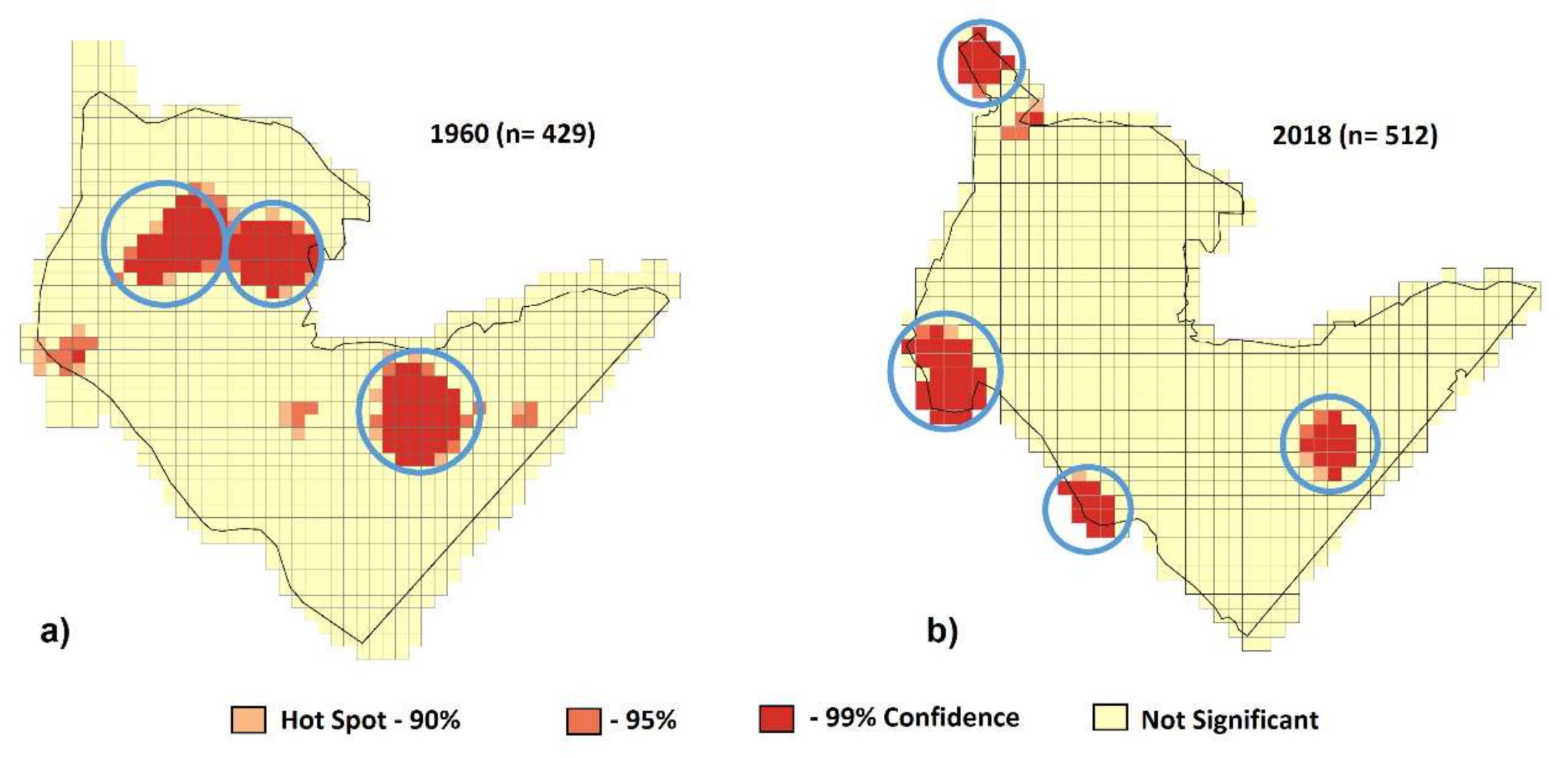
The original distribution in 1960 consisted of three major aggregations (Figure A2a) where all three actually valid Formica species were represented, mostly in and around coniferous stands, as well as looser associations and more scattered nests in the deciduous forest (Figure A3). The nearest neighbor analysis also underlined the strong clustering of RWA (high negative scores—Table A1), which formed statistically significant hotspots. There was a clear delimitation between high-density and ant-free areas. The large mean inter-nest distance observed in 1960 could partly be related to positioning the nests on the original hand drawn map. Of the 1960 location with three aggregations, only one had remained in the same location (although significantly reduced) in 2018, but three new ones (clumped significantly closer) had developed, resulting in a total of four aggregations with an average of 108 nests each (Figure A2b). Thus, distribution type was clustered at both inventories, but the number of mounds forming aggregations was significantly higher in 2018 (84%) than in 1960 (42%).
3.2. RWA Distribution and Habitats
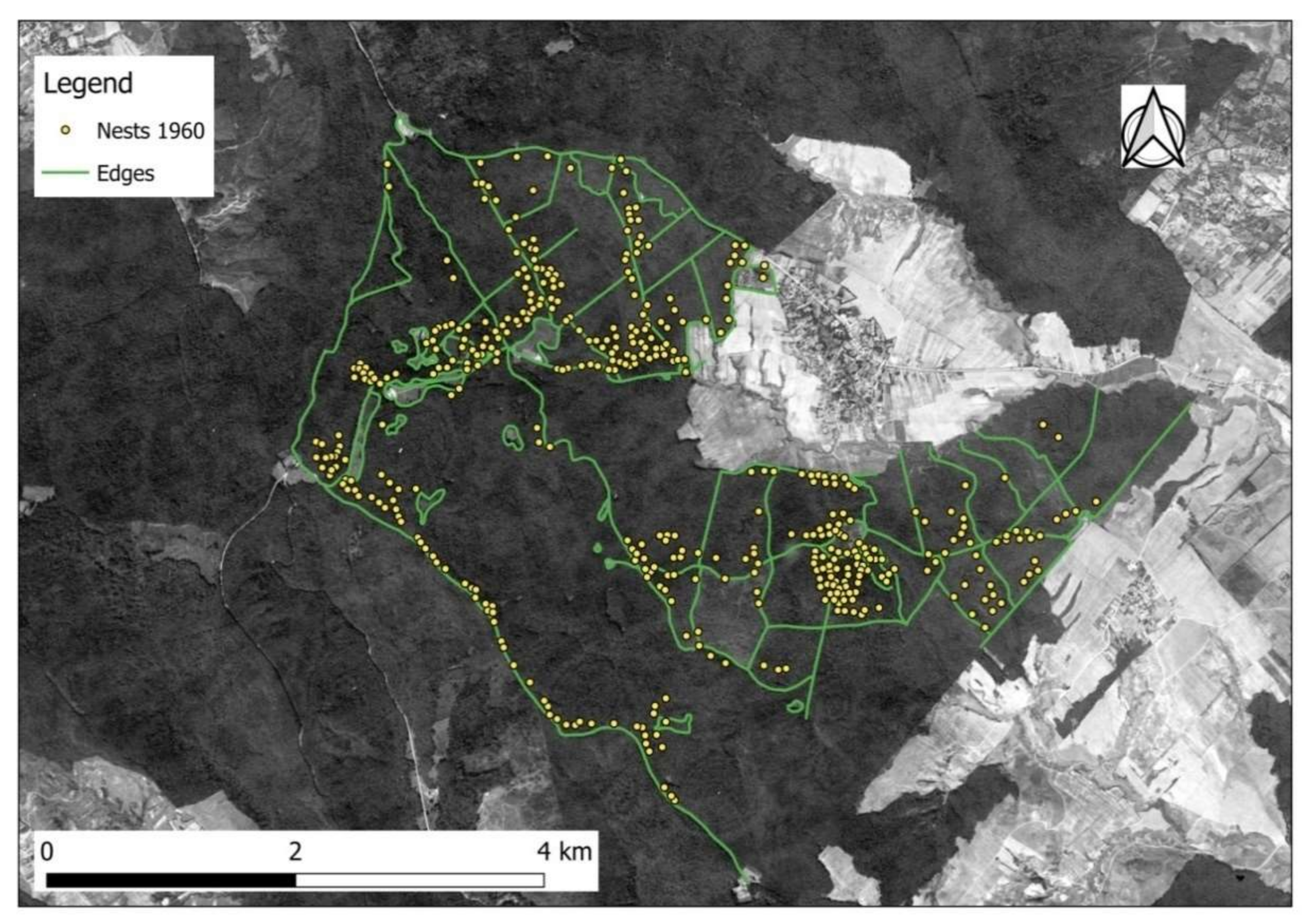
The RWA inventory carried out in 1960, on the entire 1868.0 ha, had revealed a total of 429 active nests. They amounted to a mean density of 23 nests per 100 ha (Table A2). Derived from the representation in Figure 2, F. rufa predominated in the southern half of the study area, presumably the old-named F. rufa rufa with 1 queen only (monogynous) single nests (monodomous) and old-named F. rufopratensis major with few queens (oligogynous) in small nest groups (oligodomous). F. polyctena clearly had its focus in the northern half of the study area, while F. pratensis only occurred in one single location. According to the forest stands differentiated in 1960, the RWA were centered within the few conifer patches established outside of their natural range through plantations (Figure A3). Hardwoods were most likely to contain RWA in oak-dominated stands, but less where beech and hornbeam prevailed (Table A2). The position of the RWA mounds in 1960 was in most of cases in areas where favorable habitat was detected on the map (i.e., canopy cover provided intermediate shaded habitat). Such conditions were either where crowns were less dense (e.g., young plantations or naturally regenerated stands before canopy closure; stands of species with permeable crowns—Figure A3), or where edges (between smaller/taller stands; next to roads or openings/agricultural fields) were present (Figure 3).
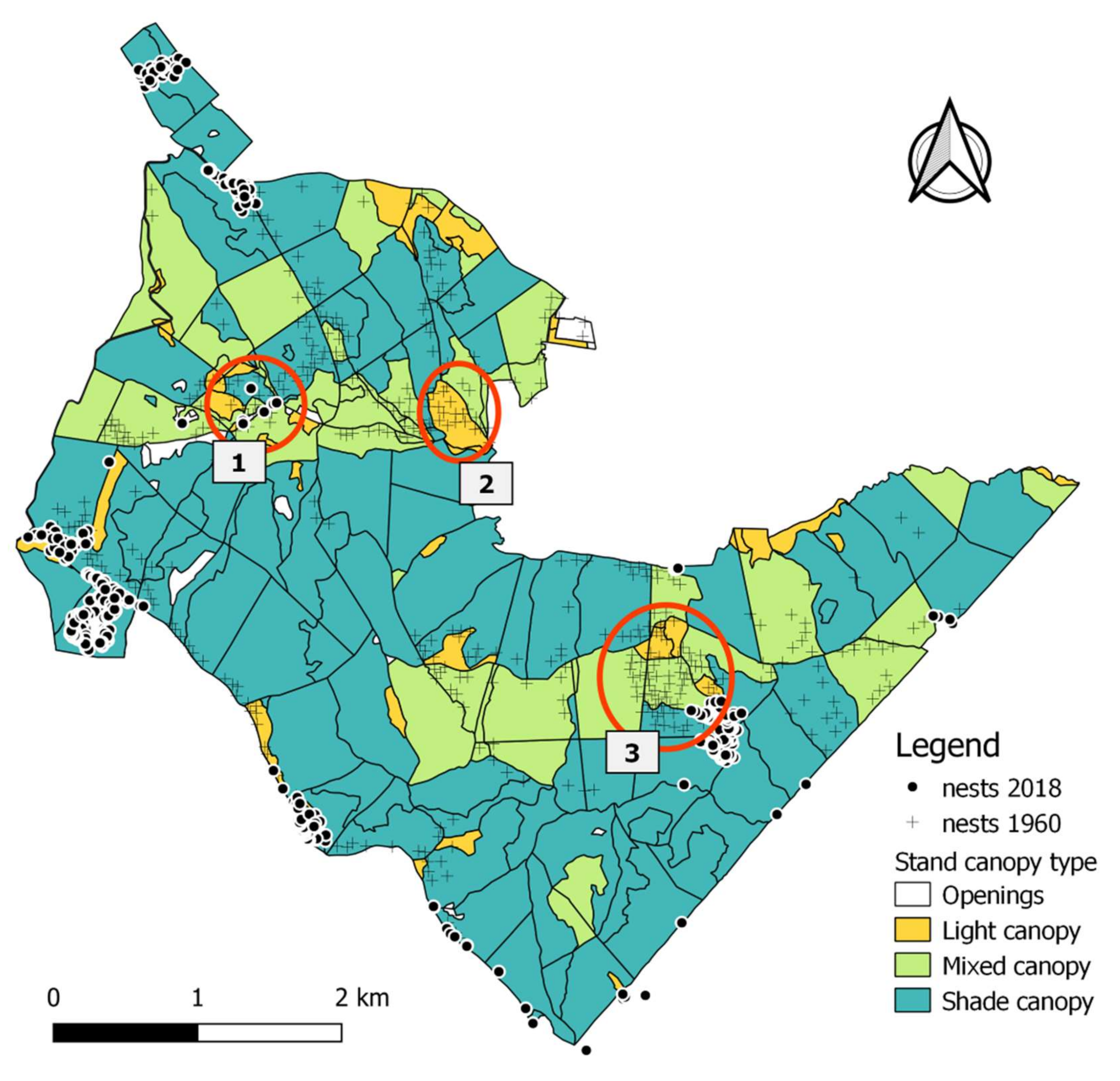
In 2018, we mapped a total of 512 active RWA nests: 346 on the original 1868.0 ha area plus a total of 166 additional nests in directly adjacent stands. The samples collected from the field for species identification were all identified in the laboratory as F. polyctena. While the 2018 RWA population was minimal in conifer stands, their densities were by far the highest in beech and hornbeam dominated stands, which should have a dense closed canopy (Figure 4). In terms of tree species composition in the hardwood stands, a significant shift had in fact occurred, switching towards shade tolerant tree species (71% of stands having a “shade canopy”) producing dense crowns (Table A3). Many of the former RWA nests had vanished from areas where stand conditions yet seemed favorable, with composition still being dominated by light crown species (Figure 4).
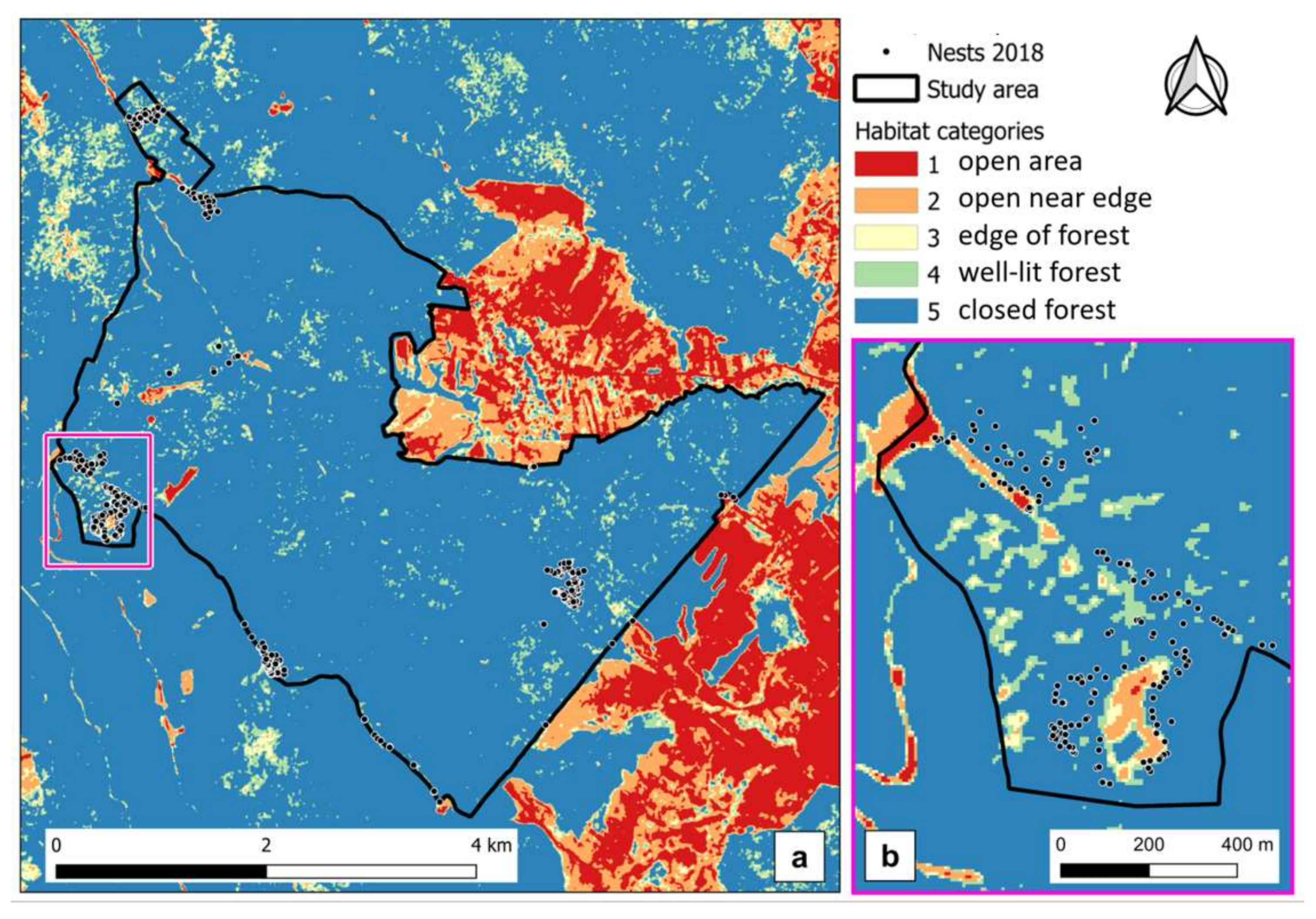
The subsequent analysis on stand canopy cover based on forest management plan information further clarified that, even if in beech stands, most of the nests were below relatively open canopy. Stands with canopy closure between 60–80% contained approximately 58% of RWA nest occurrence (Table A4). For stands with even more dense canopies (≥90%), the consideration of forestry works from the management plans demonstrated that beech and hornbeam canopy had in fact been opened by thinnings or other works such as sanitation cuttings, removal of trees damaged by disturbances, and therefore conditions for nests have become favorable. For approximately 30% of total RWA, at least two forestry works had been carried out recently in the stands with dense (≥90%) crown cover (Table A4). These results were confirmed by the additional analyses carried out on the produced NDVI map (Figure 5) which showed that 78 % of the 2018 nests (399 out of 512) were positioned in NDVI category 5 (representing dark and dense closed forest-Table 1).
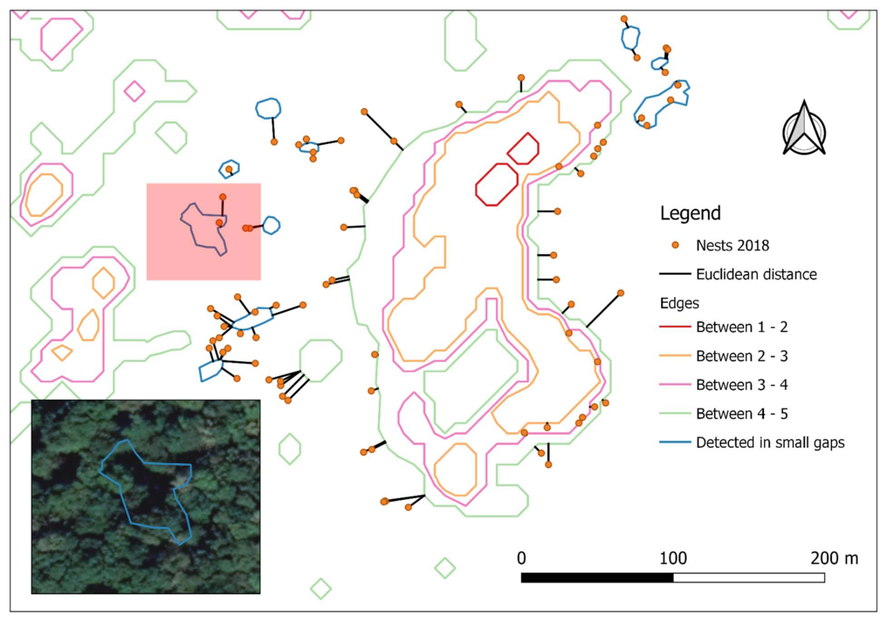
However, the analysis on the distance to a suitable habitat category showed that in most of the cases (306 out of 399), nests were located within less than 30 m from the edge of such habitat. Thus, 82% of all nests (419 out of 512) actually occurred either in places with adequate solar radiation conditions or closer than 30 m to such habitats. For all remaining 93 nests (18% of the total) located not only in extremely closed dense canopy stands (NDVI category 5) but also farther away than 30 m from edges of any of the NDVI categories 2 to 4, the analysis on Google Earth high-resolution satellite image showed that they were in fact in the vicinity of small canopy openings (Figure 6).
The validation on the Google Earth high-resolution satellite image of the gaps missed by the NDVI showed that all these 93 nests were indeed small clusters around 44 gaps of 237.5 m2 on average (ranging from 35.9 to 1300.7 m2). After these gaps were included in the “edge” shapefile and the measurement of distance to edge was repeated, all nests conformed to the 30 m distance from the edge of any of the suitable NDVI categories 2–4.
4. Discussion
4.1. Old Map and Satellite Image
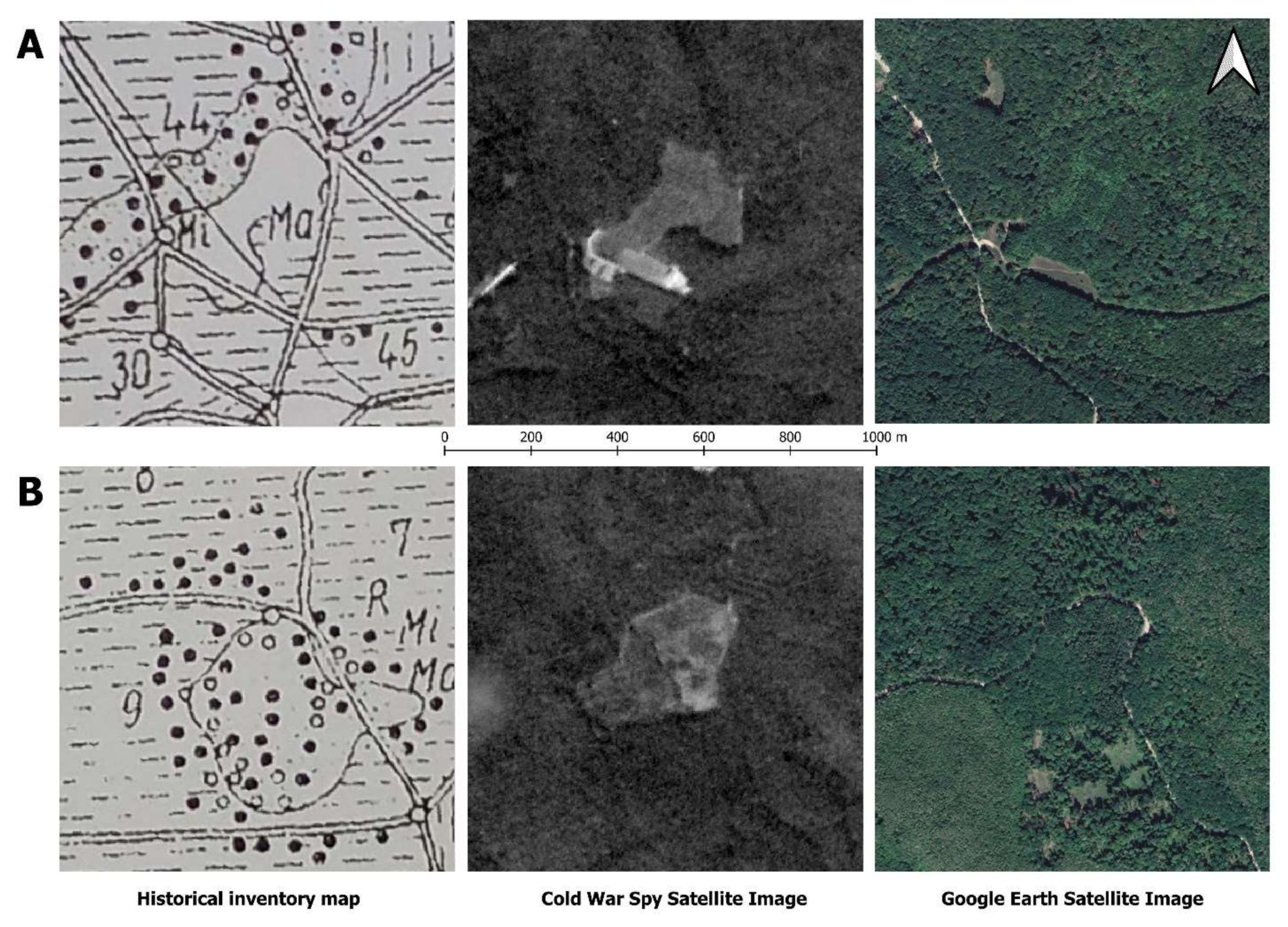
Our study expands approaches to evaluate the distribution of forest dwelling mound building RWA by better dealing with the limitations of former documents and maps of species occurrence. In our case, the original hand-drawn sketch had large points for nests and thereby distances larger than usual among them. Fortunately, this could be compensated for by a wealth of additional information from literature, forest management plans and especially old satellite images. This last source provided very important spatial information for rectifying the position of the old map, and consequently the distribution of nests. In addition, and even more important, it helped for the identification of edges (i.e., favorable habitats), reliably identified on Corona 1964 satellite image. Such conditions could provide beneficial conditions for RWA, since providing enough solar radiation. Moreover, the identification of certain features (roads, stand edges and adjacent agricultural fields) allowed for improving the location of the hand-drawn nests from the old map through “back-dating”. The existence of such data also allows for very valuable comparisons across time scales, showing the changes in habitat conditions (from more open to dense, closed stands; from existing edges to no edge–Figure 7).
4.2. Solar Radiation Regime
To guarantee sufficient light and heat to the RWA, access to solar radiation plays a crucial role [19]. However, light availability in forest ecosystems changes dramatically along stand development because of forest management or natural disturbances, providing for a shifting habitat availability in time. As a result, we should expect a changing spatial distribution of ants as well. RWA in our study confirmed this rule, their nests being located in certain canopy conditions, avoiding very closed, dark, and humid forests (where lack of radiation limits their existence), and also the fully open conditions (with restricted access to prey, particularly aphid trees). Indeed, in this study, no nests were found in fully open conditions, far from an edge. As for the case of very closed, dark, and humid forests, nests were only found close to a more open or fully open area. Nests located inside the stand far from edges did take advantage of a more open canopy due to species permeable crowns or recent natural or anthropogenic disturbances. Such particular situations allowed enough solar radiation to reach the ground, thereby offering similar conditions to the stand edge. Favorable conditions inside stands were therefore provided by intermediate canopy cover, which offers not only favorable environment for aphid colonies and potential prey but also allows enough radiation to penetrate to the ground, as shown in our study. Such conditions can persist in time along permanent edges or in stands of species with light crowns (e.g., pine, oaks) if (or until) no thick underbrush or dense young regeneration is installing underneath (after regeneration cuttings or natural disturbances). However, inside stands dominated by species providing dense shade (e.g., beech, hornbeam), the availability of favorable habitat conditions is more dynamic. Habitat became periodically available due to disturbances or management activities, which improve the radiation regime at forest floor [51]. After the canopy became too dense again in such forests, RWA did persist in the area, but only near edges with more open environments.
4.3. Changes in Habitat Suitability
A continuously shifting light regime in forest structure under natural regime or management will sometimes favor RWA colonies and at other times limits their presence [52]. At the first inventory in 1960, the RWA clearly preferred conifer plantations, where quite a bit of light was penetrating the canopies, since they were not yet closed. In 2018, however, we found a pronounced shift to broadleaves, mostly due to reduction of the site-inappropriate conifers. While RWA are generally considered to avoid hardwoods [53], such occurrence is common in Romania [52,54,55]. In our study, RWA were usually close to adjacent openings such as canopy gaps, roads, forest boundaries, or grasslands. Some former edges and open sub-compartment lines have vanished as trees had grown tall and crowns closed the canopy above them. In addition, in one of the light-demanding conifer stands, a dense underbrush is now present. These changes (which heavily influenced the light regime) forced ants to move out. However, where edges were permanent, e.g., roads or forest boundaries, the RWA colonies did maintain their location for decades. Figure 7 presents two such cases:
- an area formerly open in the 1960s, with clear edge and presence of nests, inside the nearby stand, which is now covered by a tall and dense stand (which has closed the edge previously offering favorable conditions) (Figure 7A);
- an area freshly planted with conifers in the 1960s, with open canopy and with evident edges towards surrounding stands (offering good conditions inside and around the edge). The area is now covered by a dense stand (dark canopy, no edges). Below, a previously closed dense stand (in the 1960s) now provides better conditions (access to more radiation) being opened by regeneration cuttings (Figure 7B).
4.4. Changes in Ant Species
From Figure 2, an approximate reconstruction of the RWA species present at that time is possible. The original distribution in the 1960s was dominated by F. polyctena and F. rufa, with F. polyctena predominating in the north and F. rufa in the south of the study area. This applied in particular within the densely populated conifer stands. If we assume that our identification of the 30% of 2018 RWA nests is representative for the entire study area, then F. polyctena has displaced the earlier present F. rufa. This could be explained by the ecological differences between the two species (nesting properties such as number of queens per nest, nests per colony, and dispersal strategy) [56]. Between 1960 and 2018, the proportion of conifer stands decreased significantly. In contrast, the share of hardwoods had increased, in particular shade-tolerant species with their dense crowns. Compared to the mono- to oligogynous and mono- to oligodomous F. rufa, this undoubtedly favored the polygynous and polydomous F. polyctena. For the latter, the heat balance in its large nests is more independent of external thermal conditions and thus enables the colonization even of darker and cooler habitats [37].
4.5. Classification of Stands
The use of forest management plan information to classify stands based on canopy types (“light”, “mixed”, or “shaded”) based on tree species composition (Table A3) provides only a general and broad estimation of suitable RWA habitats. Sometimes this could be effective, such as in the case of the shaded spruce plantation (Figure 4: circle 1), which is now mature and therefore too dark for maintenance of the former RWA aggregation, which has vanished. However, at other times, this can be misleading as in the case of nests formerly present in light demanding pines and larches. Here, despite the more open stand canopy, nests had vanished because of newly developed dense underbrush, which severely limits the light reaching the ground (Figure 4: circle 2). Moreover, ants can take advantage of small patches of favorable conditions not detectable by this method. Therefore, a general stand level classification of canopy types, which corresponds to relative proportion of tree species, can miss many and diverse potential habitats. Such a general classification does not provide information on the distribution of light-crown species inside shade crown species dominated stands, or on spatial position of gaps or proximity of edges (i.e., presence of potentially suitable habitats). This explains the contradicting situation from Table A3 where most of the nests are located in “shade canopy” stands, which supposedly do not offer favorable conditions. The additional information provided by management plans on relatively recent forestry works helped explain this contradiction. It showed that indeed canopy of such stands was more open (i.e., habitat was more favorable—Table A4) due to management, at least temporarily. The case of the newly installed small startups located in shade tolerant deciduous forest (Figure 4: in the S-E outside of circle 3) confirmed this as well. They have installed after a recent thinning, when radiation became available (but due to the recent management and not due to tree species). The additional use of the NDVI classified image provided a spatially characterization of crown closure and explained this strong settlement in apparently dense stands (Table A4). However, this method is not sufficient for very small-scale analyzes.
Overall, using the information from the forest management plans referring to either the general crown closure, species composition or forestry works carried in the past has an important limitation: it does not provide information on the presence and spatial location of favorable habitats inside stand (especially the small-scale ones—gaps or permeable canopies) or nearby (edges, roads, etc.).
4.6. Satellite Images and Derived Products
The analysis on the NDVI derived image overcame the drawbacks of the above-mentioned method based on information from forest management plans. This new method provided a spatially explicit distribution of canopy gaps inside forests. Such gaps were not detectable on the old satellite map and on the stand maps derived from species composition or canopy closure. Therefore, it helped identify the favorable habitat for RWA not only in terms of size (detecting small-scale gaps) but also in terms of its spatial location. It successfully showed that around 80% of the nests fell either inside the RWA suitable habitat categories 2 to 4 or within the 30 m distance to such favorable habitats (offering the RWA access to more solar radiation and trees to forage or visit aphid colonies). However, for nearly 20% of RWA, small gaps still providing favorable habitat inside dense closed stands were not detected on the NDVI. They were masked by the casted shade (i.e., therefore values of NDVI ranged from 0.66 to 0.76, erroneously indicating a closed canopy). This was due to the 20 m pixel size of Sentinel 2 and points out that the sole use of NDVI for habitat classification can be affected by errors, especially when aiming at small-scale differentiation. However, the additional use of the Google Earth high-resolution satellite image helped to correct this limitation.
5. Conclusions
Besides competition, foraging efficiency, and parasitism, the actual distribution of our RWA is a response to a wide array of habitat variables among which solar radiation plays a major role. In our study area, the highly clumped distribution of the RWA at both inventories confirmed a very strong interaction between the RWA and their heterogeneous environment. The dynamics in forest structure in the last six decades, produced by stand development and forest management, changed the light regime, and thus directly influenced ant distribution. On the other hand, permanent or long-lasting edges (to roads, agricultural fields, and stand borderlines, etc.) provided continuous favorable conditions for long periods. Overall, the continued presence of similar numbers of ant nests in the study area (albeit for many cases in different places along time) confirms the functionality of the “shifting steady-state mosaic” produced under active forests management. Such a dynamic mosaic has provided a space-for-time substitution and ensured continuous habitat conditions for ants. It gives them the chance to move out when conditions become unfavorable but also to eventually return when conditions become favorable again. These findings make it clear that single inventories are not sufficient to cover the underlying causes of the site selection. Only long-term studies could reveal the great variability and plasticity of the RWA habitat requirements [57,58,59] and lead to a reliable catalog of management measures for a targeted promotion of the useful RWA.
In terms of assessing favorable habitat inside stands, as this study shows, not the tree species themselves (despite being host to prey and honeydew supplying aphid colonies for the RWA), but the resulting stand canopy closure is the key habitat feature. This parameter (influenced by tree species but also by forestry works) favored or limited the presence of nests (by providing or limiting the solar radiation needed by ants). Furthermore, this study shows that combining management plan data with the satellite image processing and analysis provides a reliable and expedite method for detecting the presence of favorable small-scale habitat. In our case it helped explaining the dynamics of the ant colonies in managed or natural forests. Compared to previous research (e.g., [27]), this research also proves the usefulness of the historical satellite images in very different areas and with different species. Therefore, such modern spatial techniques can be successfully used in ecological monitoring across very large landscapes and in different parts of the world, especially in the context of recent ecosystem dynamics driven by climate change.
Author Contributions
Conceptualization: literature overview and field investigation possibility, P.T.S. and M.P. Defining the objectives of the study, P.T.S., D.K., M.D.N. and M.P. Methodology: development of satellite image and NDVI analysis, D.K. and P.T.S.; field work and collecting protocols, P.T.S., D.K. and M.P. Formal analysis: GIS application and NDVI analysis, M.D.N., D.K. and P.T.S.; satellite image acquisition, M.D.N.; statistical analysis, P.T.S. and D.K. Investigation: field investigation (mapping/ant nest searching), D.K., P.T.S. and M.P.; RWA collection and field measurements, P.T.S. and M.P. Data curation: insect identification, D.K.; data analysis, M.D.N., P.T.S., M.P. and D.K. Forest data management, P.T.S. and M.P.; maps, figures, and graphs P.T.S., M.D.N. and D.K. Writing: original draft manuscript preparation and writing, P.T.S. and D.K. All authors have read and agreed to the published version of the manuscript.
Funding
Part of the fieldwork was financially supported by the following sources: research grant 8034/14.07.2017 (DRONSAT) funded by Transilvania University of Brașov, the project PN 19070204 granted by Romanian Minister of Research and Innovation, the exchange program between Transilvania University of Braşov (Romania) and Albert-Ludwigs-University of Freiburg (Germany) and the “Guest at Transilvania University” Program funded by Transilvania University of Brașov.
Acknowledgments
We thank F. Fornoff from the Chair of Nature Conservation and Landscape Ecology at University of Freiburg for his support in RWA identifications with the LEICA system. The authors would like to thank the National Forest Administration ROMSILVA (Iasi County Branch–Forest Districts Ciurea and Dobrovăț) for granting access and guidance in the field and support with relevant information from the forest management plans. The authors also express their gratitude to the journal “Revista Pădurilor” for permission to reproduce Figure 2. The useful suggestions and comments provided by the anonymous reviewers are also greatly appreciated.
Conflicts of Interest
The authors declare no conflict of interest.
Appendix A
Figure A1.
Results of point pattern analysis for RWA nests mapped in 1960 (left) and 2018 (right). (K = Ripley’s K function (a,b); G= the nearest-neighbor function (c,d); F = the empty-space function (e,f); „pois” = random, theoretical distribution Poisson; „bord” = border correction; „iso” = isotropic correction; „trans” = translation correction; „km” = Kaplan-Meier correction; „han” = Hanisch correction; „cs” = Chiu-Stoyan correction). The pattern shows clustering as [44]: -the curve for the empirical K-function is clearly above the theoretical curve (valid for a completely random pattern), showing that a nest has more neighbors than expected (when the pattern would be completely random);-for the G-function (which is interpreted in a similar manner to the K-function), the curve for the empirical data is above the theoretical curve (valid for a completely random pattern) and shows that the nearest-neighbor distances are shorter than expected under a random pattern;-for the F-function, the interpretation is opposite. The empirical curve is below the theoretical one meaning that empty-space distances are larger than expected in a random pattern.

Figure A2.
Location of RWA hotspots (blue circles) in 1960 (a) and 2018 (b).

Figure A3.
Distribution of RWA (n = 429) from 1960, in different types of forest stand from original Poieni map.
Figure A3.
Distribution of RWA (n = 429) from 1960, in different types of forest stand from original Poieni map.


Table A1.
Nearest Neighbor Analysis of RWA in 1960 and 2018, each calculated for the whole study areas as outlined.
Table A1.
Nearest Neighbor Analysis of RWA in 1960 and 2018, each calculated for the whole study areas as outlined.
| Inventory Year | 1960 | 2018 |
|---|---|---|
| Observed Mean Distance (m) | 72.8 | 18.8 |
| Expected Mean Distance (m) | 123.0 | 114.7 |
| Nearest Neighbor Ratio | 0.5919 | 0.1639 |
| z-score | −16.178 * | −36.207 * |
| number of nests | 429 | 512 |
* significance at p ≤ 0.0005
Table A2.
RWA nest numbers and densities per 100 ha from 1960 in different types of forest stands (compiled from Pascovici [9,11]).
| Forest Stand Categories | Forest Stand Sub-Categories | Area (ha) | No. of Nests | Density (Nests/100 ha) |
|---|---|---|---|---|
| F. sylvatica and diverse hardwood species | Fagus sylvatica & Carpinus betulus mixed stands | 229.50 | 45 | 20 |
| TOTAL | 229.50 | 45 | 20 | |
| Pure Q. robur forests | Pure Q. robur stands on plateaus of medium productivity | 23.76 | 8 | 34 |
| TOTAL | 23.76 | 8 | 34 | |
| Mixed forests with Q. petraea & F. sylvatica of medium respectively high productivity | Mixed hardwood stands (F. sylvatica & Q. petraea most abundant) of high productivity | 112.44 | 15 | 13 |
| Mixed hardwood stands (F. sylvatica & Q. petraea most abundant) of medium productivity | 1320.03 | 214 | 16 | |
| TOTAL | 1432.47 | 229 | 16 | |
| Mixed forests with Q. robur & Q. petraea & F. sylvatica of medium productivity | Mixed hardwood stands (Q.robur & Q. petraea most abundant) of medium productivity | 26.88 | 8 | 30 |
| Mixed hardwood stands dominated by Q. petraea of medium productivity | 50.76 | 38 | 75 | |
| Mixed hardwood stands dominated by Q. robur of medium productivity | 34.45 | 26 | 76 | |
| TOTAL | 112.09 | 72 | 64 | |
| Artificial and semi-artificial standsof conifers with some hardwoods | Plantations of conifers (Larix decidua, Pinus sylvestris & Picea abies) and Q. petraea | 9.00 | 25 | 278 |
| Plantations of Picea abies, Pinus sylvestris and diverse hardwood species | 9.02 | 36 | 400 | |
| Pure Picea abies plantations | 2.54 | 7 | 276 | |
| Young hardwood plantations (<10 year.) | 50.08 | 7 | 14 | |
| TOTAL | 70.64 | 75 | 106 | |
| GRAND TOTAL | 1868.46 | 429 | 23 | |
Table A3.
Distribution of RWA in 2018 according to type of canopy derived from tree species composition (cf. text).
Table A3.
Distribution of RWA in 2018 according to type of canopy derived from tree species composition (cf. text).
| Type of Canopy | Area (ha) | Proportion of Area (%) | Number of Nests | Proportion of Nests (%) |
|---|---|---|---|---|
| Open grounds | 25.7 | 1.3 | 5 | 1.0 |
| Light canopy | 95.1 | 4.7 | 12 | 2.3 |
| Mixed canopy | 472.5 | 23.1 | 26 | 5.1 |
| Shade canopy | 1446.3 | 70.9 | 469 | 91.6 |
| Total | 2039.6 | 100.0 | 512 | 100 |
Table A4.
Distribution of RWA in 2018 according to stand canopy cover and number of forestry works carried out in the last decades within the stands with ant nests.
Table A4.
Distribution of RWA in 2018 according to stand canopy cover and number of forestry works carried out in the last decades within the stands with ant nests.
| Canopy Cover (%) | Proportion of Nests (%) | Total (%) | ||
|---|---|---|---|---|
| Number of Forestry Works | ||||
| 0 | 1 | ≥2 | ||
| 0 | 1.0 * | 0.0 | 0.0 | 1.0 |
| 20 | 0.0 | 0.0 | 0.2 | 0.2 |
| 60 | 0.0 | 0.0 | 4.4 | 4.4 |
| 70 | 0.0 | 0.4 | 8.0 | 8.4 |
| 80 | 0.2 | 13.1 | 32.0 | 45.3 |
| 90 | 9.3 | 1.8 | 27.8 | 38.9 |
| 100 | 0.0 | 0.0 | 1.8 | 1.8 |
| Total | 10.5 | 15.3 | 74.2 | 100.0 |
* Five nests were located on the edge of the stands but have been associated by the GIS software to the open areas adjacent to the stands.
References
- Heinrichs, J.A.; Bender, D.J.; Schumaker, N.H. Habitat degradation and loss as key drivers of regional population extinction. Ecol. Modell. 2016, 335, 64–73. [Google Scholar] [CrossRef]
- Fischer, J.; Lindenmayer, D.B. Landscape modification and habitat fragmentation: A synthesis. Glob. Ecol. Biogeogr. 2007, 16, 265–280. [Google Scholar] [CrossRef]
- Watt, A.S. Pattern and process in the plant community. J. Ecol. 1947, 35, 1–22. [Google Scholar] [CrossRef] [Green Version]
- Kimmins, J.P. Forest Ecology: A Foundation for Sustainable Forest Management and Environmental Ethics in Forestry, 3rd ed.; Prentice Hall: Upper Saddle River, NJ, USA, 2004; ISBN 9780130662583. [Google Scholar]
- Agosti, D.; Majer, J.; Alonso, L.E.; Schultz, T. Ants: Standard Methods for Measuring and Monitoring Biodiversity; Agosti, D., Majer, J., Alonso, L.E., Schultz, T., Eds.; Smithsonian Institution Press: Washington, DC, USA; London, UK, 2000. [Google Scholar]
- Underwood, E.C.; Fisher, B.L. The role of ants in conservation monitoring: If, when, and how. Biol. Conserv. 2006, 132, 166–182. [Google Scholar] [CrossRef]
- Ellison, A.M. Out of Oz: Opportunities and Challenges for Using Ants (Hymenoptera: Formicidae) as Biological Indicators in North-Temperate Cold Biomes. Myrmecological News. 2012. Available online: https://dash.harvard.edu/bitstream/handle/1/8519155/Ellison_2012_OutofOz.pdf (accessed on 28 January 2021).
- Ribas, C.R.; Campos, R.B.F.; Schmidt, F.A.; Solar, R.R.C. Ants as indicators in Brazil: A review with suggestions to improve the use of ants in environmental monitoring programs. Psyche 2012, 2012, 636749. [Google Scholar] [CrossRef] [Green Version]
- Pașcovici, V. Contribuții la problema combaterii biologice în păduri cu ajutorul furnicilor—Inițierea unor cercetări în masivul păduros Poieni-Iași. Rev. Pădurilor 1961, 76, 295–299. (In Romanian) [Google Scholar]
- Pașcovici, V.; Simionescu, A.; Podariu, M.; Pentiuc, V.; Caraman, V. Cercetări Privind Furnicile de Pădure din R.S. România și Folosirea lor în Combaterea Dăunătorilor Forestieri; Editura Silvica: Ilfov, Romania, 1968. (In Romanian) [Google Scholar]
- Pașcovici, V. Combatere Biologică cu Ajutorul Furnicilor din Genul Formica, L. (Hymenop. Formicidae) și Necesitatea Utilizării ei în R.P.R.: Inițierea unor Cercetări în Masivul Păduros Poieni-Iași; Ministerul Agriculturii, Ed.; Editura Agro-Silvică: Bucharest, Romania, 1961. (In Romanian) [Google Scholar]
- Sorvari, J.; Hakkarainen, H. Forest clearing and sex ratio in forest-dwelling wood ant Formica aquilonia. Naturwissenschaften 2007, 94, 392–395. [Google Scholar] [CrossRef]
- Grevé, M.E.; Hager, J.; Weisser, W.W.; Schall, P.; Gossner, M.M.; Feldhaar, H. Effect of forest management on temperate ant communities. Ecosphere 2018, 9, e02303. [Google Scholar] [CrossRef]
- Wellenstein, G. Zur Frage der Standortansprüche. hügelbauender Waldameisen (Formica rufa-Gruppe). Z. Angew. Zool. 1967, 54, 139–166. [Google Scholar]
- Procter, D.S.; Cottrell, J.; Watts, K.; Robinson, E.J.H. Do non-native conifer plantations provide benefits for a native forest specialist, the wood ant Formica lugubris? For. Ecol. Manag. 2015, 357, 22–32. [Google Scholar] [CrossRef] [Green Version]
- Sudd, J.H.; Douglas, J.M.; Gaynard, T.; Murray, D.M.; Stockdale, J.M. The distribution of wood-ants (Formica lugubris Zetterstedt) in a Northern English forest. Ecol. Entomol. 1977, 2, 301–313. [Google Scholar] [CrossRef]
- Kilpeläinen, J.; Punttila, P.; Finér, L.; Niemelä, P.; Domisch, T.; Jurgensen, M.F.; Neuvonen, S.; Ohashi, M.; Risch, A.C.; Sundström, L. Distribution of ant species and mounds (Formica) in different-aged managed spruce stands in eastern Finland. J. Appl. Entomol. 2008, 132, 315–325. [Google Scholar] [CrossRef]
- Chen, Y.-H.; Robinson, E.J.H. The relationship between canopy cover and colony size of the wood ant Formica lugubris—Implications for the thermal effects on a keystone ant species. PLoS ONE 2014, 9, e116113. [Google Scholar] [CrossRef] [PubMed]
- Kadochová, Š.; Frouz, J. Red wood ants Formica polyctena switch off active thermoregulation of the nest in autumn. Insectes Soc. 2014, 61, 297–306. [Google Scholar] [CrossRef]
- Punttila, P.; Kilpeläinen, J. Distribution of Mound-Building Ant Species (Formica spp., Hymenoptera) in Finland: Preliminary results of a national survey. Ann. Zool. Fenn. 2009, 46, 1–15. [Google Scholar] [CrossRef] [Green Version]
- Reymond, A.; Purcell, J.; Cherix, D.; Guisan, A.; Pellissier, L. Functional diversity decreases with temperature in high elevation ant fauna. Ecol. Entomol. 2013, 38, 364–373. [Google Scholar] [CrossRef]
- Del Toro, I.; Berberich, G.M.; Ribbons, R.R.; Berberich, M.B.; Sanders, N.J.; Ellison, A.M. Nests of red wood ants (Formica rufa-group) are positively associated with tectonic faults: A double-blind test. PeerJ 2017, 2017, e3903. [Google Scholar] [CrossRef] [Green Version]
- Niemelä, J.; Haila, Y.; Punttila, P. The importance of small-scale heterogeneity in boreal forests: Variation in diversity in forest-floor invertebrates across the succession gradient. Ecography 1996, 19, 352–368. [Google Scholar] [CrossRef]
- Véle, A.; Holuša, J.; Frouz, J. Ecological requirements of some ant species of the genus Formica (Hymenoptera, Formicidae) in spruce forests. J. For. Sci. 2009, 55, 32–40. [Google Scholar] [CrossRef] [Green Version]
- Kasimova, R.G.; Tishin, D.; Obnosov, Y.V.; Dlussky, G.M.; Baksht, F.B.; Kacimov, A.R. Ant mound as an optimal shape in constructal design: Solar irradiation and circadian brood/fungi-warming sorties. J. Theor. Biol. 2014, 355, 21–32. [Google Scholar] [CrossRef]
- Niță, M.D.; Munteanu, C.; Gutman, G.; Abrudan, I.V.; Radeloff, V.C. Widespread forest cutting in the aftermath of World War II captured by broad-scale historical Corona spy satellite photography. Remote Sens. Environ. 2018, 204, 322–332. [Google Scholar] [CrossRef]
- Munteanu, C.; Kamp, J.; Nita, M.D.; Klein, N.; Kraemer, B.M.; Müller, D.; Koshkina, A.; Prishchepov, A.V.; Kuemmerle, T. Cold War spy satellite images reveal long-term declines of a philopatric keystone species in response to cropland expansion. Proc. Biol. Sci. 2020, 287, 20192897. [Google Scholar] [CrossRef] [PubMed]
- NASA Jet Propulsation Laboratory. Shuttle Radar Topography Mission Global 1 Arc Second [Data Set]. Available online: https://www2.jpl.nasa.gov/srtm/ (accessed on 28 January 2021).
- Fick, S.E.; Hijmans, R.J. WorldClim 2: New 1-km spatial resolution climate surfaces for global land areas. Int. J. Climatol. 2017, 37, 4302–4315. [Google Scholar] [CrossRef]
- Gösswald, K. Rassenstudien an der roten Waldameise Formica rufa L. auf systematischer, ökologischer, physiologischer und biologischer Grundlage. Z. Angew. Entomol. 1941, 28, 62–124. [Google Scholar] [CrossRef]
- Betrem, J.G. Enkele opmerking ontrent de sorten van de Formica rufa-Groep (Hym.). Entom. Ber. 1953, 14, 322–326. [Google Scholar]
- Yarrow, I.H.H. The British ants allied to Formica rufa L.(Hym., Formicidae). Trans. Soc. Br. Entomol. 1955, 12, 1–48. [Google Scholar]
- U.S. Geological Survey. Declassified Intelligence Satellite Photographs: U.S. Geological Survey Fact Sheet 2008–3054; U.S. Geological Survey Earth Resources Observation and Science (EROS) Center: Sioux Falls, SD, USA, 2008. [Google Scholar]
- Kaim, D.; Kozak, J.; Kolecka, N.; Ziółkowska, E.; Ostafin, K.; Ostapowicz, K.; Gimmi, U.; Munteanu, C.; Radeloff, V.C. Broad scale forest cover reconstruction from historical topographic maps. Appl. Geogr. 2016, 67, 39–48. [Google Scholar] [CrossRef]
- Google Maps Poieni, Iasi Area. Available online: https://www.google.com/maps/@47.0309215,27.6454192,14z (accessed on 18 March 2020).
- Berberich, G.M.; Dormann, C.F.; Klimetzek, D.; Berberich, M.B.; Sanders, N.J.; Ellison, A.M. Detection probabilities for sessile organisms. Ecosphere 2016, 7, e01546. [Google Scholar] [CrossRef]
- Seifert, B. The Ants of Central and North Europe; Lutra: Tauer, Germany, 2018. [Google Scholar]
- Roquer-Beni, L.; Rodrigo, A.; Arnan, X.; Klein, A.M.; Fornoff, F.; Boreux, V.; Bosch, J. A novel method to measure hairiness in bees and other insect pollinators. Ecol. Evol. 2020, 10, 2979–2990. [Google Scholar] [CrossRef] [Green Version]
- Environmental Systems Research Institute (ESRI). ARCGIS Desktop, Version 10.6; Environmental Systems Research Institute: Redlands, CA, USA, 2016. [Google Scholar]
- QGIS Geographic Information System. OSGeo QGIS 3.4. Available online: http://qgis.osgeo.org2019 (accessed on 28 January 2021).
- The MathWorks Inc. Matlab2017 (R2010a); The MathWorks Inc.: Natick, MS, USA, 2017. [Google Scholar]
- R Core Team. R. A Language and Environment for Statistical Computin; R Foundation for Statistical Computing: Vienna, Austria, 2018; Available online: https://www.gbif.org/tool/81287/r-a-language-and-environment-for-statistical-computing (accessed on 18 March 2020).
- Baddeley, A.; Rubak, E.; Turner, R. Spatial Point Patterns: Methodology and Applications with R, 1st ed.; CRC Press: Boca Raton, FL, USA, 2015; ISBN 9781482210200. [Google Scholar]
- Ord, J.K.; Getis, A. Local spatial autocorrelation statistics: Distributional issues and an application. Geogr. Anal. 1995, 27, 286–306. [Google Scholar] [CrossRef]
- Getis, A.; Ord, J.K. The analysis of spatial association by use of distance statistics. In Advances in Spatial Science; Springer: Cham, Switzerland, 2010; Volume 61, pp. 127–145. [Google Scholar]
- Gamon, J.A.; Field, C.B.; Goulden, M.L.; Griffin, K.L.; Hartley, A.E.; Joel, G.; Penuelas, J.; Valentini, R. Relationships between NDVI, canopy structure, and photosynthesis in three Californian vegetation types. Ecol. Appl. 1995, 5, 28–41. [Google Scholar] [CrossRef] [Green Version]
- Jenks, G.F. The data model concept in statistical mapping. Int. Yearb. Cartogr. 1967, 7, 186–190. [Google Scholar]
- Wellenstein, G. Die Beeinflussung der forstlichen Arthropodenfauna durch Waldameisen (Formica rufa-Gruppe). Z. Angew. Entomol. 1957, 41, 368–385. [Google Scholar] [CrossRef]
- Wellenstein, G. Waldbewohnende Ameisen, ihre Bedeutung, ihre Biologie, ihre Hege und ihr Schutz, 2nd ed.; Allgäuer Zeitungsverlag GmbH: Kempten, Germany, 1990. [Google Scholar]
- Gordon, D.M. The development of an ant colony’s foraging range. Anim. Behav. 1995, 49, 649–659. [Google Scholar] [CrossRef] [Green Version]
- Palladini, J.D.; Jones, M.G.; Sanders, N.J.; Jules, E.S. The recovery of ant communities in regenerating temperate conifer forests. For. Ecol. Manag. 2007, 242, 619–624. [Google Scholar] [CrossRef]
- Tăușan, I.; Dauber, J.; Trică, M.R.; Marko, B. Succession in ant communities (Hymenoptera: Formicidae) in deciduous forest clear-cuts—An Eastern European case study. Eur. J. Entomol. 2017, 114, 92–100. [Google Scholar] [CrossRef] [Green Version]
- Ellis, S.; Franks, D.W.; Robinson, E.J.H. Ecological consequences of colony structure in dynamic ant nest networks. Ecol. Evol. 2017, 7, 1170–1180. [Google Scholar] [CrossRef] [Green Version]
- Duma, I. The impact of red wood ants Formica rufa on the distribution of invertebrate fauna from the forest’s floor. Ann. West Univ. Timis. Ser. Biol. 2003, 5–6, 121–130. [Google Scholar]
- Berberich, G.M.; Klimetzek, D.; Paraschiv, M.; Stancioiu, P.T.; Grumpe, A. Biogeostatistics confirm: Even a low total number of red wood ant nests provide new information on tectonics in the East Carpathian Orogen (Romania). Ecol. Indic. 2019, 101, 486–500. [Google Scholar] [CrossRef]
- Perron, M.; Glanzmann, I.; Freitag, A. Habitatselektion von zwei Waldameisenarten (Formica rufa und F. polyctena). Schweiz. Z. Forstwes. 2019, 170, 32–39. [Google Scholar] [CrossRef]
- Klimetzek, D. Die Variabilität der Standortansprüche hügelbauender Waldameisen der Formica rufa-Gruppe (Hymenoptera: Formicidae). Mitt. Badischen Landesver. Naturkd. Nat. N.F. 1973, 11, 9–25. [Google Scholar]
- Klimetzek, D.; Kaiser, M. Zur Ökologie der Formica rufa-Gruppe. Waldhygiene 1995, 20, 243–254. [Google Scholar]
- Klimetzek, D. Population studies on hill building wood-ants of the Formica rufa-group. Oecologia 1981, 48, 418–421. [Google Scholar] [CrossRef] [PubMed]
Figure 1.
Geographic location of the study area (a) and position of the study site within Romania (b).
Figure 1.
Geographic location of the study area (a) and position of the study site within Romania (b).

Figure 2.
Map of 1960 Poieni inventory area with stand compartments and major roads, Red Wood Ants (RWA) positions shown as black dots (adapted from Pascovici [11], reproduced with kind permission of the journal “Revista Pădurilor”). (Currently valid Formica species names are: Mi = F. polyctena, Ma = F. rufa (presumably oligogynous), R = F. rufa (presumably monogynous), N = F. pratensis).

Figure 3.
Position of forest edges identified on the 1964 Corona spy satellite image and distribuTable 1960. RWA.
Figure 3.
Position of forest edges identified on the 1964 Corona spy satellite image and distribuTable 1960. RWA.

Figure 4.
Distribution of RWA in 2018 (n = 512) and canopy classification. Red circles refer to areas where unexpected changes in RWA settlement occurred (for details see Section 4.5).
Figure 4.
Distribution of RWA in 2018 (n = 512) and canopy classification. Red circles refer to areas where unexpected changes in RWA settlement occurred (for details see Section 4.5).

Figure 5.
Stand canopy cover categories produced on the NDVI map (a) and detailed view of section with RWA nests 2018 (b).
Figure 5.
Stand canopy cover categories produced on the NDVI map (a) and detailed view of section with RWA nests 2018 (b).

Figure 6.
Mapping of the edges between NDVI categories (1 = open area, far away from edge; 2 = shaded open area near edge, outside the stand; 3 = the edge of the forest; 4 = well-lit area near edge, inside the stand; 5 = closed, dense canopy, inside stand, far from edges), nest locations, and distances to the nearest edge of a suitable habitat (categories 2–4). Blue lines describe edges of the small gaps identified later on the Google Earth high-resolution satellite image and manually added to the layer before final analysis (Photo in lower left: detail with gap not identified on the NDVI but evident on Google Earth).

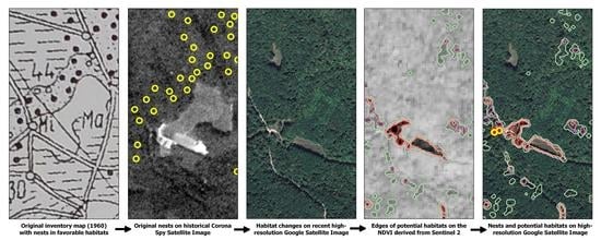
Figure 7.
Comparison of maps/images from different times (left = original hand-drawn map from 1960; middle = Corona spy-satellite image from 1960s; right = Google Earth satellite image). (A)—area formerly open in the 1960s, with clear edge and presence of nests nearby, inside the neighboring stand. At present closed, with very little edge left. (B)—former young, open canopy, conifer plantation in the 1960s. Now closed canopy, tall stand (no edges, no gaps).

Table 1.
Distribution of 2018 RWA according to canopy closure from the NDVI classification of RWA habitat categories.
Table 1.
Distribution of 2018 RWA according to canopy closure from the NDVI classification of RWA habitat categories.
| RWA Habitat Category | Area (ha) | Proportion of Area (%) | Number of Nests | Proportion of Nests (%) |
|---|---|---|---|---|
| (1) open area, far away from edge | 6.5 | 0.3 | - | - |
| (2) shaded open area near edge, outside the stand | 15.5 | 0.8 | 16 | 3 |
| (3) the edge of the forest | 19.7 | 1.0 | 31 | 6 |
| (4) well-lit area near edge, inside the stand | 97.2 | 4.8 | 66 | 13 |
| (5) closed, dense canopy, inside stand, far from edges | 1900.7 | 93.1 | 399 | 78 |
| Total | 2039.6 | 100.0 | 512 | 100 |
Publisher’s Note: MDPI stays neutral with regard to jurisdictional claims in published maps and institutional affiliations. |
© 2021 by the authors. Licensee MDPI, Basel, Switzerland. This article is an open access article distributed under the terms and conditions of the Creative Commons Attribution (CC BY) license (http://creativecommons.org/licenses/by/4.0/).
Share and Cite
MDPI and ACS Style
Klimetzek, D.; Stăncioiu, P.T.; Paraschiv, M.; Niță, M.D. Ecological Monitoring with Spy Satellite Images—The Case of Red Wood Ants in Romania. Remote Sens. 2021, 13, 520. https://doi.org/10.3390/rs13030520
AMA Style
Klimetzek D, Stăncioiu PT, Paraschiv M, Niță MD. Ecological Monitoring with Spy Satellite Images—The Case of Red Wood Ants in Romania. Remote Sensing. 2021; 13(3):520. https://doi.org/10.3390/rs13030520
Chicago/Turabian StyleKlimetzek, Dietrich, Petru Tudor Stăncioiu, Marius Paraschiv, and Mihai Daniel Niță. 2021. "Ecological Monitoring with Spy Satellite Images—The Case of Red Wood Ants in Romania" Remote Sensing 13, no. 3: 520. https://doi.org/10.3390/rs13030520
Note that from the first issue of 2016, this journal uses article numbers instead of page numbers. See further details here.