Joint Hapke Model and Spatial Adaptive Sparse Representation with Iterative Background Purification for Martian Serpentine Detection

Abstract

Visible and infrared imaging spectroscopy have greatly revolutionized our understanding of the diversity of minerals on Mars. Characterizing the mineral distribution on Mars is essential for understanding its geologic evolution and past habitability. The traditional handcrafted spectral index could be ambiguous as it may denote broad mineralogical classes, making this method unsuitable for definitive mineral investigation. In this work, the target detection technique is introduced for specific mineral mapping. We have developed a new subpixel mineral detection method by joining the Hapke model and spatially adaptive sparse representation method. Additionally, an iterative background dictionary purification strategy is proposed to obtain robust detection results. Laboratory hyperspectral image containing Mars Global Simulant and serpentine mixtures was used to evaluate and tailor the proposed method. Compared with the conventional target detection algorithms, including constrained energy minimization, matched filter, hierarchical constrained energy minimization, sparse representation for target detection, and spatially adaptive sparse representation method, the proposed algorithm has a significant improvement in accuracy about 30.14%, 29.67%, 29.41%, 9.13%, and 8.17%, respectively. Our algorithm can detect subpixel serpentine with an abundance as low as 2.5% in laboratory data. Then the proposed algorithm was applied to two well-studied Compact Reconnaissance Imaging Spectrometer for Mars images, which contain serpentine outcrops. Our results are not only consistent with the spatial distribution of Fe/Mg phyllosilicates derived by spectral indexes, but also denote what the specific mineral is. Experimental results show that the proposed algorithm enables the search for subpixel, low-abundance, and scientifically valuable mineral deposits.

1. Introduction

Recent advances in imaging spectrometer technology allow the simultaneous acquisition of hundreds of continuous spectral bands over the visible and infrared range [1,2,3]. The Compact Reconnaissance Imaging Spectrometer for Mars (CRISM) [3] conveys essential spectral information that is interpreted in order to determine the compositional and mineralogical makeup of the martian surface [4,5,6,7,8]. The characterized minerals are critical to understanding the evolution of Mars, which in turn serves as a potential window into our planet’s history. Many efforts have been made to map minerals regionally or globally on Mars based on hyperspectral images (HSIs) [9,10,11,12]. These studies reveal that Mars has a basaltic upper crust with regional variations in the relative abundances of other hydrated minerals [4].

Several methods have been developed to map martian minerals over the past decades. The most prevalent method uses spectral indices [13,14], which explore the position, depth, and shape of diagnostic absorptions to characterize minerals. Although this method has led to many significant findings, spectral indices could be ambiguous because an index may denote broad classes rather than a definitive specific mineral. In addition, due to insufficient spatial resolution and mixing effects happening at different spatial scales [15], mixed pixels are generally encountered in mineral mapping from orbit. To address the mixing phenomenon and acquire quantitative information of each constituent, a spectral unmixing technique is used on hyperspectral images of Mars [9,10,16]. However, the accuracy of abundance retrieval greatly depends on the selected endmembers [15]. Endmember extraction is challenging in CRISM data analysis due to relatively shallow spectral absorptions and spatial heterogeneity [17].

On Mars, scientists are more interested in the less exposed, sporadically distributed, but scientifically valuable hydrated minerals deposits compared with widely distributed basalts. Identification of these minerals can be regarded as a target detection process. Target detection focuses on distinguishing specific target pixels from various background pixels with a priori knowledge of the target spectra [18,19]. Recently, the sparse representation for target detection algorithm (STD) has attracted much attention [20,21,22,23]. The philosophy of STD is that a pixel in a HSI lies in a low-dimensional subspace and thus can be represented as a sparse linear combination of a structured dictionary consisting of target and background training spectral samples [21]. The target spectra are assumed to be known in advance, while the background dictionary is generated locally for each test pixel through a dual concentric window [21]. To further exploit the spatial information of HSI, the spatially adaptive STD (SASTD) [23] was proposed and achieved competitive performance. In essence, these representation theory-based methods are grounded in linear mixing modeling [19], which is unsuitable to mineral detection because the observed reflectance of mixtures involves nonlinear combinations of each endmember in visible and near infrared wavelengths [24]. Furthermore, the target interference with the background dictionary during the sliding process of the dual-window heavily degrades the detection performance [25].

Fortunately, single-scattering albedo (SSA) is linearly additive in visible and infrared wavelength [26]. The Hapke model relates a mineral mixture’s reflectance to a linear combination of the SSAs of its constituents [27]. To exploit the advantages of the representation theory-based method and make it suitable for mineral detection, we developed a nonlinear target detection framework by joining the Hapke model and SASTD (HSASTD). Moreover, an iterative background dictionary purification (IBP) strategy is proposed to mitigate the target interference issue. Before applying the proposed detection method to orbital data, we first rigorously tested the algorithm on an HSI acquired by a laboratory imaging spectrometer, which contains binary mixtures of serpentine and Mars Global Simulant (MGS-1). MGS-1 is a chemical and mineralogic analog to the martian basaltic regolith-specifically that of Rocknest measured by the Curiosity rover [28]. Six different mass fractions mixtures were prepared, namely 100%, 10%, 5%, 2.5%, 1%, and 0% serpentine. This dataset is used to evaluate and tailor the method to the unique qualities of serpentine. To sum up, the contributions of this paper are threefold.

• A joint Hapke model and spatially adaptive sparse representation approach was proposed for subpixel mineral detection. We address the nonlinear issue by introducing the Hapke model, which significantly boosts the detection performance. Furthermore, an iterative background purification strategy is proposed to alleviate the target interference issue, which can be easily implanted into other sparse representation detection algorithms;
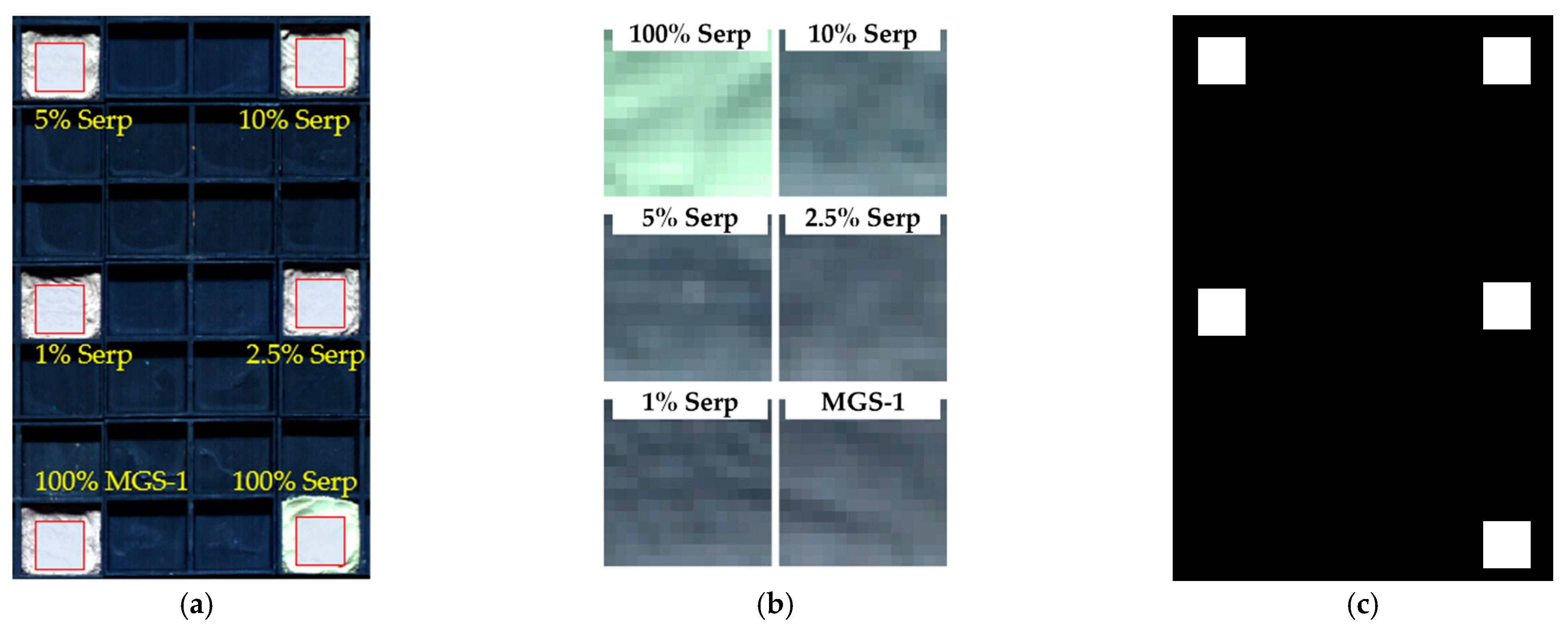
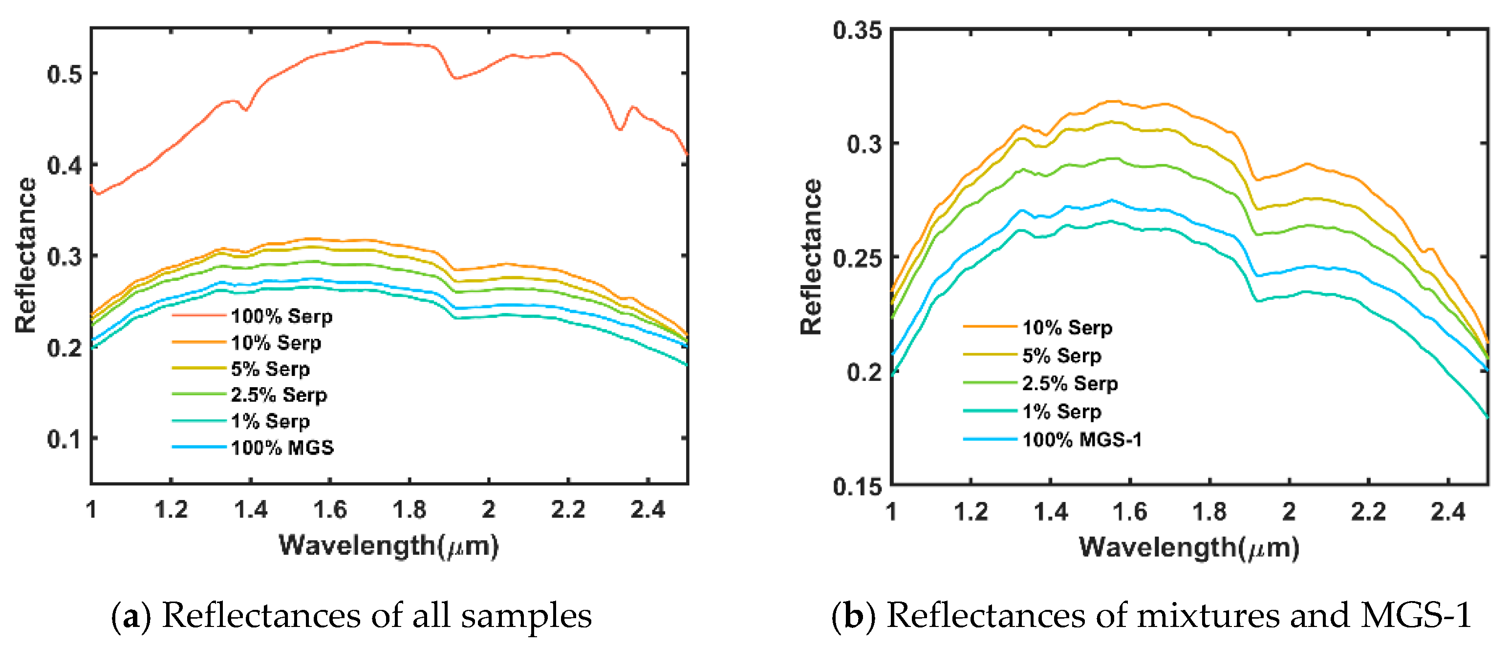
• We used a well-designed mineral mixture HSI to evaluate the detection capabilities of our method. The MGS-1 and serpentine were mixed by six different mass fractions to assess the detection performance of the proposed algorithm. This dataset includes detailed groundtruth information, which can serve as a benchmark dataset for martian mineral detection;
• A systematic comparison of several representative detection algorithms was conducted on the laboratory HSI. The detection limit of serpentine abundance by the proposed method was derived. Finally, the proposed method was applied to CRISM images. This study provides a critical link between laboratory measurement and orbital observation.

The rest of this paper is organized as follows. Section 2 briefly introduces preliminary knowledge of the martian mineral mapping methods and the STD. The datasets and the proposed algorithm are presented in Section 3. The experimental results of laboratory and CRISM HSIs are given in Section 4. The discussion and conclusions are covered in Section 5 and Section 6, respectively. Finally, a glossary of all the acronyms with brief descriptions is included in Appendix A.

2. Related Work

In this section, we first introduce two commonly used martian mineral mapping methods: spectral index and spectral unmixing. A detailed summary of spectral processing techniques for martian mineral mapping can be found in Supplement Table S1. Subsequently, the STD is briefly reviewed.

2.1. Martian Mineral Mapping Methods

Spectral Index: Spectral indexes use the position, depth, and shape of diagnostic absorptions to identify minerals [13,14].

Table 1. Compact Reconnaissance Imaging Spectrometer for Mars (CRISM) spectral indexes related to phyllosilicates.

Name	Meaning	Formulation [14]	Rationale	Caveats
BD1900	1.9 μm H2O band depth	$1-0.5\times \frac{R_{1930}+R_{1985}}{a\times R_{1850}+b\times R_{2067}}$	H2O
D2200	2.2 μm dropoff	$1-\frac{R_{2210}/R{C}_{2210}+R_{2230}/R{C}_{2230}}{2\times R_{2165}/R{C}_{2165}}$	Al-OH minerals	Chlorite, Prehnite
D2300	2.3 μm dropoff	$1-\frac{R_{2290}/R{C}_{2290}+R_{2320}/R{C}_{2320}+R_{2330}/R{C}_{2330}}{R_{2120}/R{C}_{2120}+R_{2170}/R{C}_{2170}+R_{2210}/R{C}_{2210}}$	Hydroxylated Fe, Mg silicates strongly > 0	Mg-Carbonate

shows several spectral indexes related to phyllosilicates. In the formulation, $R_{\mathsf{\lambda }}$ denotes the reflectance at wavelength $\lambda$. $R{C}_{\mathsf{\lambda }}$ represents the linear interpolated reflectance at $\lambda$, where $R{C}_{\mathsf{\lambda }}=a{R}_{{\mathsf{\lambda }}_{\mathrm{L}}}+b{R}_{{\mathsf{\lambda }}_{\mathrm{R}}}$, $b=({\lambda }_{\mathrm{C}}-{\lambda }_{\mathrm{L}})/({\lambda }_{\mathrm{R}}-{\lambda }_{\mathrm{L}})$, $a=1-b$, ${\lambda }_{\mathrm{L}}$ and ${\lambda }_{\mathrm{R}}$ are the wavelength at the left and right shoulder. Spectral indexes serve as guidelines for the assessment of a diverse range of minerals, such as phyllosilicates, carbonates, hydrated silica, and sulfates. To enhance the spectral contrast of the target mineral and mitigate the effects of the atmospheric correction residuals and instrumental artifacts, researchers usually divide the average spectrum of a region of interest (ROI) with a neutral spectrum from the same columns [7]. The ratioed spectrum is then compared with laboratory spectra. Although this method has led to many notable discoveries e.g., [5,7,8], the spectral index can be ambiguous because an index may denote broad classes rather than a specific mineral. Moreover, the selection of neutral spectra is often difficult and sometimes impossible, depending on the specific hyperspectral image. The hand-crafted nature of this method is time-consuming and inadaptable for extensive mineralogical surveys [29,30,31]. Recently, an exploratory mineralogical mapping method using CRISM spectral indexes was proposed to classify minerals [29]. However, the classification label often represents a mineralogical class rather than a specific mineral.

Spectral Unmixing: Spectral unmixing is also used in martian minerals mapping, which extracts the spectrally pure constituent materials and their respective fractional abundances in each mixed pixel. Mixing models can be categorized as either linear or nonlinear. Both linear [32,33,34] and nonlinear [9,16] unmixing models have been used to retrieve mineral abundances on Mars. In visible and near-infrared wavelengths, the observed reflectance of minerals is a nonlinear mixture of endmembers. The Hapke model [27] is a widely employed nonlinear mixing model for planetary spectral studies. However, the accuracy of abundance retrieval greatly depends on the selected endmembers. It is challenging to separate mineralogical information from instrument artifacts in the images because of the relatively shallow absorption features of surface minerals in orbitally acquired spectra [30]. Therefore, identifying all endmembers in the scene is nontrivial.

2.2. Sparse Representation for Target Detection

Unlike unmixing, which needs to determine all endmembers in the scene, target detection focuses on the target of interest, which intends to suppress the undesired background spectra and highlight the target spectra simultaneously. The characteristic of this approach is appropriate for identifying a specific spectral signature. Many target detection algorithms have been proposed over the last couple decades, such as statistical-based methods [35] and representation theory-based methods [18]. Among them, the STD algorithm has attracted much attention. The STD exploits the fact that a pixel in an HSI lies in a low-dimensional subspace and thus can be represented as a sparse linear combination of a structured dictionary [21]. In this work, the structured dictionary refers to a collection of target and background spectra. Let $y\in R^{\mathrm{L}}$ be a spectrum with $L$ bands, $D^{\mathrm{b}}$ and $D^{\mathrm{t}}$ are the background and target dictionaries consisting of $N^{\mathrm{b}}$ and $N^{\mathrm{t}}$ spectra. The spectrum $y$ can be linearly represented by multiplying the dictionary with a sparse vector as follows

$$\begin{array}{l}y=(D_1^{\mathrm{b}}{x}_1^{\mathrm{b}}+\dots +D_{N^{\mathrm{b}}}^{\mathrm{b}}{x}_{N^{\mathrm{b}}}^{\mathrm{b}})+(D_1^{\mathrm{t}}{x}_1^{\mathrm{t}}+\dots +D_{N^{\mathrm{t}}}^{\mathrm{t}}{x}_{N^{\mathrm{t}}}^{\mathrm{t}})\\ =[D_1^{\mathrm{b}}{D}_2^{\mathrm{b}}\dots D_{N^{\mathrm{b}}}^{\mathrm{b}}]{[x_1^{\mathrm{b}}{x}_2^{\mathrm{b}}\dots x_{N^{\mathrm{b}}}^{\mathrm{b}}]}^{\mathrm{T}}+[D_1^{\mathrm{t}}{D}_2^{\mathrm{t}}\dots D_{N^{\mathrm{t}}}^{\mathrm{t}}]{[x_1^{\mathrm{t}}{x}_2^{\mathrm{t}}\dots x_{N_t}^{\mathrm{t}}]}^{\mathrm{T}}\\ =D^{\mathrm{b}}{x}^{\mathrm{b}}+D^{\mathrm{t}}{x}^{\mathrm{t}}=Dx\end{array}$$

(1)

where $x^{\mathrm{b}}$ and $x^{\mathrm{t}}$ are vectors whose entries correspond to the coefficients of the columns in $D^{\mathrm{b}}$ and $D^{\mathrm{t}}$; $D\in R^{\mathrm{L}\times ({\mathrm{N}}^{\mathrm{b}}+{\mathrm{N}}^{\mathrm{t}})}$ is the union of background and target dictionary; $x\in R^{(N^{\mathrm{b}}+N^{\mathrm{t}})}$ is a concatenation of $x^{\mathrm{b}}$ and $x^{\mathrm{t}}$. The sparse vector $x$ can be derived by solving the following equation

$$x=\arg \min {\Vert x\Vert }_{0}s.t.{\Vert Dx-y\Vert }_2\le \delta$$

(2)

where ${\Vert x\Vert }_0$ denotes the ${\ell }_0$-norm, which is defined as the number of nonzero entries in x, σ is the fitting residual due to the noise and modeling errors. The equation in (2) can be solved by greedy pursuit algorithms. The recovery implicitly leads to a competition between the background and target subspaces [21]. The final detector is determined by comparing the reconstruction residuals between D^b and D^t.

$$f(y)=r_{\mathrm{b}}-r_{\mathrm{t}}$$

(3)

where $r_{\mathrm{b}}={\Vert y-D^{\mathrm{b}}{x}^{\mathrm{b}}\Vert }_2$, $r_{\mathrm{t}}={\Vert y-D^{\mathrm{t}}{x}^{\mathrm{t}}\Vert }_2$.

3. Datasets and Methodology

In this section, the laboratory and orbital HSIs are first described. Then, the proposed target detection method is illustrated in detail. The experimental settings and evaluation metrics are presented lastly.

3.1. Datasets

3.1.1. Laboratory Data

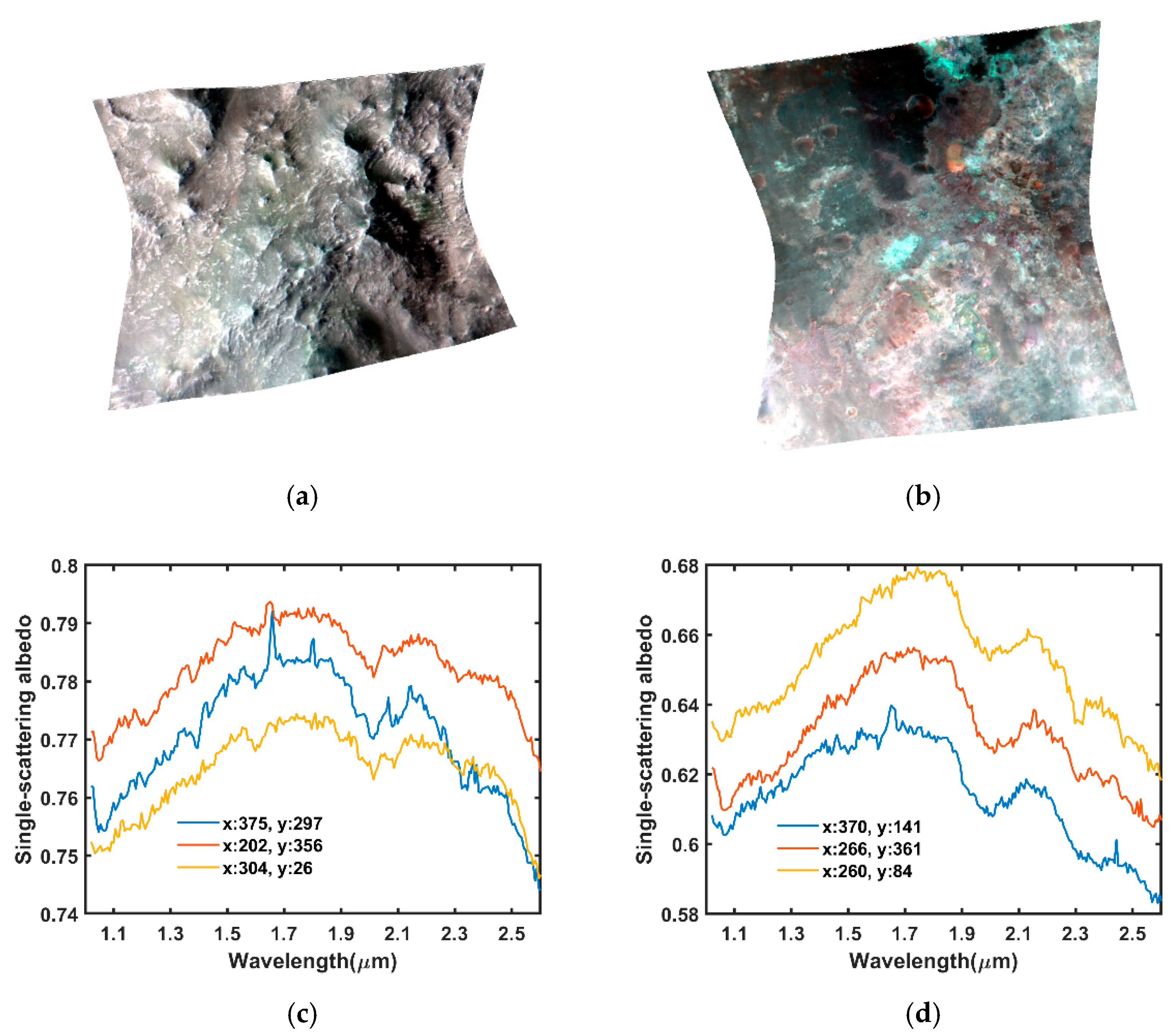
Samples preparation: Serpentine and MGS-1 powders were mixed by mass fraction in six proportions, precisely at 0%, 1%, 2.5%, 5%, 10% and 100% serpentine. The grain size of serpentine is dominated by 125~250 µm. The MGS-1 powders are sieved to <1 mm, which have a mean grain size of 122 µm [28]. The reason for selecting serpentine as an endmember is that serpentine serves as a marker for distinctive aqueous chemical conditions [36]. Its presence implies that localized habitable environments may have existed on ancient Mars. MGS-1 is an excellent physical and spectroscopic analog to the global basaltic martian soil. For the mineral recipe, physical, and chemical properties of MGS-1, we refer the reader to [28]. As shown in Figure 1a, the samples were separately filled in six 2.5 × 2.5 × 1 cm, specially painted black trays. The contribution of scattering from the tray to the sensor is negligible since the overall reflectance of the tray is less than 3% over 0.4–2.6 µm.

Data acquisition: The samples were measured at Brown University by a Headwall Imaging Spectrometer (https://www.headwallphotonics.com/), which is fixed 80 cm above a translation table that moves across the field of view at a rate synched with the Headwall frame rate to acquire square pixels. The field of view of the instrument is illuminated by a quartz halogen lamp. The incidence, emergence, and phase angles are 26°, 0°, and 26°, respectively. There is a fixed Spectralon^® target along one end of the translation table for calibration. The data is processed as follows

$$R=\frac{D{N}_{\mathrm{m}}-D{N}_{\mathrm{d}}}{D{N}_{\mathrm{S}}-D{N}_{\mathrm{d}}}\times S$$

(4)

where R is reflectance; DN_m, DN_s and DN_d are the digital number of mineral samples, Spectralon^®, and dark current. The dark current was captured with the lens covered by a cap, and the illumination lamp turned off. The Spectralon^® reflectance S was measured in the Reflectance Experiment Laboratory (RELAB, Brown University) and resampled to the wavelengths of Headwall.

Here we used the Headwall shortwave infrared (SWIR) sensor because the diagnostic absorptions of hydrated minerals are mainly in SWIR. There are 178 bands with a wavelength range from 1.0 to 2.6 µm. After removing the low SNR bands (bands 1–10 and 171–178), 160 bands were retained. The image scene is 180 × 120 pixels with the spatial resolution 0.13 cm/pixel. To avoid the effects of edge and illumination shadows on detection, we only preserved the central 15 × 15 pixels (red boxes in Figure 1a) of each sample tray. The preserved segments are blow up and shown in Figure 1b. It is observed the brightness of each segment decreases as serpentine abundance drops. The MGS-1 spectra were randomly inserted into the rest of the pixels to serve as an analog for the basaltic regolith on Mars. The groundtruth shown in Figure 1c is derived by a binarization operation on the laboratory image. The pixels with serpentine and its mixtures are defined as 1 (white color). Otherwise, the pixels are defined as 0 (black color). As shown in Figure 2a, each spectrum is an average of 5 × 5 pixels centering the sample tray. The absorptions at 1.39, 2.12, 2.32 μm are diagnostic of the presence of serpentine. However, it is hard to recognize 2.12 and 2.32 μm absorptions in mixtures since the serpentine abundance is relatively low.

3.1.2. Orbital Data

Two well-studied CRISM images containing serpentines were exploited to further validate our method. CRISM is an imaging spectrometer onboard the Mars Reconnaissance Orbiter (MRO) that collects spectral cubes from 0.36 to 3.92 μm sampled at 6.55 nm/channel [3]. The first image FRT0000634B (390 × 640 pixels) locates at Claritas Rise, and the second image FRT0000ABCB (480 × 640 pixels) locates at Nili Fossae. Their spatial resolutions are both 18 m/pixel. The incident, emission, and phase angles of each image are archived in the derived data records. The CRISM data can be accessed through the planetary data system (https://pds-geosciences.wustl.edu/). The false-color maps of the two images are shown in Figure 3. The reasons for selecting the two CRISM images are: (1) they display good serpentine signatures; (2) they are well-studied by experts and their mineralogical contents are known from the manual analysis. Thus, the qualitative evaluation of our method is possible. We used the radiance data rather than the TRR3 (calibration level 3) products to avoid the 2.1 μm artifact as described in [37]. The images were processed to I/F, which is defined as the ratio of radiance at the sensor (I) and a solar irradiance (J) divided by π (F = J/π) [3]. Images were photometrically corrected by dividing each spectrum by the cosine of the incidence angle. Then the atmospheric gas absorptions were empirically corrected by a modified “Volcano Scan” method [38]. Vertical stripes and spectral spikes in the image were removed. All the above operations were performed by CRISM Analysis Toolkit (CAT 7.3.1). Considering the CRISM detector boundary and surface thermal emission at long wavelengths [39], we used the wavelength between 1 μm and 2.6 μm.

3.2. Methodology

In this work, a new mineral detection method that joins the Hapke model and SASTD with IBP is proposed. The reflectance of each pixel was first converted to SSA using the Hapke model, after which the SASTD with IBP is applied to the SSA data. An illustration of the proposed HSASTD-IBP framework is displayed in Figure 4. The three steps consist of the following:

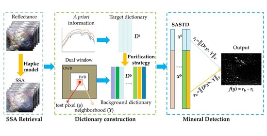
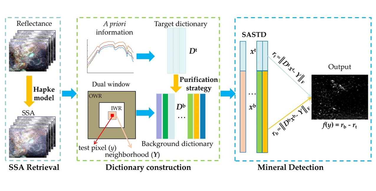
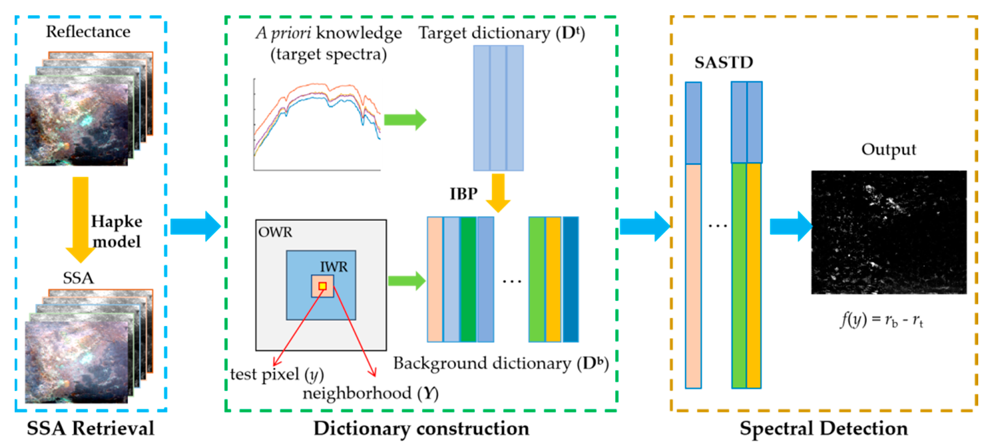
• Single-scattering albedo retrieval. The multiple scattering among mineral particles introduces nonlinearities in reflectance. The SSA is linearly additive in visible and near-infrared wavelengths [27]. The purpose of this step is to convert the reflectance to SSA. Consequently, the linear target detection method can be implemented on SSA data;
• Background and target dictionaries construction. The target dictionary D^t is constructed using a priori knowledge of target spectra, while the background dictionary D^b is generated locally through a dual window. However, target pixels may fall into D^b due to improper window size settings relative to mineral distribution size or the sliding window process. We propose an iterative background purification method to remove the potential target pixels in D^b.
• Spectral reconstruction and target detection. A spatially adaptive sparse representation for target detection (SASTD) is adopted in this work, which incorporates spatial information into target detection. The final detection is in favor of the class that has the lowest reconstruction error.

3.2.1. Single-Scattering Albedo Retrieval

SSA is the ratio of scattering efficiency to total extinction (scattering and absorption) efficiency. The Hapke bidirectional reflectance distribution function enables us to convert the reflectance to the SSA. The function is described as follows [26]

$$r(i,e,g)=\frac{\omega }{4}\frac{{\mu }_0}{({\mu }_0+\mu )}[(1+B(g))P(g)+H({\mu }_0)H(\mu )-1]$$

(5)

where r(i,e,g) is the radiance factor; i, e, and g are incidence, emergence, and phase angles, respectively; μ₀ and μ are the cosines of the incidence angle and emergence angle; ω is the average single-particle scattering albedo; B(g) is the backscattering function describing the opposition effect which is strong at a near-zero phase angle; P(g) is the surface phase function describing how reflected energy changes with the viewing direction; and H is the Chandrasekhar integral function associated with the observation geometry. The H function is approximated by [26]

$$H(\mu )=\frac{1+2\mu }{1+2\mu \gamma },\gamma =\sqrt{1-\omega }$$

(6)

We set P(g) = 1 with the assumption that particles scatter isotropically [40]. The opposition effect can be omitted when the phase angle is greater than 15° [40]. We assumed B(g) = 0 because the phase angles of the data used in this study are greater than 15°. Using Equations (5) and (6), we calculated reflectance at every SSA value from zero to one at a step size of 0.0001 [39]. Then a lookup table approach is used to retrieve the SSA from the observed HSI.

3.2.2. Iterative Background Dictionary Purification

The background dictionary D^b is generated locally for each pixel through a dual concentric window [21]. The dual-window is widely used to construct the background dictionary in representation theory-based methods [41]. As shown in Figure 5a, the yellow square denotes the pixel under test, whereas the red object represents targets. The local region of each test pixel is split into two parts: a small inner window region (IWR), which is centered within a broader outer window region (OWR). The IWR serves as a guard window to avoid the target signals leakage while the OWR is employed to model the local background characterization. Pixels in the annulus (the light gray region in Figure 2) are selected as background dictionary. In practice, there are three possible scenarios for the background dictionary: (1) as shown in Figure 5a, the ideal case is that the inner window is larger than the targets and no target pixels exist in the outer region. (2) In Figure 5b, although the inner window is larger than the size of targets, some targets fall into the annulus during the sliding process. (3) As shown in Figure 5c, the inner window is smaller than the targets. Thus, the targets impinge into the outer window. The last two cases generate an impure background dictionary, which consists of both background and target pixels. The target interference issue leads to inferior detection performance [25].

To obtain a relatively pure background D^b, we used the spectral angle technique [42] to remove doubtful target pixels in the dual window. The spectral angle distance (SAD) between ${\left\{D_{\mathrm{i}}^{\mathrm{b}}\right\}}_{i=1,2,\dots ,N_{\mathrm{b}}}$ and ${\left\{D_{\mathrm{j}}^{\mathrm{t}}\right\}}_{j=1,2,\dots ,N_{\mathrm{t}}}$ is defined by [42]

$$SAD(i,j)={\cos }^{-1}(\frac{dot(D_{\mathrm{i}}^{\mathrm{b}},D_{\mathrm{j}}^{\mathrm{t}})}{{\Vert D_{\mathrm{i}}^{\mathrm{b}}\Vert }_2\times {\Vert D_{\mathrm{j}}^{\mathrm{t}}\Vert }_2})$$

(7)

where dot( , ) denotes the inner product of two vectors; cos⁻¹ implements the inverse cosine operation. The smaller the spectral angle, the more similar the background signature to the target pixel. The background spectrum with a spectral angle smaller than a specified threshold is removed. If the number of remaining background pixels is less than a given number (we set the value as N^t since the number of target pixels in D^t is two orders of magnitude less than that of D^b), we enlarge the window size of IWR and OWR at a step size of 2 lines/columns. Then the dictionary purification is performed iteratively until the number of remaining background spectra is greater than N^t. With the IBP process, we mitigate the target interference and have flexible window size settings.

3.2.3. Spectral Reconstruction and Target Detection

In STD, the test pixel is treated individually regardless of the correlation between neighboring pixels [21]. However, the neighboring pixels often contain similar materials in real world. To incorporate the spatial pattern into target detection, we pay attention to the non-local spatial information [23]. Specifically, the spectral difference between the central pixel and its neighbors is used to determine the weight for each neighboring pixel. Assuming Y = [y₁, y₂, …y_m] is a matrix whose columns are pixels in a small neighborhood ${\mathcal{N}}_m$, The weight function is defined as

$$w=\phi (d(i,j))$$

(8)

where d( , ) is used to compare the spectral distance between two spatial patches

$$d(i,j)=\frac{1}{L}{\displaystyle {\sum }_{\mathrm{k}=1}^{\mathrm{L}}({\Vert P{(i)}_{\mathrm{k}}-P{(j)}_{\mathrm{k}}\Vert }_2)}$$

(9)

where pixels i and j belong to ${\mathcal{N}}_m$; P(i) and P(j) are matrixes whose columns are pixels surrounding i and j, respectively. The patch size is set as 7 × 7 as suggested in [23]; φ( ) is employed to convert the distance to weight, which is defined as

$$w=\phi (d(i,j))={(1-{(\frac{d(i,j)}{t})}^2)}^2$$

(10)

where $t$ is used to control the decay of weight. We set $t$ as the maximum spectral patch distance within ${\mathcal{N}}_m$ so as to normalize the weight within the range [0,1]. This formula guarantees that the greater the distance, the lower the assigned weight will be.

Once the weights are obtained, the method is formulated as follows

$$YW=D[x_1,x_2,\cdots x_{\mathrm{m}}]=DX$$

(11)

where W = diag(w₁, w₂, …w_m) is a diagonal weighting matrix; D is the union of background and target dictionary; X is a sparse coefficient matrix with a few nonzero rows, which can be recovered by solving the following problem

$$\min {\Vert YW-DX\Vert }_{\mathrm{F}} s.t.{\Vert X\Vert }_{\mathrm{row},0}\le K$$

(12)

where ${\Vert X\Vert }_{\mathrm{row},0}$ denotes the number of nonzero rows of X; K is the sparsity level. We used the simultaneous orthogonal matching pursuit (SOMP) algorithm [20] to solve the problem (12). The label of the test pixel is in favor of which class has the minimum reconstruction error

$$f(y)={\Vert YW-D^{\mathrm{b}}{X}^{\mathrm{b}}\Vert }_2-{\Vert YW-D^{\mathrm{t}}{X}^{\mathrm{t}}\Vert }_2$$

(13)

where X^b and X^t are the rows of the recovery matrix X corresponding to D^b and D^t, respectively.

3.3. Experimental Settings and Evaluation Metrics

For laboratory HSI, the proposed method is compared with the following detection algorithms: (1) constrained energy minimization (CEM) [35]; (2) matched filter (MF) [43]; (3) hierarchical CEM (hCEM) [44]; (4) STD [21]; (5) SASTD [23]. All the experiments are implemented using MATLAB 2017a on a desktop with 3.4-GHz CPU and 16-GB Memory. The detection performance is evaluated by two quantitative metrics: the Receiver Operating Characteristic (ROC) curve and Area Under ROC Curve (AUC) value. The ROC curve illustrates the relationship between the detection probability P_d and the false alarm rate P_f at a series of thresholds. The area under the ROC curve is called AUC value. P_d and P_f are defined by [44]

$$P_{\mathrm{d}}=\frac{N_{\det \mathrm{ected}}}{N_{\mathrm{T}}},P_{\mathrm{f}}=\frac{N_{\mathrm{mis}}}{N_{\mathrm{all}}}$$

(14)

where N_detected is the number of detected target pixels at a certain threshold; N_T denotes the number of total target pixels in the image; N_mis represents the number of background pixels mistaken as targets; N_all is the number of total pixels in the image.

We set the IWR as 15 × 15, which is the same as the sample size. The OWR was set as 21 × 21. Three pixels from the 100% serpentine tray were randomly chosen as the target spectra, thus N^t = 3. For all algorithms, we used the same target spectra as input. For CEM and hCEM, the mean of the three selected target pixels is used as the target signature. The optimal parameters of the sparsity level for STD were set according to the corresponding AUC values. For the proposed algorithm, the threshold of SAD (θ) between the spectrum in the target dictionary and the spectrum in the background dictionary is set as 1°, the sparsity level K is set as 10, the neighbor size is set as 5 × 5. The detailed parameter analysis of our method is given in Section 4.1.2.

For CRISM data, we used a set of conservative parameter values according to the parameters analyzed in Section 4.1.2. The size of the neighborhood, IWR, and OWR are set as 3 × 3, 23 × 23 and 31 × 31, respectively. The threshold of SAD is set as 2°. The sparsity level is set as 20. We randomly select three serpentine pixels in each image according to the identification results by [37]. The selected target spectra are exhibited in Figure 3c,d, respectively.

4. Experimental Results

In this section, the superiority of the proposed method was first evaluated on a laboratory HSI. We compared HSASTD-IBP with several traditional and state-of-the-art target detection algorithms. The performance was assessed by three aspects, including detection map, ROC curve, and AUC value. Due to parameter settings that could affect the detection result, we further investigated the effects of parameter settings. Then the proposed algorithm was applied to two well-studied CRISM data sets.

4.1. Experiments with Laboratory Data

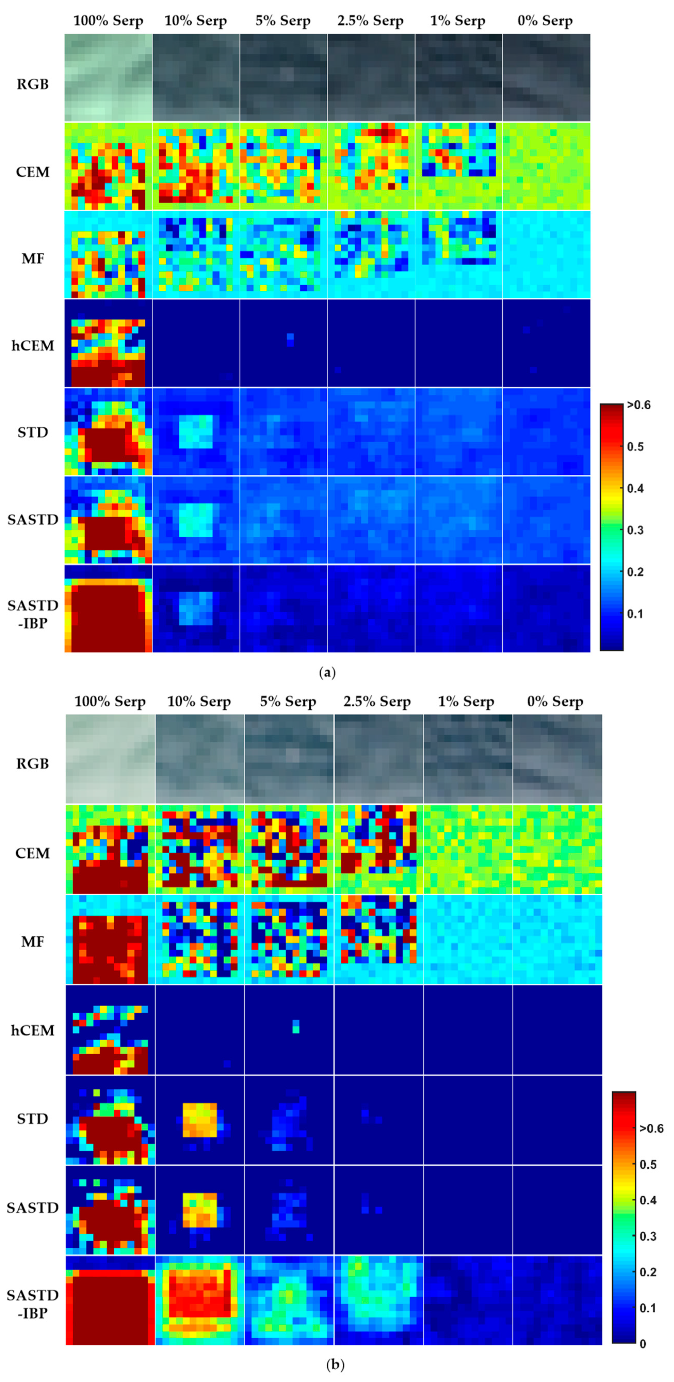
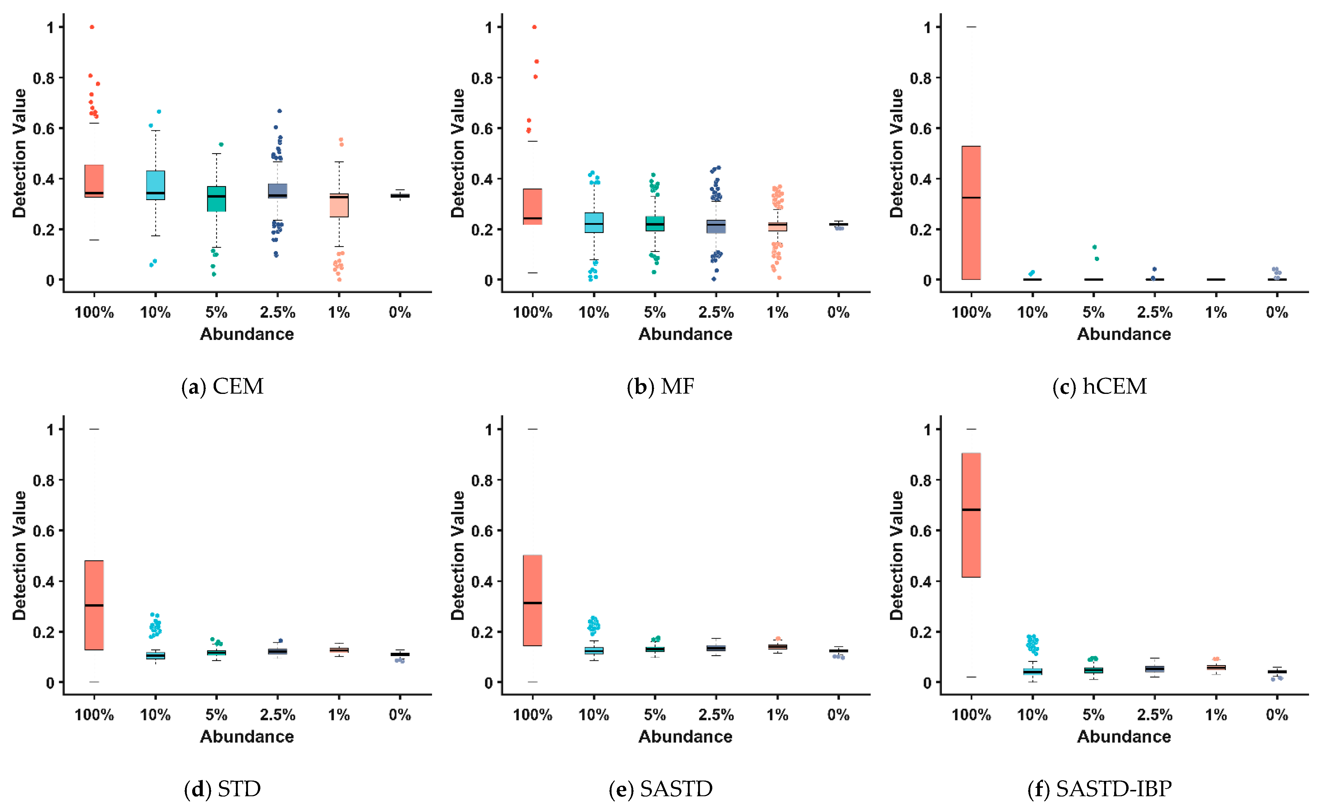
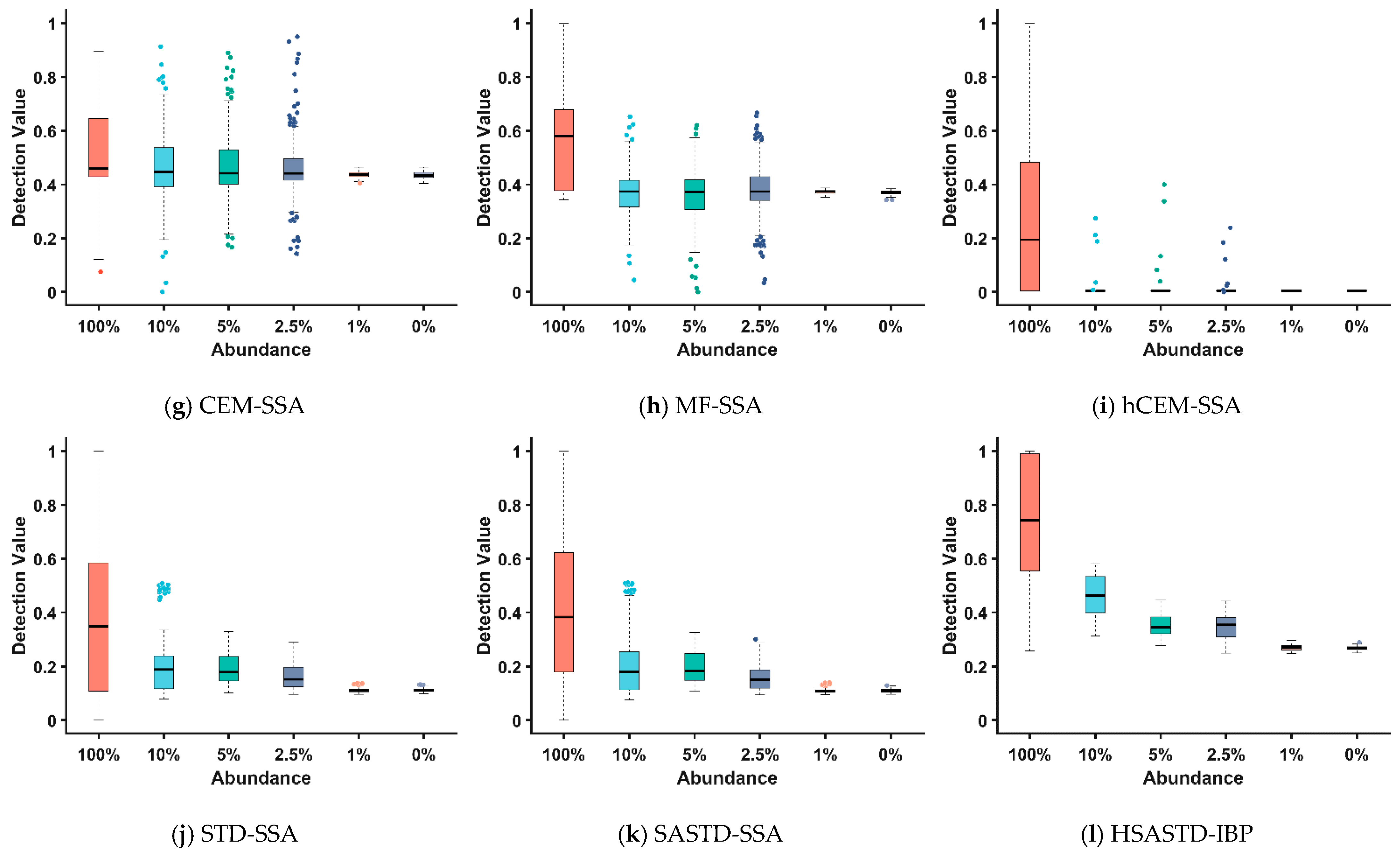
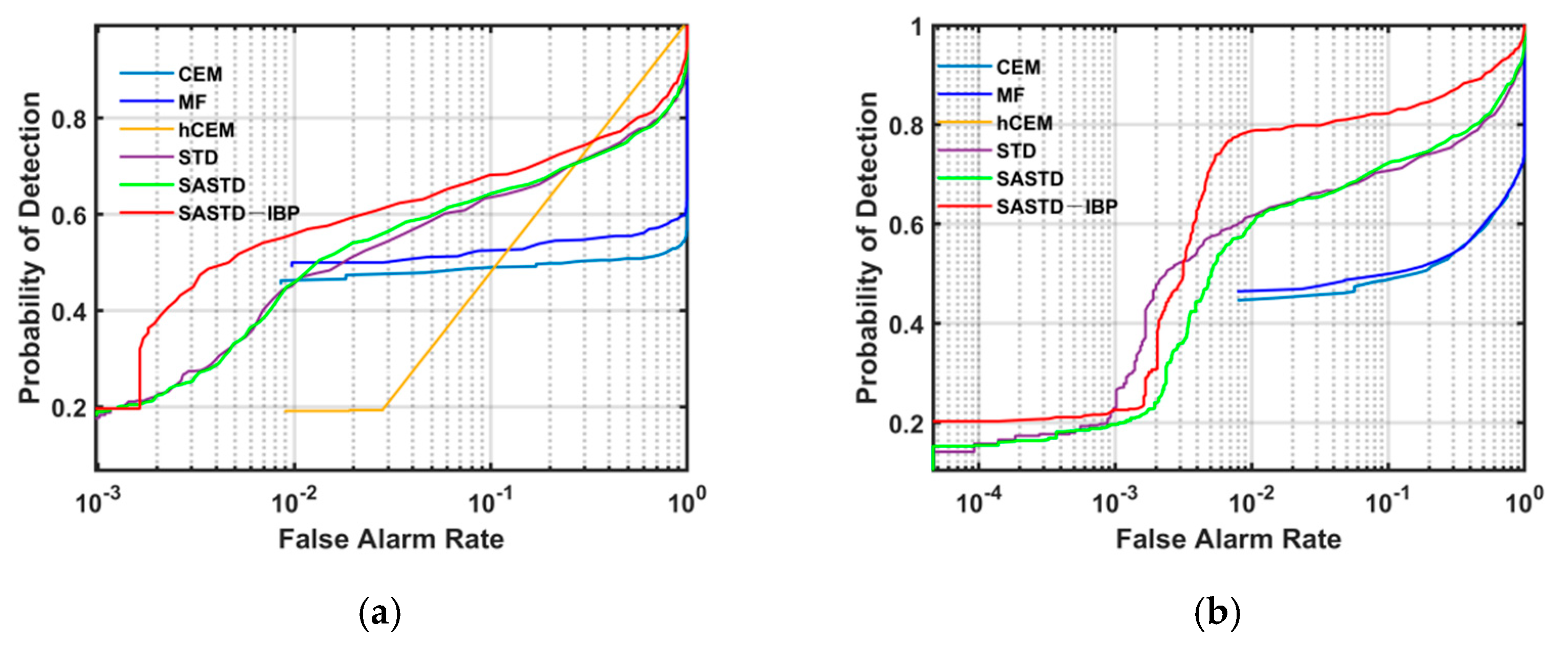
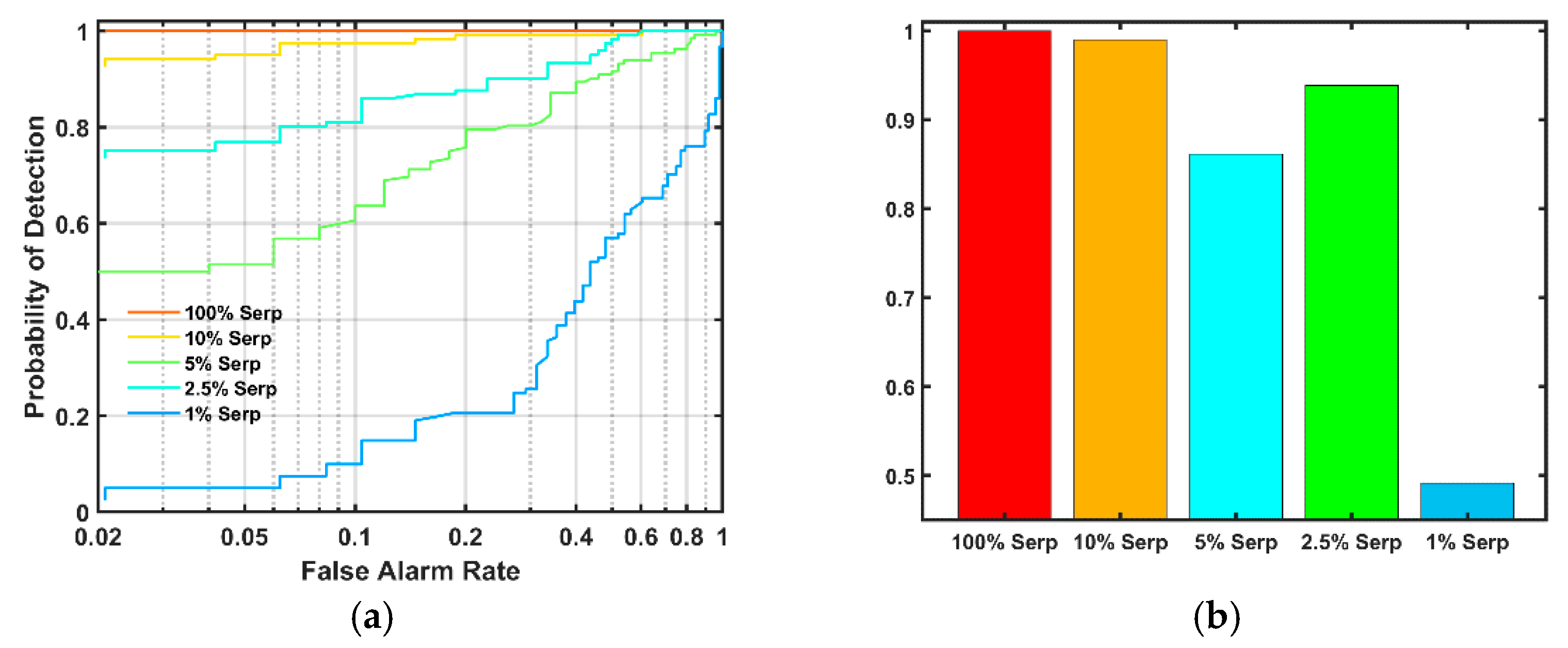
4.1.1. Detection Performance

The two-dimensional detection maps of all methods on reflectance and SSA data are displayed in Figure 6a,b, respectively. The first row in each panel is the false-color image (R: 2.32 μm, G: 2.12 μm, B: 1.39 um), displaying the variations of samples’ surfaces. The subsequent rows are detection maps derived from different target detection methods. The serpentine abundance decreases from left to right. For a fair comparison, the detection values are normalized to [0, 1] for the output of each method. The reddish color represents that the pixel is more likely to be a serpentine, while the blueish color indicates that the pixel belongs to MGS-1.

As shown in Figure 6a, CEM and MF detect parts of pure serpentine and serpentine mixtures, while hCEM mainly identifies pixels in the 100% serpentine. The 100% serpentine pixels in the hCEM map are more distinguishable than those in CEM and MF maps. The reason is that hCEM relies on a hierarchical layer-by-layer filtering procedure. Thus, weak targets might be suppressed. All the sparse representation-based detection algorithms detect 100% and 10% serpentine. However, STD and SASTD only detect parts of 100% serpentine pixels. That is because the target interference degrades the discrimination ability. As shown in Figure 6b, the detection performances are boosted on SSA data. The detection values of 100% serpentine pixels in CEM and MF are higher than those in Figure 6a. The proposed approach gets high detection values for the 100% and 10% serpentine pixels as well as STD, SASTD. Additionally, our method detects almost all 5% and 2.5% serpentine mixtures when compared with the SASTD detection maps, demonstrating that dictionary purification mitigates the target interference efficiently. Overall, the SSA versions of these detection algorithms outperform their reflectance versions. However, the 1% serpentine mixture is below the detection limit of our method. That is because the 1% serpentine spectral features are highly similar to the pure MGS-1.

The statistics of detection values for different algorithms were illustrated in Figure 7. On each box, the central black line indicates the median. The bottom and top edges of the box indicate the 25th and 75th percentiles, respectively. The outlier is plotted individually using the solid circle. For each panel, the detection values decline from left to right as the serpentine abundance decreases from 100% to 0%. The first two rows (Figure 7a–f) show the boxplots of each detector on the original reflectance data. As shown in Figure 7a,b, CEM and MF cannot effectively discriminate the various serpentine mixtures since the median of each box overlaps. As for the last four detectors (Figure 7c–f), the detection value of 100% serpentine is significantly greater than the low abundance mixtures. For hCEM, the signals of mixtures are strongly suppressed, thus, their boxes are extremely flat. For the representation theory-based detectors, although the median of low abundance serpentine mixtures is slightly above that of MGS-1, it is still difficult to discriminate them. The last two rows (Figure 7g–l) show the boxplots of each detector on the single-scattering albedo data. Generally, the same trends can be found for the first three statistic-based detectors. As shown in Figure 7g–i, the detection values of the 1% serpentine and MGS-1 boxes overlap with those of the other mixtures’ boxes. Thus, it is hard to completely separate these different serpentine mixtures apart by a threshold. For the representation theory-based detectors, the 2.5%, 5%, and 10% serpentine boxes are elevated when compared with their reflectance counterparts. The detection value gaps among different serpentine samples are clear in Figure 7l. The medians of mixtures (abundance > 2.5%) are significantly different from those of 1% and 0% mixtures. More explicitly, the serpentine detection limit of our algorithm is 2.5%.

Conventionally, a better TD algorithm gets higher P_d at the same P_f. As shown in Figure 8a, for the laboratory reflectance data, the ROC curves of sparse representation-based detection algorithms are above those of traditional detectors CEM, hCEM, and MF. Moreover, the ROC curve of SASTD-IBP encloses those of the other detectors, demonstrating that dictionary purification process improves the detection accuracy. A similar phenomenon is found in Figure 8b. For the SSA data, the ROC curve of the proposed method broadly encloses those of other detectors, especially when P_f ranges from 0.005 to 1. It is also observed that the ROC curve of each detection algorithm for the reflectance data is below that of its SSA version, which makes clear that SSA domain is more suitable for mineral detection.

The AUC values and computation times for the different detectors are shown in

Table 2. AUC values and running time (seconds) for the different detection algorithms. The best results are emphasized in bold.

	Dataset	Reflectance		SSA
Algorithm		AUC	Time	AUC	Time
CEM		0.5090	0.19	0.5924	0.20
MF		0.5584	0.32	0.5971	0.41
hCEM		0.5848	1.86	0.5998	1.93
STD		0.7455	130.78	0.8025	139.27
SASTD		0.7469	161.62	0.8121	160.28
SASTD-IBP		0.7799	179.34	0.8965	181.79

. The best results are emphasized in bold. In reflectance data, the AUC value obtained by SASTD is improved from 0.7469 to 0.7799 by purifying the background dictionary. In SSA data, the HSASTD-IBP achieves the best AUC value of 0.8965. The relative increment of each method on the SSA dataset ($\frac{AU{C}_{\mathrm{SSA}}-AU{C}_{\mathrm{reflec}\tan \mathrm{ce}}}{AU{C}_{\mathrm{reflec}\tan \mathrm{ce}}}$) is 16.39%, 6.93%, 2.56%, 7.65%, 8.73%, and 14.95%, respectively. In terms of computation time, the traditional method (e.g., CEM, MF, hCEM) takes about 1 s to run the algorithm. For the sparse representation-based method, it takes more than 100 s, which is two orders of magnitude of running time for the statistic-based method. However, this computation burden is acceptable considering its superior performance.

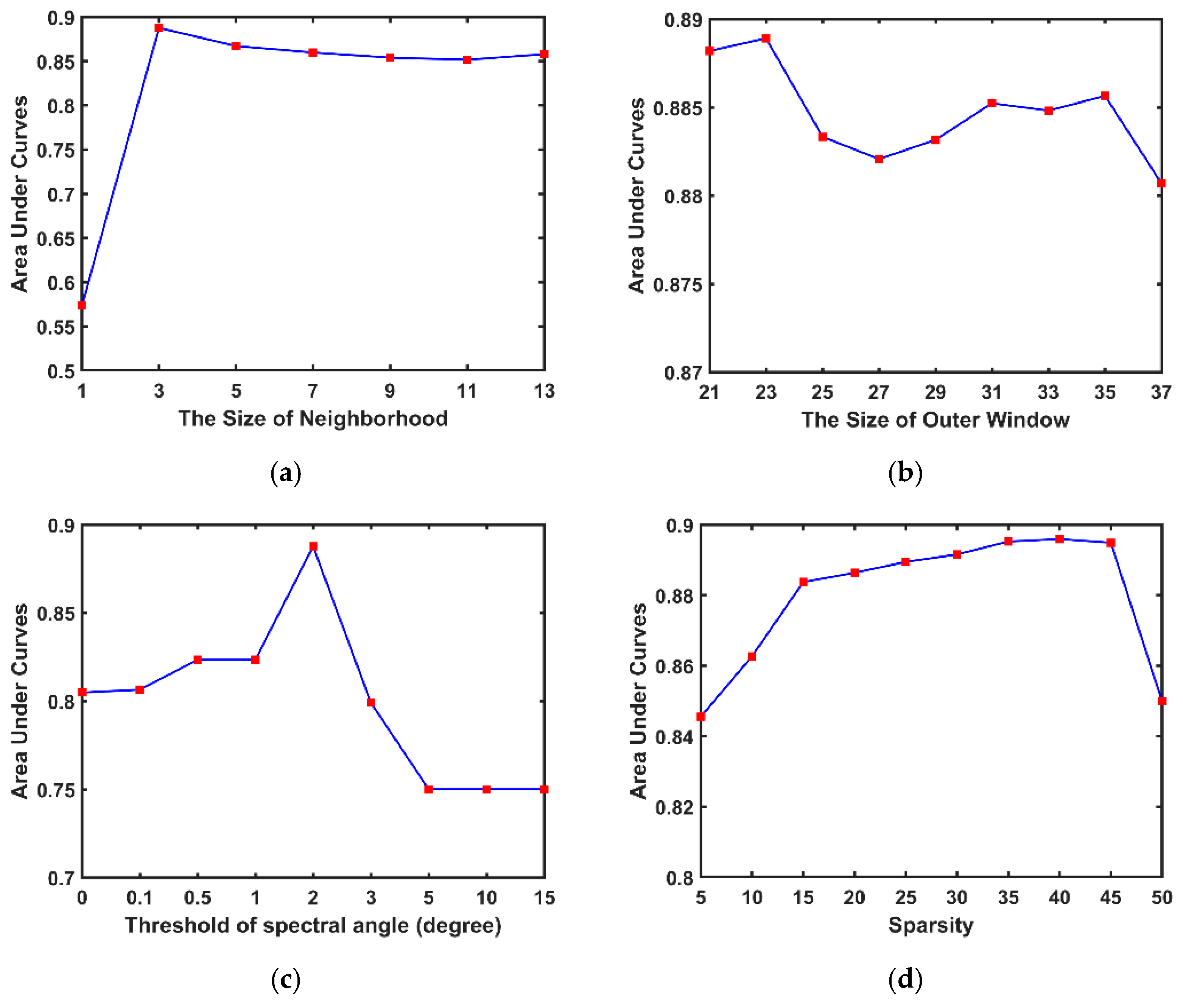
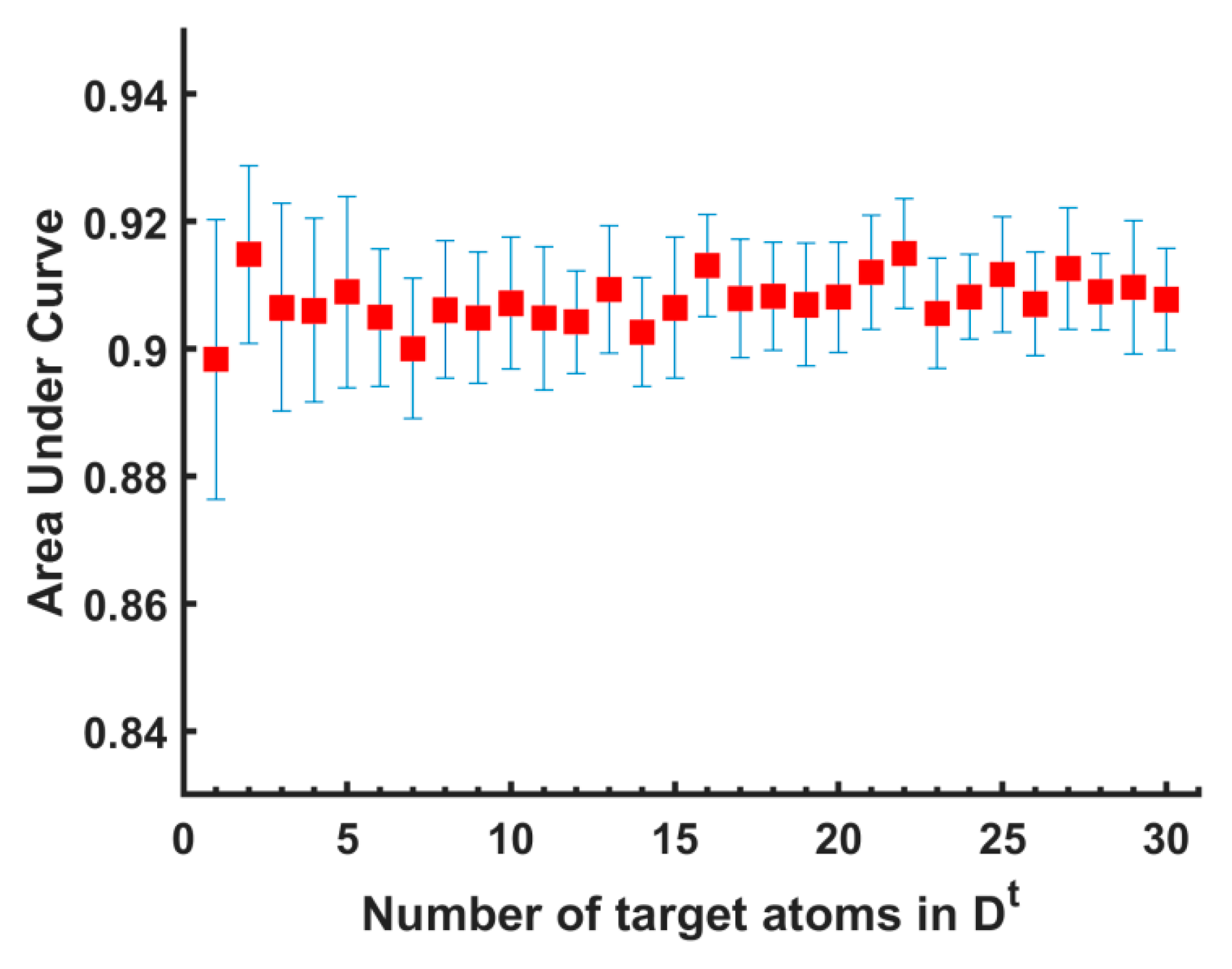
4.1.2. Parameter Analysis

The laboratory SSA data is used to investigate the effects of various parameters on detection performance. There are four parameters in HSASTD-IBP, namely the neighborhood size centering at the test pixel, the dual window sizes, the SAD threshold θ, and the sparsity level K. Each time we focus on one specific parameter and keep the others fixed. For the neighborhood size, we use a 1 × 1, 3 × 3, 5 × 5, 7 × 7, 9 × 9, 11 × 11, and 13 × 13 window neighborhoods. The size of the IWR is fixed as above mentioned 15, and the range of the OWR size is set to [21, 23, 25, 27, 29, 31, 33, 35, 37]. The range of θ is set as [0, 0.1, 0.5, 1, 2, 3, 5, 10, 15] degree, and the range of K is set to [5, 10, 15, 20, 25, 30, 35, 40, 45, 50]. Detection performance is evaluated by the AUC value.

We first analyzed the performance of the HSASTD-IBP under the varying size of the neighborhood. As shown in Figure 9a, the AUC value improves rapidly from 1 to 3, which proves that spatial correlation boosts detection accuracy. However, a broader neighborhood may contain pixels different from the central pixel. Thus, the AUC value tends to generally decreases. The effect of outer window size on serpentine detection was further evaluated. As shown in Figure 9b, the AUC value increases at first and then slightly fluctuates as the increment of OWR. Figure 9c exhibits the sensitiveness of the performance on θ. The AUC value climbs as the increase of threshold and reaches a peak of 0.8877 at θ = 2°. The improvement benefits from those potential target pixels in the background dictionary are removed. Then a sudden decline is observed when θ exceeds 2°. Finally, we illustrate how the detection results are affected by the sparsity level K in Figure 9d. The sparsity level K refers to the number of nonzero rows in $X$. The AUC value gradually rises as the increase of K and achieves the maximum value 0.8959 at K = 40, then rapidly decreases.

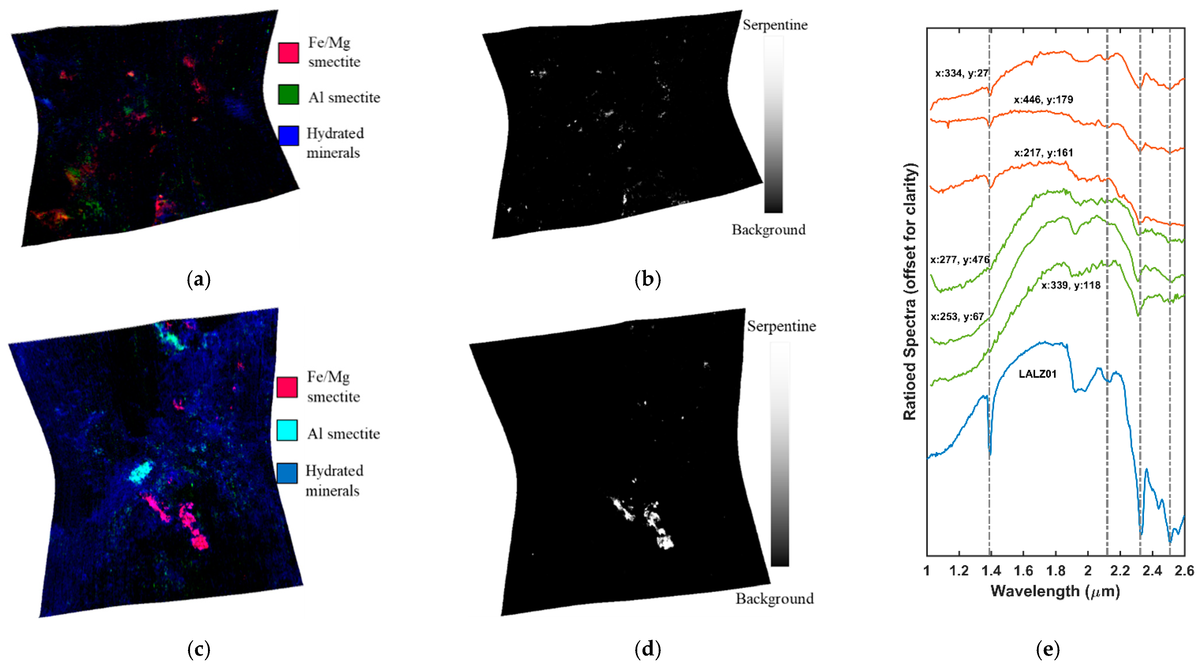
4.2. Application on CRISM Data

Due to no groundtruth for the two images, a false-color map indicating the spatial distribution of minerals is created by assigning RGB values to the intensities of phyllosilicates related indexes. The meaning and formula of each index are illustrated in Table 1. Image stretching is performed on each index individually (lower bound: 0.005, upper bound: 99.9% of the cumulative histogram). The purpose of stretching is to ensure positive values of absorption depth while omitting outliers. As shown in Figure 10a,c, red/magenta colors indicate the presence of Fe/Mg smectites, while green/cyan colors indicate the presence of Al/Si-OH bearing minerals. The final detection maps were also stretched and shown in Figure 10b,d. The serpentine detection results are consistent with the spatial distribution of red/magenta colors in the index maps. In addition, the ratioed spectra of high detection value regions are used for spectral validation. As shown in Figure 10e, the orange spectra are extracted from FRT0000634B while the green spectra are acquired from FRT0000ABCB. Each curve is the ratio of an average of 5 × 5 spectra of the central pixel to the average of neutral pixels in the same columns. The low signal to noise of orbital data often obscures the narrow absorption, thus, the weak 1.39 μm absorption in ratioed spectra is shallow or absent. Nonetheless, these ratioed spectra have the same absorption features at 2.12, 2.32, 2.5 μm as the laboratory serpentine spectrum LALZ01 (http://speclib.rsl.wustl.edu/), which further corroborates our detection results. It is worth noting that the spectral index does not represent a specific mineral distribution. Thus, a quantitative comparison is infeasible.

5. Discussion

In this section, the detection limit of serpentine abundance is first assessed, which helps to answer the question of how much confidence we have about our detection result. After that, the impact of prior information (target spectra) on detection performance is discussed.

Detection limit: To explore the minimum detectable abundance of serpentine, we analyze the performance of the proposed method on each sample tray. Figure 11a exhibits the ROC curves of each serpentine tray. The detection probabilities (P_d) is a function of serpentine abundance. As the serpentine abundance decreases, the detection performance declines. For example, as shown in Figure 11a, when P_f = 0.05, P_d for the 5 trays are 100%, 80.99%, 74.38%, 69.70%, and 3.31%, respectively. As displayed in Figure 11b, the AUC value for each tray gradually drops as the serpentine abundance decreases. An abrupt decay is observed for the 1% serpentine tray. The trend is expected since the lower the abundance of serpentine the less spectral similarity to the target. The stripe noise and powder inhomogeneous within 5% serpentine impair the performance. Thus, the AUC value of 5% serpentine is smaller than that of 2.5% serpentine. It should be noted that the detection limit is based on the laboratory binary mixture data. In practice, the martian surface is more complicated. Moreover, the pervasive martian dust potentially masks the mineralogical signatures, which further hinders the mineral detection.

Impact of prior information: Due to intrinsic (e.g., grain size) and extrinsic (e.g., imaging condition) factors, targets could show spectral variability. The effect of the selected target spectra on detection is evaluated here. The number of target spectra N^t is set from 1 to 30. Each time we randomly select N^t pixels from 100% serpentine tray as input and repeated 20 times. The mean (red square) and standard deviation (blue bar) of AUC values are shown in Figure 12. The AUC value slightly increases at first and then tends to saturate. The variation at each point shows the detection uncertainty because of spectral variability. Figure 12 shows that the proposed method achieves a satisfactory performance with a small number of target spectra.

For practical applications, there are two solutions to acquire prior target information. One approach is to extract the in-scene target signatures by endmember extraction. This approach has been proved beneficial to detection performance [45]. However, endmember extraction algorithms tend not to work well when there are few targets in the image. An alternative approach is to explore the available spectral library. For example, the target mineral’s reflectance and band depth tend to vary as the grain size changes. The spectral library usually has multiple target spectra, which sufficiently represents the spectral variability. This approach sidesteps extracting target spectra from the image, which promotes the application to large volume of data. Although there are discrepancies between spectral library and image due to imaging conditions, calibration procedures, and spatial resolutions, it is still promising to employ a spectral library to construct a target dictionary if these mismatches are well addressed.

6. Conclusions

In this study, a new mineral detection method was proposed by joining the Hapke radiative transfer model and SASTD with iterative background purification. Laboratory mineral mixtures and two well-studied CRISM images with serpentine were used to validate our method. Several interesting conclusions can be drawn: (1) The proposed method achieves the best detection performance in both reflectance and SSA data. (2) Our method is able to detect low abundance serpentine (above 2.5%) in the laboratory binary mixtures. The 1% serpentine is below the detection limit since the signal is too weak. (3) The detection performance is boosted by purifying the background dictionary. The IBP strategy proposed in this work can be implanted into other representation theory-based detection methods. (4) The SSA versions of these detectors are superior to their reflectance versions, demonstrating that SSA has excellent potential for discriminating target minerals from background minerals.

Overall, the proposed method enables the search for subpixel-level, less exposed, but scientifically valuable deposits. The laboratory imaging offers a critical link in scale between field measurements and orbital observations. Acquiring new HSIs containing other hydrated minerals (e.g., nontronite, selenite, calcite, kaolinite) and MGS-1 mixtures to tailor the proposed method will be the focus of our future research. Additionally, we also plan to study the effect of grain size on detection result in the future.

References

1. Plaza, A.; Benediktsson, J.A.; Boardman, J.W.; Brazile, J.; Bruzzone, L.; Camps-Valls, G.; Chanussot, J.; Fauvel, M.; Gamba, P.; Gualtieri, A. Recent advances in techniques for hyperspectral image processing. Remote Sens. Environ. 2009, 113, S110–S122. [Google Scholar] [CrossRef]
2. Bibring, J.P.; Langevin, Y.; Gendrin, A.; Gondet, B.; Poulet, F.; Berthé, M.; Soufflot, A.; Arvidson, R.; Mangold, N.; Mustard, J. Mars surface diversity as revealed by the OMEGA/Mars Express observations. Science 2005, 307, 1576–1581. [Google Scholar] [CrossRef] [PubMed] [Green Version]
3. Murchie, S.; Arvidson, R.; Bedini, P.; Beisser, K.; Bibring, J.P.; Bishop, J.; Boldt, J.; Cavender, P.; Choo, T.; Clancy, R.T. Compact Reconnaissance Imaging Spectrometer for Mars (CRISM) on Mars Reconnaissance Orbiter (MRO). J. Geophys. Res. Atmos. 2007, 112, 431–433. [Google Scholar] [CrossRef]
4. Ehlmann, B.L.; Edwards, C.S. Mineralogy of the Martian Surface. Earth Planet. Sci. 2014, 42, 291–315. [Google Scholar] [CrossRef] [Green Version]
5. Murchie, S.L.; Mustard, J.F.; Ehlmann, B.L.; Milliken, R.E.; Bishop, J.L.; Mckeown, N.K.; Dobrea, E.Z.N.; Seelos, F.P.; Buczkowski, D.L.; Wiseman, S.M. A synthesis of Martian aqueous mineralogy after 1 Mars year of observations from the Mars Reconnaissance Orbiter. J. Geophys. Res. Planets 2009, 114, E00D06. [Google Scholar] [CrossRef]
6. Carter, J.; Poulet, F.; Bibring, J.P.; Mangold, N.; Murchie, S. Hydrous minerals on Mars as seen by the CRISM and OMEGA imaging spectrometers: Updated global view. J. Geophys. Res. Atmos. 2013, 118, 831–858. [Google Scholar] [CrossRef]
7. Mustard, J.F.; Murchie, S.L.; Pelkey, S.M.; Ehlmann, B.L.; Milliken, R.E.; Grant, J.A.; Bibring, J.P.; Poulet, F.; Bishop, J.; Dobrea, E.N. Hydrated silicate minerals on Mars observed by the Mars Reconnaissance Orbiter CRISM instrument. Nature 2008, 454, 305–309. [Google Scholar] [CrossRef]
8. Ehlmann, B.L.; Mustard, J.F.; Swayze, G.A.; Clark, R.N.; Bishop, J.L.; Poulet, F.; Des Marais, D.J.; Roach, L.H.; Milliken, R.E.; Wray, J.J.; et al. Identification of hydrated silicate minerals on Mars using MRO-CRISM: Geologic context near Nili Fossae and implications for aqueous alteration. J. Geophys. Res. 2009, 114, 538–549. [Google Scholar] [CrossRef]
9. Liu, Y.; Glotch, T.D.; Scudder, N.A.; Kraner, M.L.; Condus, T.; Arvidson, R.E.; Guinness, E.A.; Wolff, M.J.; Smith, M.D. End-member Identification and Spectral Mixture Analysis of CRISM Hyperspectral Data: A Case Study on Southwest Melas Chasma, Mars. J. Geophys. Res. Planets 2016, 121, 2004–2036. [Google Scholar] [CrossRef]
10. Lin, H.; Zhang, X. Retrieving the hydrous minerals on Mars by sparse unmixing and the Hapke model using MRO/CRISM data. Icarus 2017, 288, 160–171. [Google Scholar] [CrossRef]
11. Wray, J.J.; Murchie, S.L.; Bishop, J.L.; Ehlmann, B.L.; Milliken, R.E.; Wilhelm, M.B.; Seelos, K.D.; Chojnacki, M. Orbital evidence for more widespread carbonate-bearing rocks on Mars. J. Geophys. Res. Planets 2016, 121, 652–677. [Google Scholar] [CrossRef] [Green Version]
12. Sun, V.Z.; Milliken, R.E. Ancient and recent clay formation on Mars as revealed from a global survey of hydrous minerals in crater central peaks. J. Geophys. Res. Planets 2015, 120, 2293–2332. [Google Scholar] [CrossRef]
13. Pelkey, S.M.; Mustard, J.F.; Murchie, S.; Clancy, R.T.; Wolff, M.; Smith, M.; Milliken, R.; Bibring, J.P.; Gendrin, A.; Poulet, F.; et al. CRISM multispectral summary products: Parameterizing mineral diversity on Mars from reflectance. J. Geophys. Res. 2007, 112, 1–18. [Google Scholar] [CrossRef]
14. Viviano-Beck, C.E.; Seelos, F.P.; Murchie, S.L.; Kahn, E.G.; Seelos, K.D.; Taylor, H.W.; Taylor, K.; Ehlmann, B.L.; Wiseman, S.M.; Mustard, J.F.; et al. Revised CRISM spectral parameters and summary products based on the currently detected mineral diversity on Mars. J. Geophys. Res. Planets 2014, 119, 1403–1431. [Google Scholar] [CrossRef] [Green Version]
15. Bioucas-Dias, J.M.; Plaza, A.; Dobigeon, N.; Parente, M.; Du, Q.; Gader, P.; Chanussot, J. Hyperspectral Unmixing Overview: Geometrical, Statistical, and Sparse Regression-Based Approaches. IEEE J. Sel. Top. Appl. Earth Obs. Remote Sens. 2012, 5, 354–379. [Google Scholar] [CrossRef] [Green Version]
16. Poulet, F.; Carter, J.; Bishop, J.L.; Loizeau, D.; Murchie, S.M. Mineral abundances at the final four curiosity study sites and implications for their formation. Icarus 2014, 231, 65–76. [Google Scholar] [CrossRef]
17. Lin, H.; Mustard, J.F.; Zhang, X. A methodology for quantitative analysis of hydrated minerals on Mars with large endmember library using CRISM near-infrared data. Planet. Space Sci. 2019, 165, 124–136. [Google Scholar] [CrossRef]
18. Manolakis, D.; Truslow, E.; Pieper, M.; Cooley, T. Detection Algorithms in Hyperspectral Imaging Systems: An Overview of Practical Algorithms. IEEE Signal Process. Mag. 2014, 31, 24–33. [Google Scholar] [CrossRef]
19. Nasrabadi, N.M. Hyperspectral Target Detection: An Overview of Current and Future Challenges. IEEE Signal Process. Mag. 2014, 31, 34–44. [Google Scholar] [CrossRef]
20. Chen, Y.; Nasrabadi, N.M.; Tran, T.D. Simultaneous Joint Sparsity Model for Target Detection in Hyperspectral Imagery. IEEE Geosci. Remote Sens. Lett. 2011, 8, 676–680. [Google Scholar] [CrossRef]
21. Chen, Y.; Nasrabadi, N.M.; Tran, T.D. Sparse Representation for Target Detection in Hyperspectral Imagery. IEEE J. Sel. Top. Signal Process. 2011, 5, 629–640. [Google Scholar] [CrossRef]
22. Zhang, Y.; Du, B.; Zhang, L. A Sparse Representation-Based Binary Hypothesis Model for Target Detection in Hyperspectral Images. IEEE Trans. Geosci. Remote Sens. 2015, 53, 1346–1354. [Google Scholar] [CrossRef]
23. Zhang, Y.; Du, B.; Zhang, Y.; Zhang, L. Spatially Adaptive Sparse Representation for Target Detection in Hyperspectral Images. IEEE Geosci. Remote Sens. Lett. 2017, 14, 1923–1927. [Google Scholar] [CrossRef]
24. Heylen, R.; Parente, M.; Gader, P. A review of nonlinear hyperspectral unmixing methods. IEEE J. Sel. Top. Appl. Earth Obs. Remote Sens. 2014, 7, 1844–1868. [Google Scholar] [CrossRef]
25. Wu, X.; Zhang, X.; Cen, Y. Multi-task Joint Sparse and Low-rank Representation Target Detection for Hyperspectral Image. IEEE Geosci. Remote Sens. Lett. 2019, 16, 1756–1760. [Google Scholar] [CrossRef]
26. Hapke, B. Theory of Reflectance and Emittance Spectroscopy; Cambridge University Press: Cambridge, UK, 1993. [Google Scholar]
27. Hapke, B. Bidirectional reflectance spectroscopy: 1. Theory. J. Geophys. Res. Solid Earth 1981, 86, 3039–3054. [Google Scholar] [CrossRef]
28. Cannon, K.M.; Britt, D.T.; Smith, T.M.; Fritsche, R.F.; Batcheldor, D. Mars global simulant MGS-1: A Rocknest-based open standard for basaltic martian regolith simulants. Icarus 2019, 317, 470–478. [Google Scholar] [CrossRef] [Green Version]
29. Allender, E.; Stepinski, T.F. Automatic, exploratory mineralogical mapping of CRISM imagery using summary product signatures. Icarus 2017, 281, 151–161. [Google Scholar] [CrossRef]
30. Van Ruitenbeek, F.J.A.; Bakker, W.H.; van der Werff, H.M.A.; Zegers, T.E.; Oosthoek, J.H.P.; Omer, Z.A.; Marsh, S.H.; van der Meer, F.D. Mapping the wavelength position of deepest absorption features to explore mineral diversity in hyperspectral images. Planet. Space Sci. 2014, 101, 108–117. [Google Scholar] [CrossRef]
31. Carter, J.; Poulet, F.; Murchie, S.; Bibring, J.P. Automated processing of planetary hyperspectral datasets for the extraction of weak mineral signatures and applications to CRISM observations of hydrated silicates on Mars. Planet. Space Sci. 2013, 76, 53–67. [Google Scholar] [CrossRef]
32. Combe, J.P.; Mouélic, S.L.; Sotin, C.; Gendrin, A.; Mustard, J.F.; Deit, L.L.; Launeau, P.; Bibring, J.P.; Gondet, B.; Langevin, Y. Analysis of OMEGA/Mars Express data hyperspectral data using a Multiple-Endmember Linear Spectral Unmixing Model (MELSUM): Methodology and first results. Planet. Space Sci. 2008, 56, 951–975. [Google Scholar] [CrossRef]
33. Gilmore, M.S.; Thompson, D.R.; Anderson, L.J.; Karamzadeh, N.; Mandrake, L.; Castaño, R. Superpixel segmentation for analysis of hyperspectral data sets, with application to Compact Reconnaissance Imaging Spectrometer for Mars data, Moon Mineralogy Mapper data, and Ariadnes Chaos, Mars. J. Geophys. Res. Planets 2011, 116, E07001. [Google Scholar] [CrossRef]
34. Schmidt, F.; Bourguignon, S.; Mouelic, S.L.; Dobigeon, N. Accuracy and Performance of Linear Unmixing Techniques for Detecting Minerals on OMEGA/Mars Express. In Proceedings of the Workshop on Hyperspectral Image & Signal Processing: Evolution in Remote Sensing, Lisbon, Portugal, 6–9 June 2011; pp. 1–4. [Google Scholar]
35. Farrand, W.H.; Harsanyi, J.C. Mapping the distribution of mine tailings in the Coeur d’Alene River Valley, Idaho, through the use of a constrained energy minimization technique. Remote Sens. Environ. 1997, 59, 64–76. [Google Scholar] [CrossRef]
36. Ehlmann, B.L.; Mustard, J.F.; Murchie, S.L. Geologic setting of serpentine deposits on Mars. Geophys. Res. Lett. 2010, 37, 53–67. [Google Scholar] [CrossRef] [Green Version]
37. Leask, E.K.; Ehlmann, B.L.; Dundar, M.M.; Murchie, S.L.; Seelos, F.P. Challenges in the Search for Perchlorate and Other Hydrated Minerals With 2.1-mu m Absorptions on Mars. Geophys. Res. Lett. 2018, 45, 12180–12189. [Google Scholar] [CrossRef] [PubMed] [Green Version]
38. McGuire, P.C.; Bishop, J.L.; Brown, A.J.; Fraeman, A.A.; Marzo, G.A.; Frank Morgan, M.; Murchie, S.L.; Mustard, J.F.; Parente, M.; Pelkey, S.M.; et al. An improvement to the volcano-scan algorithm for atmospheric correction of CRISM and OMEGA spectral data. Planet. Space Sci. 2009, 57, 809–815. [Google Scholar] [CrossRef] [Green Version]
39. Goudge, T.A.; Mustard, J.F.; Head, J.W.; Salvatore, M.R.; Wiseman, S.M. Integrating CRISM and TES hyperspectral data to characterize a halloysite-bearing deposit in Kashira crater, Mars. Icarus 2015, 250, 165–187. [Google Scholar] [CrossRef]
40. Mustard, J.F.; Pieters, C.M. Photometric phase functions of common geologic minerals and applications to quantitative analysis of mineral mixture reflectance spectra. J. Geophys. Res. Solid Earth 1989, 94, 13619–13634. [Google Scholar] [CrossRef]
41. Matteoli, S.; Diani, M.; Theiler, J. An Overview of Background Modeling for Detection of Targets and Anomalies in Hyperspectral Remotely Sensed Imagery. IEEE J. Sel. Top. Appl. Earth Obs. Remote Sens. 2014, 7, 2317–2336. [Google Scholar] [CrossRef]
42. Kruse, F.A.; Lefkoff, A.B.; Boardman, J.W.; Heidebrecht, K.B.; Shapiro, A.T.; Barloon, P.J.; Goetz, A.F.H. The spectral image processing system (SIPS)—interactive visualization and analysis of imaging spectrometer data. Remote Sens. Environ. 1993, 44, 145–163. [Google Scholar] [CrossRef]
43. Manolakis, D.; Shaw, G. Detection algorithms for hyperspectral imaging applications. IEEE Signal Process. Mag. 2002, 19, 29–43. [Google Scholar] [CrossRef]
44. Zou, Z.; Shi, Z. Hierarchical Suppression Method for Hyperspectral Target Detection. IEEE Trans. Geosci. Remote Sens. 2016, 54, 330–342. [Google Scholar] [CrossRef]
45. Shi, Y.; Lei, J.; Yin, Y.; Cao, K.; Li, Y.; Chang, C.-I. Discriminative feature learning with distance constrained stacked sparse autoencoder for hyperspectral target detection. IEEE Geosci. Remote Sens. Lett. 2019, 16, 1462–1466. [Google Scholar] [CrossRef]
Figure 1. (a) Layout of the mineral samples. The abundance of each sample is indicated by yellow note. “Serp” represents “serpentine”, “MGS-1” means Mars Global Simulant. The red boxes denote the preserved central pixels; (b) Blow-up of each preserved segment. (c) Groundtruth of the laboratory data. The pixels with serpentine and its mixtures are defined as 1 (white color). Otherwise, the pixels are defined as 0 (black color).
Remotesensing 13 00500 g001
Figure 2. Reflectance curves of six sample trays in the Headwall dataset. (a) Reflectances of all sample trays; (b) Close-up reflectances of serpentine mixtures and MGS-1.
Remotesensing 13 00500 g002
Figure 3. The false-color maps (R: 2.529 μm, G: 1.506 μm, B: 1.080 μm) of (a) FRT0000634B and (b) FRT0000ABCB. The selected in-scene serpentine spectra from (c) FRT0000634B and (d) FRT0000ABCB. The columns (x) and rows (y) of the selected spectra are denoted in legends.
Remotesensing 13 00500 g003
Figure 4. Illustration of the proposed HSASTD-IBP method. IWR denotes the inter window region and OWR indicates the outer window region.
Remotesensing 13 00500 g004
Figure 5. Illustration of the background dictionary constituents. The yellow square denotes the pixel under test, the red object represents targets, the blue box and the light gray boxes are inner window and outer window, respectively. (a) The inner window encloses the targets, and no targets exist in the outer window; (b) The inner window encloses the targets, but targets fall into the outer window; (c) The targets impinge into the outer window.
Remotesensing 13 00500 g005
Figure 6. Detection results of the laboratory reflectance data (a) and SSA data (b). The detection maps derived from one target detection method are arranged in a row. The serpentine abundance decreases from left to right. The reddish color represents that the pixel is more likely to be a serpentine, while the blueish color indicates that the pixel belongs to MGS-1.
Remotesensing 13 00500 g006
Figure 7. The boxplot of detection values for each mineral sample. (a) CEM; (b) MF; (c) hCEM; (d) STD; (e) SASTD; (f) SASTD-IBP; (g) CEM-SSA; (h) MF-SSA; (i) hCEM-SSA; (j) STD-SSA; (k) SASTD-SSA; (l) HSASTD-IBP.
Remotesensing 13 00500 g007aRemotesensing 13 00500 g007b
Figure 8. The Receiver Operating Characteristic (ROC) curves of six detectors on the Headwall dataset. (a) reflectance dataset; (b) SSA dataset.
Remotesensing 13 00500 g008
Figure 9. The effects of parameters on detection performance. (a) The size of neighborhood; (b) The size of outer window; (c) Threshold of spectral angle; (d) Sparsity level.
Remotesensing 13 00500 g009
Figure 10. The CRISM spectral indexes maps (R: D2300, G: D2200, B: BD1900) of (a) FRT0000634B and (c) FRT0000ABCB. The Fe/Mg phyllosilicates appear red/magenta. The serpentine detection results of (b) FRT0000634B and (d) FRT0000ABCB. The white color represents serpentine, while the black color represents background materials. (e) The ratioed spectra of high detection value regions from FRT0000634B (orange) and FRT0000ABCB (green). The blue spectrum is from the CRISM spectral library. The vertical lines denote key absorption features of serpentine.
Remotesensing 13 00500 g010
Figure 11. (a) ROC curves of the proposed method on each serpentine tray; (b) AUC values of the proposed method on each serpentine tray.
Remotesensing 13 00500 g011
Figure 12. The impact of prior target information on detection performance.
Remotesensing 13 00500 g012