
Improving the Retrieval of Crop Canopy Chlorophyll Content Using Vegetation Index Combinations


1
College of Geoscience and Surveying Engineering, China University of Mining and Technology (Beijing), Beijing 100083, China
2
Key Laboratory of Digital Earth Science, Aerospace Information Research Institute, Chinese Academy of Sciences, Beijing 100094, China
*
Author to whom correspondence should be addressed.
Remote Sens. 2021, 13(3), 470; https://doi.org/10.3390/rs13030470
Submission received: 25 December 2020
/
Revised: 17 January 2021
/
Accepted: 25 January 2021
/
Published: 29 January 2021
(This article belongs to the Special Issue Remote Sensing for Biophysical and Biochemical Property of Crops and Natural Vegetation)
Abstract
:Estimates of crop canopy chlorophyll content (CCC) can be used to monitor vegetation productivity, manage crop resources, and control disease and pests. However, making these estimates using conventional ground-based methods is time-consuming and resource-intensive when deployed over large areas. Although vegetation indices (VIs), derived from satellite sensor data, have been used to estimate CCC, they suffer from problems related to spectral saturation, soil background, and canopy structure. A new method was, therefore, proposed for combining the Medium Resolution Imaging Spectrometer (MERIS) terrestrial chlorophyll index (MTCI) and LAI-related vegetation indices (LAI-VIs) to increase the accuracy of CCC estimates for wheat and soybeans. The PROSAIL-D canopy reflectance model was used to simulate canopy spectra that were resampled to match the spectral response functions of the MERIS carried on the ENVISAT satellite. Combinations of the MTCI and LAI-VIs were then used to estimate CCC via univariate linear regression, binary linear regression and random forest regression. The accuracy using the field spectra and MERIS data was determined based on field CCC measurements. All the MTCI and LAI-VI combinations for the selected regression techniques resulted in more accurate estimates of CCC than the use of the MTCI alone (field spectra data for soybeans and wheat: R2 = 0.62 and RMSE = 77.10 μg cm−2; MERIS satellite data for soybeans: R2 = 0.24 and RMSE = 136.54 μg cm−2). The random forest regression resulted in better accuracy than the other two linear regression models. The combination resulting in the best accuracy was the MTCI and MTVI2 and random forest regression, with R2 = 0.65 and RMSE = 37.76 μg cm−2 (field spectra data) and R2 = 0.78 and RMSE = 47.96 μg cm−2 (MERIS satellite data). Combining the MTCI and a LAI-VI represents a further step towards improving the accuracy of estimation CCC based on multispectral satellite sensor data.
1. Introduction
Chlorophyll is the main photosynthetic leaf pigment, playing a critical role by converting solar radiation into stored chemical energy [1]. Canopy chlorophyll content (CCC) is calculated based on the leaf area index (LAI) and leaf chlorophyll content (LCC) and expressed per unit leaf area. This measure is useful for monitoring the productivity and growth status of vegetation [2,3]. Over the past few decades, extensive research has found that CCC is the primary driving force for estimating gross primary productivity (GPP) [1,4], so its accurate determination is extremely important for agricultural applications.
The methods currently used to determine CCC consist of two approaches: (1) A laboratory-based approach, and (2) non-destructive remote sensing technology. The first is highly accurate but also time consuming, resource intensive, and destructive, limiting its large-scale application [5]. The development of remote-sensing technology has enabled the estimation of CCC using satellite data with various temporal and spatial resolutions [6,7,8]. The vegetation index (VI) approach is widely used to estimate CCC due to its simplicity, convenience, and high computational efficiency [9,10,11]. Retrieving CCC requires a vegetation index that is sensitive to both LCC and the LAI, since both of these influence CCC. A variety of VIs have been published that are based on field measurements and simulated datasets obtained from the radiation transfer model [8,9,12]. The MERIS terrestrial chlorophyll index (MTCI) was developed by utilizing red and red-edge position bands and is commonly used to estimate CCC based on both MERIS and other hyperspectral data [13].
Due to the structural characteristics of leaves, the canopy architecture and soil background can significantly affect the optical properties of leaves and canopies [14,15,16,17]. Therefore, issues can arise when estimating CCC using VIs calculated based on canopy reflectance. Several studies have indicated that a strong correlation exists between the MTCI and CCC, but this gradually weakens as the LAI increases [18,19]. The spectral saturation associated with high LAI values has always been an issue when estimating canopy population parameters and when using VIs to retrieve CCC. Various studies have indicated that vegetation spectra and VIs can become saturated when high LAI levels are observed for different types of vegetation [20,21]. The vegetation indices sensitive to the LAI are named LAI-related vegetation indices (LAI-VIs) and derived from spectral reflectance at red and near-infrared bands. LAI-VIs also encounter saturation issues when used for estimating LAIs. Some modified LAI-VIs have been developed to reduce the saturation produced by high LAI values [16,22,23]. However, little is known about CCC retrieval when in the presence of high LAI values. Additionally, the MTCI is observed to have a weaker relationship with CCC at low coverage [24]; this is because the soil background has a significant impact on the red-edge reflectance when the canopy is sparse or has low coverage [25].
More information related to leaf chlorophyll and canopy structure can be obtained by using a combination of multiple VIs rather than a single VI [26,27]. A combination of the chlorophyll-related VI (CHL-VI) and LAI-VI has previously been used for estimating LCC and is resistant to LAI variations [28,29,30]. The ratio of the transformed chlorophyll absorption in reflectance index (TCARI) to the optimized soil-adjusted vegetation index (OSAVI), called the TCARI/OSAVI, has been used to accurately retrieve crop chlorophyll with hyperspectral airborne imagery [28]. Several other ratio-based VIs have been developed and applied for the ground and satellite-based remote sensing of crop and forest LCC [29,30]. The combination of the CHL-VI and LAI-VI with multiple regression or cost functions is a radiative transfer model inversion that has also improved LCC estimation [31]. However, these VI combinations are insensitive to the vegetation population and not useful for CCC retrieval. Most studies to date have used a combination of VIs for LCC estimation and focused on eliminating the influence of the LAI on the CHL-VI. However, only a few have proposed VI combinations for estimating CCC. One such study estimated grassland CCC using a combined VI based on two single VIs calculated from Landsat data, but it did not include a red-edge index such as the MTCI [32].
The most common statistics-based retrieval algorithm is linear regression (LR), which reflects empirical relationships between CCC and VIs [33]. However, the empirical formulae are occasionally incapable of representing nonlinear relationships in complex environmental conditions [34,35]. Machine learning has been widely applied to retrieve vegetation parameters by training spectral reflectance data based on simulations or field measurements, which has shown robustness and improved prediction accuracy [36,37]. In machine learning, the random forest is a classifier containing multiple decision trees and is used for classification and regression [38]. Past research has demonstrated that random forest regression (RFR) is a strong predictor for retrieving the biochemical components of vegetation. The method is widely used due to its accuracy, ease of use, and favorable stability [39,40]. Shah et al. [41] used random forest regression training with several VIs for retrieving the leaf chlorophyll content in wheat, showing good performance (RMSE = 3.62~3.91 μg cm−2). RFR has significant advantages for estimating biochemical components, but it has seldom been used to predict CCC.
The purpose of this research was to introduce a VI combination approach for retrieving the CCC in crops with fewer uncertainties relative to the use of single VIs. This study combined the MTCI and LAI-VIs as a univariate variable, and two corresponding single VIs were included as binary variables. LR and RFR were used to determine the relationships between CCC and the two variables. The feasibility of the VI combination approach was verified through simulations with the PROSAIL-D model, and its reliability was validated using field canopy spectra and MERIS satellite data.
2. Materials and Methods
2.1. Study Sites
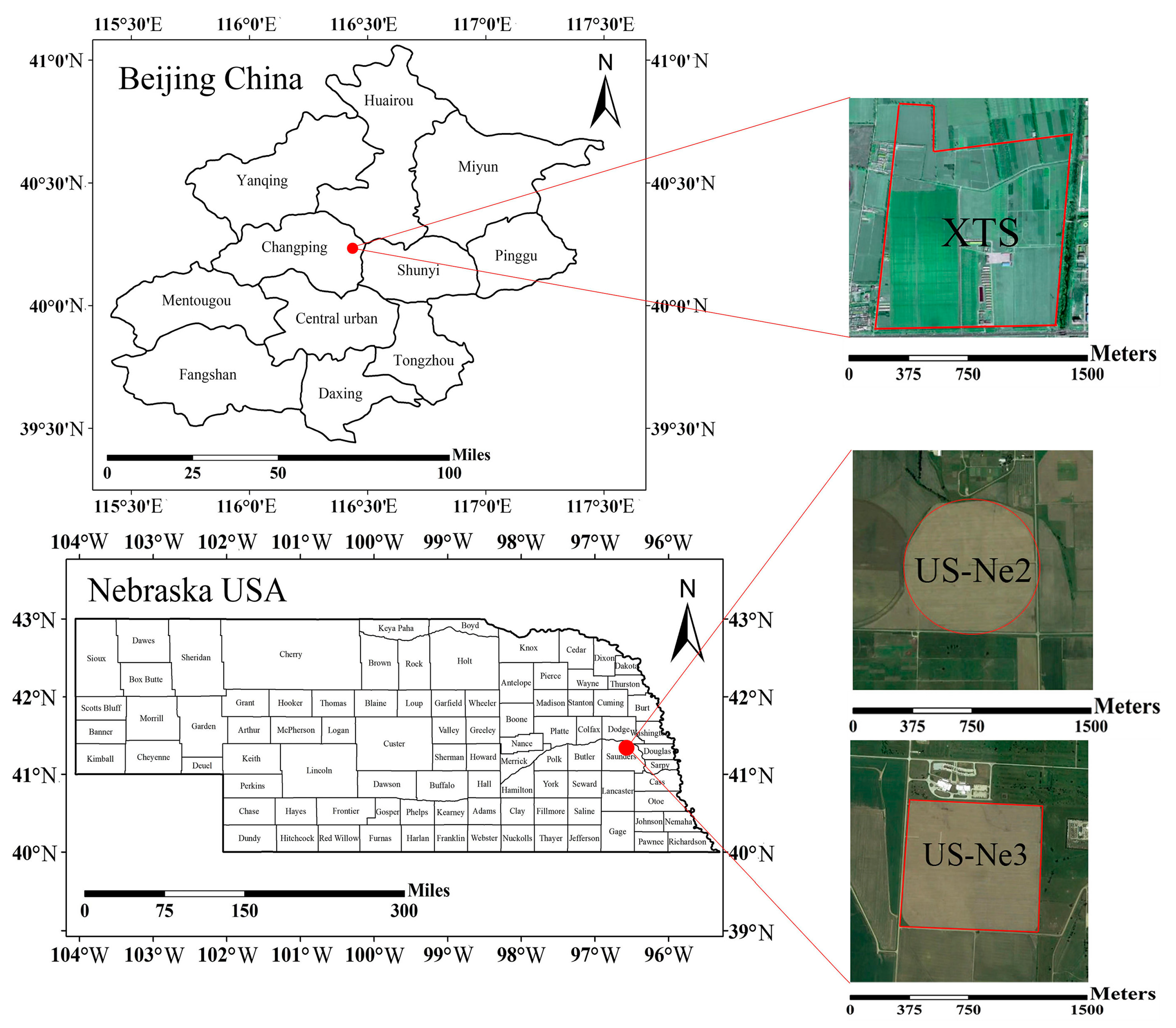
Figure 1 illustrates the spatial distribution of the two study sites. The first was located at the National Station for Precision Agriculture, Xiaotangshan (XTS), Beijing, China (40°10′48″N, 116°26′24″E). In 2002 and 2004, the biophysical parameters for winter wheat were determined through field and laboratory measurements: in the 2002 campaign, 48 plots 32.4 m × 30 m in size were used, along with three winter wheat varieties, while in 2004, 42 plots 32.4 m × 30 m in size were used and 21 winter wheat varieties were planted [30,42]. The other two study areas (US-Ne2 and US-Ne3) were situated at the University of Nebraska-Lincoln, NE, USA (41°9′54″N, 96°28′12″W; 41°10′47″N, 96°26′23″W). The US-Ne2 and US-Ne3 sites covered an area of about 65 ha, and featured a soybean (even years) and maize (odd years) crop rotation. The two sites had different levels of water stress that affected the crops (more details about these sites can be found in [43]). The biophysical parameters for the soybean crops were measured from June to September in 2002 and 2004 at the US-Ne2 site, and from June to September in 2002 at the US-Ne3 site. Table 1 provides additional information for the three sites.
2.2. Field Measurements
2.2.1. Canopy Reflectance Measurements
The canopy reflectance at the XTS site was measured using an ASD FieldSpec Pro spectrometer (Analytical Spectral Devices, Boulder, CO, USA) with a spectral range of 350–2500 nm and spectral resolutions of 3 nm (350–1050 nm) and 10 nm (1050–2500 nm). The measurements were obtained between 10:00 and 14:00 local time during clear and cloudless conditions, at a height of 1.3 m above the wheat canopy, with a 25° field of view. The average canopy reflectance for each plot was obtained via 20 individual measurements [30]. The canopy spectral reflectance at the US-Ne2 and US-Ne3 sites was obtained using two inter-calibrated Ocean Optics USB2000 radiometers (Ocean Optics Inc., Dunedin, FL, USA) ranging from 400 to 1100 nm in spectral range, with a spectral resolution of 1.5 nm [44]. One radiometer upwardly measures the upwelling radiance of the crop at a height of about 5.5 m above the canopy with a 25° field of view. The other downwardly measured the incident irradiance with a hemispherical field of view. The measurements were taken under clear sky conditions between 11:00 and 14:00 local time, and the reflectance was then calculated using methods described by Gitelson [1].
2.2.2. Measurement of Canopy Chlorophyll Content
At the XTS site, fresh wheat leaf samples were taken from the top of the canopy in a 1 m2 area for each plot [30], and rapidly placed in a plastic box containing ice for transport to the laboratory. The chlorophyll concentration was determined using a spectrophotometer [45]. The LAI of the sample leaves was measured using the dry-weight method [46]. At the US-Ne2 and US-Ne3 sites, fresh leaves from the soybean plants were collected in six small plots (20 m × 20 m) within each site. The leaf pigment was extracted with 80% acetone and LCC was obtained using a spectrophotometer [47]. The LAI of sample leaves was measured using an area meter (Model LI-3100, Li-Cor Inc., Lincoln, NE, USA) [43]. LCC and LAI for six plots were then averaged as site-level values. The total chlorophyll parameter for the CCC was calculated by multiplying the LAI by the LCC. The statistical analyses of the measured wheat and soybean CCCs are shown in Table 2.
2.3. ENVISAT MERIS Data
MERIS is an imaging spectrometer with a medium-spectral resolution onboard the ENVISAT platform of the European Space Agency (ESA). The instrument can sample surface reflectance in fifteen spectral bands with a range of 415–900 nm and has a temporal revisit time of 2–3 days. The data represent 15 spectral bands in the visible, near-infrared, and shortwave infrared regions with a spatial resolution of 300 m. The detailed specifications of the MERIS sensor are shown in Table 3. In this study, full-resolution surface reflectance products (for 25 June–24 September 2004), were produced by seven-day temporal synthesis from data collected at the original 2–3-day revisit frequency. The MERIS surface-reflectance product provides 13 bands, with bands 11 and 15 removed.
2.4. Vegetation Indices
Several LAI-VIs were selected to introduce LAI information into the MTCI. The normalized difference vegetation index (NDVI) was used for comparison, which exhibits saturation for different crops when the LAI is >2 [48,49,50]. Several researchers have modified the NDVI to mitigate the effect of saturation when estimating the LAI. A linearized NDVI (LNDVI) was derived by introducing a linearity-adjustment factor, β, into the NDVI equation. The LNDVI is more sensitive to spectral angles (reflectances) and has denser isolines with an increase in spectral angles (VI values) from the red to near infrared (NIR) space. Therefore, it has improve linearity and maintains a higher sensitivity to the fraction of the vegetation in densely vegetated areas [22]. Liu et al. [51] presented a stretched NDVI (S-NDVI) that was constructed using a scaling transformation function to eliminate saturation when the vegetation fraction became too large. In comparison with the NDVI, the S-NDVI did not reach saturation for LAIs of 2.5–5.0. In addition to such modified NDVIs, other spectral indices also maintain better relationships with the LAI for densely vegetated regions. The renormalized difference vegetation index (RDVI) [52] was proposed to combine the advantages of the difference vegetation index (DVI) [53] for low LAIs and those of the NDVI for high LAIs. Tan et al. [54] compared 56 hyperspectral vegetation indices and concluded that the RDVI had the greatest positive relationship with the LAI, and remained far from saturation in the presence of large LAIs. Haboudane et al. [16] designed a new triangular vegetation index (MTVI2) that proved to be the best predictor of the LAI. The MTVI2 was found to be insensitive to changes in chlorophyll and did not exhibit saturation at high LAIs. The vegetation indices used in this study are shown in Table 4.
2.5. Simulation of Canopy Reflectance Using the PROSAIL-D Model
The PROSAIL-D model was derived by coupling the PROSPECT-D leaf optical properties model [56] with the 4SAIL canopy bidirectional reflectance model [57]. The PROSAIL-D model was used to simulate MERIS observations and model the CCC based on VIs. It simulates upward and downward hemispherical radiation fluxes between 400 and 2500 nm with seven input parameters, and outputs the leaf spectral reflectance and transmittance. The 4SAIL model is used to simulate canopy reflectance with a series of input parameters. The input parameters for the PROSAIL-D model are shown in Table 5.
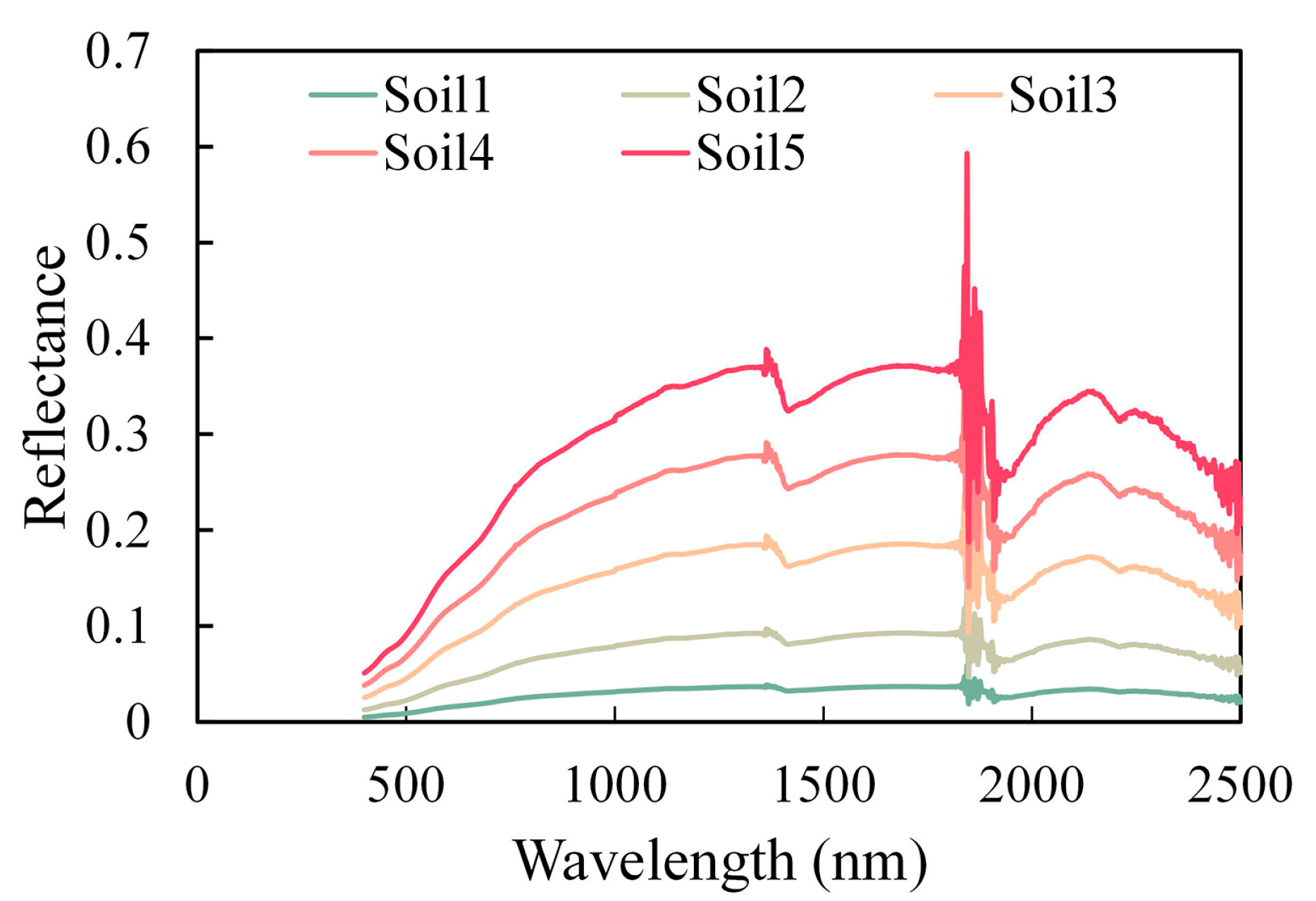
As shown in Table 5, the LCC values were set between 10 and 80 μg cm−2, at 10 μg cm−2 intervals. The leaf carotenoid content was set to 25% of the LCC due to its insensitivity to red and red-edge region reflectance. The LAI values ranged from 0.25 to 8, representing different levels of vegetation coverage. Five different leaf inclinations and five types of soil reflectance (Figure 2) were used to represent different canopy structures and soil backgrounds, respectively. The five types of soil reflectance were determined using the field-measured spectra of bare, dry soil multiplied by different brightness coefficients. The fraction of diffuse incoming solar radiation (skyl) was calculated in the PROSAIL-D model according to the solar zenith angle. The solar zenith angles were set between 0 and 60°, at 10° intervals. The remaining fixed parameters were set according to either field measurements or the scientific literature [58].
A dataset with 19,600 simulations was generated by running the PROSAIL-D model in Matlab (The Math Works, Natick, MA, USA). The simulated reflectance derived from the PROSAIL-D model was converted into the corresponding band reflectance using the MERIS spectral response function [59].
2.6. CCC Retrieval Model
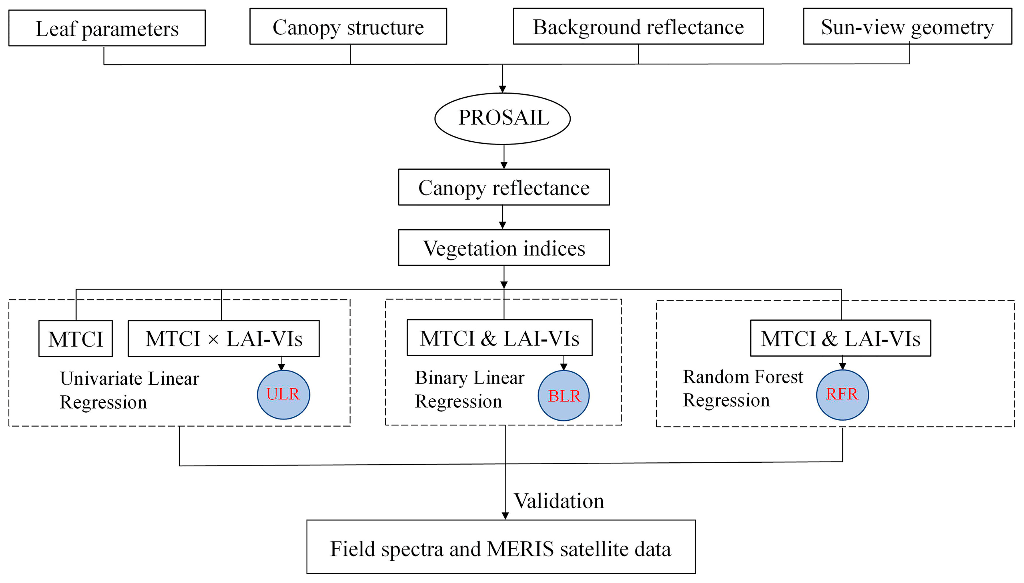
Three distinct methods were used to estimate CCC to retrieve CCC using VIs based on simulated canopy spectrum data from the PROSAIL-D model. Figure 3 summarizes the steps in retrieving canopy chlorophyll. The published VIs calculated from the simulated canopy reflectance were used based on the PROSAIL-D model presented in this study. First, linear regression was used to assess the relationships between CCC and the VIs. A random forest regression approach trained with VIs was then employed to estimate the CCC. Finally, field measurements and MERIS satellite data were used to validate the three types of constructed model.
2.6.1. Linear Regression Analysis
The performance of the combined VIs was assessed using simple linear regression. Firstly, univariate linear regression (ULR) was employed to model the relationship between the CCC and MTIC, MTCI × NDVI, MTCI × LNDVI, MTCI × SNDVI, MTCI × RDVI, and MTCI × MTVI2. Binary linear regression (BLR) models were then constructed in Matlab based on the relationship between CCC and the MTCI and NDVI, MTCI and LNDVI, MTCI and SNDVI, MTCI and RDVI, and MTCI and MTVI2. We used the coefficient of determination (R2), root mean square error (RMSE), bias (Bias), and normalized RMSE (NRMSE) to evaluate the fitness and predictive power of the models, respectively. They were calculated as follows:
where is the predicted CCC, is the measured CCC, is the average measured CCC, is the maximum value of the CCC, is the minimum value of the CCC, and n is the number of measurements used. While linear regression analysis is simple to implement, particularly in uncomplicated variable spaces, complex vegetated areas are likely to require more advanced methods for their analysis.
2.6.2. Implementing the Random Forest Regression Approach
Random forest is an ensemble learning method that combines multiple decision trees for classification or regression [60]. It runs efficiently on large datasets with excellent performance and accuracy [38,61]. In this study, recursive partitioning was employed to divide the simulated dataset into 100 homogeneous subsets (100 trees), and the results of all the trees were then averaged. A random forest regression (RFR) was implemented in Matlab with the use of the MTCI and LAI-VIs as input features for estimating CCC. The CCC models were validated using ground spectral measurements and MERIS satellite data.
3. Results
3.1. Sensitivities of Spectra and MTCI to LAI and CCC
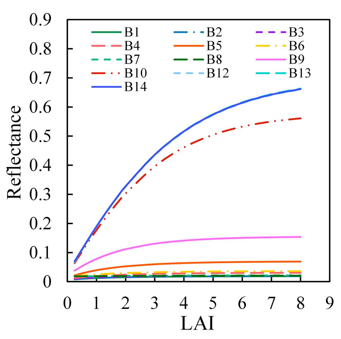
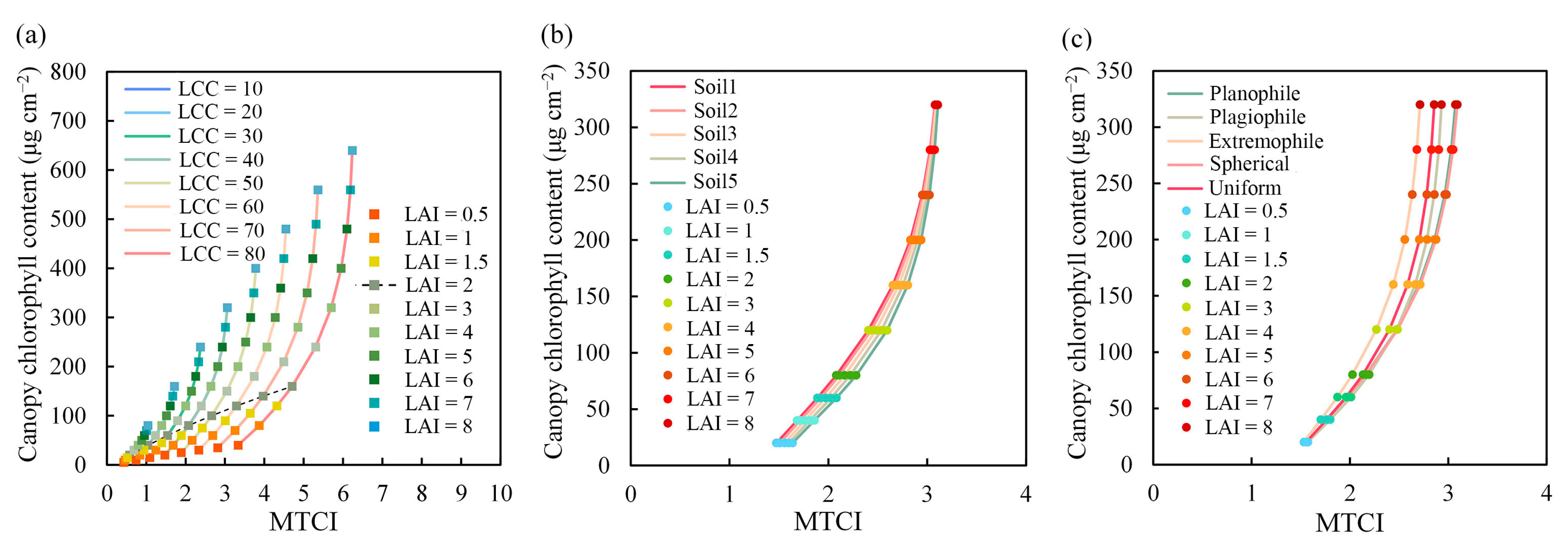
Figure 4 shows that all of the MERIS bands reached saturation due to the increase in LAI, particularly in the visible region, with bands 7 and 8 being the most severe, but the effect was slightly mitigated in the near-infrared region. The relationship plot for MTCI and CCC suggests that the saturation during CCC retrieval was largely caused by the LAI (Figure 5a). Figure 5a provides an overview of the saturation effect observed for the MTCI when the LAI is >2 at different LCCs. In summary, these results suggest that higher LAIs largely contributed to the abnormal saturation of the spectra and MTCI. The soil background and average leaf angle also affected the retrieval of the CCC based on the MTCI. Figure 5b suggests that the soil background had little impact on the MTCI and CCC estimation, especially at high LAIs. This was because the canopy reflectance contained less background reflectance due to the increase in vegetation coverage. By contrast, the effect of the average leaf angle increased with the LAI during CCC estimation, which was due to the influence of the complex canopy structure on the transmission of solar radiation (Figure 5c). Figure 5b,c also show that the LAI was the main cause of saturation for the MTCI.
3.2. CCC Estimation Using the Simulated Dataset
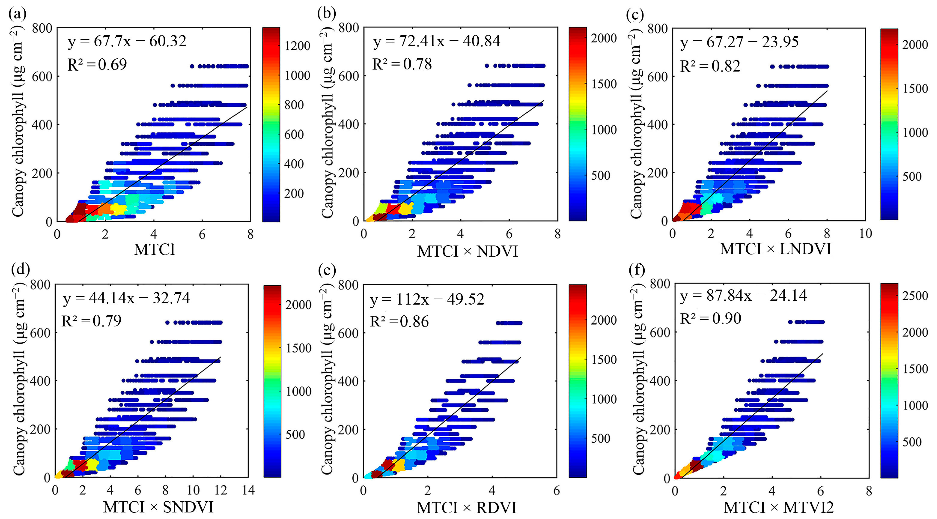
The univariate linear regressions between CCC and the models are shown in Figure 6. The R2 was selected to assess the ability of each model to prevent an ill-posed problem. By comparing Figure 6b–f with Figure 6a, it can be observed that the scatter plots for MTCI × LAI-VIs are more compact than for the MTCI, and the MTCI × LAI-VIs plots also feature more linear trends. MTCI × MTVI2 showed the best performance, with an R2 value (0.90) higher than that for the MTCI (0.69).
The binary linear regressions were employed in Matlab and the results were compared in Table 6. The R2 values were used to evaluate the predictive ability of each model and demonstrated a strong correlation between MTCI and LAI-VIs, and CCC. The binary regression models based on the MTCI and LAI-VIs were more representative than the univariate regression model using the MTCI alone. MTCI and RDVI (R2 = 0.82), and MTCI and MTVI2 (R2 = 0.80) had similar results, with excellent performance. However, the overall results for the binary regression models (Table 6) indicate reduced performance compared to the univariate regression models (Figure 6).
The random forest approach was also tested, using the MTCI and LAI-VIs as inputs, for retrieving the CCC. The R2 was selected to assess the predictive ability of each model, as shown in Table 7, where it is apparent that the CCC exhibits strong correlations with the MTCI and LAI-VIs with the RFR approach. The R2 values are higher than for the two types of linear regression.
3.3. Validation of CCC Estimation Using Field Canopy Spectral Measurements
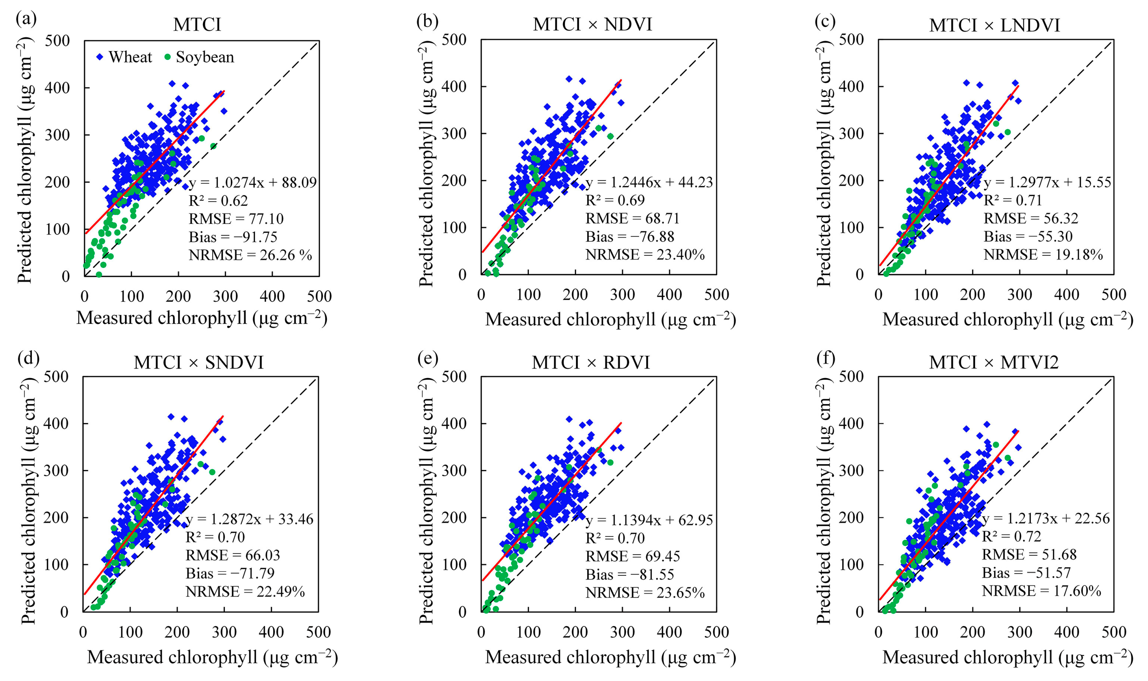
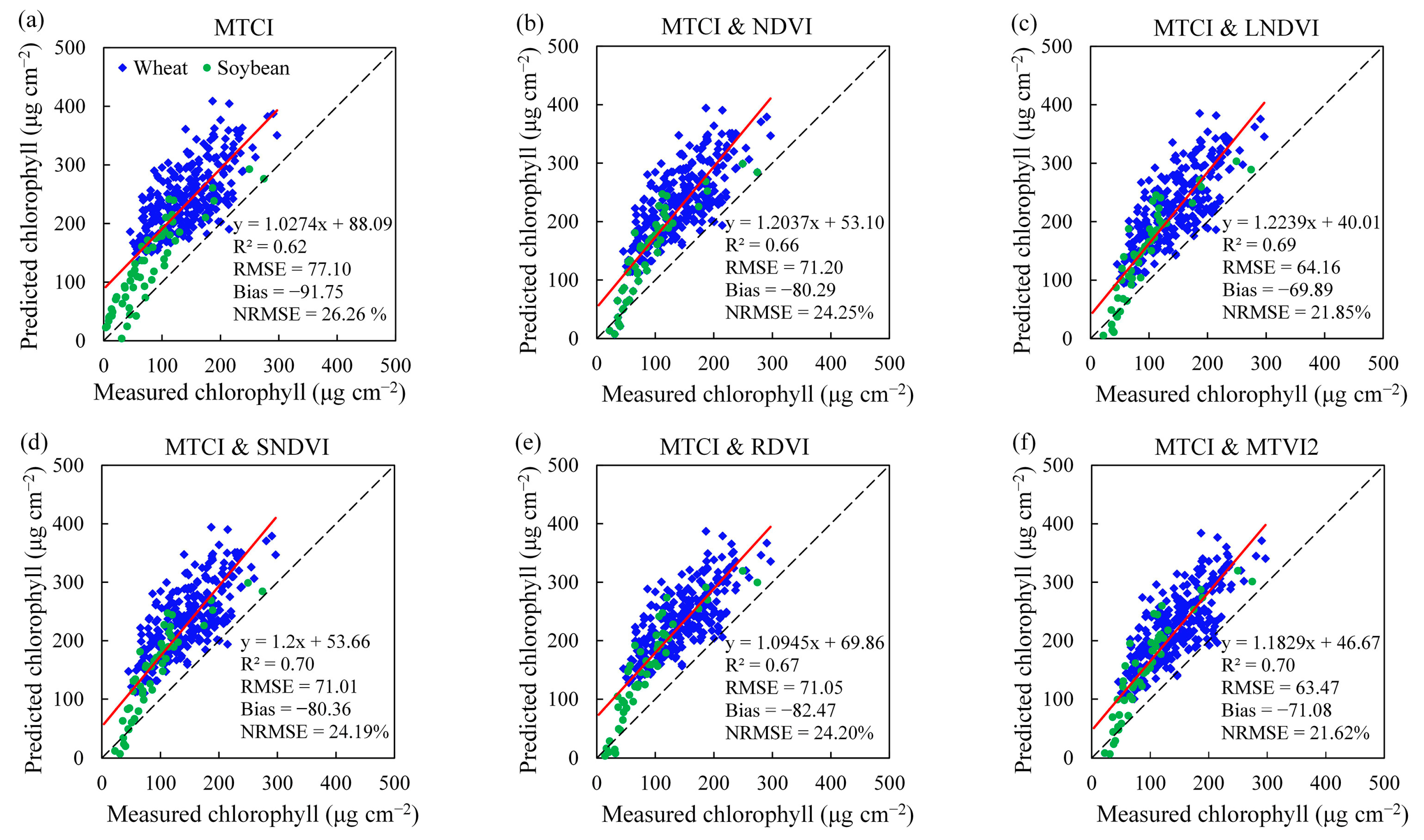
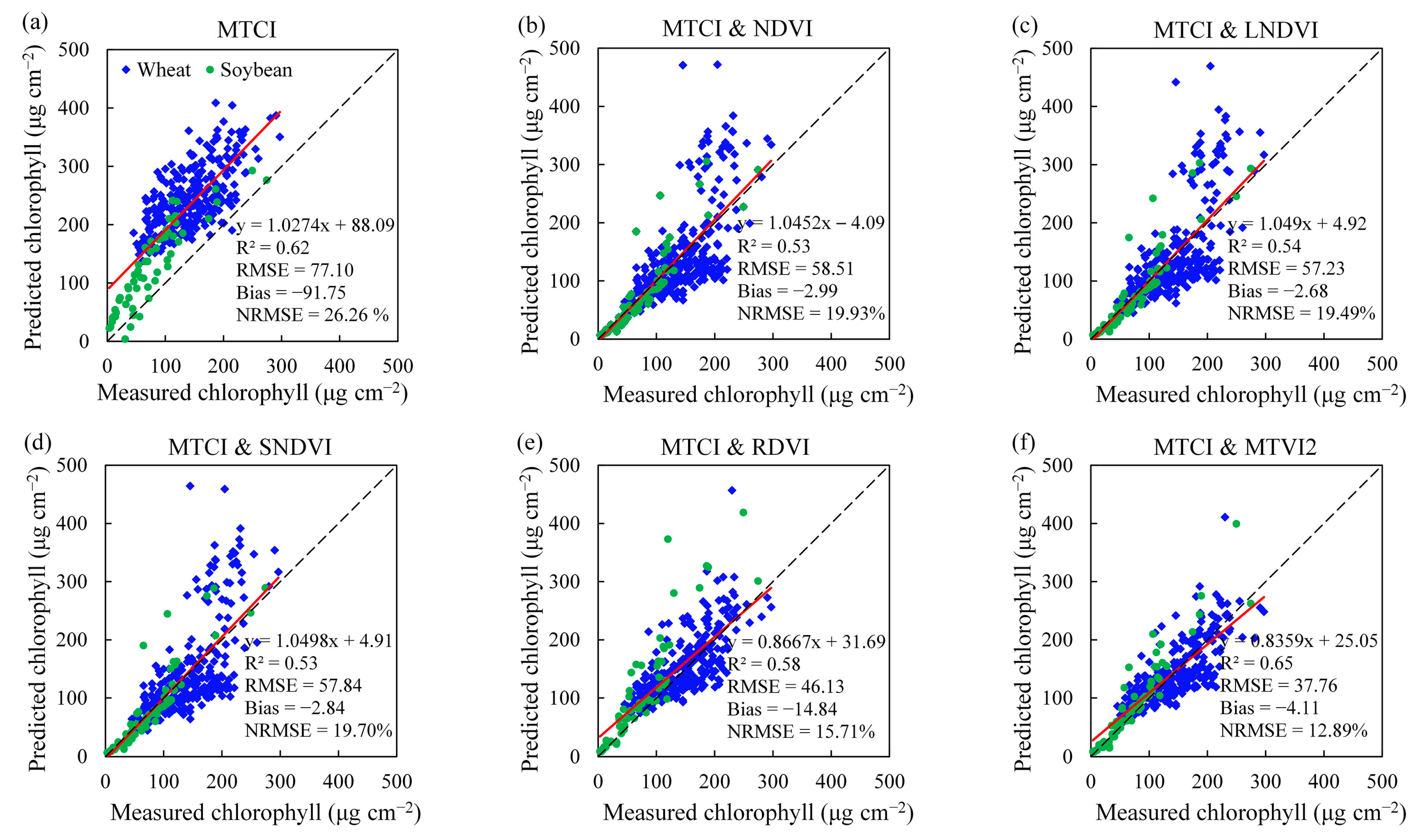
Each model was evaluated by computing the RMSE between the field measurements and CCC values predicted based on the field canopy reflectance data. All of the selected VIs were calculated from field canopy spectra data that was resampled according to MERIS band settings. Figure 7, Figure 8 and Figure 9 display the scatter plots for the predicted and true values produced by the models. As shown in Figure 7, the accuracy for MTCI × LAI-VIs was higher than that for the MTCI, and MTCI × MTVI2 showed the best performance (R2 = 0.72, RMSE = 51.68 μg cm−2, Bias = −51.57 μg cm−2, and NRMSE = 17.60%). The results for the BLR model (Figure 8) suggest that the MTCI and LAI-VIs performed better than the MTCI alone; however, the performance was not comparable to that of the combined VIs with ULR. Both the ULR and BLR approaches universally overestimated the CCC, and this effect was most prominent with BLR. Thus, these methods cannot compensate for ill-posed VIs. Figure 9 indicates that the RFR approach performed the best with the scatter points much closer to a 1:1 linear pattern, especially for the soybeans. A comparison of all the models revealed that the random forest regression model trained using binary variables based on MTCI and MTVI2 showed the best performance (R2 = 0.65, RMSE = 37.76 μg cm−2, Bias = −4.11 μg cm−2, and NRMSE = 12.89%). Therefore, the random forest regression model trained with binary variables based on the MTCI and LAI-VIs could effectively alleviate the influence of ill-posed VIs on the accuracy of CCC estimation.
3.4. Validation of CCC Estimation from MERIS Satellite Data
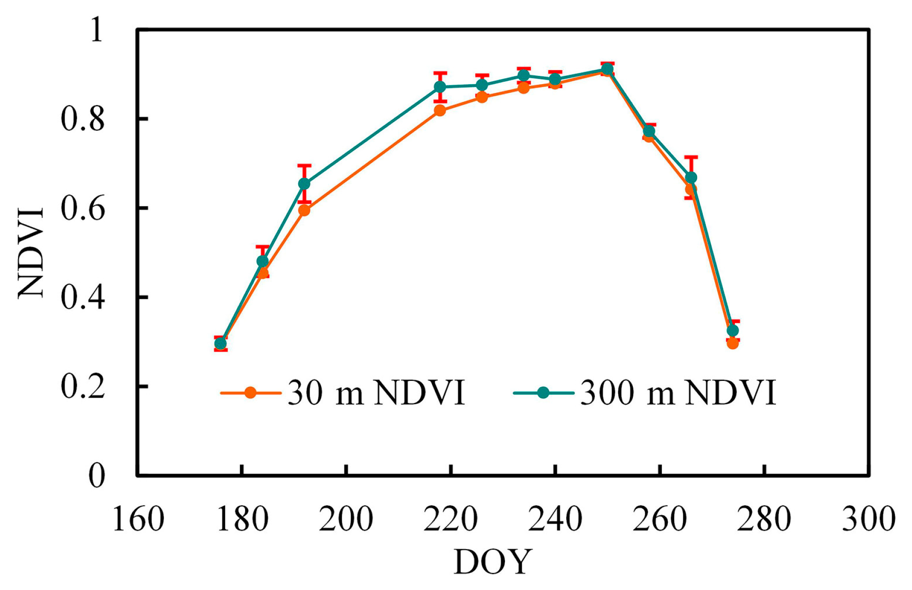
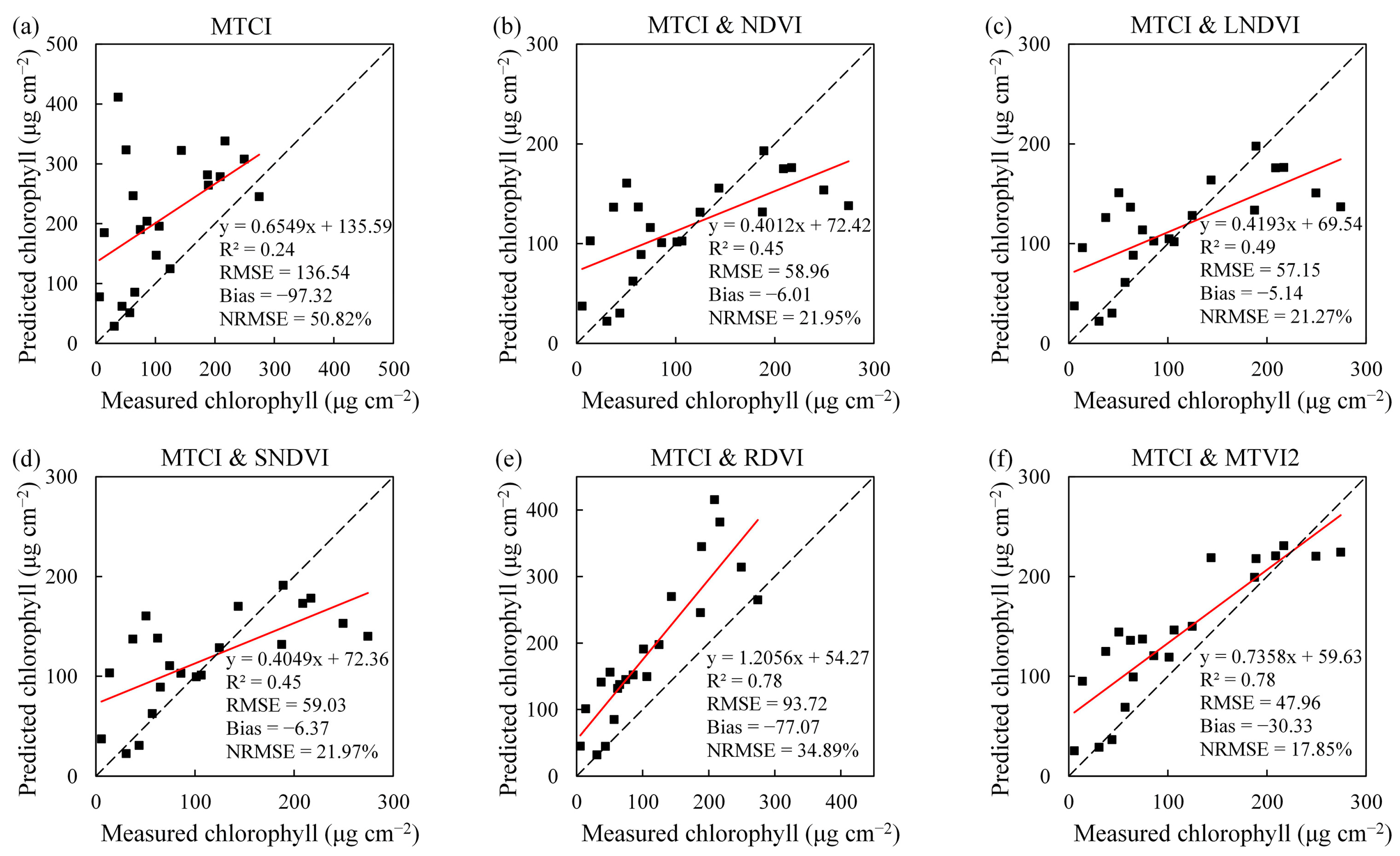
The MERIS satellite data obtained from the US-Ne2 site in 2004 were used to validate the reliability and accuracy of the built models. The measurements from the XTS site were not used due to the lack of sufficient time-series data. Figure 10 shows Landsat NDVI time-series data of different resolutions at the US-Ne2 site in 2004. The 30 m Landsat NDVIs are consistent with the mean NDVIs derived from the 300 m-pixel MERIS data, which indicates the uniform growth of the soybeans at the site. Therefore, we used the ground-measured CCC to assess the usefulness of the MERIS spectral data for retrieving CCC. Table 8 shows the CCC estimation results for the three approaches. The VI-combination methods were found to be more accurate than using MTCI alone (R2 = 0.24; RMSE = 136.54 μg cm−2). However, there was a limited improvement in accuracy when using the ULR and BLR approaches. These approaches showed reduced performance in alleviating the negative influence of the VIs on CCC estimation. However, the RFR approach resulted in good prediction accuracy. The relationship between the predicted and measured CCC for the RFR approach is shown in Figure 11. The validation results for the MTCI and LAI-VIs were better than those for the MTCI alone, and the MTCI and MTVI2 showed the best performance, achieving an accuracy of R2 = 0.78, and RMSE = 47.96 μg cm−2. It should be noted that the above analysis and conclusions were based on ground and satellite-based measurements.
4. Discussion
4.1. Role and Form of VI Combinations in CCC Estimation Models
The CCC is related to the LAI and LCC, and the estimation of chlorophyll content with remote sensing requires information on both variables [62]. The chlorophyll index mainly uses red-edge bands that are sensitive to LCC [10,13], while LAI-VIs use near-infrared bands that are sensitive to the LAI [16,52,55]. The MTCI and LAI-VIs were combined to improve the remote sensing of CCC for crops, in this study. The results indicate that the above VI combinations, with all three of the selected regression models, performed better in estimating the CCC than the MTCI alone. This implies that the VI combinations effectively fused the leaf area index and chlorophyll information.
The type of VI combination that is appropriate depends on whether the estimated vegetation parameter is at the canopy or leaf level. A combined multiplicative VI was used for the univariate regression model. Similarly to in this study, a SAR and optical multiplication vegetation index (SOMVI) has been proposed to improve the estimation of above ground biomass [63]. Several combined VIs based on CHL-VIs and LAI-VIs have also been proposed for LCC estimation using a univariate regression model [28,29,30]. Canopy biomass is a canopy population parameter that is similar to CCC, while LCC is a leaf-level chlorophyll parameter that is independent of the LAI. The combined VIs that are used for LCC estimation are often in the form of ratio indices such as TCARI/OSAVI [28], which reduces the influence of the LAI on the VI. However, multiplicative forms, such as the one used in this study, are not typically used.
The best VI combination can also differ according to the type of regression analysis model. Multiple regression or advanced machine-learning techniques can be used with more input variables to describe complex scenarios. For example, this study used a CHL-VI and a LAI-VI as binary variables for binary regression and the random forest model for CCC estimation. Multiple vegetation indices can also be used in the cost function to estimate vegetation parameters based on the direct inversion of the vegetation model [31]. For estimating the LCC in crops, a simple LUT (look-up table) has been proposed that is indexed using a CHL-VI and LAI-VI [31]. This matrix-based VI combination is a special form of physical model inversion, and has been proven to be better than linear regression models that use a VI with a single ratio. Clevers [12] used MTCI to estimate the CCC of soybeans based on linear regression and field spectra, achieving an RMSE of 86 μg cm−2, similar to the result were obtained using the MTCI alone (RMSE = 77.10 μg cm−2). However, when using a combination of the MTCI and LAI-VI with three regression techniques, our results were far better, and the best performance for three regression approaches were RMSE = 51.68 μg cm−2 (ULR), RMSE = 63.47 μg cm−2 (BLR), and RMSE = 37.76 μg cm−2 (RFR). The results presented in this paper confirm that multiple regression models that integrate CHL-VIs and LAI-VIs, especially the random training model, show better generalization performance than the use of a single CHL-VI.
4.2. Influence of LAI-VIs Selection of VI Combinations
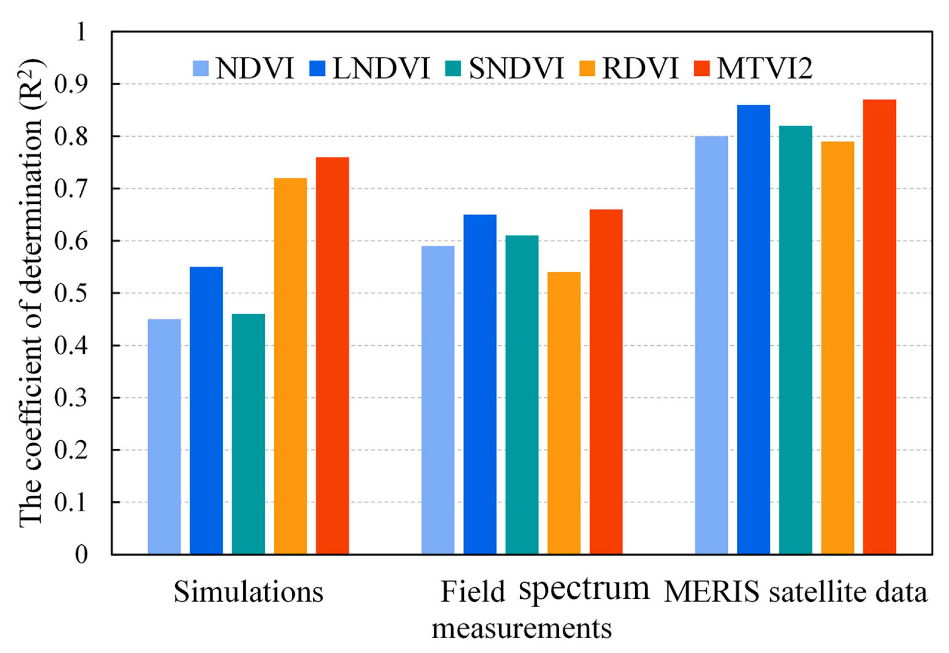
The key to the success of the combined approach employed was the excellent performance of the LAI-VIs in reducing the saturation associated with high LAIs. The combination of the MTCI and LAI-VIs resulted in a greater sensitivity to CCC compared to the use of a single MTCI. As shown in Figure 5, high LAIs are the main cause of saturation when estimating CCC. The purpose of adding LAI-VIs is to increase the sensitivity of the MTCI to a high CCC in the presence of a high LAI. Therefore, we investigated the performance of each VI combination in CCC estimation. The results in Section 3.3 and Section 3.4 show that the modified NDVIs, especially the LNDVI, performed better than the NDVI. The RDVI and MTVI2, which also proved to be resistant to saturation, were used in the combined VIs and performed better than the NDVI. The sensitivity of LAI-VIs to high LAIs can affect the performance of the training regression model. The relationships between LAI-VIs and the LAI can also be affected by other factors such as canopy coverage, as demonstrated in previous studies, and different LAI-VIs can have different capabilities for estimating the LAI [28,64,65]. The MTVI2 is a modification of the triangular vegetation index (TVI) that preserves the sensitivity at high LAIs and reduces the effects of soil contamination [16]. The relationships between the LAI and LAI-VIs based on the simulated spectra, field spectra, and MERIS satellite data are shown in Figure 12: the MTVI2 was more closely related to the LAI than the other LAI-VIs were, in agreement with previous studies. This might be why the combined VI that included the MTVI2 showed the best results.
4.3. Comparing the Performance of the Proposed CCC Estimation Models for Satellite Data with Variable LAIs
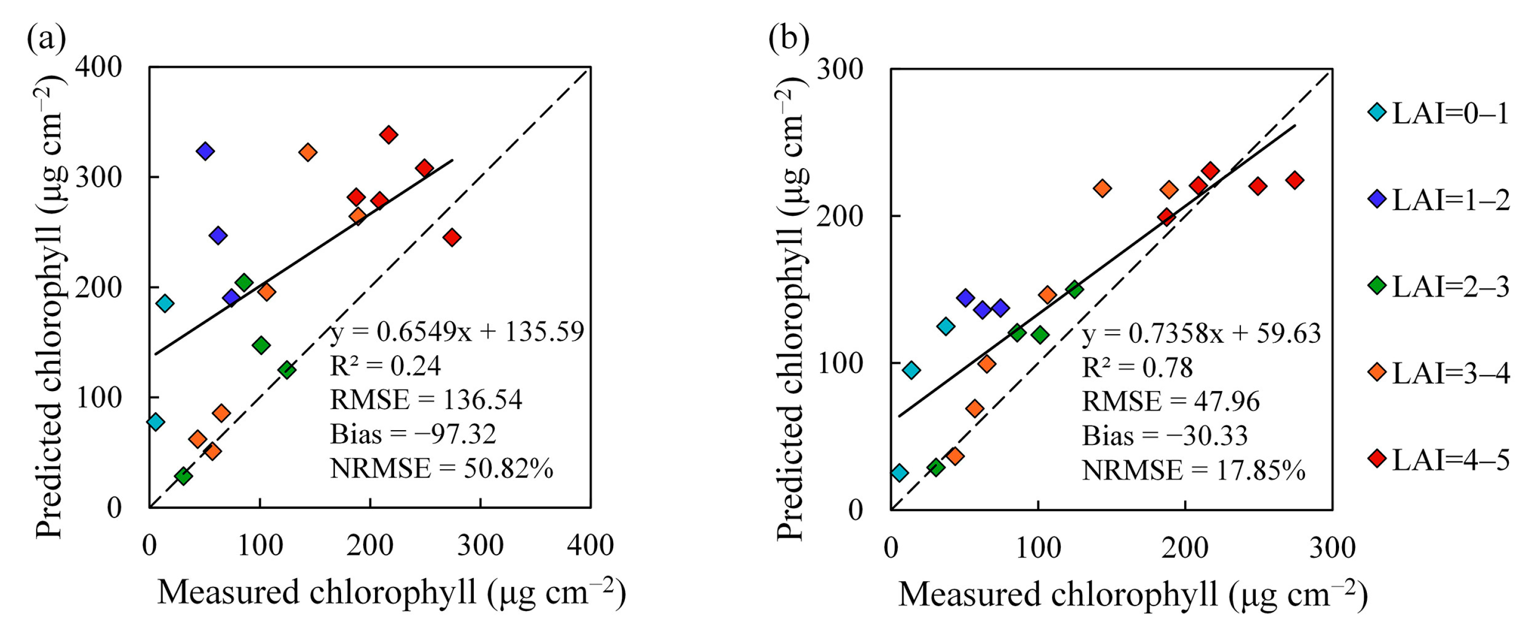
It is important to examine the performance of models for CCC estimation when using satellite data. Satellite data are affected by several factors such as noise and neighboring effects. It is still challenging to apply retrieval models to satellite data [66]. The results from this study, which only used the MTCI, confirm the findings from previous studies showing that low-LAI and high-LAI conditions can cause difficulties when using VIs to estimate vegetation chlorophyll [19,20,21,24]. The results indicate that the RFR model using a VI combination showed the best improvement in CCC estimation, while the performance improvement for MERIS satellite data varied for different LAI values (Figure 13b). The scatter points in Figure 13b are closer to a 1:1 line when LAI > 2, indicating that the MTCI and MTVI2 combination (using random forest regression) could reduce the overestimation of CCC that occurred when using the MTCI alone in the ULR model at high LAIs (Figure 13a). The proposed RFR method improved the large overestimation of values. However, some overestimation still occurred at low LAIs (LAI < 2) (Figure 13b). This is mainly because the chlorophyll VI calculated based on red-edge reflectance was affected by the soil background more than the NIR band when the canopy was sparse or at low coverage [25].
4.4. Limitations of Model Simulations and Validation Data
This study was mainly aimed at enhancing the sensitivity of the MTCI to both leaf chlorophyll information and the LAI for CCC estimation. Therefore, wide ranges for the LCC, LAI, canopy structure, and soil background were used in the PROSAIL simulation to analyze the performance of the LAI-VIs and MTCI combination approach. In this study, the leaf parameters, such as the N, Cw, and Cm, were set to the defaults for wheat and soybean crops (Table 5). The variations of other leaf parameters were of little significance for evaluating the effects of the proposed methods for fusing LAI and chlorophyll information. However, these parameters may affect the CCC estimation models for different crops based on spectrum simulations. Previous studies have demonstrated that Cw has little influence on the visible and red-edge bands commonly used for vegetation chlorophyll estimation [67], while N and Cm can affect chlorophyll estimation [27,68,69]. The leaf parameters, such as N, should be adjusted according to the specific crop type if the proposed VI combination approach is applied to other crops.
Although this study considered the variation in the solar zenith angle to represent daily and seasonal changes, the simulations and test data used for the modeling and validation were limited to nadir observations. The ground spectrum was obtained at the nadir, and the seven-day 300 m surface-reflectance MERIS product lacked information on the view zenith angle. Therefore, the simulation data in this study were also based on nadir observations. However, remote sensing data, especially satellite imagery, widely vary in the zenith angle. MERIS reflectance data may not be observed from a nadir or near-nadir view [70], which increases the uncertainty of the validation results for the MERIS satellite data. Although the view zenith angle was fixed as a nadir observation, the results from the simulated field and MERIS data all show the effectiveness of the proposed VI combination method for CCC estimation. The influence of the view zenith angle on different CCC estimation models should be evaluated in the future.
Although ENVISAT MERIS is no longer in work, it makes sense to use past data to produce products with long time series. In addition, Sentinel-3 OLCI is the successor to MERIS, and they have the same band settings and similar spectral response functions [58]. Therefore, the CCC retrieval methods developed for MERIS can generally be applied to Sentinel-3 datasets. In the future, we hope to take the synchronous measurement for Sentinel-3 and further test our algorithm.
5. Conclusions
This paper proposes a combination of the MTCI and LAI-VIs for univariate linear, binary linear, and random forest regression that fuses leaf area index and chlorophyll information to improve the retrieval of CCC based on the PROSAIL-D model. The validation results based on both field spectra and MERIS satellite data reveal that the vegetation index combinations for all three regression models effectively improved the accuracy, although the VI combination can vary for different types of regression analysis models. The combined multiplicative VI, MTCI × MTVI2, showed a better performance for the univariate regression model (field spectra for soybeans and wheat: RMSE = 51.68 μg cm−2; MERIS satellite data for soybeans: RMSE = 88.44 μg cm−2) than the MTCI alone (field spectra: RMSE = 77.10 μg cm−2; MERIS satellite data: RMSE = 136.54 μg cm−2). Moreover, combining the MTCI and LAI-VIs into the random forest regression models exhibited greater potential for retrieving the CCC than the two linear regression models. The MTCI and MTVI2 combination with random forest regression performed the best, achieving an RMSE of 37.76 μg cm−2 for the field spectra data, and an RMSE of 47.96 μg cm−2 for the MERIS satellite data. This study indicates that random forest regression models with a combination of the MTCI and LAI-VIs have an advantage in the fusion of LAI and leaf chlorophyll information, and can produce accurate and robust estimates for CCC. Due to its simplicity, the single combined multiplicative VI with an empirical regression model also shows potential for estimating CCC. The vegetation index combination method proposed in this paper can be applied to other chlorophyll-related vegetation indices to improve their performance in CCC estimation. Since the simulation data used in this paper were mainly related to wheat and soybean crops, the above-described model for CCC retrieval based on simulated datasets must be adjusted according to vegetation type.
Author Contributions
Conceptualization: Q.S. and Q.J.; methodology: Q.S. and Q.J.; validation: Q.S.; formal analysis: Q.S., and Q.J.; investigation: L.L.; data curation: Q.S. and X.Q.; writing—original draft preparation: Q.S.; writing—review and editing: X.L.; visualization: Q.S.; supervision: L.L. and H.D. All authors have read and agreed to the published version of the manuscript.
Funding
This research was funded by the National Key Research and Development Program of China, grant number 2017YFA0603001, and the National Natural Science Foundation of China, grant number 42071330 and 41825002.
Institutional Review Board Statement
Not applicable.
Informed Consent Statement
Not applicable.
Data Availability Statement
All data used in this study were from open access satellite products or published field work cited in this article.
Acknowledgments
We appreciate the data provided by the Center for Advanced Land Management Information Technologies (CALMIT), University of Nebraska–Lincoln.
Conflicts of Interest
The authors declare no conflict of interest.
References
- Gitelson, A.A.; Viña, A.; Verma, S.B.; Rundquist, D.C.; Arkebauer, T.J.; Keydan, G.; Leavitt, B.; Ciganda, V.; Burba, G.G.; Suyker, A.E. Relationship between gross primary production and chlorophyll content in crops: Implications for the synoptic monitoring of vegetation productivity. JGR Atmos. 2006, 111, D08S11. [Google Scholar] [CrossRef] [Green Version]
- Croft, H.; Chen, J.M.; Luo, X.; Bartlett, P.; Chen, B.; Staebler, R.M. Leaf chlorophyll content as a proxy for leaf photosynthetic capacity. Glob. Chang. Biol. 2017, 23, 3513–3524. [Google Scholar] [CrossRef] [PubMed]
- He, R.; Li, H.; Qiao, X.; Jiang, J. Using wavelet analysis of hyperspectral remote-sensing data to estimate canopy chlorophyll content of winter wheat under stripe rust stress. Int. J. Remote Sens. 2018, 39, 4059–4076. [Google Scholar] [CrossRef]
- Gitelson, A.A.; Peng, Y.; Arkebauer, T.J.; Schepers, J. Relationships between gross primary production, green LAI, and canopy chlorophyll content in maize: Implications for remote sensing of primary production. Remote Sens. Environ. 2014, 144, 65–72. [Google Scholar] [CrossRef]
- Lichtenthaler, H.K.; Wellburn, A.R. Determinations of total carotenoids and chlorophylls a and b of leaf extracts in different solvents. Biochem. Soc. Trans. 1983, 603, 591–592. [Google Scholar] [CrossRef] [Green Version]
- Wu, C.; Wang, L.; Niu, Z.; Gao, S.; Wu, M. Nondestructive estimation of canopy chlorophyll content using Hyperion and Landsat/TM images. Int. J. Remote Sens. 2010, 31, 2159–2167. [Google Scholar] [CrossRef]
- Darvishzadeh, R.; Matkan, A.A.; Dashti Ahangar, A. Inversion of a radiative transfer model for estimation of rice canopy chlorophyll content using a lookup-table approach. IEEE J. Sel. Top. Appl. Earth Observ. Remote Sens. 2012, 5, 1222–1230. [Google Scholar] [CrossRef] [Green Version]
- Clevers, J.G.P.W.; Kooistra, L. Using hyperspectral remote sensing data for retrieving canopy chlorophyll and nitrogen content. IEEE J. Sel. Top. Appl. Earth Observ. 2012, 5, 574–583. [Google Scholar] [CrossRef]
- Wu, C.; Niu, Z.; Tang, Q.; Huang, W. Estimating chlorophyll content from hyperspectral vegetation indices: Modeling and validation. Agric. For. Meteorol. 2008, 148, 1230–1241. [Google Scholar]
- Verrelst, J.; Camps-Valls, G.; Muñoz-Marí, J.; Rivera, J.P.; Veroustraete, F.; Clevers, J.G.P.W.; Moreno, J. Optical remote sensing and the retrieval of terrestrial vegetation bio-geophysical properties—A review. ISPRS J. Photogramm. Remote Sens. 2015, 108, 273–290. [Google Scholar] [CrossRef]
- Croft, H.; Chen, J.M.; Zhang, Y. The applicability of empirical vegetation indices for determining leaf chlorophyll content over different leaf and canopy structures. Ecol. Complex. 2014, 17, 119–130. [Google Scholar] [CrossRef]
- Clevers, J.G.P.W.; Gitelson, A.A. Remote estimation of crop and grass chlorophyll and nitrogen content using red-edge bands on Sentinel-2 and -3. Int. J. Appl. Earth Obs. Geoinf. 2013, 23, 344–351. [Google Scholar] [CrossRef]
- Dash, J.; Curran, P.J. The MERIS terrestrial chlorophyll index. IEEE J. Sel. Top. Appl. Earth Observ. 2004, 25, 5403–5413. [Google Scholar] [CrossRef]
- Gausman, H.W.; Allen, W.A.; Cardenas, R.; Richardson, A.J. Effects of leaf nodal position on absorption and scattering coefficients and infinite reflectance of cotton leaves, Gossypium hirsutum L. Agron. J. 1971, 63, 87–91. [Google Scholar] [CrossRef]
- Bausch, W.C. Soil background effects on reflectance-based crop coefficients for corn. Remote Sens. Environ. 1993, 46, 213–222. [Google Scholar] [CrossRef]
- Haboudane, D. Hyperspectral vegetation indices and novel algorithms for predicting green LAI of crop canopies: Modeling and validation in the context of precision agriculture. Remote Sens. Environ. 2004, 90, 337–352. [Google Scholar] [CrossRef]
- Jay, S.; Gorretta, N.; Morel, J.; Maupas, F.; Bendoula, R.; Rabatel, G.; Dutartre, D.; Comar, A.; Baret, F. Estimating leaf chlorophyll content in sugar beet canopies using millimeter-to centimeter-scale reflectance imagery. Remote Sens. Environ. 2017, 198, 173–186. [Google Scholar]
- Peng, Y.; Nguy-Robertson, A.; Arkebauer, T.; Gitelson, A.A. Assessment of canopy chlorophyll content retrieval in maize and soybean: Implications of hysteresis on the development of generic algorithms. Remote Sens. 2017, 9, 226. [Google Scholar] [CrossRef] [Green Version]
- Myneni, R.B.; Nemani, R.R.; Running, S.W. Estimation of global leaf area index and absorbed PAR using radiative transfer models. IEEE Trans. Geosci. Remote Sens. 1997, 35, 1380–1393. [Google Scholar] [CrossRef] [Green Version]
- Gitelson, A.A. Wide dynamic range vegetation Index for remote quantification of biophysical characteristics of vegetation. J. Plant Physiol. 2004, 161, 165–173. [Google Scholar]
- Ferrara, R.M.; Fiorentino, C.; Martinelli, N.; Garofalo, P.; Rana, G. Comparison of different ground-based NDVI measurement methodologies to evaluate crop biophysical properties. Ital. J. Agron. 2010, 5, 145–154. [Google Scholar] [CrossRef]
- Jiang, Z.; Huete, A.R. Linearization of NDVI based on its relationship with vegetation fraction. Photogramm. Eng. Remote Sens. 2010, 76, 965–975. [Google Scholar]
- Gu, Y.; Wylie, B.K.; Howard, D.M.; Phuyal, K.P.; Ji, L. NDVI saturation adjustment: A new approach for improving cropland performance estimates in the Greater Platte River Basin, USA. Ecol. Indic. 2013, 30, 1–6. [Google Scholar] [CrossRef]
- Ali, A.M.; Darvishzadeh, R.; Skidmore, A.; Gara, T.W.; O’Connor, B.; Roeoesli, C.; Heurich, M.; Paganini, M. Comparing methods for mapping canopy chlorophyll content in a mixed mountain forest using Sentinel-2 data. Int. J. Appl. Earth Obs. Geoinf. 2020, 87, 102037. [Google Scholar] [CrossRef]
- Broge, N.H.; Thomsen, A.G.; Andersen, P.B. Comparison of selected vegetation indices as indicators of crop status. In Proceedings of the 22nd Symposium of the European Association of Remote Sensing Laboratories, Pragua, Czech Republic, 4–5 June 2002. [Google Scholar]
- Daughtry, C.S.T.; Waltthall, C.L.; Kim, M.S.; de Colstoun, E.B.; McMurtrey, J.E. Estimating corn leaf chlorophyll concentration from leaf and canopy reflectance. Remote Sens. Environ. 2000, 74, 229–239. [Google Scholar] [CrossRef]
- Haboudane, D.; Tremblay, N.; Miller, J.R.; Vigneault, P. Remote estimation of crop chlorophyll content using spectral indices derived from hyperspectral data. IEEE Trans. Geosci. Remote Sens. 2008, 46, 423–437. [Google Scholar] [CrossRef]
- Haboudane, D.; Miller, J.R.; Tremblay, N.; Zarco-Tejada, P.J.; Dextraze, L. Integrated narrow-band vegetation indices for prediction of crop chlorophyll content for application to precision agriculture. Remote Sens. Environ. 2002, 81, 416–426. [Google Scholar] [CrossRef]
- Kooistra, L.; Clevers, J.G.P.W. Estimating potato leaf chlorophyll content using ratio vegetation indices. Remote Sens. Lett. 2016, 7, 611–620. [Google Scholar] [CrossRef] [Green Version]
- Cui, B.; Zhao, Q.; Huang, W.; Song, X.; Ye, H.; Zhou, X. A new integrated vegetation index for the estimation of winter wheat leaf chlorophyll content. Remote Sens. 2019, 11, 974. [Google Scholar] [CrossRef] [Green Version]
- Xu, M.; Liu, R.; Chen, J.M.; Liu, Y.; Shang, R.; Ju, W.; Wu, C.; Huang, W. Retrieving leaf chlorophyll content using a matrix-based vegetation index combination approach. Remote Sens. Environ. 2019, 224, 60–73. [Google Scholar]
- Yin, C.; He, B.; Quan, X.; Liao, Z. Chlorophyll content estimation in arid grasslands from Landsat-8 OLI data. Int. J. Remote Sens. 2016, 37, 615–632. [Google Scholar] [CrossRef]
- Dorigo, W.A.; Zurita-Milla, R.; de Wit, A.J.W.; Brazile, J.; Singh, R.; Schaepman, M.E. A review on reflective remote sensing and data assimilation techniques for enhanced agroecosystem modeling. Int. J. Appl. Earth Obs. Geoinf. 2007, 9, 165–193. [Google Scholar] [CrossRef]
- Jacquemoud, S.; Verhoef, W.; Baret, F.; Bacour, C.; Zarco-Tejada, P.J.; Asner, G.P.; François, C.; Ustin, S.L. PROSPECT+SAIL models: A review of use for vegetation characterization. Remote Sens. Environ. 2009, 113, S56–S66. [Google Scholar] [CrossRef]
- Verger, A.; Baret, F.; Camacho, F. Optimal modalities for radiative transfer-neural network estimation of canopy biophysical characteristics: Evaluation over an agricultural area with CHRIS/PROBA observations. Remote Sens. Environ. 2011, 115, 415–426. [Google Scholar] [CrossRef]
- Adam, E.; Mutanga, O.; Odindi, J.; Abdel-Rahman, E.M. Land-use/cover classification in a heterogeneous coastal landscape using RapidEye imagery: Evaluating the performance of random forest and support vector machines classifiers. Int. J. Remote Sens. 2014, 35, 3440–3458. [Google Scholar] [CrossRef]
- Wang, J.; Chen, Y.; Chen, F.; Shi, T.; Wu, G. Wavelet-based coupling of leaf and canopy reflectance spectra to improve the estimation accuracy of foliar nitrogen concentration. Agric. For. Meteorol. 2018, 248, 306–315. [Google Scholar] [CrossRef]
- Breiman, L. Random Forests. Mach. Learn. 2001, 45, 5–32. [Google Scholar] [CrossRef] [Green Version]
- Belgiu, M.; Drăguţ, L. Random forest in remote sensing: A review of applications and future directions. ISPRS J. Photogramm. Remote Sens. 2016, 114, 24–31. [Google Scholar] [CrossRef]
- Wang, L.a.; Zhou, X.; Zhu, X.; Dong, Z.; Guo, W. Estimation of biomass in wheat using random forest regression algorithm and remote sensing data. Crop J. 2016, 4, 212–219. [Google Scholar]
- Shah, S.H.; Angel, Y.; Houborg, R.; Ali, S.; McCabe, M.F. A random forest machine learning approach for the retrieval of leaf chlorophyll content in wheat. Remote Sens. 2019, 11, 920. [Google Scholar] [CrossRef] [Green Version]
- Liu, L.; Wang, J.; Huang, W.; Zhao, C. Detection of leaf and canopy EWT by calculating REWT from reflectance spectra. Int. J. Remote Sens. 2010, 31, 2681–2695. [Google Scholar] [CrossRef]
- Verma, S.B.; Dobermann, A.; Cassman, K.G.; Walters, D.T.; Knops, J.M.; Arkebauer, T.J.; Suyker, A.E.; Burba, G.G.; Amos, B.; Yang, H.; et al. Annual carbon dioxide exchange in irrigated and rainfed maize-based agroecosystems. Agric. For. Meteorol. 2005, 131, 77–96. [Google Scholar] [CrossRef] [Green Version]
- Rundquist, D.; Perk, R.; Leavitt, B.; Keydan, G.; Gitelson, A. Collecting spectral data over cropland vegetation using machine-positioning versus hand-positioning of the sensor. Comput. Electron. Agric. 2004, 43, 173–178. [Google Scholar] [CrossRef] [Green Version]
- Porra, R.J. The chequered history of the development and use of simultaneous equations for the accurate determination of chlorophylls a and b. Photosynth. Res. 2002, 73, 149–156. [Google Scholar] [CrossRef]
- Wang, Z.; Wang, J.; Liu, L.; Huang, W.; Zhao, C.; Lu, Y. Estimation of nitrogen status in middle and bottom layers of winter wheat canopy by using ground-measured canopy reflectance. Commun. Soil Sci. Plant Anal. 2007, 36, 2289–2302. [Google Scholar] [CrossRef]
- Porra, R.J.; Thompson, W.A.; Kriedemann, P.E. Determination of accurate extinction coefficients and simultaneous equations for assaying chlorophylls a and b extracted with four different solvents: Verification of the concentration of chlorophyll standards by atomic absorption spectroscopy. Biochim. Biophys. Acta 1989, 975, 384–394. [Google Scholar] [CrossRef]
- Asrar, G.; Fuchs, M.; Kanemasu, E.T.; Hatfield, J.L. Estimating absorbed photosynthetic radiation and leaf area index from spectral reflectance in wheat. Agron. J. 1984, 76, 300. [Google Scholar] [CrossRef]
- Hobbs, T.J. The use of NOAA-AVHRR NDVI data to assess herbage production in the arid rangelands of Central Australia. Int. J. Remote Sens. 1995, 16, 1289–1302. [Google Scholar] [CrossRef]
- Chen, P.Y.; Fedosejevs, G.; Tiscareño-LóPez, M.; Arnold, J.G. Assessment of MODIS-EVI, MODIS-NDVI and VEGETATION-NDVI composite data using agricultural measurements: An example at corn fields in western Mexico. Environ. Monit. Assess. 2006, 119, 69–82. [Google Scholar] [CrossRef]
- Liu, F.; Qin, Q.; Zhan, Z. A novel dynamic stretching solution to eliminate saturation effect in NDVI and its application in drought monitoring. Chin. Geogr. Sci. 2012, 22, 683–694. [Google Scholar] [CrossRef]
- Roujean, J.L.; Breon, F.M. Estimating PAR absorbed by vegetation from bidirectional reflectance measurements. Remote Sens. Environ. 1995, 51, 375–384. [Google Scholar] [CrossRef]
- Jordan, C.F. Derivation of leaf area index from quality of light on the forest floor. Ecology 1969, 50, 663–666. [Google Scholar] [CrossRef]
- Tan, C.; Tong, L.; Ma, C.; Guo, W.; Yang, X. Extracting proper remote sensing vegetation indices obtainable from in-situ spectral measurements for evaluation of erect-type corn (Zea mays L.) leaf area index. In Proceedings of the First International Conference on Agro-geoinformatics, Shanghai, China, 2–4 August 2012. [Google Scholar]
- Rouse, J.W.; Haas, R.H., Jr.; Schell, J.A.; Deering, D.W. Monitoring vegetation systems in the Great Plains with ERTS. In NASA SP-351 Third ERTS-1 Symposium; Fraden, S.C., Marcanti, E.P., Becker, M.A., Eds.; Scientific and Technical Information Office, National Aeronautics and Space Administration: Washington, DC, USA, 1974; pp. 309–317. [Google Scholar]
- Féret, J.B.; Gitelson, A.A.; Noble, S.D.; Jacquemoud, S. PROSPECT-D: Towards modeling leaf optical properties through a complete lifecycle. Remote Sens. Environ. 2017, 193, 204–215. [Google Scholar] [CrossRef] [Green Version]
- Verhoef, W.; Jia, L.; Xiao, Q.; Su, Z. Unified optical-thermal four-stream radiative transfer theory for homogeneous vegetation canopies. IEEE Trans. Geosci. Remote Sens. 2007, 45, 1808–1822. [Google Scholar] [CrossRef]
- Qian, X.; Liu, L. Retrieving crop leaf chlorophyll content using an improved look-up-table approach by combining multiple canopy structures and soil backgrounds. Remote Sens. 2020, 12, 2139. [Google Scholar]
- Croft, H.; Chen, J.M.; Zhang, Y.; Simic, A. Modelling leaf chlorophyll content in broadleaf and needle leaf canopies from ground, CASI, Landsat TM 5 and MERIS reflectance data. Remote Sens. Environ. 2013, 133, 128–140. [Google Scholar] [CrossRef]
- Ho, T.K. The random subspace method for constructing decision forests. IEEE Trans. Pattern Anal. Mach. Intell. 1998, 20, 832–844. [Google Scholar]
- Houborg, R.; McCabe, M.F. A hybrid training approach for leaf area index estimation via Cubist and random forests machine-learning. ISPRS J. Photogramm. Remote Sens. 2018, 135, 173–188. [Google Scholar] [CrossRef]
- Dash, J.; Curran, P.J.; Tallis, M.J.; Llewellyn, G.M.; Taylor, G.; Snoeij, P. Validating the MERIS Terrestrial Chlorophyll Index (MTCI) with ground chlorophyll content data at MERIS spatial resolution. Int. J. Remote Sens. 2010, 31, 5513–5532. [Google Scholar] [CrossRef] [Green Version]
- Alebele, Y.; Zhang, X.; Wang, W.; Yang, G.; Yao, X.; Zheng, H.; Zhu, Y.; Cao, W.; Cheng, T. Estimation of canopy biomass components in paddy rice from combined optical and SAR data using multi-target gaussian regressor stacking. Remote Sens. 2020, 12, 2564. [Google Scholar] [CrossRef]
- Broge, N.H.; Leblanc, E. Comparing prediction power and stability of broadband and hyperspectral vegetation indices for estimation of green leaf area index and canopy chlorophyll density. Remote Sens. Environ. 2000, 76, 156–172. [Google Scholar] [CrossRef]
- Broge, N.H.; Mortensen, J.V. Deriving green crop area index and canopy chlorophyll density of winter wheat from spectral reflectance data. Remote Sens. Environ. 2002, 81, 45–57. [Google Scholar] [CrossRef]
- Zarco-Tejada, P.J.; Hornero, A.; Beck, P.S.A.; Kattenborn, T.; Kempeneers, P.; Hernandez-Clemente, R. Chlorophyll content estimation in an open-canopy conifer forest with Sentinel-2A and hyperspectral imagery in the context of forest decline. Remote Sens. Environ. 2019, 223, 320–335. [Google Scholar] [CrossRef]
- Zarco-Tejada, P.J.; Rueda, C.A.; Ustin, S.L. Water content estimation in vegetation with MODIS reflectance data and model inversion methods. Remote Sens. Environ. 2003, 85, 109–124. [Google Scholar] [CrossRef]
- Xu, X.; Lu, J.; Zhang, N.; Yang, T.; He, J.; Yao, X.; Cheng, T.; Zhu, Y.; Cao, W.; Tian, Y. Inversion of rice canopy chlorophyll content and leaf area index based on coupling of radiative transfer and Bayesian network models. ISPRS J. Photogramm. Remote Sens. 2019, 150, 185–196. [Google Scholar] [CrossRef]
- Wang, S.; Yang, D.; Li, Z.; Liu, L.; Huang, C.; Zhang, L. A global sensitivity analysis of commonly used satellite-derived vegetation indices for homogeneous canopies based on model simulation and random forest learning. Remote Sens. 2019, 11, 2547. [Google Scholar] [CrossRef] [Green Version]
- Fensholt, R.; Sandholt, I.; Stisen, S. Evaluating MODIS, MERIS, and VEGETATION indices using in situ measurements in a semiarid environment. IEEE Trans. Geosci. Remote Sens. 2006, 44, 1774–1786. [Google Scholar] [CrossRef]
Figure 1.
Location of the winter wheat study sites in Beijing, China and the soybean study sites in Nebraska, USA.
Figure 1.
Location of the winter wheat study sites in Beijing, China and the soybean study sites in Nebraska, USA.

Figure 2.
Soil reflectance values used for simulation in the PROSAIL-D model.

Figure 3.
Flowchart of the VI combination approach for CCC retrieval.

Figure 4.
Sensitivity of spectra to LAI.

Figure 5.
Sensitivity of MTCI to CCC. (a) ALA is spherical and the soil background is soil3. (b) LCC = 40 μg cm−2, ALA is spherical. (c) LCC = 40 μg cm−2, soil background is soil3.
Figure 5.
Sensitivity of MTCI to CCC. (a) ALA is spherical and the soil background is soil3. (b) LCC = 40 μg cm−2, ALA is spherical. (c) LCC = 40 μg cm−2, soil background is soil3.

Figure 6.
The relationships between CCC and (a) MTCI, (b) MTCI × NDVI, (c) MTCI × LNDVI, (d) MTCI × SNDVI, (e) MTCI × RDVI, and (f) MTCI × MTVI2 for the simulation dataset, respectively. The color bar represents the dot density.
Figure 6.
The relationships between CCC and (a) MTCI, (b) MTCI × NDVI, (c) MTCI × LNDVI, (d) MTCI × SNDVI, (e) MTCI × RDVI, and (f) MTCI × MTVI2 for the simulation dataset, respectively. The color bar represents the dot density.

Figure 7.
The CCC retrieval accuracy for soybeans and wheat when using the ULR method with field spectrum data: (b) MTCI × NDVI; (c) MTCI × LNDVI; (d) MTCI × SNDVI; (e) MTCI × RDVI; (f) MTCI × MTVI2. The performance of a single MTCI in a linear regression model is displayed in (a) for comparison.
Figure 7.
The CCC retrieval accuracy for soybeans and wheat when using the ULR method with field spectrum data: (b) MTCI × NDVI; (c) MTCI × LNDVI; (d) MTCI × SNDVI; (e) MTCI × RDVI; (f) MTCI × MTVI2. The performance of a single MTCI in a linear regression model is displayed in (a) for comparison.

Figure 8.
The CCC retrieval accuracy for soybeans and wheat when using the BLR method with field spectrum data: (b) MTCI and NDVI; (c) MTCI and LNDVI; (d) MTCI and SNDVI; (e) MTCI and RDVI; (f) MTCI and MTVI2. The performance of a single MTCI in a linear regression model is displayed in (a) for comparison.

Figure 9.
The CCC retrieval accuracy for soybeans and wheat when using the RFR method with field spectrum data: (b) MTCI and NDVI; (c) MTCI and LNDVI; (d) MTCI and SNDVI; (e) MTCI and RDVI; (f) MTCI and MTVI2. The performance of a single MTCI in a linear regression model is displayed in (a) for comparison.

Figure 10.
Landsat NDVI data of different resolutions at the US-Ne2 site in 2004.

Figure 11.
Accuracy of CCC retrieval for soybean crops using RFR and MERIS imagery: (b) MTCI and NDVI; (c) MTCI and LNDVI; (d) MTCI and SNDVI; (e) MTCI and RDVI; (f) MTCI and MTVI2. The performance of a single MTCI in a linear regression model is displayed in (a) for comparison.
Figure 11.
Accuracy of CCC retrieval for soybean crops using RFR and MERIS imagery: (b) MTCI and NDVI; (c) MTCI and LNDVI; (d) MTCI and SNDVI; (e) MTCI and RDVI; (f) MTCI and MTVI2. The performance of a single MTCI in a linear regression model is displayed in (a) for comparison.

Figure 12.
Coefficient of determination produced by the linear regression between the LAI and LAI-VIs—including the NDVI, LNDVI, SNDVI, RDVI, and MTVI2—from the simulation dataset, field spectra, and MERIS satellite data.
Figure 12.
Coefficient of determination produced by the linear regression between the LAI and LAI-VIs—including the NDVI, LNDVI, SNDVI, RDVI, and MTVI2—from the simulation dataset, field spectra, and MERIS satellite data.

Figure 13.
Accuracy of CCC retrieval for soybean crops using MERIS data characterized by LAIs. (a) MTCI with the ULR approach. (b) MTCI and MTVI2 with the RFR approach.
Figure 13.
Accuracy of CCC retrieval for soybean crops using MERIS data characterized by LAIs. (a) MTCI with the ULR approach. (b) MTCI and MTVI2 with the RFR approach.


Table 1.
Details of the study sites, including the sampling locations (Lat = latitude; Long = longitude), crop species, sample periods and dates for the MERIS image acquisitions.
Table 1.
Details of the study sites, including the sampling locations (Lat = latitude; Long = longitude), crop species, sample periods and dates for the MERIS image acquisitions.
| Sites | Country | Lat/Long (°) | Crop Species | Sampling Periods | MERIS Periods |
|---|---|---|---|---|---|
| XTS | China | 40.18/116.44 | Wheat | 2 April, 10 April,18 April, 6 May, 17 May 2002 14 April, 19 May 2004 | - |
| US-Ne2 | America | 41.165/−96.47 | Soybean | 13 June–17 September 2002, 27 measurement campaigns 29 June–20 September 2004, 21 measurement campaigns | 25 June–24 September 2004 |
| US-Ne3 | America | 41.18/−96.44 | Soybean | 19 June–17 September 2002, 18 measurement campaigns | - |
Table 2.
Summary statistics for the measured wheat and soybean CCCs (μg cm−2).
| Sites | Crop Species | Year | N | Mean | Min | Max | SD | CV |
|---|---|---|---|---|---|---|---|---|
| XTS | Wheat | 2002 | 227 | 137.18 | 45.42 | 237.57 | 48.39 | 0.35 |
| 2004 | 44 | 145.57 | 73.77 | 231.13 | 38.13 | 0.26 | ||
| US-Ne2 | Soybean | 2002 | 27 | 67.83 | 3.31 | 186.33 | 48.58 | 0.72 |
| 2004 | 21 | 110.90 | 5.70 | 274.36 | 78.64 | 0.71 | ||
| US-Ne3 | Soybean | 2002 | 18 | 72.01 | 5.36 | 119.87 | 40.12 | 0.56 |
N = number of samples; Mean = mean value; Min = minimum value; SD = standard deviation; CV = coefficient of variation.
Table 3.
Specifications of MERIS onboard the ENVISAT satellite.
| Band | Band Center (nm) | Band Width (nm) |
|---|---|---|
| B1 | 412.5 | 10 |
| B2 | 442.5 | 10 |
| B3 | 490 | 10 |
| B4 | 510 | 10 |
| B5 | 560 | 10 |
| B6 | 620 | 10 |
| B7 | 665 | 10 |
| B8 | 681.25 | 7.5 |
| B9 | 705 | 10 |
| B10 | 753.75 | 7.5 |
| B11 | 760.625 | 3.75 |
| B12 | 775 | 15 |
| B13 | 865 | 20 |
| B14 | 885 | 10 |
| B15 | 900 | 10 |
Table 4.
Vegetation indices based on MERIS band settings.
| Index | Name | Formula | Reference |
|---|---|---|---|
| MTCI | MERIS terrestrial chlorophyll index | (B10 − B9)/(B9 − B8) | [13] |
| NDVI | Normalized difference vegetation index | (B10 − B8)/(B10 + B8) | [55] |
| LNDVI | Linearized NDVI | 1.2 (B10 − B8)/(B10 + 5 B8) | [22] |
| S–NDVI | Stretched NDVI | 4/[1 + (1.2/NDVI) 2] | [51] |
| RDVI | Renormalized difference vegetation index | (B10 − B8)/SQRT(B10 − B8) | [52] |
| MTVI2 | Modified triangular vegetation index 2 | 1.5 [1.2 (B10 − B5) − 2.5 (B8 − B5)]/ SQRT{(2 B10 + 1) 2 − [6 B10 − 5 SQRT(B8)] − 0.5} | [16] |
Table 5.
Configuration of the input parameters in the PROSAIL-D model.
| Parameters | Description | Units | Range | |
|---|---|---|---|---|
| Leaf | N | Leaf structure index | - | 1.5 |
| LCC | Leaf chlorophyll content | μg cm−2 | 10~80; interval, 10 | |
| Cm | Leaf dry matter content | g cm−2 | 0.004 | |
| Cb | Leaf brown pigment content | - | 0 | |
| Cw | Equivalent water thickness | cm | 0.02 | |
| Car | Leaf carotenoid content | μg cm−2 | 25% LCC | |
| CAnt | Leaf anthocyanin content | μg cm−2 | 2 | |
| Canopy | LAI | Leaf area index | m2 m−2 | 0.25, 0.5, 0.75, 1, 1,25, 1.5 1.75, 2, 3, 4, 5, 6, 7, 8 |
| αsoil | Soil reflectance | - | As in Figure 1 | |
| ALA | Average leaf angle | Degrees | [1, 0], [0, 1], [0, −1], [0, 0] [−0.35, −0.15] | |
| hotS | Hot spot parameter | m m−1 | 0.05 | |
| skyl | Fraction of diffuse incoming solar radiation | - | According to the solar zenith angle | |
| θs | Solar zenith angle | Degrees | 0, 10, 20, 30, 40, 50, 60 | |
| θv | View zenith angle | Degrees | 0 | |
| φ | Sun-sensor azimuth angle | Degrees | 0 |
[1, 0] = planophile; [0, 1] = extremophile; [0, −1] = plagiophile; [0, 0] = uniform; [−0.35, −0.15] = spherical.
Table 6.
Binary linear regression retrieval model.
| Name | Regression Equation | R2 |
|---|---|---|
| MTCI | y = 67.7x – 60.32 | 0.69 |
| MTCI and NDVI | y = 58.1088x1 + 201.1010x2 − 191.7325 | 0.74 |
| MTCI and LNDVI | y = 53.5792x1 + 171.5196x2 − 145.0627 | 0.76 |
| MTCI and SNDVI | y = 57.9619x1 + 98.1736x2 − 151.1732 | 0.74 |
| MTCI and RDVI | y = 55.8884x1 + 209.7858x2 − 145.4328 | 0.82 |
| MTCI and MTVI2 | y = 57.8158 x1 + 381.2731x2 − 238.9448 | 0.80 |
x1 = MTCI; x2 = LAI-VIs.
Table 7.
Model evaluation for random forest algorithm.
| Predictor | R2 | Predictor | R2 |
|---|---|---|---|
| MTCI | 0.69 | MTCI and SNDVI | 0.96 |
| MTCI and NDVI | 0.95 | MTCI and RDVI | 0.98 |
| MTCI and LNDVI | 0.96 | MTCI and MTVI2 | 0.99 |
Table 8.
Accuracy of CCC retrieval for soybean crops using three approaches with MERIS satellite data.
Table 8.
Accuracy of CCC retrieval for soybean crops using three approaches with MERIS satellite data.
| Approaches | ULR | BLR | RFR | ||||
|---|---|---|---|---|---|---|---|
| VIs | R2 | RMSE | R2 | RMSE | R2 | RMSE | |
| MTCI | 0.24 | 136.54 | - | - | - | - | |
| MTCI and NDVI | 0.65 | 96.71 | 0.52 | 111.33 | 0.45 | 58.96 | |
| MTCI and LNDVI | 0.79 | 66.39 | 0.59 | 97.12 | 0.49 | 57.15 | |
| MTCI and SNDVI | 0.72 | 86.14 | 0.52 | 110.78 | 0.45 | 59.03 | |
| MTCI and RDVI | 0.58 | 132.50 | 0.59 | 110.76 | 0.78 | 93.72 | |
| MTCI and MTVI2 | 0.81 | 88.44 | 0.70 | 122.46 | 0.78 | 47.96 | |
Publisher’s Note: MDPI stays neutral with regard to jurisdictional claims in published maps and institutional affiliations. |
© 2021 by the authors. Licensee MDPI, Basel, Switzerland. This article is an open access article distributed under the terms and conditions of the Creative Commons Attribution (CC BY) license (http://creativecommons.org/licenses/by/4.0/).
Share and Cite
MDPI and ACS Style
Sun, Q.; Jiao, Q.; Qian, X.; Liu, L.; Liu, X.; Dai, H. Improving the Retrieval of Crop Canopy Chlorophyll Content Using Vegetation Index Combinations. Remote Sens. 2021, 13, 470. https://doi.org/10.3390/rs13030470
AMA Style
Sun Q, Jiao Q, Qian X, Liu L, Liu X, Dai H. Improving the Retrieval of Crop Canopy Chlorophyll Content Using Vegetation Index Combinations. Remote Sensing. 2021; 13(3):470. https://doi.org/10.3390/rs13030470
Chicago/Turabian StyleSun, Qi, Quanjun Jiao, Xiaojin Qian, Liangyun Liu, Xinjie Liu, and Huayang Dai. 2021. "Improving the Retrieval of Crop Canopy Chlorophyll Content Using Vegetation Index Combinations" Remote Sensing 13, no. 3: 470. https://doi.org/10.3390/rs13030470
Note that from the first issue of 2016, this journal uses article numbers instead of page numbers. See further details here.