
Window-Based Morphometric Indices as Predictive Variables for Landslide Susceptibility Models


1
Helmholtz-Zentrum Dresden-Rossendorf, Helmholtz Institute Freiberg for Resource Technology, Chemnitzer Str. 40, 09599 Freiberg, Germany
2
Geologie, TU Bergakademie Freiberg, 09599 Freiberg, Germany
*
Author to whom correspondence should be addressed.
Remote Sens. 2021, 13(3), 451; https://doi.org/10.3390/rs13030451
Submission received: 17 December 2020
/
Revised: 21 January 2021
/
Accepted: 22 January 2021
/
Published: 28 January 2021
(This article belongs to the Special Issue Remote Sensing for Landslide Monitoring, Mapping and Modeling)
Abstract
:The identification of areas that are prone to landslides is essential in mitigating associated risks. This is usually achieved using landslide susceptibility models, which estimate landslide likelihood given local terrain conditions and the location of known past events. Detailed databases covering different conditioning factors are paramount in producing reliable susceptibility maps. However, thematic data from developing countries are scarce. As a result, susceptibility models often rely on morphometric parameters that are derived from widely-available digital elevation models. In most cases, simple parameters, such as slope, aspect, and curvature, computed using a moving window of 3 × 3 pixels, are used. Recently, the use of window-based morphometric indices as an additional input has increased. These rely on a user-defined observation window size. In this contribution, we examine the influence of observation window size when using window-based morphometric indices as core predictive variables for landslide susceptibility assessment. We computed a variety of models that include morphometric indices that are calculated with different window sizes, and compared the predictive capabilities and reliability of the resulting predictions. All of the models are based on the random forest algorithm. The results improved significantly when each window-based morphometric index was calculated with a different and meaningful observation window (AUC-ROC of 0.89 and AUC-PR of 0.87). The sensitivity analysis highlights both the highly-informative observation windows and the impact of their selection on the model performance. We also stress the importance of evaluating landslide susceptibility results while using different adapted metrics for predictive performance and reliability.

1. Introduction
Susceptibility assessment is the first step in understanding the potential spatial occurrences of landslides in a region. Detailed databases of predictive variables are required for modelling the probability of a given area to be affected by landslides [1]. Unfortunately, large areas of the world are poorly monitored and in-situ information is scarce. These challenges are partially mitigated by merging patchy local data with wide-coverage but low-resolution information, e.g., precipitation information. However, the combination of datasets with high and low resolution may lead to low-quality maps. Furthermore, predictive variables often have a far better coverage and accuracy than existing landslide catalogues, which are a mixture of high-resolution, poor-coverage, and low-resolution, extensive-coverage studies. Finally, only few parameters reflect the landslide controlling processes. All of these aspects challenge the computation of meaningful and reliable landslide susceptibility models, especially in data-scarce environments.
A variety of morphometric indices have been proposed for tackling the problem of data scarcity in remote but landslide-prone regions. They are extracted from digital elevation models (DEMs), which are now available in open-access databases with a nearly global coverage and spatial resolution (pixel size) typically ranging from 12 m to 90 m ([2] and references therein). Variables describing the morphology of a landscape have proven to be effective in predicting the spatial distribution of landslides [3] or their absence [4]. A literature review by Reichenbach et al. [2] showed that most of the researchers use morphometric indices, like slope, aspect (direction of the slope), or curvature, because they are easily computed in a GIS environment. These indices are calculated while using a fixed observation window size, in general 3 × 3 pixels [5]. Such a resolution might be adequate for assessing local slope conditions, but provides limited constraints on the overall hypsometry or regional-scale surface processes, e.g., landscape erosion and river incision [2].
The morphometric parameters used in tectonic geomorphology are often based on larger observation windows—typically 1–5 km e.g., [6,7,8,9]. These “window-based” morphometric indices proved useful in understanding the geomorphological setting of an area and the interactions between erosion, tectonics, and climate e.g., [7,8,9]. Few attempts have been made to include these indices as predictive factors in landslide susceptibility models. For instance, Othman et al. [10] tested the use of different window-based morphometric indices, such as the topographic position index and the hypsometric integral in Kurdistan (Irak). Their results suggest that the addition of indices, computed with a window size of 1500 m (100 × 100 pixels for a DEM with 15 m resolution), improve the predictive capabilities of the models. Furthermore, the hypsometric integral represents a better predictor variable than slope or curvature [10]. More recently, Conforti and Ietto [11] illustrated the importance of morphometric parameters, such as local relief for understanding the distribution of landslides in tectonically active regions, such as southern Italy.
Some authors e.g., [7,9] argue for a cautious definition of the observation window when using morphometric indices, as its size affects both the scale of the processes to be monitored and the computation time. A meaningful moving window should be large enough—ideally the width of one or two valleys—to encompass a significant portion of the analyzed landscape, according to Andreani et al. [7]. Small windows tend to be oversensitive to noise and local-scale variations in topography. On the other hand, the ability of morphometric indices to characterize a landscape decreases significantly when the observation window becomes too large [7].
Herein, we present a novel method for evaluating the usability of window-based morphometric indices as proxies for areas prone to landslides. We introduce the computation of window-based morphometric indices and highlight the importance of the selection of the most-suitable window size. We show that the window-based morphometric indices have significant advantages over the other available thematic datasets. To do so, we conduct a sensitivity analysis to quantify the effects of the observation window size on landslide susceptibility modeling. We first create a base model as benchmark for the state-of-the-art predictive variables. Subsequently, we study how the use of either fixed observation windows—a common approach in landslide susceptibility modeling—or scalable observation windows for the computation of morphometric indices influences the predictive capabilities and reliability of the results. Finally, we discuss the evaluation metrics and estimate the reliability of landslide susceptible maps in data-scarce environments.
2. Study Area
This study covers 63,663 km of the Tian Shan and northwestern Pamir of Tajikistan (Figure 1). The landscape is dominated by substantial changes in altitude between the Tian Shan, culminating at 5640 m, and the Fergana and Tajik basins with elevations above 380 m. The W-flowing Zeravshan river separates the Turkestan range in the north from the Zeravshan range in the south along a deeply-incised valley. To the south, the Vakhsh river separates the Gissar range from the Pamir. The Panj river deeply incised the Pamir in the southeastern corner of the study area. Climate varies from semi-arid to arid in the basins to temperate and continental in the mountains, whose elevation range straddle periglacial and glacial environments. The area coincides with the transition between the atmospheric circulation systems of the Indian Summer Monsoon and the Westerlies [12]. Consequently, the distribution of winter and summer precipitation varies between the Pamir and the southwestern Tian Shan [12], causing differences in the rate of erosion and sediment transport. Most of the precipitation in the Pamir is recorded in winter, while the southwestern Tian Shan also receives precipitation during summer [13].
East-striking Paleozoic sutures separate distinctive crustal blocks that tend to encompass a particular mountain range [15,16] (Figure A1. Geology and structure). Following Brookfield [15], the northern unit is the Turkistan-Alai flysch complex, a Silurian to Carboniferous sequence of alternating shales and quartz-rich sandstones, which transitions upwards into a carbonate dominated sequence. The central terrane, which is known as the Zeravshan subduction-accretion complex, consists of thin Cambrian to Ordovician passive-margin clastics, being overlain by Silurian turbiditic shales and sandstones, and Devonian carbonates. Lower Carboniferous cherts and turbiditic clastic rocks, interbedded with mélange rocks derived from the Turkestan-Alai zone, overlie the Zeravshan complex to the north; to the west, it is unconformably covered by Neogene sediments. The Zeravshan complex was intruded by Lower Devonian, Upper Carboniferous, and Permian granitoids, forming the Gissar arc complex [15,16,17].
The Tajik basin comprises up to 12 km-thick Triassic to Quaternary sedimentary rocks. In the late Neogene (∼12 Ma), crustal shortening that was related to the India-Asia collision led to the development of a fold-and-thrust belt [18]. The Neogene deposits consist of siltstones, sandstones, and conglomerates, which include brecciated carbonate blocks that were interpreted as rock-avalanches deposit [19].
In particular, the Cenozoic deposits are valuable paleoenviromental archives. They have been prone to slope instability in historic times (e.g., landslide that is triggered by the Khait earthquake [20]). Loess deposits are widespread in the Vakhsh valley and the piedmonts of the Tian Shan and Pamir; their thickness exceeds 100–200 m. This up to 2.4–2.0 Ma-old loess suggests prevalently arid and semi-arid environments for Central Asia during the Pleistocene [21]. Non-vegetated moraine deposits were reported by Zech et al. [22], reaching as far down as 2650 m in the Gissar range. Landslide deposits are located in the Tian Shan valleys, giving evidence to geodynamic and/or climatic processes [23]. Active faults have been mapped in the area, for example, the Gissar-Kokshall, North Gissar, Zeravshan, and Turkestan faults [24].
Landslides
We assembled a landslide catalogue, primarily based on the Tian Shan Geohazard Database [14], and completed using satellite-imagery interpretation and fieldwork (September 2018). The catalogue contains 859 polygon-based landslides of variable type and magnitude (Figure 1). Superficial mass movements, such as loess landslides, flows, rockslides, and rockfalls, dominate [14]. The area distribution ranges from 0.000176 km to km with a mean of 0.24 km and a median of 0.04 km.
The coupling of precipitation and tectonic activity (earthquakes) has triggered disastrous landslides: a well-documented event is the 1949 Khait Earthquake (M7.4), which provoked loess flows, rockslides, and cracks. Close to the epicenter in the Yaman valley, hundreds of loess landslides coalesced in a massive flow with an estimated volume of 0.245 km that travelled up to 20 km on a slope of only 2°. The cluster of landslides killed approximately 4000 people that were located in 20 villages [20]. In the Khait valley, the Khait rockslide moved saturated loess with a flow velocity of 30 m/s. Another disastrous event occurred a few decades later south of Dushanbe. The Gissar earthquake (23 January 1989) triggered a series of loess flows that buried hundreds of houses and killed at least 200 persons [25].
Rockslide dams are particularly common in the Tian Shan, where they block rivers that are located within the epicentral zone of earthquakes [23]. The Iskander lake (39°05.1′ N, 68°22.9′ E)—the largest water body in the area—is the product of a rockslide that is associated with the collapse of a mountain slope of Paleozoic sedimentary rocks (Figure 2). The main rockslide body is currently incised by an up to 70 m-deep gorge with a waterfall at its central part [26]. Breakage of river-damming landslides may trigger disasters. An example of a successful prevention is the Aini dam, emplaced on 24 April 1964. The Zeravshan valley was blocked by 0.2 km of debris upstream from Aini (39°23′ N, 68°32.5′ E) with an up to 150 m-high and 1 km-long dam. An artificial trench across the dam prevented overpressure and a potentially dam collapse [26]. We observed other dams, not reported in the literature, during fieldwork. An example is the rockslide that blocked the Yagnob River (39°11′18.26″ N, 68°42′38.97″ E, Figure 3). The dammed lake has been subsequently filled with sediments, resulting in a flat-bottom valley upstream of the rockslide.
3. Methodology
Following the rationale behind most landslide susceptibility studies e.g., [1,3,10,27,28,29,30,31,32,33,34], we apply an iterative process in order to identify the combination of variables that best predict known landslide occurrences and, by inference, landslide susceptible locations. The innovation of our approach is the application of a sensitivity analysis to select optimally-scaled, window-based morphometric indices as key predictive variables, and to create a reliable, highly-predictive landslide susceptibility map for scarce-data environments.
The methodology is as follows:
- compilation and/or construction of several predictive variables from the information of the study area;
- set up of a random forest algorithm for the predictive variables and landslide catalogue characteristics;
- sensitivity analysis to identify informative observation windows; and,
- evaluation of results and reliability assessment.
3.1. Predictive Variables
We represent the conditions under which landslides occur by fifteen predictive variables. Five of them are freely available and they were compiled and partially reprocessed by us. We derived (1) bedrock and (2) fault traces from the 1:200,000 geological maps [35] and the Central Asia Fault Database [36]; climatic parameters, such as (3) mean annual precipitation and (4) isothermality from Karger et al. [37]; (5) the normalized difference vegetation index (NDVI) from merging and processing 13 Sentinel-2 scenes (20 m resolution) from July and August 2017. We computed the remaining 10 predictive variables from the SRTM (Shuttle Radar Topography Mission) 1-arc-sec digital elevation model (DEM) [38]. Section 3.1.2 details these DEM-derived variables. We projected the DEM to planar coordinates (WGS84/UTM42) and obtained a pixel resolution of 25 × 25 m.
3.1.1. Available Thematic Information
The geological map depicts the spatial distribution of rocks with different age and composition. Lithology is a widely-used variable, since distinctive rock types and structures respond differently to predisposing factors of landslides [39]. We grouped the geological units in 17 classes based on age and rock type, and rasterized the geological classes to the DEM pixel size by coding each pixel value to the following: (1) Quaternary, (2) Neogene, and (3) Paleogene sediments; (4) Cretaceous, (5) Upper-Middle Jurassic, (6) Lower Jurassic, and (7) Triassic sedimentary rocks; (8) Permian igneous rocks; (9) Permian sedimentary rocks; (10) Carboniferous granitoids; (11) Carboniferous volcanic rocks; (12) Carboniferous, (13) Devonian, and (14) Silurian sedimentary rocks; (15) Cambrian metamorphic rocks; (16) Paleozoic and (17) Precambrian granitoids. Similarly, we computed the Euclidean distance between each pixel and the closest fault trace in order to create the distance to fault predictive variable.
Based on the monthly precipitation and temperature data from 1979 to 2013, Karger et al. [37] produced a series of bioclimatic variables of which we used mean annual precipitation (mm/year) (short precipitation) and isothermality. Precipitation is a well-known landslide triggering factor [40]. Isothermality quantifies the magnitude of the day-to-night air temperature oscillation as compared to the summer-to-winter oscillation. Air temperature accounts for potential snow accumulation and melting processes [41].
The normalized difference vegetation index (NDVI) [42] allows for discriminating between areas with vegetation, soil predominance, and rock exposure. The NDVI is the transformation of the spectral signature of each pixel that is calculated by band math while using Equation (1):
with and being the Near Infra-red and Red bands, respectively. Negative values correspond to spectral signatures from water bodies, snow, and ice. Positive values that are below 0.3 respond to soils or areas with scarce vegetation, while higher values mostly reflect vegetated areas.
3.1.2. DEM-Based Predictive Variables
Hydrological Indices
Hydrological processes directly affect slope stability and landslide occurrence [43]. Stream incision at the base of a slope profile, water runoff, and soil saturation represent known triggering factors [40]. The drainage network and subsequent hydrological indices are derived from the 1-arc-sec SRTM data. First, we computed the flow direction and the contributing area for each pixels while using the D8 algorithm [44,45,46]. Subsequently, we selected an area threshold of 50 km in order to discriminate principal rivers from tributaries and generate the drainage network.
The topographic wetness index (TWI) describes the saturation potential of a given site as a function of the upslope area and the local slope [47]:
where a is the local upslope area draining through a certain point, and b is the local slope in radians. High TWI values highlight flat locations with large upslope areas, which are expected to have relatively high water availability. Low TWI values correspond to steep locations, which are expected to be better drained [48].
The distance from and elevation above main channels are commonly used in landslide susceptibility assessment and references therein [2]. These two parameters are usually computed by a proximity function that measures the Euclidean distance from the center of a pixel on a channel to the center of its surrounding pixels. This Euclidean distance neglects the influence of the flow paths and drainage divides. In order to obtain a more accurate representation of the interactions between main rivers and the relief, we computed the distance from a channel and the corresponding elevations thata are based on the extracted flow paths, following the approach of Rennó et al. [49]. The resulting parameters are consistent with slope profiles and catchment limits, and they allow for the identification of areas of the landscape located in the same slope position with respect to the drainage network, which defines the regional base-level.
Simple Morphometric Indices
Slope is the most commonly applied morphometric index. It is calculated as the maximum change in elevation over the distance between a cell and its eight neighbors. Slope is directly related to the physical forces controlling the stability of rocks (retaining and destabilizing forces) [50]. The slope angle influences the type of landslides occurring in an area [51]. Aspect is another commonly applied index, which is defined as the downslope orientation of the maximum rate of change from each cell to its neighbors. It is usually interpreted as the slope direction and it is measured clockwise in degrees from North. Aspect reveals patterns that are related to the orientation of the slope, generally being controlled by local conditions [2], e.g., the particular tectonic/structural setting of the Tian Shan.
Window-Based Morphometric Indices
Local relief describes the maximum difference in elevation within a given observation window [52]. The topographic position index is defined as the difference between the elevation h of a given pixel and the average elevation of its neighboring pixels within a given observation window [53]. Positive and negative values describe ridges and valleys, respectively. This index provides an approach for subdividing landscapes into morphological classes, as the topographic position within a slope profile is correlated to many physical and biological processes, e.g., soil erosion and formation, and hydrological balance [53,54,55]. Local relief and topographic position index both scale up with relief amplitude.
Surface roughness can be described by several parameters ([56,57] and references therein). In this study, we use the area ratio approach, which evaluates the similarity between a topographic surface within a given area and a flat surface with the same extent e.g., [6,58,59,60]. The ratio is close to 1 for flat areas and it increases rapidly as the topographic surface becomes irregular. The method used to approximate the area of the topographic surface is adapted from the GRASS-R algorithm of Grohmann [59]. First, a slope map is produced while using the neighborhood algorithm included in ArcGIS [5]. Subsequently, the topographic surface is approximated for each pixel using Equation (3):
where is the DEM resolution in meters and is the pixel slope in degrees. The flat area is defined for each pixel by . The surface roughness is then obtained by summing the pixel values of and within a moving window and by dividing the sum of the pixels by the sum of the pixels.
The hypsometric integral, which is also known as the elevation relief ratio, shows the distribution of landmass volume with respect to a basal reference plane [61,62]. According to Pike and Wilson [63], the hypsometric integral can be approximated with Equation (4):
with , , and being the mean, minimum, and maximum elevations in a given observation window, respectively.
The surface index combines the elevations from the DEM with the computed maps of the hypsometric integral and surface roughness. This index allows for discriminating elevated areas with low relief amplitude from areas with a more rugged topography e.g., [7,9]. In order to compute this index, rasters of elevations, the hypsometric integral, and the surface roughness are normalized by their respective minimum and maximum values to obtain pixels values between 0 and 1. We then combined the newly created rasters using Equation (5):
with , , and being the normalized elevations, the hypsometric integral, and the surface roughness values, respectively. Positive surface index values correspond to elevated surfaces with low relief amplitude, while negative values highlight rugged landscapes. Surface index values that are close to zero correspond to low amplitude surfaces with an average elevation close to the regional base level.
3.2. Set Up of the Random Forest Algorithm for Landslide Susceptibility Assessment
Comparative studies have suggested machine learning algorithms as highly-predictive performance approaches for assessing landslides susceptibility e.g., [64,65]. Among the more commonly used machine learning algorithms (i.e., logistic regression, support vector machines, classification and regression trees [2]), the random forest algorithm (short “random forest”) performed the best in the identification of areas prone to landslides [66]. Random forest [67] is based on the combination of decision trees (a type of supervised machine learning algorithm where the data is continuously split according to a certain parameter. A single tree can be explained by two entities, namely decision nodes and leaves. The leaves are the decisions or the final outcomes and the decision nodes are where the data is split), such that each tree depends on the values of an independently-sampled random vector. The results of the forest are the mode or the mean prediction of those individual trees [67].
We selected the random forest algorithm to assess landslide susceptibility, and implemented it as a supervised technique to solve a binary classification problem. The input dataset consists of a group of selected predictive variables that are labelled “landslide” for the location of landslide scarps registered in the landslide catalogue, and “non-landslide” for a location without registered landslides. We balance the inherent imbalance condition of the landslide occurrence by randomly selecting the same number of non-landslide locations as landslide scarps, such that 50% of the input features are labelled as landslides and 50% are not. We randomly split the input dataset into training (75%) and test (25%) sets. The training set fits the random forest algorithm, and the test set evaluates the results.
The random forest hyperparameters control the structure of each individual tree, as well as the structure and size of the whole forest [68]. An appropriate selection of hyperparameters is crucial in avoiding bias and overfitting. Optimal values are situation dependent: we optimized the hyperparameters listed in Table 1 while using a cross-validation approach that ranks how well the algorithm performed using a predefined set of parameters [69]. We selected the set of parameters with the best score for each combination of predictive variables, i.e., the landslide susceptibility model. The number of trees in the forest (100 trees) and the maximum number of levels in each decision tree (maximum depth) stayed fixed.
Measures of variable importance have been suggested in the literature as support for random forest’s result interpretation, i.e., counting the number of times that each variable is selected by all individual trees, Gini importance, or permutation accuracy importance [70]. The random forest variable importance identifies the influence of a predictive variable in the model results and the information that is gained from it. The Gini importance or mean decrease impurity (MDI) [67] is defined as the total decrease in node impurity brought by each predictor variable [71]. It measures the likelihood of incorrect classification of a randomly chosen element [72]. We selected the MDI importance as the support tool for the sensitivity analysis and the selection of highly informative observation windows.
We implemented the random forest algorithm while using a python environment. We relied on scikit-learn, an open-source library, which includes a wide range of tools for machine-learning classification [71].
3.3. Sensitivity Analysis to Identify Highly Informative Observation Windows
Base model—in a first stage, we created two slightly different reference susceptibility models (hereafter referred as “base model 1 and 2”). The first one (base model 1) includes the state-of-the-art predictive variables, i.e., available thematic information, the simple morphometric indices and the TWI. The second one (base model 2) includes the state-of-the-art predictive variables and the distance from the channel and elevation above channel. We used the best-resulting model as a benchmark for the evaluation metrics of the landslide susceptibility models in an area where information is scarce because it includes the minimum predictive variables that are used to describe landslide occurrences.
Fixed observation window—in a second stage, we tested the response of the landslide susceptibility modeling to the window-based morphometric indices: local relief, surface roughness, hypsometric integral, surface index, and topographic position index as a unique source of information. We selected window sizes of ∼300 m (11 pixels), ∼1000 m, ∼5000 m, ∼10,000 m and ∼15,000 m (600 pixels) to compute all of the window-based morphometric indices. This resulted in five landslide susceptibility models; each includes morphometric indices with a fixed and unique window size. The range of trial observation windows was guided by the fact that most of these indices provide limited additional information with respect to slope for windows smaller than 11 pixels and the observation that the width of the major valleys does not exceed 15 km in the Tian Shan.
Independent observation window—the use of a fix observation window for several indices is a common approach in both landslide susceptibility [2] and tectonic geomorphology, e.g., [7,8,9]. This leads to identify patterns in the landscape at a reference scale. However, our goal is to identify which observation window provides meaningful information with respect to a landslide susceptibility model. Thus, we took the possibility that the optimal window may differ for each index into account. Additionally, we need to consider the fact that landscape representation may differ with the observation window size. For instance, the same pixel may be located on top of a ridge inside a small moving window and positioned at the bottom of a valley within a larger window size. Hence, a combination of windows for the same index may be useful for fully characterizing the landscape. First, we created a MDI importance ranking, which includes a variety of observation window sizes for each window-based morphometric index. Subsequently, we used the MDI importance ranking to produce two models: a model that includes (1) the single most important observation window, i.e., the observation window with the highest MDI mean importance for each window-based morphometric index and (2) multiple highly-important observation windows. We set a threshold of 75% on the normalized MDI importance ranking to each window-based morphometric index to select the range of observation windows with a strong impact on the result.
3.4. Evaluation Metrics
We evaluated the predictive capabilities of each combination of variables, i.e., the landslide susceptibility model, by the area under the receiver operator curve (AUC-ROC) and area under the precision-recall curve (AUC-PRC). AUC-ROC and AUC-PRC are cutoff-independent performance methods that are more advantageous than accuracy statistics, because a defined cutoff value is not required for its calculation. Consequently, the evaluation can be assessed over the entire range of cutoff values ([73] and references therein). Both of the metrics are based on cross-tabulation tables, containing the proportion of positive data that are correctly (True Positive rate) or incorrectly (False Positive rate) classified. The receiver operator curve (ROC) is a measure of the goodness of the model prediction. It is a plot of the True Positive rate against the False Positive rate. The precision-recall curve (PRC) measures the performance of the model on the interest class (landslides) by plotting the True Positive rate against the Positive predicted values (proportion of positive results that are true positive). The PRC is rarely used in landslide susceptibility evaluation, but it is highly recommended in cases where there is a strong unbalance in the data [74].
Decision-makers demand trustful landslide susceptibility models. Reliability is defined as the extent to which a model yields the same results on repeated trials. For a given model, changes in the training dataset modify the probability that is assigned to each pixel; as a consequence, the landslide susceptibility map and associated predictive capabilities differ. We ran 50 iterations of each susceptibility model based on a random selection of the input dataset to characterize those discrepancies. At each iteration, we estimated the AUC-ROC and AUC-PR, the MDI importance ranking of the predictive variables, and the resulting landslide susceptibility spatial distribution. We used the average metrics, i.e., mean AUC-ROC, mean AUC-PRC, and MDI mean importance ranking, in order to perform the sensitivity analysis. Additionally, we propose a third evaluation metric to estimates reliability. It is based on the spatial distribution of the standard deviation to the mean landslide susceptibility at each location. The reliability metric is a support map that characterizes how strong the change of the results is due to changes in the landslides that are used to train the model.
4. Results
4.1. Predictive Variable
The compiled and created predictive variables aim to cover the most commonly used thematic groups in landslide susceptibility assessment studies [2]. Table 2 presents those thematic groups and summarizes the predictive variables and their significance. Appendix A shows the the maps of the predictive variables.
4.2. Sensitivity Analysis to Identify Informative Observation Windows
4.2.1. Base Models
Base model-1 results in acceptable predictive capabilities that were evaluated with a mean AUC-ROC of 0.75 and a mean AUC-PRC of 0.72 (Figure 4). The MDI mean importance suggests that both slope and geology take an important role in the predictions, while NDVI and TWI appear to be less important. The predictive capabilities of base model-2, which includes distance and elevation from channel, are higher (AUC-ROC of 0.79 and AUC-PRC of 0.78). Thus, both of these new predictive variables appear to be important and improve the model. Base model-2 is used hereafter as a benchmark for the evaluation metrics.
4.2.2. Fixed Observation Window
The sensitivity analysis of landslide susceptibility models that include the window-based morphometric indices with a fix observation window reveals the impact of the window size on the predictive capabilities. We registered a decrease as compared to the based model-2 in the evaluation metrics when the smallest possible observation window (300 m) is used (AUC-ROC of 0.76 and AUC-PRC of 0.69). Successively larger window sizes gradually improved the evaluation metrics. The best performance model was obtained for a observation window size of 5000 m, which surpasses both of the base models by more than 0.1 units in the evaluation metrics (AUC-ROC of 0.89 and AUC-PRC of 0.88). On the contrary, window-based morphometric indices with large observation windows (10,000 m and 15,000 m) resulted in lower performance (AUC-ROC of 0.83 and AUC-PRC of 0.80; AUC-ROC of 0.84; and, AUC-PRC of 0.81), but it still showed better metrics than the base models (Figure 5).
4.2.3. Independent Observation Window
Figure 6a shows the normalized importance ranking, which includes a variety of observation window sizes for each window-based morphometric index. Highly-important window sizes differ for each index and the whole range of proposed scales. Both the local relief and surface index capture relationships with the landslide catalogue at a regional observation window size of 12,775 m. Observation windows of 4275 m and 4775 m are most significant for surface roughness, for which window sizes that are within a buffer of at most 600 m remain important—with slightly higher values for sizes that are local representations of the landscape. The hypsometric integral calculated with small observation windows is an unfavorable representation; observations windows larger than 6775 m and smaller than 8775 m are recommended. The surface index with an observation window of 7275 m yields a slight increase in importance, but it drops for smaller window sizes. Topographic position indices calculated with observation windows in the range of 2275 m and 3275 m strongly relate landscape characteristics to landslide occurrence. For the topographic position index, the larger the observation window, the smaller its importance.
The combination of (1) the single, most important, independent observation window, and (2) multiple, independent observation windows for each morphometric index resulted in highly predictive landslide susceptibility models (AUC-ROC of 0.89 and AUC-PRC of 0.86; AUC-ROC of 0.89; and, AUC-PRC of 0.87, respectively). Both of the models (Figure 6c) are comparable in AUC-ROC to the model that uses window-based morphometric indices computed at a fixed 5000 m observation window, but they differ in AUC-PRC.
4.3. Landslide Susceptibility Map and Reliability
We created and evaluated several landslide susceptibility models. The difference between the evaluation metrics mean AUC-ROC and mean AUC-PRC decreases with the increase of the predictive power, but it never reaches an equal value (Figure 4, Figure 5 and Figure 6). The AUC-PRC is consistently lower than the AUC-ROC, but both are useful in identifying informative observation windows.
A landslide susceptibility map displays the spatial distribution of the probability of the occurrence of a landslide. Figure 7 shows the landslide susceptibility maps from the best performing landslide susceptibility models. The models are those that use: (a) slope, aspect, geology, distance to fault, NDVI, precipitation, isothermality, TWI, distance from channel, and elevation above channel, i.e., the base model-2, (b) only window-based morphometric indices with a fixed observation window, and (c) only window-based morphometric indices with multiple and independent observation windows. Low landslide susceptibility (susceptibility < 50%) occurs in low relief areas, i.e., the Fergana and Tajik basins, and the area between the Vakhsh and Panj river. Highly-susceptibility (susceptibility > 50%) differs from one model to the other.
The base model-2 predicts a homogeneous distribution of the landslide susceptibility (Figure 7a, left column). Most of the mountainous areas have a probability of 40% to 60%. Highly susceptible areas (susceptibility >50%) appear as strips along specific valleys, e.g., south of the Zeravshan river; they tend to be located on middle slope positions, but locally span entire ridges, e.g., along the northwest-facing piedmont of the Tian Shan. The model that includes window-based morphometric indices with a fixed observation window at 5000 m displays high probabilities that cluster in patches, being surrounded by intermediate probabilities (Figure 7b, left column). This has higher resolution, i.e., it reveals more detail than the one that was obtained from the base model-2. Differently, the spatial distribution of areas prone to landslides from the model that uses a combination of multiple and independent observation windows (Figure 7c, left column) highlights regional extensive, but specific, areas with high susceptibility; they include valleys, slopes, piedmonts, and erosional fronts.
The reliability map highlight locations with a strong dependency on the training data. Similar to the distribution of landslide susceptibility, low reliable areas (standard deviation > 5 units) comprise strips in the base model-2 (Figure 7a, right column); those strips spatially coincide with highly-susceptible locations. The model that uses window-based morphometric indices with a fix observation window of 5000 m outlines the crests and the upper and middle slope positions of the Tian Shan as weakly reliable (Figure 7b, right column); the bottom of the valleys, with low landslide susceptibility, are evaluated as being reliable. The model that includes multiple and independent observation windows for each window-based morphometric index yields the most reliable results. Only a few highly-susceptible areas, which are located at crests and upper slopes position, evaluate with high standard deviation values. Landslide susceptibility results on piedmonts have particularly low reliability; this is worrisome, as Tajikistan’s capital city is located on a piedmont (Figure 7c, right column).
5. Discussion
5.1. General Observations
Landslide susceptibility models often rely on morphometric parameters that are derived from digital elevation models. Their use is based on the assumption that topography reflects landslide causative factors. Our results suggest that models using morphometric indices as the only source of information provide highly-predictive and reliable landslide susceptibility models in data-poor environments; this is in line with previous studies [3,11]. However, considerations regarding the physical meaning of the morphometric indices and the optimal size of the observation windows need to be addressed.
Several authors used proximity indices to relate landslides with rivers and faults –> ([2] and references therein). Our results suggested that a proximity calculation that is based on the flow path for hydrological indices (elevation above channel and distance form channel; included in base model-2) is adequately linking geomorphological and hydrological processes that are related to local soil water conditions [49,75]. Consequently, the predictive capability is considerably increased in the extended base model-2 in comparison to base model-1 (Figure 4).
The sensitivity analysis reveals a strong effect of the observation window on the predictive capabilities of landslide susceptibility models when using window-based morphometric indices. Small observation windows (∼300 m, ∼1000 m) do not provide additional information that is beyond that already implemented in the base models and, thus, they have comparable AUC-ROC and AUC-PR. Slope-like landscape representation and characteristics are obtained for window-based morphometric indices with small observation windows. Large observation windows (∼15,000 m) increase the evaluation metrics compared to the base models, but the improvement might be related to a generalization of the landscape characteristics. Large observation windows promote the separation of low elevation and flat areas (e.g., the Fergana and Tajik basins) with low landslide susceptibility from elevated and rugged areas where landslides are common. The use of large observation windows facilitates the computational solution by simplifying the problem, but these solutions may not represent the detailed relationships between the conditioning factors and landslide occurrence, required for a reliable landslide susceptibility assessment. A fix observation window of ∼5000 m improved the predicting capabilities of the models most. This is in line with existing studies –> ([76] and references therein), which suggest the use of variables at mesoscales to predict landslide occurrences.
The landslide susceptibility models that use either a fix observation window or a combination of independent observation windows are comparable in their predictive capabilities, but they strongly differ in their landslide susceptibility distribution and reliability. The uneven spatial distribution of these two highly-predictive models (Figure 7b,c) reflects the need of adapted evaluation metrics and in-depth studies on the role of scale on the quality of the landslide susceptibility maps. Areas classified as highly susceptible (susceptibility > 50%) by the model with an observation window fixed at 5000 m are spatially limited and describe only parts of the documented landslides. Additionally, the high fluctuation in the standard deviation highlights the strong dependency of the landslide susceptibility results on the training data. The landslide susceptibility distribution and standard deviation both indicate the lack of robustness of the results when the relationship between the landscape characteristics and the landslide occurrence is only determined at a single scale. Our preferred explanation is that the constant-scale models provide a limited representation of the high variability in the landslides of the study area. In contrast, the use of multiple, scalable, and independent observation windows describes the specific landslide characteristics that are implicit in the variety of landslide types and areal extent, while preserving a general description of the landslide distribution. As a consequence of the more complete representation of the factors that causes landslides at different scales, the spatial distribution of the landslide susceptibility only slightly fluctuates with changes in the training data, evidencing the robustness and reliability of the approach.
Landslide catalogues are usually biased towards areas with known high landslide susceptibility. The construction of our landslide catalogue combined studies that were carried out at different scales; thus, some areas are better represented than others in terms of number and areal extent of the landslides. Our methodology reduces this bias, due to the identification of meaningful scales, i.e., observation windows, for individual window-based morphometric indices. A model that includes different observation windows for each window-based morphometric index highlights scales at which each index plays a relevant role in the landslide distribution (Figure 6a). The drawback of computing several indices with diverse observation windows is mitigated by the optimization and automation of the window-based morphometric indices calculation.
The usage of the mean decrease impurity (MDI) as the general indicator of feature importance has been discussed in literature e.g., [67,70,77,78]. Some empirical studies, e.g., [70,79], indicated that the MDI approach leads to a systematic preference of features with many categories, e.g., geology, soil-type, and land-use. This is an important limitation when studies involve variable data types or categorical variables [39]. In our analysis that is based on numerical features, the MDI proved to be robust and consistent for ranking the predictive variables. Aspect, isothermality, and topographic wetness index obtained a low MDI importance in all of the tested models, while the topographic position index, local relief, elevation above channel, and geology attained high MDI importance (Figure 4, Figure 5 and Figure 6).
Regional-scale landslide susceptibility was assessed by Havenith et al. [75] for the Tajik and Kyrgyz Tian Shan and by Saponaro et al. [80] for the Uzbek Tian Shan. Both of the studies aimed to include active tectonics as a predictive variable. Saponaro et al. [80] used a landslide susceptibility index approach and added seismic intensity, which was calculated at country scale, to the commonly-used predictive variables of slope, aspect, curvature, geology, and distance to faults. Havenith et al. [75]’s database consists of landslide and earthquake catalogues, both being combined in a landslide factor approach, in order to estimate landslide susceptibility. Our study is the first attempt to use a machine learning technique to assess landslide susceptibility in the Tian Shan. As the existing studies, we included the effects of active deformation by selecting the morphometric indices used in tectonic geomorphology to infer the interactions between surface deformation and landscapes.
To be able to compare the landslide susceptibility maps that were created by the different approaches, we set up a model that represents the areas characterized as highly susceptible in two previous studies [27,75]. Our base model-2 (Figure 7a) actually yields similar results to those of Havenith et al. [75]; their and our approach highlight highly-susceptible areas in the Zeravshan and Vakhsh valleys (Figure 7a).
5.2. Contribution of Predicting Variables to the Landslide Susceptibility Models
Geology and distance to faults are important factors. The Cretaceous, Jurassic, Triassic, Carboniferous, Devonian, and Silurian (meta-)sedimentary rocks, comprising conglomerates, sandstones, dolomites, clays, and siltstones, feature more landslides (Appendix B. Landslide density) than the igneous rocks. Our field observations support the analytical results. The proximity to faults is commonly used to infer the degree of rock brecciation. A distance of up to 10,000 m influences the landslide occurrence in the southwestern Tian Shan (Appendix B. Landslide density). Current seismicity outlines the major active faults that bound the Tian Shan but is weak along the faults within the Tian Shan e.g., [81]. Thus, the proximity to fault is likely not an appropriate way to relate landslides to seismicity. Despite the high relevance of geological information in the landslide susceptibility assessment, highly predictive models were not obtained while using these datasets. Several studies suggested a statistically-significant relationship between morphometric indices and rock resistance or the erosional pattern of specific lithologies for a given area, e.g., [9,82]. Likewise, the usefulness of morphometric indices in tectonic geomorphology studies has widely been documented, e.g., [7,8,9]. Our results suggest that window-based morphometric indices can be used to identify landscape characteristics that are associated with lithological changes or tectonic activity, and they may replace sparse or imprecise geological information.
The role of the slope angle has been widely discussed in the literature on landslide susceptibility assessment, e.g., [3,29,51,83]. Slope angle controls the balance between retaining and destabilizing forces [50]. Nevertheless, whether to use slope angle or other DEM derivative for regional analysis of landscape processes is open to discussion [2]. The main limitation of slope lies in its observation window size: 3 × 3 pixels. This window adequately assesses local processes, but provides a limited understanding of large-scale processes. For instance, Carrara et al. [29] excluded slope angle from their landslide susceptibility analysis in the Tescio basin of Italy, where landslides preferentially occur along low-angle slopes. Our results show the importance of slope on the Base model-1, which is based on the most common predictive variables described in the literature, e.g., [2,51]. Our results acquaint the importance of having DEM derivatives that capture entire slope profiles and not only local slope [2]; however, the slope is useful in the absence of any better variable.
MDI values that are associated to aspect are consistently low for the base models (Figure 4. Landslides are predominantly located on NE-, SE-, and SW-facing slopes (Appendix B. Landslide density). These slope orientations are very common, because the relief of the southwestern Tian Shan is dominated by E-trending valleys, which, in turn, are controlled by the orientation of geological and structural features (i.e., lithological contacts, bedding, foliation, faults, and folds). Thus, aspect provides little additional information regarding the location of landslides.
The areas that are prone to water accumulation represented by the TWI are rather homogeneously distributed within each of the main physiographic domains, i.e., the ranges of the Tian Shan, and the Fergana and Tajik basins (Figure A4. Hydrological indices). This may be the cause for its low significance as a predicting variable within our models (Figure 4).
The range of NDVI values describes well the vegetation changes that are imposed by climate, topographic height, and aspect. Yet, this parameter has no discriminating power in this study. Apart from the often irrigated valley bottoms, vegetation is sparse, due to the arid conditions in this mountainous region. Additionally, many slopes are screes covered, which prevents the fixation of vegetation and, thus, the protective effect of deeply-rooted plants is limited.
The contribution of the precipitation (mean annual precipitation) and the isothermality to the landslide susceptibility models is low. While weather conditions influence slope stability, the used datasets are likely not representative for the climatic conditions that cause landslides in the Tian Shan. First, precipitation and isothermality were computed as a mean of the data covering 1979–2013, while some of the landslides in our catalogue have been emplaced hundredsm, if not thousands, of years earlier. Second, the use of precipitation and isothermality do not account for extreme events, which likely trigger most mass movements. For instance, the 2012 outburst of the Teztor glacial lake complex (northern Kyrgyzstan) was caused by intense precipitation and rapid increase in the air temperatures in the days preceding the event [84]. This resulted in an increase in water volume over a short time and triggered the outburst flood and related debris flows. Finally, the relationship between precipitation and surface runoff is convoluted by the fact that most of the precipitation in the Tian Shan occurs as snow or is stored in glaciers, which act as a buffer for runoff [13,85].
Among the highly-important predictive variables are those that are closely related to the vertical component of the landscape, i.e., topographic position index, elevation above channel, and local relief, followed by geology and distance to faults. They roughly represent the main conditioning factor in the morphology of the Tian Shan, namely rapid erosion due to active tectonics and a change in river base levels.
This contribution indicates that, among all of the highly-predictive landslide susceptibility models, only a few were able to identify the source of landslides with either a small or a large areal extent. Figure 8 shows an area that is located at the western piedmont of the southwestern Tian Shan. This area is classified as highly susceptible (landslide susceptibility > 50) by all models. This concurs with the presence of landslides covering a wide range of areal extent. The best models, i.e., (a) base model-2, the model with (b) a fix 5000 m observation window size, and (c) the combination of multiple independent observation windows, identified the source of the rockslide that dammed Iskander lake. However, the cluster of landslides located in the northwest of this area was only identified by the model that includes multiple, independent observation windows for each window-based morphometric index. The collection of variable scales used to calculate the morphometric indices allows for depicting the landslide characteristics inherited in the different areal extents of landslides, therefore improving their identification and prediction.
5.3. Evaluation Metrics
The evaluation metrics AUC-ROC and AUC-PRC provide valuable guidance for understanding the importance of a particular observation window for the model predictive capabilities. They are sensible enough to identify meaningful observation windows and their best combination. However, the high-performance models display distinctly different landslide susceptibility distributions. Previous studies reported the need of a different scheme in order to evaluate landslide susceptibility models e.g., [73,86], and questioned the usability of the ROC as a reliable tool to compare landslide susceptibility results [87]. We admit the limitations of the evaluation metrics ROC and PRC and adopted a simple yet meaningful additional metric: the standard deviation from the mean landslide susceptibility. The standard deviation susceptibility maps (Figure 7, right column) support the selection of highly-predictive models by the estimation of their reliability. Landslide susceptibility maps with high standard deviation values are less reliable, because the landslide susceptibility distribution strongly depends on the selection of the training data. The spatial distribution of the standard deviation helps to evaluate the reliability of the landslide susceptibility degree at areas of interest, thus supporting decision makers. The time and computational power needed to create enough models is a drawback of this approach, but optimization and parallelization of the workflows reduce the computation time.
5.4. Portability and Reproducibility
Although our methodological approach is tailored to the data from the southwestern Tian Shan, the concept of utilizing indices that are commonly used for tectonic geomorphology can be adapted to other mountainous regions. The ease of access to digital elevation data makes this approach relevant to areas with limited thematic data because from these widely-available data, different proxies for landslide conditioning factors can be derived and tested. Window-based morphometric indices are a rich source of information for tackling the problem of data scarcity in landslide susceptibility modeling. Our methodology includes data-driven guidance to (1) identify highly-informative predictive variables from the available datasets and (2) select highly-informative observation window sizes to compute window-based morphometric indices as multi-scale predictive variables.
6. Conclusions
The prediction of areas prone to landslides and, thus, the planning for mitigation measures rely on accurate landslide susceptibility maps. Their formulation requires an understanding of the causative/predisposing factors and their spatial distribution, but detailed databases are often lacking at the appropriate country scale or are scarce for mountainous areas. We propose a portable methodology that is based on the utilization of DEM-based morphometric indices and the identification of the optimal observation window size for their calculation. We obtained significant improvements in the predictive capabilities when these indices are included.
Landslides form part of a complex system, including, but not limited to, chemical weathering, soil saturation, river erosion, precipitation, and earthquakes. We suggest that window-based morphometric indices that are calculated with a variety of independent observation windows improve landslide susceptibility maps, because they are able to capture many of the geomorphological processes associated with landslides. Window-based morphometric indices with multiple, meaningful, and independent observation windows reveal high susceptible areas, where a low number of landslides has been mapped, e.g., due to an incomplete record.
Policymakers and communities require properly validated and tested landslide susceptibility models in order to make decisions; thus, it is important that uncertainties in these models are captured and properly communicated. The ROC and PRC evaluation metrics show robustness and usability to select the observation window size for the window-based morphometric indices, but they have limitations in assessing the quality and reliability of the landslide susceptibility maps. We present the standard deviation of the mean landslide susceptibility as a simple yet powerful approach for representing uncertainties and linking them to the landslide susceptibility maps.
Hence, while landslide susceptibility assessment still presents challenges, we demonstrate the potential of morphometric indices to improve prediction accuracy in remote and information poor areas. The presented approach can be implemented in other regions with an available landslide catalogue and a digital elevation model.
Author Contributions
Conceptualization, N.B., L.A., and R.G.; methodology, N.B., and L.A.; software, N.B., and L.A.; validation, R.G., and L.R.; formal analysis, N.B.; investigation, N.B., and L.A.; resources, L.A., R.G., and L.R.; data curation, N.B., and L.A.; writing—original draft preparation, N.B.; writing—review and editing, N.B., L.A., R.G., and L.R.; visualization, N.B.; supervision, N.B., L.A., and R.G.; project administration, N.B., L.A., and R.G.; funding acquisition, R.G., and L.R. All authors have read and agreed to the published version of the manuscript.
Funding
This research was funded by the German Federal Ministry of Education and Research (Bundesministerium für Bildung und Forschung) within the framework of the CLIENT II project CaTeNA (Climatic and Tectonic Natural Hazards in Central Asia, grant numbers FKZ 03G0878B and C).
Institutional Review Board Statement
Not applicable.
Informed Consent Statement
Not applicable.
Data Availability Statement
Data is contained within the article.
Acknowledgments
The authors would like to thank Hans-Balder Havenith from the University of Liege for providing the shape files of his landslide catalogue and making recommendations at the early stage of this work. The comments of Sandra Lorenz and Sam Thiele helped to clarify aspects of an earlier manuscript. Fieldtrip organization and guidance were headed by Sherzod Abdulov and Mustafo Gadoev of the Tajik Academy of Sciences.
Conflicts of Interest
The authors declare no conflict of interest. The funders had no role in the design of the study; i.e., in the collection, analyses, or interpretation of data; the writing of the manuscript, or in the decision to publish the results.
Abbreviations
The following abbreviations are used in this manuscript:
| DEM | Digital elevation model |
| MDI | Mean decrease impurity |
| ROC | Receiver operator curve |
| AUC-ROC | Area under the receiver operator curve |
| PRC | Precision-recall curve |
| AUC-PRC | Area under the precision-recall curve |
| TWI | Topographic wetness index |
| NDVI | Normalized difference vegetation index |
Appendix A. Datasets
Figure A1.
Geology and structure.

Figure A2.
Climatic indices.

Figure A3.
Land cover.

Figure A4.
Hydrological indices.

Figure A5.
Simple morphometric indices.

Figure A6.
Window-based morphometric indices calculated with their most important observation window, i.e., Local relief: 12,775 m; surface roughness: 4775 m; hypsometric integral: 7775 m; surface index: 12,775 m; topographic position index: 2775 m.
Figure A6.
Window-based morphometric indices calculated with their most important observation window, i.e., Local relief: 12,775 m; surface roughness: 4775 m; hypsometric integral: 7775 m; surface index: 12,775 m; topographic position index: 2775 m.


Appendix B. Landslide Density
We used the normalized landslide density proposed by [75] as an exploratory tool to better understand the relationship between the available information in the study area and the landslide catalogue. It is a common practice to analyze predictive variables classified on intervals determined by expert knowledge [2]. This is intuitive but subjective. To overcome the subjectivity in the discretization of the variables, we divided the continuous predictive variables, e.g., slope, aspect, and distance from fault, into 59 equal intervals. As a result, we obtain a smooth normalized landslide density distribution by the computation with equation Equation (A1). For the geology—the only categorical variable used in this contribution—the same equation was used.
with , , , and , being the number of landslide pixels in the class, total number of landslide pixels, total number of pixels in the predictive variable, and number of pixels in the class, respectively.
A class with a normalized landslide density of 1 indicates an average landslide density for the predictive variable class. Lower values represent a landslide density below average, while values above 1 indicate a landslide density above average.
Figure A7.
Landslide density.

References
- Guzzetti, F.; Reichenbach, P.; Cardinali, M.; Galli, M.; Ardizzone, F. Probabilistic landslide hazard assessment at the basin scale. Geomorphology 2005, 72, 272–299. [Google Scholar] [CrossRef]
- Reichenbach, P.; Rossi, M.; Malamud, B.D.; Mihir, M.; Guzzetti, F. A review of statistically-based landslide susceptibility models. Earth Sci. Rev. 2018, 180, 60–91. [Google Scholar] [CrossRef]
- Fabbri, A.G.; Chung, C.J.F.; Cendrero, A.; Remondo, J. Is prediction of future landslides possible with a GIS? Nat. Hazards 2003, 30, 487–503. [Google Scholar] [CrossRef]
- Marchesini, I.; Ardizzone, F.; Alvioli, M.; Rossi, M.; Guzzetti, F. Non-susceptible landslide areas in Italy and in the Mediterranean region. Nat. Hazards Earth Syst. Sci. 2014, 14, 2215–2231. [Google Scholar] [CrossRef] [Green Version]
- Burrough, P.A.; McDonnell, R.; McDonnell, R.A.; Lloyd, C.D. Principles of Geographical Information Systems; Oxford University Press: Oxford, UK, 2015. [Google Scholar]
- Shahzad, F.; Gloaguen, R. TecDEM: A MATLAB based toolbox for tectonic geomorphology, Part 2: Surface dynamics and basin analysis. Comput. Geosci. 2011, 37, 261–271. [Google Scholar] [CrossRef]
- Andreani, L.; Stanek, K.; Gloaguen, R.; Krentz, O.; Domínguez-González, L. DEM-based analysis of interactions between tectonics and landscapes in the Ore Mountains and Eger Rift (East Germany and NW Czech Republic). Remote Sens. 2014, 6, 7971–8001. [Google Scholar] [CrossRef] [Green Version]
- Domínguez-González, L.; Andreani, L.; Stanek, K.; Gloaguen, R. Geomorpho-tectonic evolution of the Jamaican restraining bend. Geomorphology 2015, 228, 320–334. [Google Scholar] [CrossRef]
- Andreani, L.; Gloaguen, R. Geomorphic analysis of transient landscapes in the Sierra Madre de Chiapas and Maya Mountains (northern Central America): Implications for the North American–Caribbean–Cocos plate boundary. Earth Surf. Dyn. 2016, 4, 71–102. [Google Scholar] [CrossRef] [Green Version]
- Othman, A.A.; Gloaguen, R.; Andreani, L.; Rahnama, M. Improving landslide susceptibility mapping using morphometric features in the Mawat area, Kurdistan Region, NE Iraq: Comparison of different statistical models. Geomorphology 2018, 319, 147–160. [Google Scholar] [CrossRef]
- Conforti, M.; Ietto, F. Influence of tectonics and morphometric features on the landslide distribution: A case study from the Mesima Basin (Calabria, South Italy). J. Earth Sci. 2020, 31, 393–409. [Google Scholar] [CrossRef]
- Aizen, E.M.; Aizen, V.B.; Melack, J.M.; Nakamura, T.; Ohta, T. Precipitation and atmospheric circulation patterns at mid-latitudes of Asia. Int. J. Climatol. J. R. Meteorol. Soc. 2001, 21, 535–556. [Google Scholar] [CrossRef]
- Pohl, E.; Gloaguen, R.; Seiler, R. Remote sensing-based assessment of the variability of winter and summer precipitation in the Pamirs and their effects on hydrology and hazards using harmonic time series analysis. Remote Sens. 2015, 7, 9727–9752. [Google Scholar] [CrossRef] [Green Version]
- Havenith, H.B.; Strom, A.; Torgoev, I.; Torgoev, A.; Lamair, L.; Ischuk, A.; Abdrakhmatov, K. Tien Shan geohazards database: Earthquakes and landslides. Geomorphology 2015, 249, 16–31. [Google Scholar] [CrossRef]
- Brookfield, M. Geological development and Phanerozoic crustal accretion in the western segment of the southern Tien Shan (Kyrgyzstan, Uzbekistan and Tajikistan). Tectonophysics 2000, 328, 1–14. [Google Scholar] [CrossRef]
- Worthington, J.R.; Kapp, P.; Minaev, V.; Chapman, J.B.; Mazdab, F.K.; Ducea, M.N.; Oimahmadov, I.; Gadoev, M. Birth, life, and demise of the Andean–syn-collisional Gissar arc: Late Paleozoic tectono-magmatic-metamorphic evolution of the southwestern Tian Shan, Tajikistan. Tectonics 2017, 36, 1861–1912. [Google Scholar] [CrossRef]
- Käßner, A.; Ratschbacher, L.; Jonckheere, R.; Enkelmann, E.; Khan, J.; Sonntag, B.L.; Gloaguen, R.; Gadoev, M.; Oimahmadov, I. Cenozoic intracontinental deformation and exhumation at the northwestern tip of the India-Asia collision—southwestern Tian Shan, Tajikistan, and Kyrgyzstan. Tectonics 2016, 35, 2171–2194. [Google Scholar] [CrossRef]
- Abdulhameed, S.; Ratschbacher, L.; Jonckheere, R.; Ga˛gała, Ł.; Enkelmann, E.; Käßner, A.; Kars, M.A.; Szulc, A.; Kufner, S.K.; Schurr, B.; et al. Tajik basin and southwestern Tian Shan, northwestern India-Asia collision zone: 2. Timing of basin inversion, Tian Shan mountain building, and relation to Pamir-plateau advance and deep India-Asia indentation. Tectonics 2020, 39, e2019TC005873. [Google Scholar] [CrossRef]
- Arrowsmith, J.R.; Strecker, M.R. Seismotectonic range-front segmentation and mountain-belt growth in the Pamir-Alai region, Kyrgyzstan (India-Eurasia collision zone). Geol. Soc. Am. Bull. 1999, 111, 1665–1683. [Google Scholar] [CrossRef]
- Evans, S.G.; Roberts, N.J.; Ischuk, A.; Delaney, K.B.; Morozova, G.S.; Tutubalina, O. Landslides triggered by the 1949 Khait earthquake, Tajikistan, and associated loss of life. Eng. Geol. 2009, 109, 195–212. [Google Scholar] [CrossRef]
- Dodonov, A.E.; Baiguzina, L. Loess stratigraphy of Central Asia: Palaeoclimatic and palaeoenvironmental aspects. Quat. Sci. Rev. 1995, 14, 707–720. [Google Scholar] [CrossRef]
- Zech, R.; Röhringer, I.; Sosin, P.; Kabgov, H.; Merchel, S.; Akhmadaliev, S.; Zech, W. Late Pleistocene glaciations in the Gissar Range, Tajikistan, based on 10Be surface exposure dating. Palaeogeogr. Palaeoclimatol. Palaeoecol. 2013, 369, 253–261. [Google Scholar] [CrossRef]
- Vinninchenko, S. Landslide blockages in Tadjikistan mountains (Gissar-Alai & Pamirs): Their origin and development. In Security of Natural and Artificial Rockslide Dams: Extended Abstract Volume; NATO Advanced Res. Workshop: Bishkek, Kyrgyzstan, 2004; pp. 189–194. [Google Scholar]
- Krestnikov, V.; Nersesov, I.; Stange, D. The relationship between the deep structure and Quaternary tectonics of the Pamir and Tien-Shan. Tectonophysics 1984, 104, 67–83. [Google Scholar] [CrossRef]
- Ishiara, K.; Okusa, S.; Oyagi, N.; Ischuk, A. Liquefaction-induced flow slide in the collapsible loess deposit in Soviet Tajik. Soils Found. 1990, 30, 73–89. [Google Scholar] [CrossRef] [Green Version]
- Strom, A. Landslide dams in Central Asia region. J. Jpn. Landslide Soc. 2010, 47, 309–324. [Google Scholar] [CrossRef] [Green Version]
- Saponaro, A.; Pilz, M.; Wieland, M.; Bindi, D.; Moldobekov, B.; Parolai, S. Landslide susceptibility analysis in data-scarce regions: The case of Kyrgyzstan. Bull. Eng. Geol. Environ. 2014, 74. [Google Scholar] [CrossRef] [Green Version]
- Lee, J.H.; Sameen, M.I.; Pradhan, B.; Park, H.J. Modeling landslide susceptibility in data-scarce environments using optimized data mining and statistical methods. Geomorphology 2018, 303, 284–298. [Google Scholar] [CrossRef]
- Carrara, A.; Cardinali, M.; Detti, R.; Guzzetti, F.; Pasqui, V.; Reichenbach, P. GIS techniques and statistical models in evaluating landslide hazard. Earth Surf. Process. Landforms 1991, 16, 427–445. [Google Scholar] [CrossRef]
- Lee, S.; Ryu, J.H.; Kim, I.S. Landslide susceptibility analysis and its verification using likelihood ratio, logistic regression, and artificial neural network models: Case study of Youngin, Korea. Landslides 2007, 4, 327–338. [Google Scholar] [CrossRef]
- Yilmaz, I. Landslide susceptibility mapping using frequency ratio, logistic regression, artificial neural networks and their comparison: A case study from Kat landslides (Tokat—Turkey). Comput. Geosci. 2009, 35, 1125–1138. [Google Scholar] [CrossRef]
- Xu, C.; Xu, X.; Dai, F.; Saraf, A.K. Comparison of different models for susceptibility mapping of earthquake triggered landslides related with the 2008 Wenchuan earthquake in China. Comput. Geosci. 2012, 46, 317–329. [Google Scholar] [CrossRef]
- Ozdemir, A.; Altural, T. A comparative study of frequency ratio, weights of evidence and logistic regression methods for landslide susceptibility mapping: Sultan Mountains, SW Turkey. J. Asian Earth Sci. 2013, 64, 180–197. [Google Scholar] [CrossRef]
- Catani, F.; Lagomarsino, D.; Segoni, S.; Tofani, V. Landslide susceptibility estimation by random forests technique: Sensitivity and scaling issues. Nat. Hazards Earth Syst. Sci. 2013, 13, 2815. [Google Scholar] [CrossRef] [Green Version]
- Federal State Budgetary Institution A.P. Karpinsky Russian Geological Research Institute (FGUP VSEGEI). Cartographic Resources on Regional Geology. 2018. Available online: http://webmapget.vsegei.ru/index.html (accessed on 16 December 2020).
- Mohadjer, S.; Ehlers, T.A.; Bendick, R.; Stübner, K.; Strube, T. A Quaternary fault database for central Asia. Nat. Hazards Earth Syst. Sci. 2016, 16, 529. [Google Scholar] [CrossRef] [Green Version]
- Karger, D.N.; Conrad, O.; Böhner, J.; Kawohl, T.; Kreft, H.; Soria-Auza, R.W.; Zimmermann, N.E.; Linder, H.P.; Kessler, M. Climatologies at high resolution for the Earth’s land surface areas. Sci. Data 2017, 4, 170122. [Google Scholar] [CrossRef] [Green Version]
- Farr, T.G.; Rosen, P.A.; Caro, E.; Crippen, R.; Duren, R.; Hensley, S.; Kobrick, M.; Paller, M.; Rodriguez, E.; Roth, L.; et al. The shuttle radar topography mission. Rev. Geophys. 2007, 45. [Google Scholar] [CrossRef] [Green Version]
- Segoni, S.; Pappafico, G.; Luti, T.; Catani, F. Landslide susceptibility assessment in complex geological settings: Sensitivity to geological information and insights on its parameterization. Landslides 2020, 1–11. [Google Scholar] [CrossRef] [Green Version]
- Schuster, R.L.; Wieczorek, G.F. Landslide triggers and types. In Proceedings of the First European Conference on Landslides, Prague, Czech Republic, 24–26 June 2002; pp. 59–78. [Google Scholar]
- Zeimetz, F.; Schaefli, B.; Artigue, G.; Hernández, J.G.; Schleiss, A.J. Relevance of the correlation between precipitation and the 0 °C. isothermal altitude for extreme flood estimation. J. Hydrol. 2017, 551, 177–187. [Google Scholar] [CrossRef]
- Kriegler, F. Preprocessing transformations and their effects on multispectral recognition. In Proceedings of the Sixth International Symposium on Remote Sensing of the Environment, University of Michigan, Ann Arbor, MI, USA, 2–6 October 1969; pp. 97–131. [Google Scholar]
- Lu, N.; Godt, J. Infinite slope stability under steady unsaturated seepage conditions. Water Resour. Res. 2008, 44. [Google Scholar] [CrossRef]
- O’Callaghan, J.F.; Mark, D.M. The extraction of drainage networks from digital elevation data. Comput. Vision Graph. 1984, 28, 323–344. [Google Scholar] [CrossRef]
- Fairfield, J.; Leymarie, P. Drainage networks from grid digital elevation models. Water Resour. Res. 1991, 27, 709–717. [Google Scholar] [CrossRef]
- Jones, R. Algorithms for using a DEM for mapping catchment areas of stream sediment samples. Comput. Geosci. 2002, 28, 1051–1060. [Google Scholar] [CrossRef]
- Beven, K.J.; Kirkby, M.J. A physically based, variable contributing area model of basin hydrology/Un modèle à base physique de zone d’appel variable de l’hydrologie du bassin versant. Hydrol. Sci. J. 1979, 24, 43–69. [Google Scholar] [CrossRef] [Green Version]
- Sørensen, R.; Seibert, J. Effects of DEM resolution on the calculation of topographical indices: TWI and its components. J. Hydrol. 2007, 347, 79–89. [Google Scholar] [CrossRef]
- Rennó, C.D.; Nobre, A.D.; Cuartas, L.A.; Soares, J.V.; Hodnett, M.G.; Tomasella, J. HAND, a new terrain descriptor using SRTM-DEM: Mapping terra-firme rainforest environments in Amazonia. Remote Sens. Environ. 2008, 112, 3469–3481. [Google Scholar] [CrossRef]
- Taylor, D.W. Fundamentals of Soil Mechanics; John Wiley & Sons, Inc.: New York, NY, USA, 1948; Volume 66. [Google Scholar]
- Budimir, M.; Atkinson, P.; Lewis, H. A systematic review of landslide probability mapping using logistic regression. Landslides 2015, 12, 419–436. [Google Scholar] [CrossRef] [Green Version]
- Ahnert, F. Local relief and the height limits of mountain ranges. Am. J. Sci. 1984, 284, 1035–1055. [Google Scholar] [CrossRef]
- Weiss, A. Topographic position and landforms analysis. In Poster Presentation; ESRI User Conference: San Diego, CA, USA, 2001; Volume 200. [Google Scholar]
- De Reu, J.; Bourgeois, J.; Bats, M.; Zwertvaegher, A.; Gelorini, V.; De Smedt, P.; Chu, W.; Antrop, M.; De Maeyer, P.; Finke, P.; et al. Application of the topographic position index to heterogeneous landscapes. Geomorphology 2013, 186, 39–49. [Google Scholar] [CrossRef]
- Trentin, R.; de Souza Robaina, L.E. Study of the landforms of the Obicuí river basin with use of topographic position index. Rev. Bras. Geomorfol. 2018, 19. [Google Scholar] [CrossRef] [Green Version]
- Smith, M.W. Roughness in the Earth Sciences. Earth Sci. Rev. 2014, 136, 202–225. [Google Scholar] [CrossRef]
- Grohmann, C.H.; Smith, M.J.; Riccomini, C. Multiscale analysis of topographic surface roughness in the Midland Valley, Scotland. IEEE Trans. Geosci. Remote. Sens. 2010, 49, 1200–1213. [Google Scholar] [CrossRef] [Green Version]
- Hobson, R.D. Surface roughness in topography: Quantitative approach. In Spatial Analysis in Geomorphology; Chorley, R.J., Ed.; Methuer: London, UK, 1972; pp. 225–245. [Google Scholar]
- Grohmann, C.H. Morphometric analysis in Geographic Information Systems: Applications of free software GRASS and R. Comput. Geosci. 2004, 30, 1055–1067. [Google Scholar] [CrossRef] [Green Version]
- Grohmann, C.H.; Smith, M.J.; Riccomini, C. Surface roughness of topography: A multi-scale analysis of landform elements in Midland Valley, Scotland. Proceedings of Geomorphometry 2009, Zurich, Switzerland, 31 August–2 September 2009; pp. 140–148. [Google Scholar]
- Strahler, A.N. Hypsometric (area-altitude) analysis of erosional topography. Geol. Soc. Am. Bull. 1952, 63, 1117–1142. [Google Scholar] [CrossRef]
- Schumm, S.A. Evolution of drainage systems and slopes in badlands at Perth Amboy, New Jersey. Geol. Soc. Am. Bull. 1956, 67, 597–646. [Google Scholar] [CrossRef]
- Pike, R.J.; Wilson, S.E. Elevation-relief ratio, hypsometric integral, and geomorphic area-altitude analysis. Geol. Soc. Am. Bull. 1971, 82, 1079–1084. [Google Scholar] [CrossRef]
- Goetz, J.; Brenning, A.; Petschko, H.; Leopold, P. Evaluating machine learning and statistical prediction techniques for landslide susceptibility modeling. Comput. Geosci. 2015, 81, 1–11. [Google Scholar] [CrossRef]
- Hong, H.; Pourghasemi, H.R.; Pourtaghi, Z.S. Landslide susceptibility assessment in Lianhua County (China): A comparison between a random forest data mining technique and bivariate and multivariate statistical models. Geomorphology 2016, 259, 105–118. [Google Scholar] [CrossRef]
- Chen, W.; Xie, X.; Wang, J.; Pradhan, B.; Hong, H.; Bui, D.T.; Duan, Z.; Ma, J. A comparative study of logistic model tree, random forest, and classification and regression tree models for spatial prediction of landslide susceptibility. Catena 2017, 151, 147–160. [Google Scholar] [CrossRef] [Green Version]
- Breiman, L. Random forests. Mach. Learn. 2001, 45, 5–32. [Google Scholar] [CrossRef] [Green Version]
- Probst, P.; Wright, M.N.; Boulesteix, A.L. Hyperparameters and tuning strategies for random forest. Wiley Interdiscip. Rev. Data Min. Knowl. Discov. 2019, 9, e1301. [Google Scholar] [CrossRef] [Green Version]
- Bergstra, J.; Bengio, Y. Random search for hyper-parameter optimization. J. Mach. Learn. Res. 2012, 13, 281–305. [Google Scholar]
- Strobl, C.; Boulesteix, A.L.; Zeileis, A.; Hothorn, T. Bias in random forest variable importance measures: Illustrations, sources and a solution. BMC Bioinform. 2007, 8, 25. [Google Scholar] [CrossRef] [PubMed] [Green Version]
- Pedregosa, F.; Varoquaux, G.; Gramfort, A.; Michel, V.; Thirion, B.; Grisel, O.; Blondel, M.; Prettenhofer, P.; Weiss, R.; Dubourg, V.; et al. Scikit-learn: Machine learning in Python. J. Mach. Learn. Res. 2011, 12, 2825–2830. [Google Scholar]
- Breiman, L.; Friedman, J.; Stone, C.J.; Olshen, R.A. Classification and Regression Trees; Chapman and Hall/CRC: Boca Raton, FL, USA, 1984. [Google Scholar]
- Frattini, P.; Crosta, G.; Carrara, A. Techniques for evaluating the performance of landslide susceptibility models. Eng. Geol. 2010, 111, 62–72. [Google Scholar] [CrossRef]
- He, H.; Garcia, E.A. Learning from imbalanced data. IEEE Trans. Knowl. Data Eng. 2009, 21, 1263–1284. [Google Scholar]
- Havenith, H.B.; Torgoev, A.; Schlögel, R.; Braun, A.; Torgoev, I.; Ischuk, A. Tien Shan geohazards database: Landslide susceptibility analysis. Geomorphology 2015, 249, 32–43. [Google Scholar] [CrossRef]
- Chang, K.T.; Merghadi, A.; Yunus, A.P.; Pham, B.T.; Dou, J. Evaluating scale effects of topographic variables in landslide susceptibility models using GIS-based machine learning techniques. Sci. Rep. 2019, 9, 1–21. [Google Scholar] [CrossRef] [Green Version]
- Li, X.; Wang, Y.; Basu, S.; Kumbier, K.; Yu, B. A debiased MDI feature importance measure for random forests. Adv. Neural Inf. Process. Syst. 2019, 32, 8049–8059. [Google Scholar]
- Hapfelmeier, A.; Hothorn, T.; Ulm, K.; Strobl, C. A new variable importance measure for random forests with missing data. Stat. Comput. 2014, 24, 21–34. [Google Scholar] [CrossRef] [Green Version]
- Nicodemus, K.K. Letter to the editor: On the stability and ranking of predictors from random forest variable importance measures. Briefings Bioinform. 2011, 12, 369–373. [Google Scholar] [CrossRef] [Green Version]
- Saponaro, A.; Pilz, M.; Bindi, D.; Parolai, S. The contribution of EMCA to landslide susceptibility mapping in Central Asia. Ann. Geophys. 2015, 58. [Google Scholar] [CrossRef]
- Kufner, S.K.; Schurr, B.; Ratschbacher, L.; Murodkulov, S.; Abdulhameed, S.; Ischuk, A.; Metzger, S.; Kakar, N. Seismotectonics of the Tajik basin and surrounding mountain ranges. Tectonics 2018, 37, 2404–2424. [Google Scholar] [CrossRef] [Green Version]
- Zimmermann, R.; Brandmeier, M.; Andreani, L.; Mhopjeni, K.; Gloaguen, R. Remote sensing exploration of Nb-Ta-LREE-enriched carbonatite (Epembe/Namibia). Remote Sens. 2016, 8, 620. [Google Scholar] [CrossRef] [Green Version]
- Süzen, M.L.; Kaya, B.Ş. Evaluation of environmental parameters in logistic regression models for landslide susceptibility mapping. Int. J. Digit. Earth 2012, 5, 338–355. [Google Scholar] [CrossRef]
- Erokhin, S.A.; Zaginaev, V.V.; Meleshko, A.A.; Ruiz-Villanueva, V.; Petrakov, D.A.; Chernomorets, S.S.; Viskhadzhieva, K.S.; Tutubalina, O.V.; Stoffel, M. Debris flows triggered from non-stationary glacier lake outbursts: The case of the Teztor Lake complex (Northern Tian Shan, Kyrgyzstan). Landslides 2018, 15, 83–98. [Google Scholar] [CrossRef]
- Pohl, E.; Gloaguen, R.; Andermann, C.; Knoche, M. Glacier melt buffers river runoff in the Pamir Mountains. Water Resour. Res. 2017, 53, 2467–2489. [Google Scholar] [CrossRef]
- Guzzetti, F.; Reichenbach, P.; Ardizzone, F.; Cardinali, M.; Galli, M. Estimating the quality of landslide susceptibility models. Geomorphology 2006, 81, 166–184. [Google Scholar] [CrossRef]
- Vakhshoori, V.; Zare, M. Is the ROC curve a reliable tool to compare the validity of landslide susceptibility maps? Geomat. Nat. Hazards Risk 2018, 9, 249–266. [Google Scholar] [CrossRef] [Green Version]
Figure 1.
Location of the study area (Tajik Tian Shan) and spatial distribution of known landslides from the Tian Shan Geohazards Database [14] and this work.
Figure 1.
Location of the study area (Tajik Tian Shan) and spatial distribution of known landslides from the Tian Shan Geohazards Database [14] and this work.

Figure 2.
Iskander lake. (a) Google Earth view of the Iskander lake dammed by a rockslide. Black polygons correspond to the landslide catalogue. (b) Field view of the Iskander lake dam. Rockslide crown highlighted by red arrows; paleolake level, marked by yellow arrows, represent the maximum lake level before the dam incision commenced.

Figure 3.
Yagnob river. (a) Google Earth view of a rockslide in the Yagnob valley. The valley morphology changes from flat-bottom upstream to V-shaped downstream. (b) Close view of the area upstream of the rockfall (background) with the anastomosing river and remnants of lake deposits (foreground).
Figure 3.
Yagnob river. (a) Google Earth view of a rockslide in the Yagnob valley. The valley morphology changes from flat-bottom upstream to V-shaped downstream. (b) Close view of the area upstream of the rockfall (background) with the anastomosing river and remnants of lake deposits (foreground).

Figure 4.
Landslide susceptibility base models. Base model-1 includes the state-of-the-art predictive variables. Base model-2 includes the state-of-the-art predictive variables and the hydrological indices. (a) Mean decrease impurity (MDI) mean importance for the predictive variables included in the models. (b) Evaluation metrics: mean area under the receiver operator curve (AUC-ROC) and mean area under the precision-recall curve (AUC-PRC) from 50 iterations of the same model using random selection of the training samples.

Figure 5.
Fixed observation window landslide susceptibility models. Each model includes the window-based morphometric indices: local relief, surface roughness, hypsometric integral, surface index, and topographic position index computed at a fix and unique observation window. We selected fixed observation windows size of ∼300 m, ∼1000 m, ∼5000 m, ∼10,000 m and ∼15,000 m. (a) MDI mean importance for the predictive variables included in the models. (b) Evaluation metrics: mean area under the receiver operator curve (AUC-ROC) and mean area under the precision-recall curve (AUC-PRC) from 50 iterations of the same model while using random selection of the training samples.

Figure 6.
MDI importance ranking, which includes a variety of observation window sizes for each window-based morphometric index and landslide susceptibility models that include the window-based morphometric indices calculated with highly-informative, independent observation windows. The first model includes the single, most important window size for each window-based morphometric index. The second model includes the window-based morphometric index calculated with multiple, highly-important, independent observation windows. To select a range of observation windows with a strong impact on the results, we set a threshold of 75% on the normalized MDI importance ranking. (a) Normalized MDI mean importance ranking of each morphometric index. (b) MDI mean importance for the predictive variables that were included in the models. (c) Evaluation metrics: mean area under the receiver operator curve (AUC-ROC) and mean area under the precision-recall curve (AUC-PRC) from 50 iterations of the same model while using a random selection of the training samples.

Figure 7.
Mean landslide susceptibility and reliability maps from the best performing models classified by the sensitivity analysis. (a) Base model-2 that includes slope, aspect, geology, distance to fault, NDVI, precipitation, isothermality, TWI, distance from channel and elevation above channel as source of information. (b) Model that includes the window-based morphometric indices calculated with an observation window fixed at 5000 m. (c) Model that includes the window-based morphometric indices that are calculated with multiple and independent observation windows. Left: mean landslide susceptibility map from 50 iterations of the same model. Right: standard deviation to the mean landslide susceptibility from 50 iterations of the same model.

Figure 8.
Mean landslide susceptibility map in an area located at the western piedmont of the southwestern Tian Shan, south the Zeravshan river. This area contains landslides with variable size. Solid line and white filling: Landslide polygon. Black filling: Landslide scarp. The landslide susceptibility models are trained and evaluated on the landslide scarp. (a) Base model-2 that includes slope, aspect, geology, distance to fault, NDVI, precipitation, isothermality, TWI, distance from channel, and elevation above channel as source of information. (b) Model that includes the window-based morphometric indices calculated with an observation window fixed at 5000 m. (c) Model that includes the window-based morphometric indices calculated with multiple and independent observation windows.


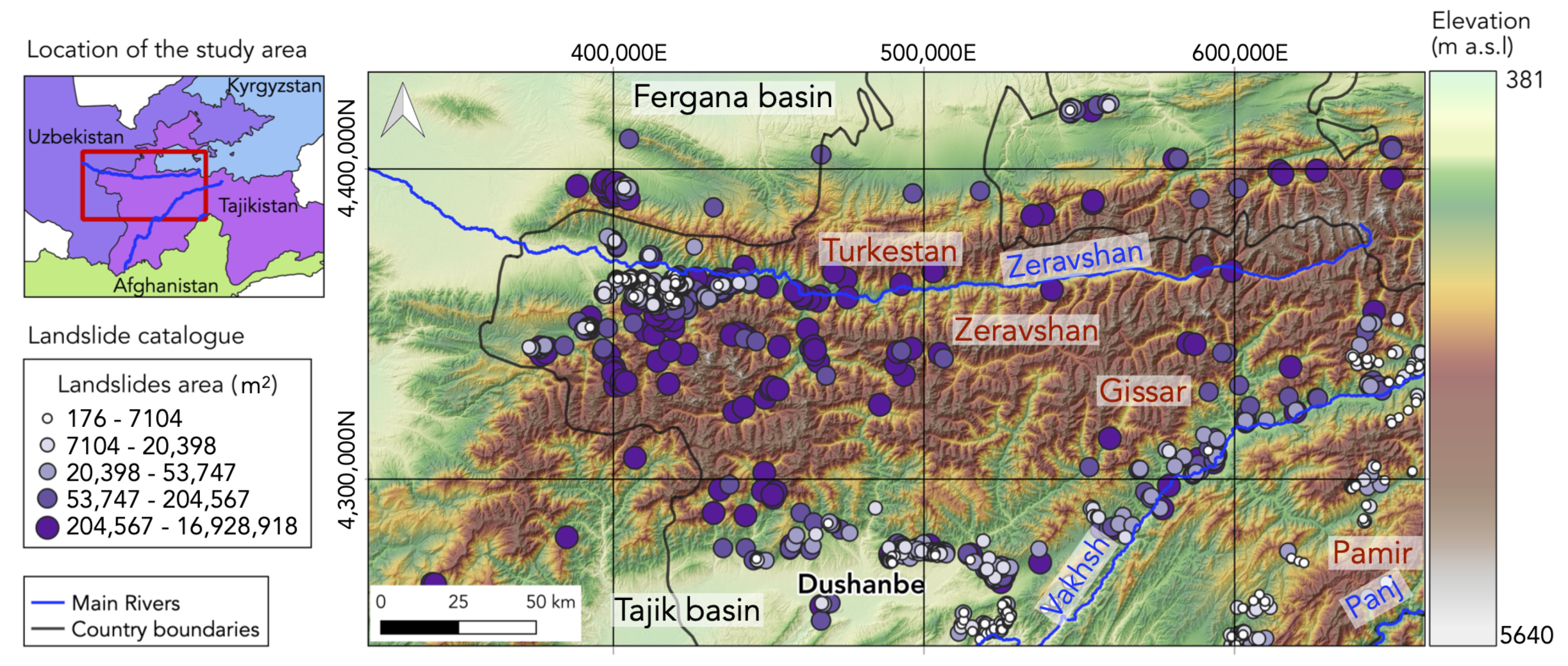
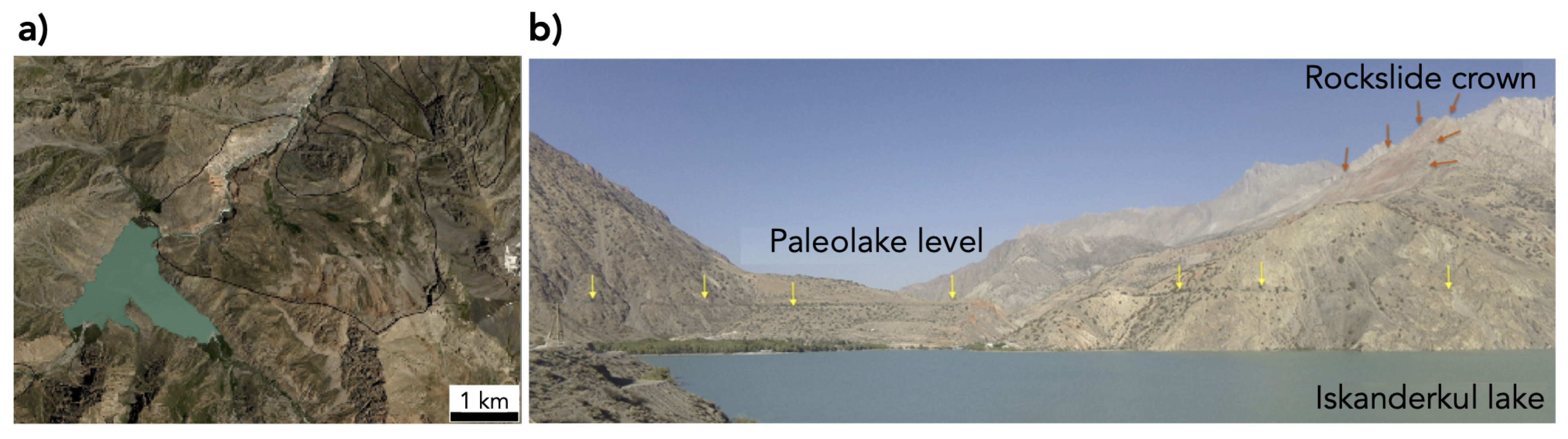
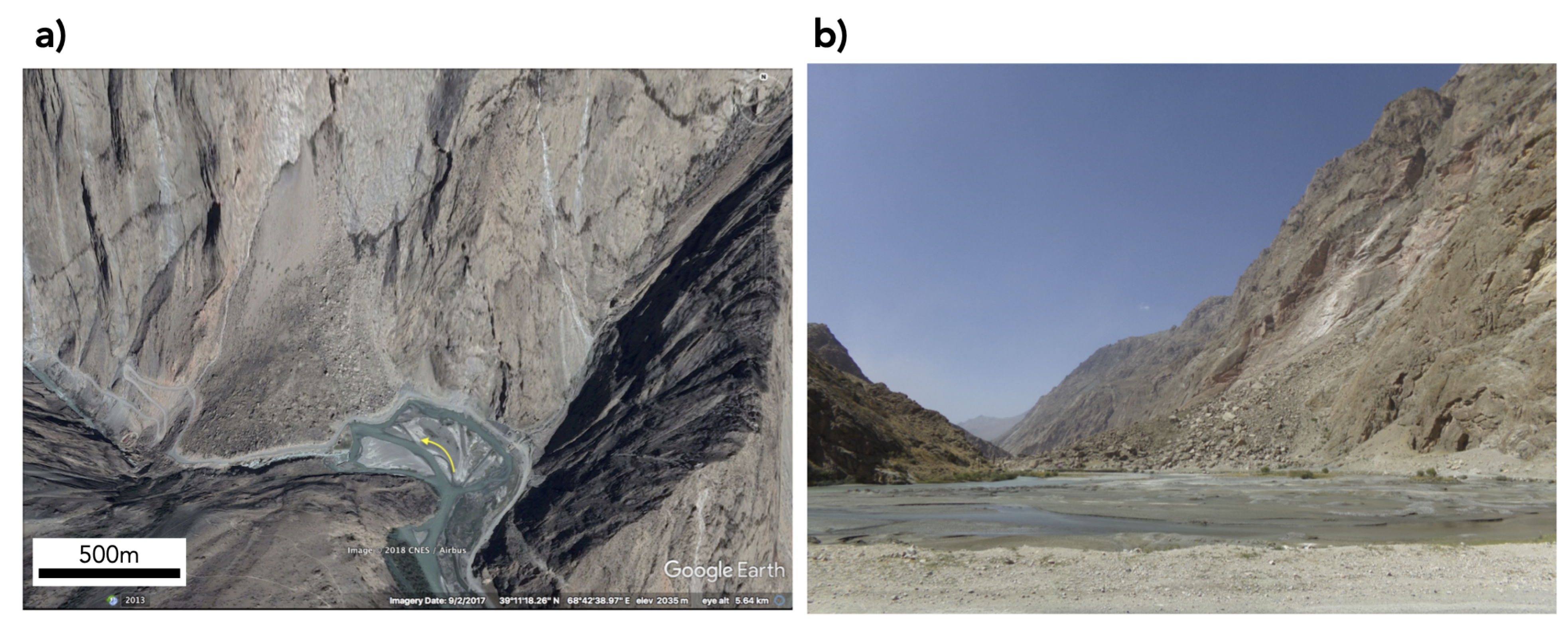
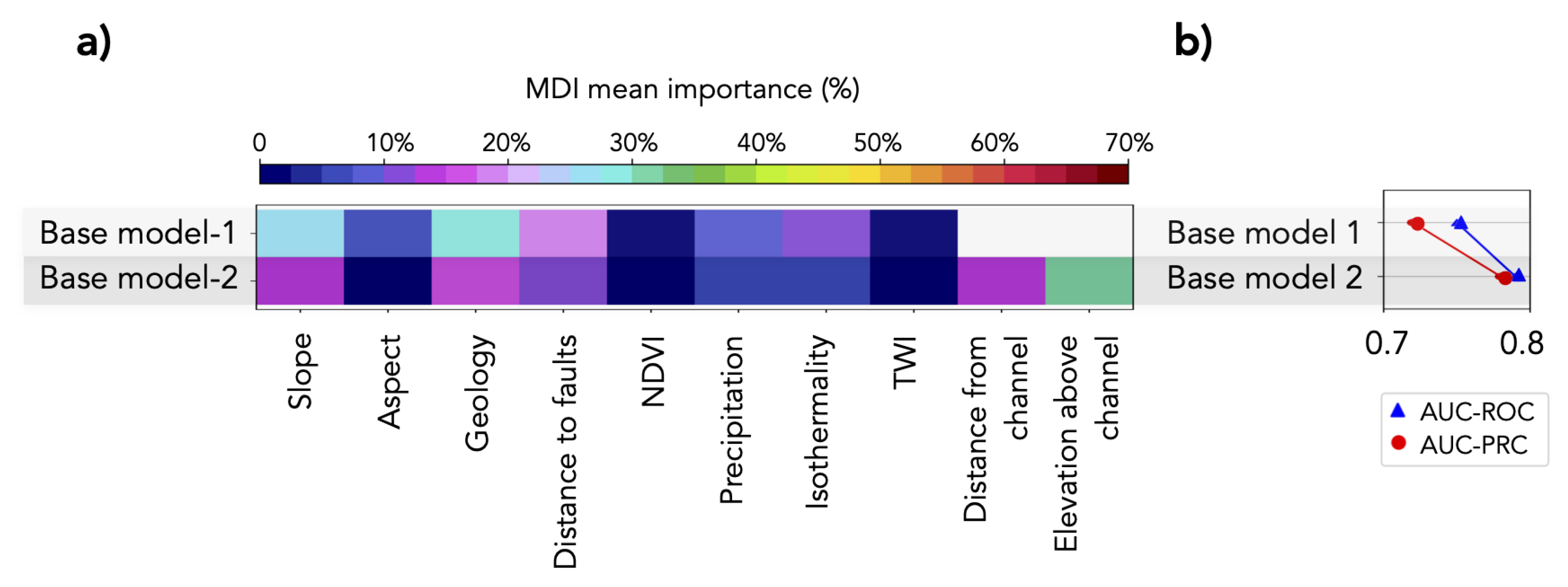
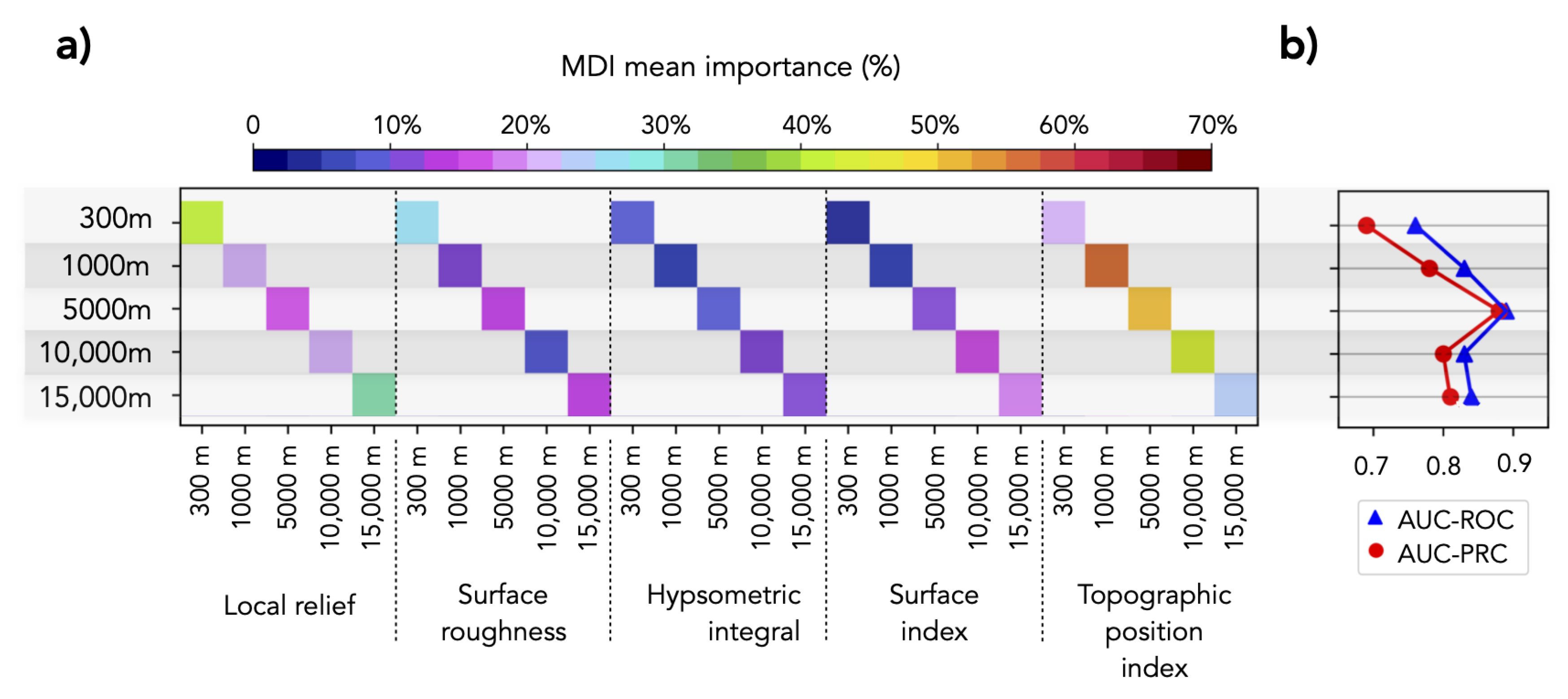
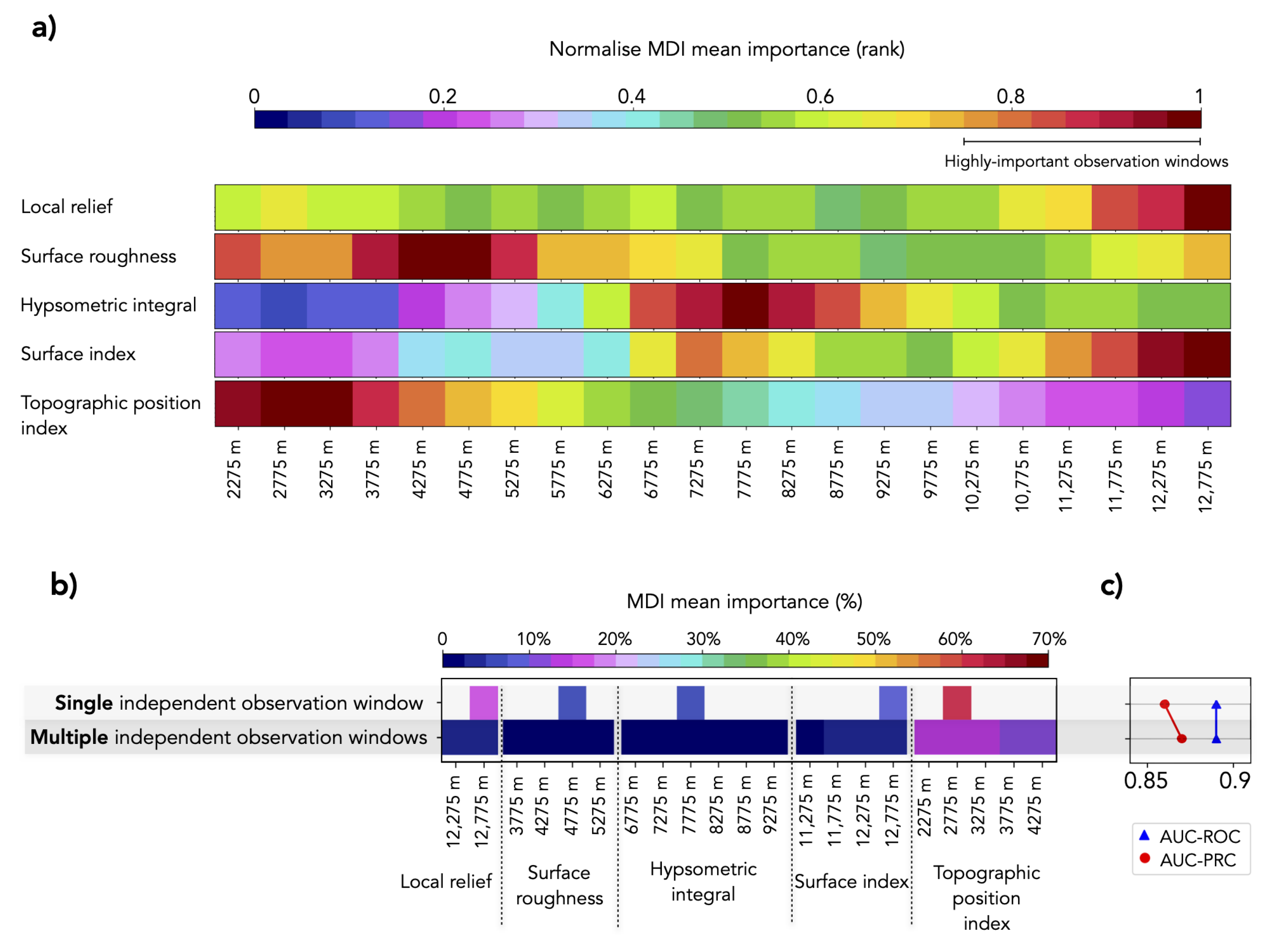
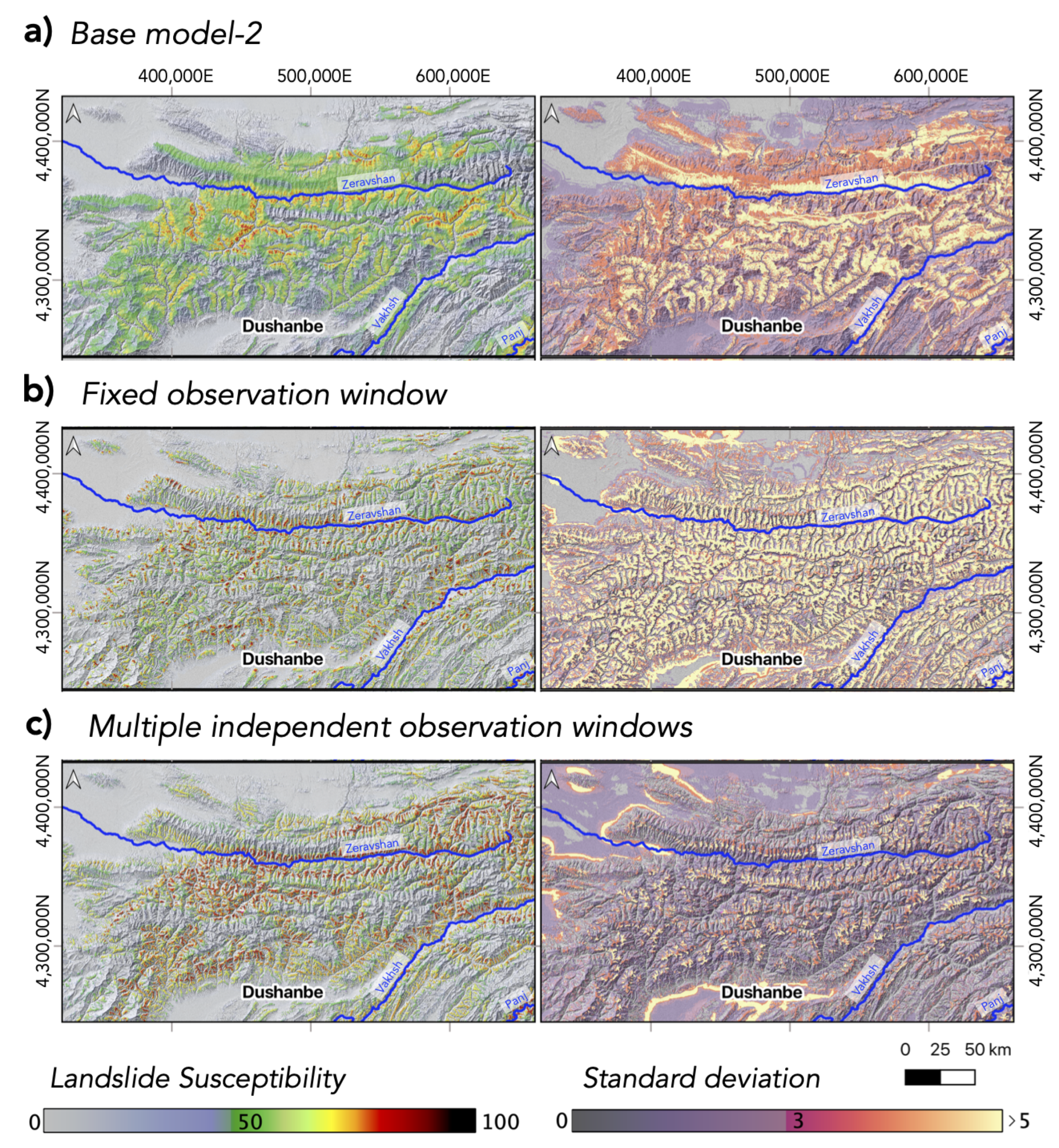
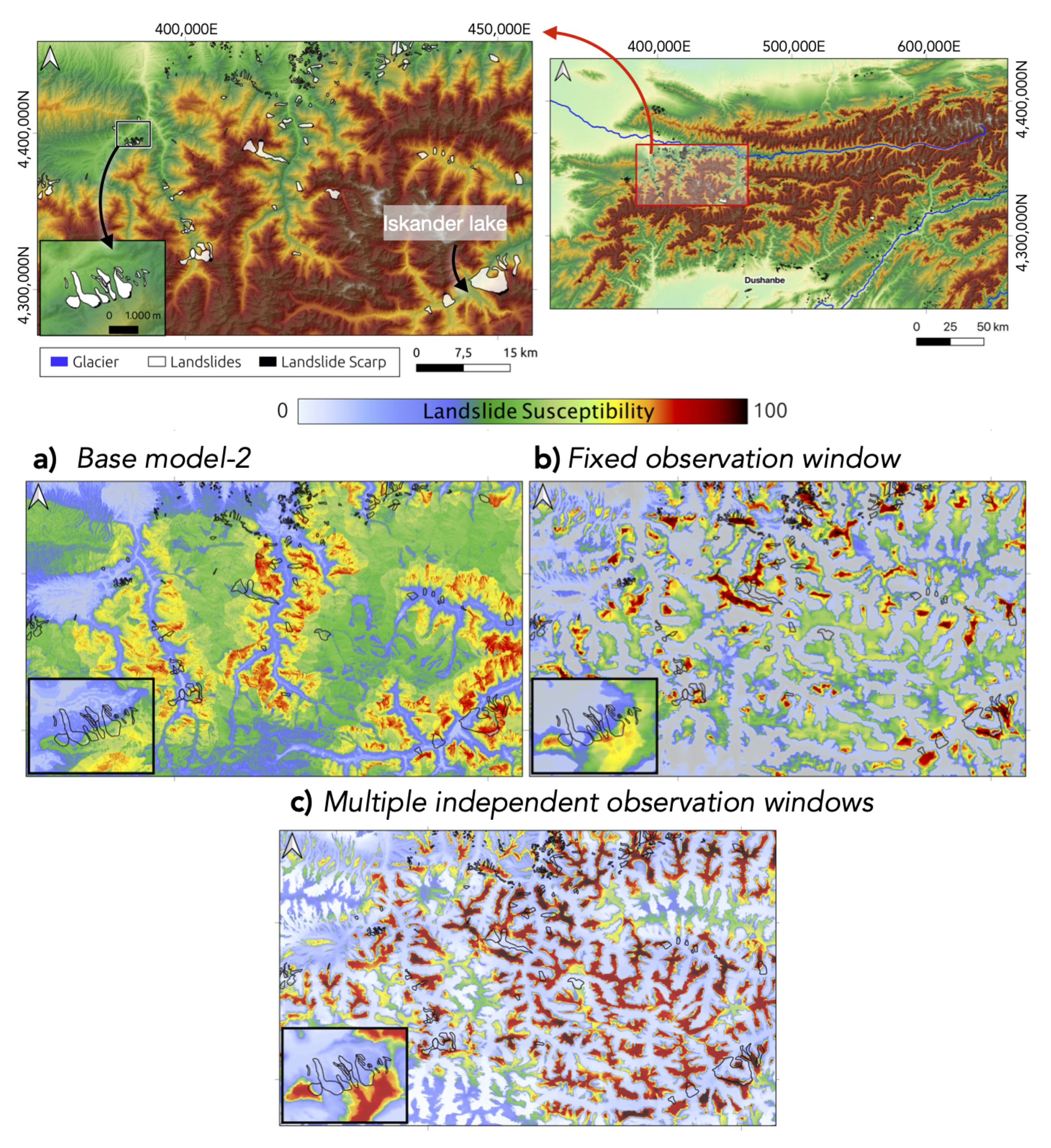
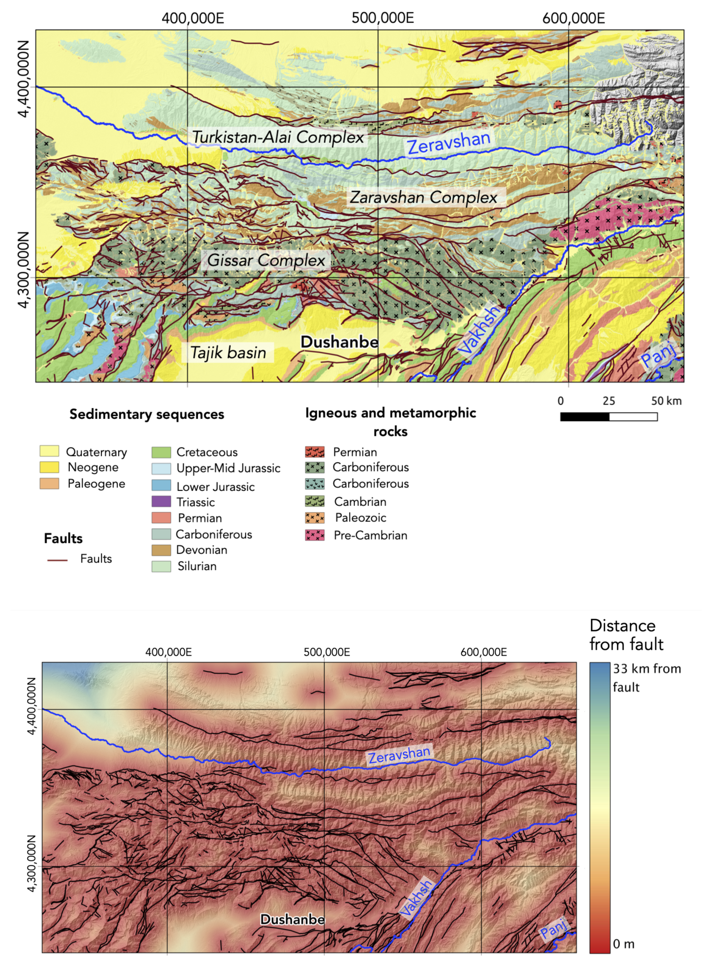
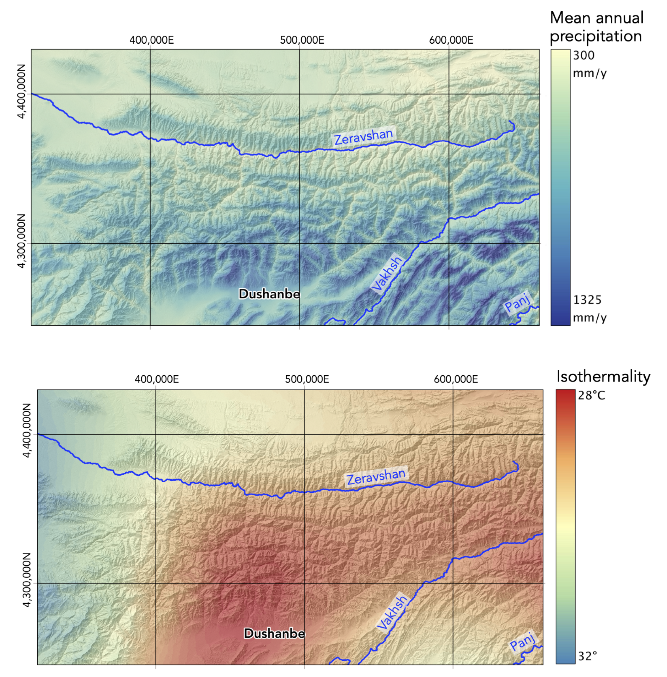
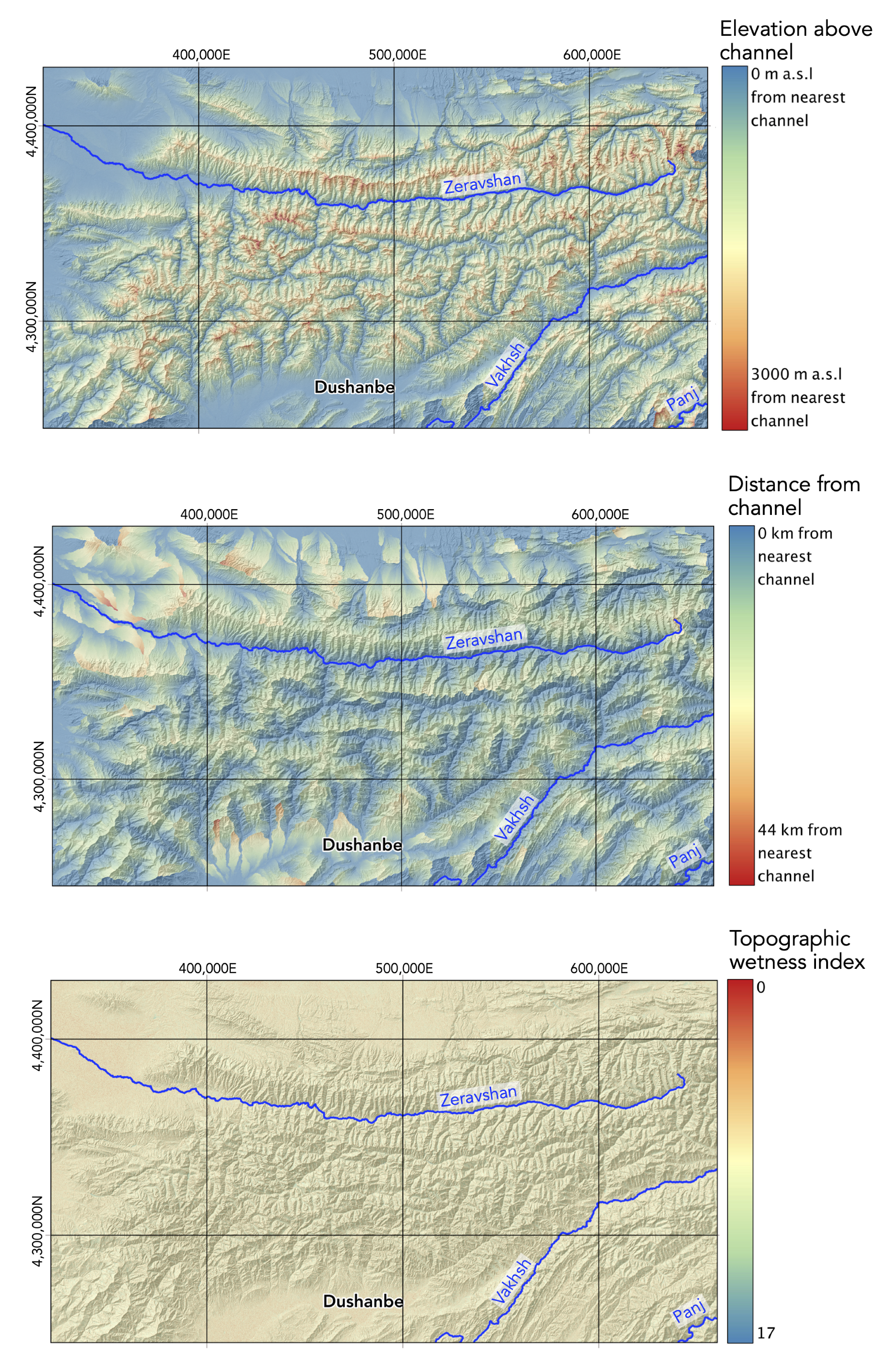
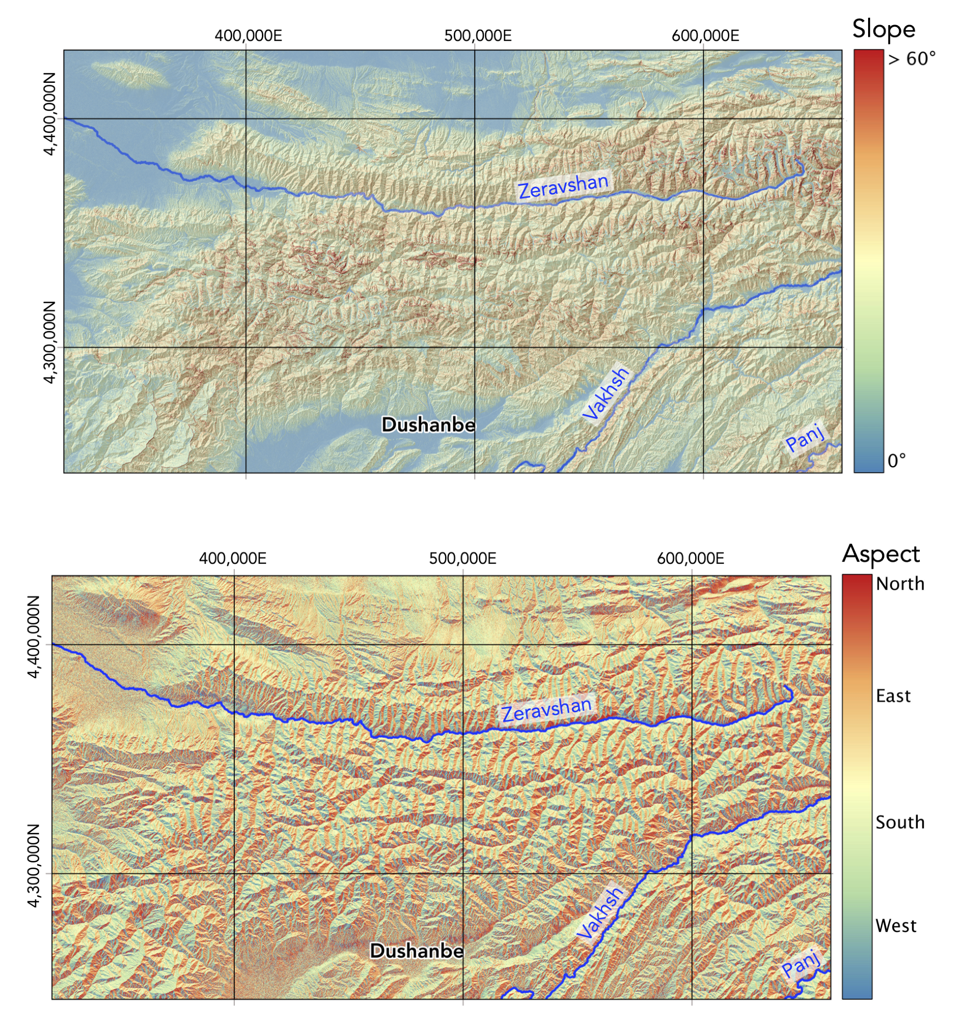
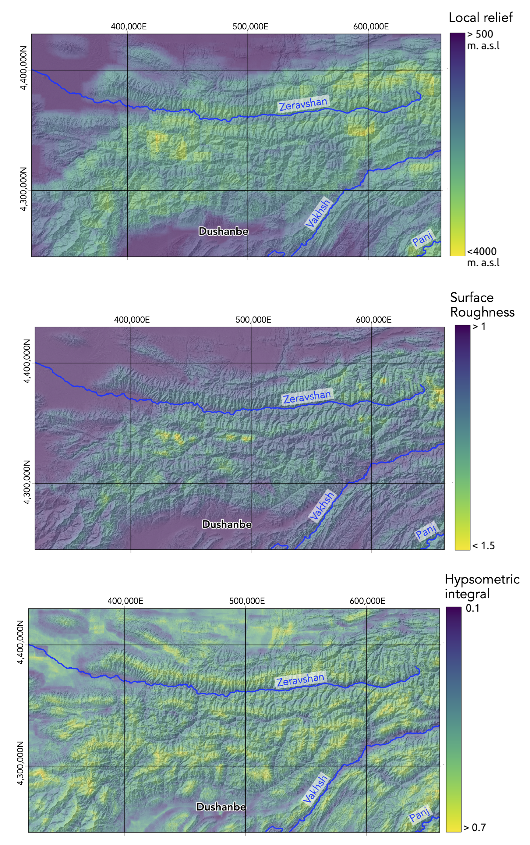
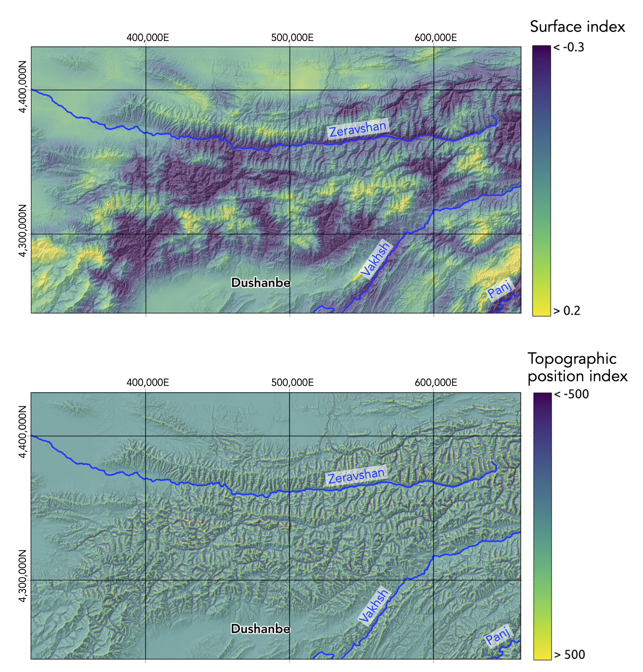
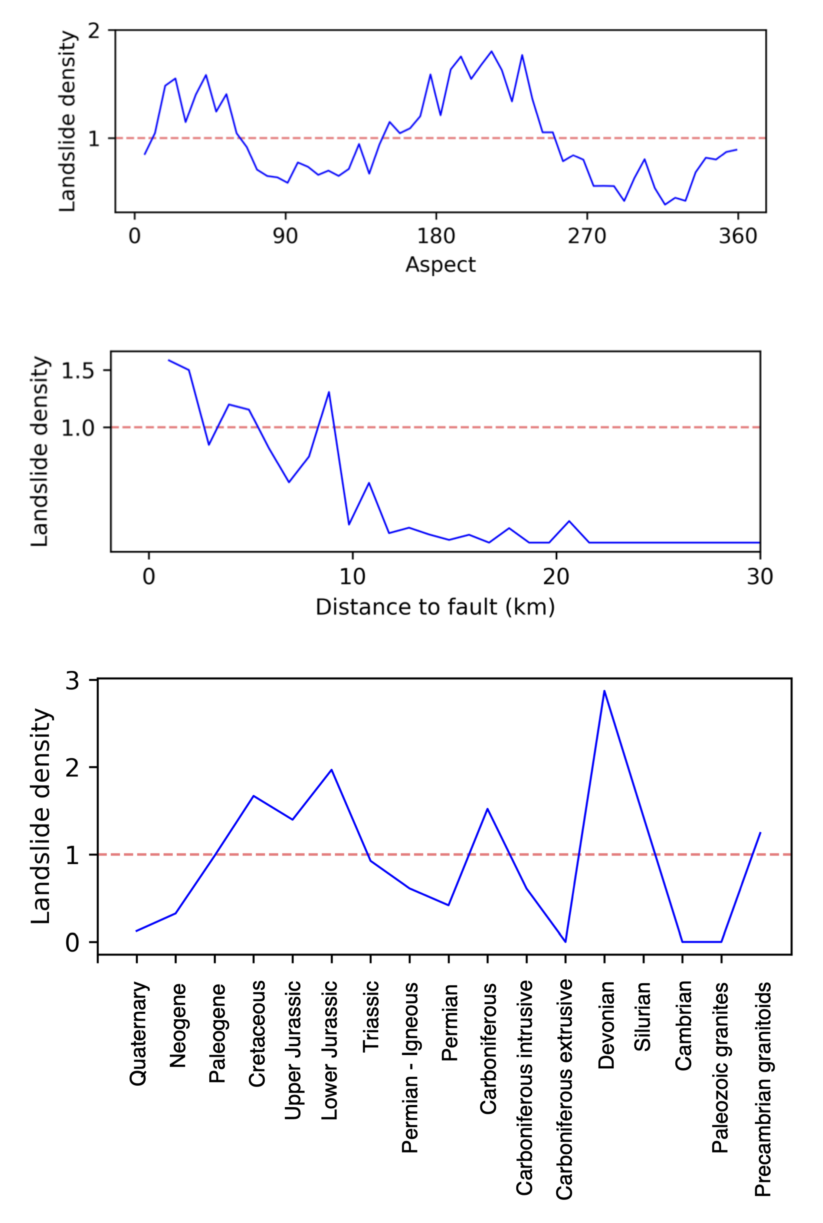
Table 1.
Random forest hyperparameter tuning.
| Hyperparameter | Definition |
|---|---|
| max_features | Number of features considered for splitting a node. |
| min_sample_split | Minimum number of observations in any given node in order to split the node. |
| min_sample_leaf | Minimum number of samples that should be present in the leaf node after splitting a node. |
Table 2.
Datasets and interpreted relevance.
| Thematic Group | Predictive Variable | Significance |
|---|---|---|
| Geology | Geology | Rock type association |
| Distance to fault | Effects of seismicity and fragility on surface materials | |
| Climatic | Mean annual precipitation | Soil saturation and rainfall trigger |
| Isothermality | Seasonal temperature influence on rock fragility and snow melting | |
| Landcover | Normalized Difference vegetation index | Slope instabilities in relation to presence or absence of vegetation |
| Hydrology | Elevation above channel | Influence of gradient and potential energy |
| Distance to channel | Influence of river erosion and deposition | |
| Topographic wetness index | Potential saturation | |
| Geomorphology | Slope | Potential energy to mobilize material |
| Aspect | Effects of sun/wind exposition and favorable surfaces for sliding | |
| Local relief | River incision | |
| Topographic position index | Separation of ridges, valley bottoms, and flats | |
| Surface roughness | Erosion | |
| Hypsometric integral | Characterization of degree of landscape erosion and geomorphological evolution | |
| Surface Index | Discrimination between erosional and steady-state landscapes |
Publisher’s Note: MDPI stays neutral with regard to jurisdictional claims in published maps and institutional affiliations. |
© 2021 by the authors. Licensee MDPI, Basel, Switzerland. This article is an open access article distributed under the terms and conditions of the Creative Commons Attribution (CC BY) license (http://creativecommons.org/licenses/by/4.0/).
Share and Cite
MDPI and ACS Style
Barbosa, N.; Andreani, L.; Gloaguen, R.; Ratschbacher, L. Window-Based Morphometric Indices as Predictive Variables for Landslide Susceptibility Models. Remote Sens. 2021, 13, 451. https://doi.org/10.3390/rs13030451
AMA Style
Barbosa N, Andreani L, Gloaguen R, Ratschbacher L. Window-Based Morphometric Indices as Predictive Variables for Landslide Susceptibility Models. Remote Sensing. 2021; 13(3):451. https://doi.org/10.3390/rs13030451
Chicago/Turabian StyleBarbosa, Natalie, Louis Andreani, Richard Gloaguen, and Lothar Ratschbacher. 2021. "Window-Based Morphometric Indices as Predictive Variables for Landslide Susceptibility Models" Remote Sensing 13, no. 3: 451. https://doi.org/10.3390/rs13030451
Note that from the first issue of 2016, this journal uses article numbers instead of page numbers. See further details here.