
A Regional Maize Yield Hierarchical Linear Model Combining Landsat 8 Vegetative Indices and Meteorological Data: Case Study in Jilin Province


Abstract
:
1. Introduction
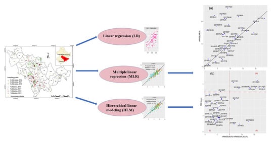
2. Methods
3. Materials
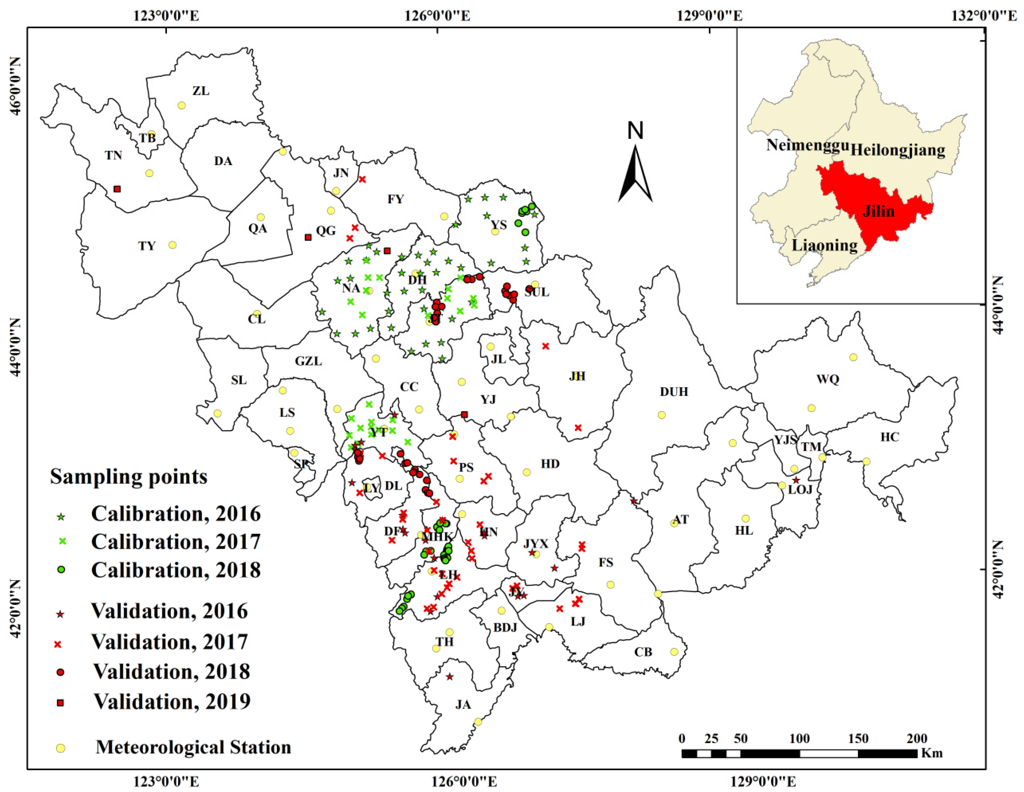
3.1. Study Area
3.2. Remote Sensing Data
3.3. Climatic Data
3.4. Yield Measurement
3.5. Statistical Analysis
4. Result
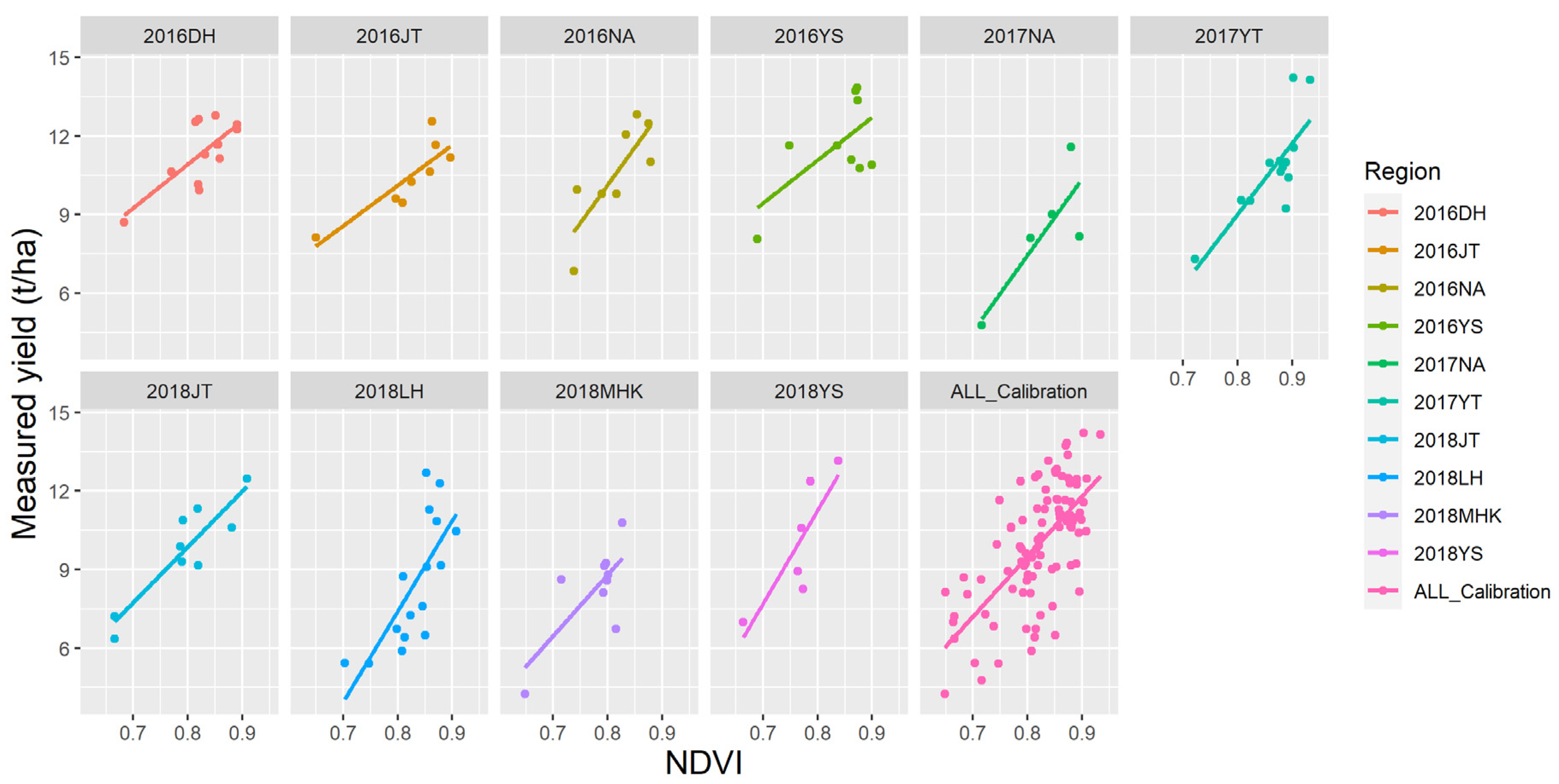
4.1. Correlations between Yield and Spectral Vegetation Indices
4.2. Yield-Predicting Model Combining Landsat 8 Vegetative Indices and Meteorological Data
4.2.1. HLM
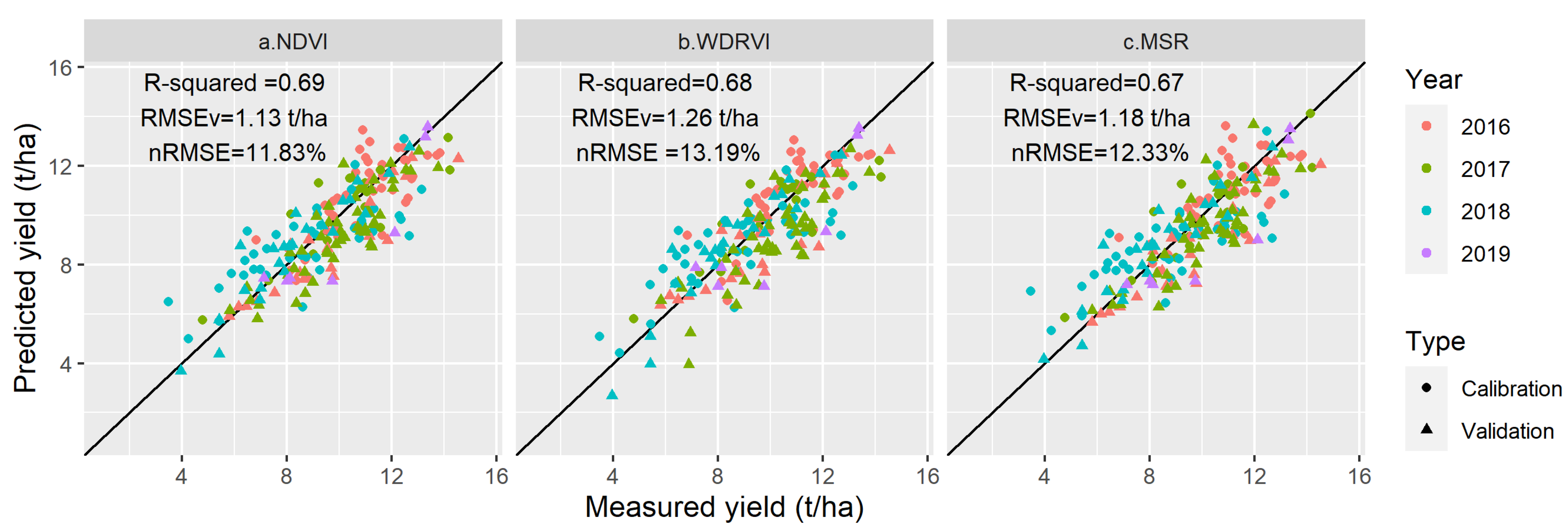
4.2.2. MLR Model
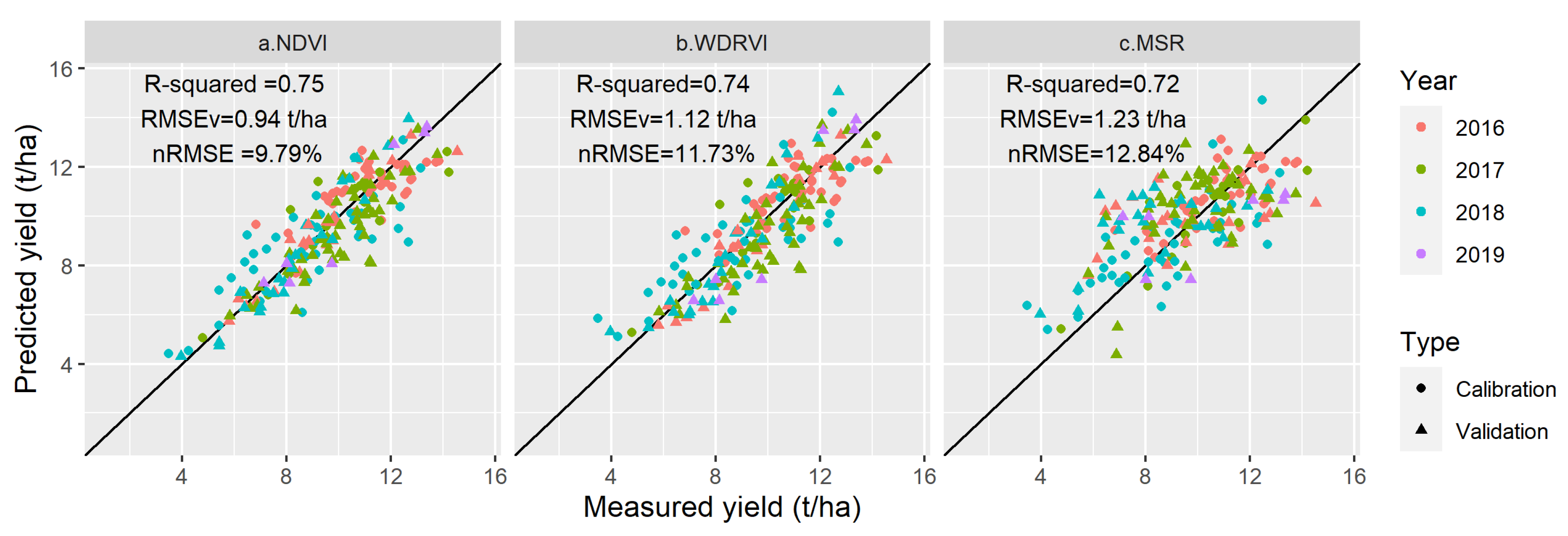
4.3. Evaluation of HLM Method for Yield Prediction
4.3.1. Accuracy Comparison between LR, MLR, and HLM
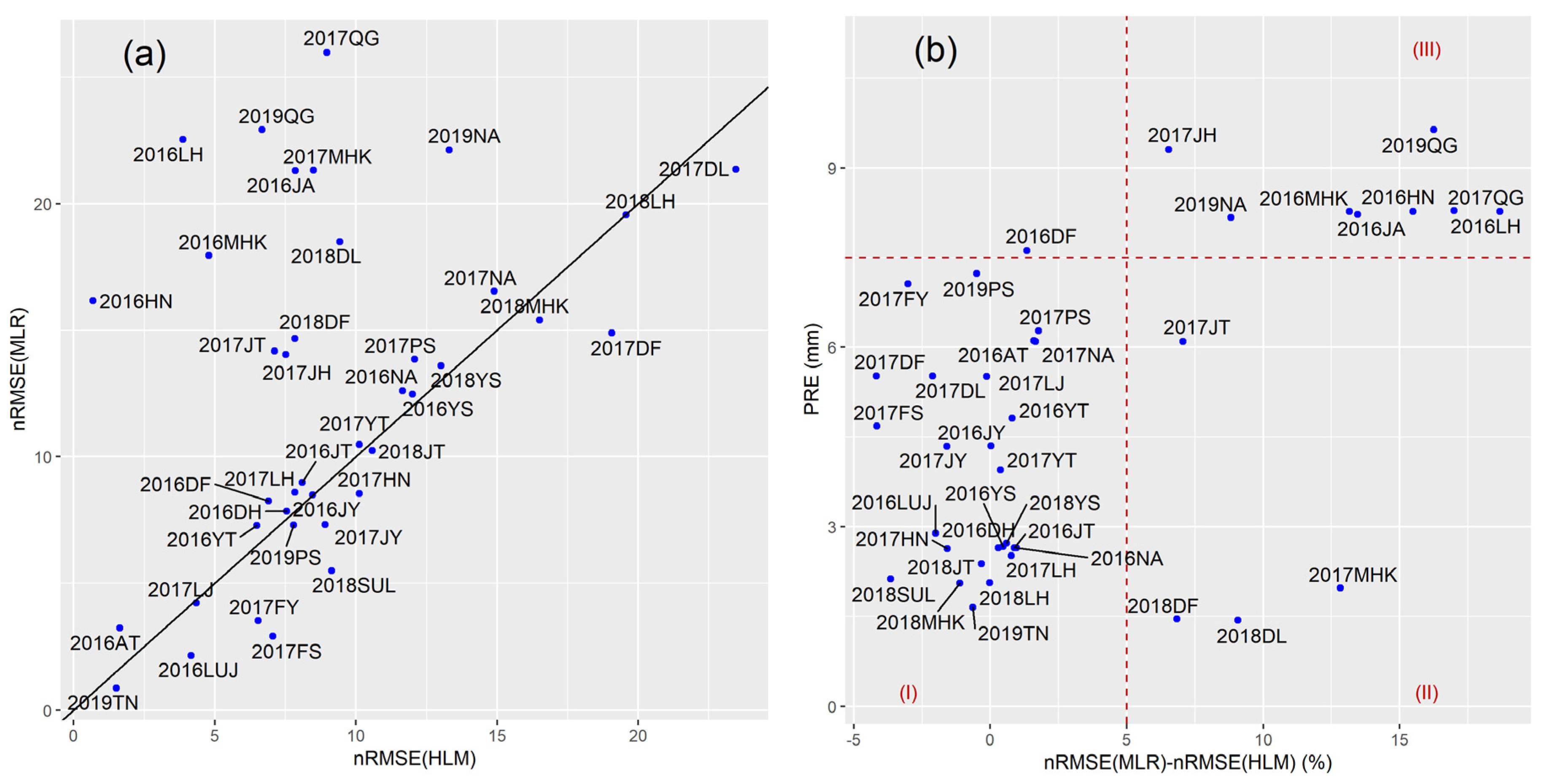
4.3.2. Accuracy Comparison of HLM and MLR Methods in Different Regions
5. Discussion
5.1. Predicting Yield Model
5.2. Potential and Limitations for Yield Prediction
6. Conclusions
Author Contributions
Funding
Institutional Review Board Statement
Informed Consent Statement
Data Availability Statement
Conflicts of Interest
References
- Weiss, M.; Jacob, F.; Duveiller, G. Remote sensing for agricultural applications: A meta-review. Remote Sens. Environ. 2020, 236, 111402. [Google Scholar] [CrossRef]
- Kantanantha, N.; Serban, N.; Griffin, P. Yield and price forecasting for stochastic crop decision planning. J. Agric. Biol. Environ. Stat. 2010, 15, 362–380. [Google Scholar] [CrossRef]
- Stone, R.C.; Meinke, H. Operational seasonal forecasting of crop performance. Philos. Trans. R. Soc. B Biol. Sci. 2005, 360, 2109–2124. [Google Scholar] [CrossRef] [Green Version]
- Córdoba, M.A.; Bruno, C.I.; Costa, J.L.; Peralta, N.R.; Balzarini, M.G. Protocol for multivariate homogeneous zone delineation in precision agriculture. Biosyst. Eng. 2016, 143, 95–107. [Google Scholar] [CrossRef]
- Cui, B.; Zhao, Q.; Huang, W.; Song, X.; Ye, H.; Zhou, X. A new integrated vegetation index for the estimation of winter wheat leaf chlorophyll content. Remote Sens. 2019, 11, 974. [Google Scholar] [CrossRef] [Green Version]
- Ciampitti, I.A.; Vyn, T.J. Grain nitrogen source changes over time in maize: A review. Crop Sci. 2013, 53, 366–377. [Google Scholar] [CrossRef] [Green Version]
- Meng, Q.; Cui, Z.; Yang, H.; Zhang, F.; Chen, X. Establishing High-Yielding Maize System for Sustainable Intensification in China, 1st ed.; Elsevier Inc.: Amsterdam, The Netherlands, 2018; Volume 148, ISBN 9780128151792. [Google Scholar]
- Silva, P.R.F.D.; Strieder, M.L.; Coser, R.P.D.S.; Rambo, L.; Sangoi, L.; Argenta, G.; Forsthofer, E.L.; Silva, A.A.D. Grain yield and kernel crude protein content increases of maize hybrids with late nitrogen side-dressing. Sci. Agric. 2005, 62, 487–492. [Google Scholar] [CrossRef] [Green Version]
- Filippi, P.; Jones, E.J.; Wimalathunge, N.S.; Somarathna, P.D.S.N.; Pozza, L.E.; Ugbaje, S.U.; Jephcott, T.G.; Paterson, S.E.; Whelan, B.M.; Bishop, T.F.A. An approach to forecast grain crop yield using multi-layered, multi-farm data sets and machine learning. Precis. Agric. 2019, 20, 1015–1029. [Google Scholar] [CrossRef]
- Kogan, F.; Guo, W.; Yang, W. Drought and food security prediction from NOAA new generation of operational satellites. Geomat. Nat. Hazards Risk 2019, 10, 651–666. [Google Scholar] [CrossRef] [Green Version]
- Battude, M.; Al Bitar, A.; Morin, D.; Cros, J.; Huc, M.; Marais Sicre, C.; Le Dantec, V.; Demarez, V. Estimating maize biomass and yield over large areas using high spatial and temporal resolution Sentinel-2 like remote sensing data. Remote Sens. Environ. 2016, 184, 668–681. [Google Scholar] [CrossRef]
- Lobell, D.B.; Asner, G.P.; Ortiz-Monasterio, J.I.; Benning, T.L. Remote sensing of regional crop production in the Yaqui Valley, Mexico: Estimates and uncertainties. Agric. Ecosyst. Environ. 2003, 94, 205–220. [Google Scholar] [CrossRef] [Green Version]
- Karthikeyan, L.; Chawla, I.; Mishra, A.K. A review of remote sensing applications in agriculture for food security: Crop growth and yield, irrigation, and crop losses. J. Hydrol. 2020, 586, 124905. [Google Scholar] [CrossRef]
- Corti, M.; Cavalli, D.; Cabassi, G.; Marino Gallina, P.; Bechini, L. Does remote and proximal optical sensing successfully estimate maize variables? A review. Eur. J. Agron. 2018, 99, 37–50. [Google Scholar] [CrossRef]
- Li, Z.; Wang, J.; Xu, X.; Zhao, C.; Jin, X.; Yang, G.; Feng, H. Assimilation of two variables derived from hyperspectral data into the DSSAT-CERES model for grain yield and quality estimation. Remote Sens. 2015, 7, 12400–12418. [Google Scholar] [CrossRef] [Green Version]
- Ban, H.Y.; Ahn, J.B.; Lee, B.W. Assimilating MODIS data-derived minimum input data set and water stress factors into CERES-Maize model improves regional corn yield predictions. PLoS ONE 2019, 14, 1–21. [Google Scholar] [CrossRef]
- Jin, X.; Li, Z.; Feng, H.; Ren, Z.; Li, S. Estimation of maize yield by assimilating biomass and canopy cover derived from hyperspectral data into the AquaCrop model. Agric. Water Manag. 2020, 227, 105846. [Google Scholar] [CrossRef]
- Jin, X.; Kumar, L.; Li, Z.; Feng, H.; Xu, X.; Yang, G.; Wang, J. A review of data assimilation of remote sensing and crop models. Eur. J. Agron. 2018, 92, 141–152. [Google Scholar] [CrossRef]
- Dorigo, W.A.; Zurita-Milla, R.; de Wit, A.J.W.; Brazile, J.; Singh, R.; Schaepman, M.E. A review on reflective remote sensing and data assimilation techniques for enhanced agroecosystem modeling. Int. J. Appl. Earth Obs. Geoinf. 2007, 9, 165–193. [Google Scholar] [CrossRef]
- Zhou, X.; Zheng, H.B.; Xu, X.Q.; He, J.Y.; Ge, X.K.; Yao, X.; Cheng, T.; Zhu, Y.; Cao, W.X.; Tian, Y.C. Predicting grain yield in rice using multi-temporal vegetation indices from UAV-based multispectral and digital imagery. ISPRS J. Photogramm. Remote Sens. 2017, 130, 246–255. [Google Scholar] [CrossRef]
- Ramos, A.P.M.; Osco, L.P.; Furuya, D.E.G.; Gonçalves, W.N.; Santana, D.C.; Teodoro, L.P.R.; da Silva Junior, C.A.; Capristo-Silva, G.F.; Li, J.; Baio, F.H.R.; et al. A random forest ranking approach to predict yield in maize with uav-based vegetation spectral indices. Comput. Electron. Agric. 2020, 178, 105791. [Google Scholar] [CrossRef]
- Johnson, M.D.; Hsieh, W.W.; Cannon, A.J.; Davidson, A.; Bédard, F. Crop yield forecasting on the Canadian Prairies by remotely sensed vegetation indices and machine learning methods. Agric. For. Meteorol. 2016, 218–219, 74–84. [Google Scholar] [CrossRef]
- Alganci, U.; Ozdogan, M.; Sertel, E.; Ormeci, C. Estimating maize and cotton yield in southeastern Turkey with integrated use of satellite images, meteorological data and digital photographs. F. Crop. Res. 2014, 157, 8–19. [Google Scholar] [CrossRef]
- Balaghi, R.; Tychon, B.; Eerens, H.; Jlibene, M. Empirical regression models using NDVI, rainfall and temperature data for the early prediction of wheat grain yields in Morocco. Int. J. Appl. Earth Obs. Geoinf. 2008, 10, 438–452. [Google Scholar] [CrossRef] [Green Version]
- Aghighi, H.; Azadbakht, M.; Ashourloo, D.; Shahrabi, H.S.; Radiom, S. Machine Learning Regression Techniques for the Silage Maize Yield Prediction Using Time-Series Images of Landsat 8 OLI. IEEE J. Sel. Top. Appl. Earth Obs. Remote Sens. 2018, 11, 4563–4577. [Google Scholar] [CrossRef]
- Chlingaryan, A.; Sukkarieh, S.; Whelan, B. Machine learning approaches for crop yield prediction and nitrogen status estimation in precision agriculture: A review. Comput. Electron. Agric. 2018, 151, 61–69. [Google Scholar] [CrossRef]
- Singh, R.P.; Roy, S.; Kogan, F. Vegetation and temperature condition indices from NOAA AVHRR data for drought monitoring over India. Int. J. Remote Sens. 2003, 24, 4393–4402. [Google Scholar] [CrossRef]
- Piedallu, C.; Chéret, V.; Denux, J.P.; Perez, V.; Azcona, J.S.; Seynave, I.; Gégout, J.C. Soil and climate differently impact NDVI patterns according to the season and the stand type. Sci. Total Environ. 2019, 651, 2874–2885. [Google Scholar] [CrossRef]
- Li, Z.; Taylor, J.; Yang, H.; Casa, R.; Jin, X.; Li, Z.; Song, X.; Yang, G. A hierarchical interannual wheat yield and grain protein prediction model using spectral vegetative indices and meteorological data. Field Crop. Res. 2020, 248, 107711. [Google Scholar] [CrossRef]
- Osborne, J.; Osborne, J.W. A Brief Introduction to Hierarchical Linear Modeling. Best Pract. Quant. Methods 2011, 8, 444–450. [Google Scholar]
- Gavin, M.B.; Hofmann, D.A. Using hierarchical linear modeling to investigate the moderating influence of leardership climate. Leadersh. Q. 2002, 13, 15–33. [Google Scholar] [CrossRef]
- Bock, R.D. Multilevel Analysis of Educational Data; Academic Press, Inc.: London, UK, 1989. [Google Scholar]
- Banerjee, S.; Carlin, B.P.; Gelfand, A.E. Hierarchical Modeling and Analysis for Spatial Data, 2nd ed.; Taylor & Francis: Abingdon, UK, 2015. [Google Scholar]
- Butts-Wilmsmeyer, C.J.; Seebauer, J.R.; Singleton, L.; Below, F.E. Weather during key growth stages explains grain quality and yield of maize. Agronomy 2019, 9, 16. [Google Scholar] [CrossRef] [Green Version]
- Vollmer, E.; Mußhoff, O. Average protein content and its variability in winter wheat: A forecast model based on weather parameters. Earth Interact. 2018, 22, 1–24. [Google Scholar] [CrossRef]
- Lee, B.H.; Kenkel, P.; Brorsen, B.W. Pre-harvest forecasting of county wheat yield and wheat quality using weather information. Agric. For. Meteorol. 2013, 168, 26–35. [Google Scholar] [CrossRef]
- Guo, E.; Zhang, J.; Wang, Y.; Si, H.; Zhang, F. Dynamic risk assessment of waterlogging disaster for maize based on CERES-Maize model in Midwest of Jilin Province, China. Nat. Hazards 2016, 83, 1747–1761. [Google Scholar] [CrossRef]
- Wang, M.; Li, Y.; Ye, W.; Bornman, J.F.; Yan, X. Effects of climate change on maize production, and potential adaptation measures: A case study in Jilin province, China. Clim. Res. 2011, 46, 223–242. [Google Scholar] [CrossRef] [Green Version]
- Zhu, Z.; Wang, S.; Woodcock, C.E. Improvement and expansion of the Fmask algorithm: Cloud, cloud shadow, and snow detection for Landsats 4-7, 8, and Sentinel 2 images. Remote Sens. Environ. 2015, 159, 269–277. [Google Scholar] [CrossRef]
- Zarco-Tejada, P.J.; Berjón, A.; López-Lozano, R.; Miller, J.R.; Martín, P.; Cachorro, V.; González, M.R.; De Frutos, A. Assessing vineyard condition with hyperspectral indices: Leaf and canopy reflectance simulation in a row-structured discontinuous canopy. Remote Sens. Environ. 2005, 99, 271–287. [Google Scholar] [CrossRef]
- Chen, J.M. Evaluation of vegetation indices and a modified simple ratio for boreal applications. Can. J. Remote Sens. 1996, 22, 229–242. [Google Scholar] [CrossRef]
- Gitelson, A.A.; Kaufman, Y.J.; Merzlyak, M.N. Use of a green channel in remote sensing of global vegetation from EOS- MODIS. Remote Sens. Environ. 1996, 58, 289–298. [Google Scholar] [CrossRef]
- Vincini, M.; Frazzi, E. Angular dependence of maize and sugar beet VIs from directional CHRIS/Proba data. In Proceedings of the 4th ESA CHRIS PROBA Workshop, Frascati, Italy, 19–21 September 2006; Volume 2006, pp. 19–21. [Google Scholar]
- Jordan, C.F. Derivation of leaf-area index from qualityof light on the forest floor. Ecol. Soc. Am. 1969, 50, 663–666. [Google Scholar]
- Sripada, R.P.; Heiniger, R.W.; White, J.G.; Weisz, R. Aerial color infrared photography for determining late-season nitrogen requirements in corn. Agron. J. 2005, 97, 1443–1451. [Google Scholar] [CrossRef]
- Huete, A.R. A soil-adjusted vegetation index (SAVI). Remote Sens. Environ. 1988, 25, 295–309. [Google Scholar] [CrossRef]
- Broge, N.H.; Leblanc, E. Comparing prediction power and stability of broadband and hyperspectral vegetation indices for estimation of green leaf area index and canopy chlorophyll density. Remote Sens. Environ. 2001, 76, 156–172. [Google Scholar] [CrossRef]
- Wu, C.; Wang, L.; Niu, Z.; Gao, S.; Wu, M. Nondestructive estimation of canopy chlorophyll content using Hyperion and Landsat/TM images. Int. J. Remote Sens. 2010, 31, 2159–2167. [Google Scholar] [CrossRef]
- Gitelson, A.A. Wide Dynamic Range Vegetation Index for Remote Quantification of Biophysical Characteristics of Vegetation. J. Plant Physiol. 2004, 161, 165–173. [Google Scholar] [CrossRef] [Green Version]
- Bozdogan, H. Model selection and Akaike’s Information Criterion (AIC): The general theory and its analytical extensions. Psychometrika 1987, 52, 345–370. [Google Scholar] [CrossRef]
- Kuznetsova, A.; Brockhoff, P.B.; Christensen, R.H.B. lmerTest Package: Tests in Linear Mixed Effects Models. J. Stat. Softw. 2017, 82, 1–26. [Google Scholar] [CrossRef] [Green Version]
- Wickham, H. Ggplot2: Elegant Graphics for Data Analysis; Springer-Verlag: New York, NY, USA, 2016; ISBN 978-3-319-24277-4. [Google Scholar]
- Cociu, A.I.; Alionte, E. Effect of Different Tillage Systems on Grain Yield and Its Quality of Winter Wheat, Maize and Soybean under Different Weather Conditions. Rom. Agric. Res. 2017, 34, 59–67. [Google Scholar]
- Prasad, A.K.; Chai, L.; Singh, R.P.; Kafatos, M. Crop yield estimation model for Iowa using remote sensing and surface parameters. Int. J. Appl. Earth Obs. Geoinf. 2006, 8, 26–33. [Google Scholar] [CrossRef]
- Araya, S.; Ostendorf, B.; Lyle, G.; Lewis, M. CropPhenology: An R package for extracting crop phenology from time series remotely sensed vegetation index imagery. Ecol. Inform. 2018, 46, 45–56. [Google Scholar] [CrossRef]
- Nissanka, S.P.; Karunaratne, A.S.; Perera, R.; Weerakoon, W.M.W.; Thorburn, P.J.; Wallach, D. Calibration of the phenology sub-model of APSIM-Oryza: Going beyond goodness of fit. Environ. Model. Softw. 2015, 70, 128–137. [Google Scholar] [CrossRef]
- Ramoelo, A.; Cho, M.; Mathieu, R.; Skidmore, A.K. The potential of Sentinel-2 spectral configuration to assess rangeland quality. Remote Sens. Agric. Ecosyst. Hydrol. XVI 2014, 9239, 92390C. [Google Scholar] [CrossRef] [Green Version]
- Magney, T.S.; Eitel, J.U.H.; Vierling, L.A. Mapping wheat nitrogen uptake from RapidEye vegetation indices. Precis. Agric. 2017, 18, 429–451. [Google Scholar] [CrossRef]


| Date | Scene ID | Path | Row | Sampling Areas and Grain-Filling Date |
|---|---|---|---|---|
| 14 August 2016 | LC81170302016227LGN01 | 117 | 30 | 2016AT (7 August 2016) |
| 14 August 2016 | LC81170312016227LGN01 | 117 | 31 | 2016JY (8/12/2016) 2016JA (12 August 2016) 2016LH (10 August 2016) 2016MHK (9 August 2016) 2016HN (7 August 2016) |
| 23 August 2016 | LC81150302016229LGN02 | 115 | 30 | 2016LUJ (21 August 2016) |
| 5 August 2016 | LC81180302016218LGN01 | 118 | 30 | 2016DF (30 July 2016) 2016YT (31 July 2016) |
| 5 August 2016 | LC81180292016218LGN01 | 118 | 29 | 2016DH (31 July 2016) 2016JT (3 August 2016) 2016NA (3 August 2016) 2016YS (2 August 2016) |
| 8 August 2017 | LC81180302017220LGN00 | 118 | 30 | 2017DF (8 August 2017) 2017DL (3 August 2017) 2017HN (8 August 2017) 2017MHK (6 August 2017) 2017PS (8 August 2017) 2017NA (7 August 2017) 2017YT (5 August 2017) 2017LS (5 August 2017) |
| 1 August /2017 | LC81170302017213LGN00 | 117 | 30 | 2017FS (28 July 2017) |
| 8 August 2017 | LC81180292017220LGN00 | 118 | 29 | 2017FY (7 August 2017) 2017QG (4 August 2017) 2017JT (3 August 2017) |
| 17 August 2017 | LC81170302017229LGN00 | 117 | 30 | 2017JH (11 August 2017) |
| 8 August 2017 | LC81180312017220LGN00 | 118 | 31 | 2017LH (8 August 2017) |
| 10 August 2017 | LC81160312017222LGN00 | 116 | 31 | 2017LJ (10 August 2017) |
| 11 August 2018 | LC81180302018223LGN00 | 118 | 30 | 2018DL (7 August 2018) 2018DF (6 August 2018) 2018MHK (10 August 2018) |
| 11 August 2018 | LC81180292018223LGN00 | 118 | 29 | 2018SUL (3 August 2018) 2018JT (3 August 2017) 2017YS (9 August 2018) |
| 11 August 2018 | LC81180312018223LGN00 | 118 | 31 | 2018LH (9 August 2018) |
| 12 August 2019 | LC81200292019224LGN00 | 120 | 29 | 2019TN (7 August 2019) |
| 21 August 2019 | LC81190292019233LGN00 | 119 | 29 | 2019NA (13 August 2019) |
| 29 July 2019 | LC81180302019210LGN00 | 118 | 30 | 2019PS (29 July 2019) |
| 5 August 2019 | LC81190292019217LGN00 | 119 | 29 | 2019QG (5 August 2019) |
| VI | Formula | Correlation | Reference |
|---|---|---|---|
| GI | R551/R677 | 0.491 ** | [40] |
| MSR | (R800/R670 − 1)/sqrt(R800/R670 + 1) | 0.665 ** | [41] |
| NDVI | (R890 − R670)/(R890 + R670) | 0.677 ** | [42] |
| SPVI | 0.4(3.7(R800 − R670) − 1.2abs(R550 − R670)) | 0.447 ** | [43] |
| RVI | NIR/R | 0.634 ** | [44] |
| CInir | NIR/G − 1 | 0.597** | [45] |
| SAVI | (1 + 0.5) (N − R)/(N + R + 0.5) | 0.556 ** | [46] |
| TVI | 0.5[120(NIR − G) − 200(R − G)] | 0.459 ** | [47] |
| EVI | 2.5*(NIR − R)/(NIR + 6*R − 7.5*B + 1) | –0.218 * | [48] |
| EVI2 | 2.5*(NIR − R)/(NIR + 2.4*R + 1) | 0.606 ** | [14] |
| WDRVI | (0.1R890 − R670)/(0.1R890 − R670) | 0.676 ** | [49] |
| Year | 2016 | 2017 | 2018 | 2019 | Total | Calibration | Validation |
|---|---|---|---|---|---|---|---|
| Sample size | 63 | 67 | 64 | 7 | 201 | 100 | 101 |
| Min | 6.15 | 4.78 | 3.47 | 7.13 | 3.47 | 3.47 | 3.95 |
| Mean | 10.46 | 9.97 | 8.64 | 10.25 | 9.71 | 9.86 | 9.56 |
| Max | 14.53 | 14.22 | 13.15 | 13.37 | 14.53 | 14.22 | 14.53 |
| SD | 2.01 | 2.00 | 2.30 | 2.65 | 2.24 | 2.34 | 2.14 |
| CV | 0.19 | 0.20 | 0.27 | 0.26 | 0.23 | 0.24 | 0.22 |
| Region | LR Model | R2 | RMSEV (t/ha) | nRMSE (%) |
|---|---|---|---|---|
| 2016DH | y = –2.43 + 16.68x | 0.53 ** | 2.73 | 28.57 |
| 2016JT | y = –2.25 + 15.45x | 0.73 ** | 2.18 | 22.81 |
| 2016NA | y = –1.81 + 15.41x | 0.59 ** | 2.42 | 25.34 |
| 2016YS | y = –2.02 + 16.38x | 0.40 | 2.84 | 29.72 |
| 2017NA | y = –15.83 + 29.10x | 0.77 * | 2.31 | 24.21 |
| 2017YT | y = –12.72 + 27.15x | 0.63 ** | 2.10 | 21.95 |
| 2018JT | y = –7.15 + 21.30x | 0.82 ** | 2.29 | 24.00 |
| 2018LH | y = –20.32 + 34.66x | 0.54 * | 2.44 | 25.57 |
| 2018MHK | y = –9.92 + 23.40x | 0.53 * | 1.95 | 20.37 |
| 2018YS | y = –17.22 + 35.59x | 0.71 * | 3.88 | 40.63 |
| ALL_Calibration | y = –7.23 + 21.02x | 0.46 ** | 2.08 | 21.72 |
| VI | Fixed Effect | γi0 | γi1pre | γi2Tmax | γi3Tmin | γi4rad |
|---|---|---|---|---|---|---|
| NDVI | β0 | 28.299 | –4.134 | 2.288 | –4.827 | 0.860 |
| β1 | 49.420 | 3.868 | –5.515 | 6.680 | –1.208 | |
| WDRVI | β0 | 68.427 | –0.995 | –2.268 | 0.707 | –0.121 |
| β1 | 45.750 | 0.725 | –3.968 | 3.834 | 0.349 | |
| MSR | β0 | 27.619 | –1.345 | 1.210 | –2.503 | –0.733 |
| β1 | 14.368 | 0.129 | 1.143 | 1.143 | 0.209 |
| VI | Coefficient | |||||
|---|---|---|---|---|---|---|
| Intercept | PRE | RAD | Tmin | Tmax | VI | |
| NDVI | 38.996 | −0.873 | −0.309 | −1.425 | 0.091 | 21.400 |
| WDRVI | 56.374 | −0.909 | −0.181 | −1.550 | 0.231 | 8.018 |
| MSR | 50.230 | −0.933 | −0.131 | −1.561 | 0.245 | 2.130 |
| Prediction Method | R2 | AdjustedR2 | RMSEV | nRMSE | AIC |
|---|---|---|---|---|---|
| LR | 0.46 | 0.45 | 2.08 t/ha | 21.72% | 3.97 |
| MLR | 0.69 | 0.67 | 1.13 t/ha | 11.83% | 3.49 |
| HLM | 0.75 | 0.74 | 0.94 t/ha | 9.79% | 3.35 |
| RAD | Tmin | Tmax | PRE | Intercept | Slope | |
|---|---|---|---|---|---|---|
| RAD | 1.00 | |||||
| Tmin | –0.23 | 1.00 | ||||
| Tmax | 0.06 | 0.69 ** | 1.00 | |||
| PRE | –0.02 | –0.26 | –0.52 ** | 1.00 | ||
| Intercept | 0.23 | –0.12 | 0.37 * | –0.91 ** | 1.00 | |
| Slope | –0.29 * | 0.09 | –0.49 ** | 0.87 ** | –0.98 ** | 1.00 |
Publisher’s Note: MDPI stays neutral with regard to jurisdictional claims in published maps and institutional affiliations. |
© 2021 by the authors. Licensee MDPI, Basel, Switzerland. This article is an open access article distributed under the terms and conditions of the Creative Commons Attribution (CC BY) license (http://creativecommons.org/licenses/by/4.0/).
Share and Cite
Zhu, B.; Chen, S.; Cao, Y.; Xu, Z.; Yu, Y.; Han, C. A Regional Maize Yield Hierarchical Linear Model Combining Landsat 8 Vegetative Indices and Meteorological Data: Case Study in Jilin Province. Remote Sens. 2021, 13, 356. https://doi.org/10.3390/rs13030356
Zhu B, Chen S, Cao Y, Xu Z, Yu Y, Han C. A Regional Maize Yield Hierarchical Linear Model Combining Landsat 8 Vegetative Indices and Meteorological Data: Case Study in Jilin Province. Remote Sensing. 2021; 13(3):356. https://doi.org/10.3390/rs13030356
Chicago/Turabian StyleZhu, Bingxue, Shengbo Chen, Yijing Cao, Zhengyuan Xu, Yan Yu, and Cheng Han. 2021. "A Regional Maize Yield Hierarchical Linear Model Combining Landsat 8 Vegetative Indices and Meteorological Data: Case Study in Jilin Province" Remote Sensing 13, no. 3: 356. https://doi.org/10.3390/rs13030356