Dual Roles of Water Availability in Forest Vigor: A Multiperspective Analysis in China
by
 , , , and
Hui Luo
1,2, 
Tao Zhou
1,2,*,
Xia Liu
1,2,
Peijun Shi
1,2,
Rui Mao
1,2,
Xiang Zhao
3,
Peipei Xu
1,2,
Peixin Yu
1,2 and
Jiajia Liu
1,2 1
State Key Laboratory of Earth Surface Processes and Resource Ecology, Beijing Normal University, Beijing 100875, China
2
Key Laboratory of Environmental Change and Natural Disaster of Ministry of Education, Faculty of Geographical Science, Beijing Normal University, Beijing 100875, China
3
State Key Laboratory of Remote Sensing Science, Jointly Sponsored by Beijing Normal University and Institute of Remote Sensing and Digital Earth of Chinese Academy of Sciences, Beijing Normal University, Beijing 100875, China
*
Author to whom correspondence should be addressed.
Remote Sens. 2021, 13(1), 91; https://doi.org/10.3390/rs13010091
Submission received: 16 December 2020
/
Accepted: 25 December 2020
/
Published: 30 December 2020
(This article belongs to the Section Forest Remote Sensing)
Abstract
:Water availability is one of the most important resources for forest growth. However, due to its complex spatio-temporal relationship with other climatic factors (e.g., temperature and solar radiation), it paradoxically shows both positive and negative correlations (i.e., dual roles) with forest vigor for unknown reasons. In this study, a multiperspective analysis that combined the deficit of the Normalized Difference Vegetation Index (dNDVI) and multitimescale Standardized Precipitation Evapotranspiration Index (SPEI) was conducted for the forests in China, from which their correlation strengths and directions (positive or negative) were linked with spatio-temporal patterns of environmental temperature (T) and water balance (WB) (i.e., precipitation minus potential evapotranspiration). In this way, the reasons for the inconsistent roles of water were revealed. The results showed that the roles of water availability greatly depended on T, WB, and seasonality (i.e., growing or pregrowing season) for both planted and natural forests. Specifically, a negative role of water availability mainly occurred in regions of T below its specific threshold (i.e., T ≤ Tthreshold) during the pregrowing season. In contrast, a positive role was mainly observed in warm environments (T > Tthreshold) during the pregrowing season and in dry environments where WB was below its specific threshold (i.e., WB ≤ WBthreshold) during the growing season. The values of Tthreshold and WBthreshold were related to the vegetation type, with Tthreshold ranging from 1.3 to 4.7 °C and WBthreshold ranging from 129.1 to 238.8 mm/month, respectively. Our study revealed that the values of Tthreshold and WBthreshold for a specific forest were stable, and did not change with the SPEI time-scales. Our results reveal the dual roles of water availability in forest vigor and highlight the importance of environmental climate and seasonality, which jointly affect the roles of water availability in forest vigor. These should be considered when monitoring and/or predicting the impacts of drought on forests in the future.
1. Introduction
Forest ecosystems cover more than 4.1 billion hectares of the Earth’s surface [1] and offer products (e.g., food and timber) and services (e.g., sequestering atmospheric carbon dioxide and controlling water erosion) [2,3], making them crucial to sustainable development. Forest ecosystems are strongly impacted by drought, which is likely to intensify in the future [4,5]. Despite the importance of water to vegetation, researchers have found that water supply (e.g., precipitation) exerts two quite different impacts on forest vigor (e.g., Normalized Difference Vegetation Index (NDVI) and Gross Primary Production (GPP)), i.e., both positive and negative roles (i.e., positive and negative correlations) coexist and their roles depend on the spatial location and timing of precipitation [6,7]. To date, most studies have concentrated on the positive role of the water supply in vegetation vigor, ignoring the negative role and its underlying mechanism [8,9]. Revealing the dual roles of water availability in forest vigor is crucial, as it forms the basis for a broad comprehension of the mechanisms involved and will allow us to make better predictions regarding the impacts of climate change.
Given that the impacts of water on forest vigor have time-lag [10] and cumulative effects [11,12], the cumulative effect of water availability should be considered when assessing the forest vigor-water relationship. Previous studies have indicated that forest vigor is affected by water availability not only at the current time (month or season), but also in the preceding time, with the impacts of accumulative water in preceding months probably being greater than those of the current water conditions [13,14]. The Standardized Precipitation Evapotranspiration Index (SPEI) is widely used to reflect the cumulative effect of water availability in terms of the magnitude, accumulative time, and spatial extent [14,15]. Given that SPEI is a typical meteorological index that contains little information about vegetation, it is commonly combined with a forest vigor index generated from optical remote sensing data, such as the NDVI [11,16]. Green vegetation strongly absorbs radiation in the red wavelength region, but strongly reflects it in the near-infrared region. Additionally, satellite remote sensing data provide information for forest areas that are inaccessible, remote, or difficult to assess for a direct field study. Therefore, remote sensing may be used to monitor vegetation dynamics over large areas at various spatial and temporal scales. Considering this, the satellite-derived NDVI calculated by the reflectivity of red and near-infrared wavelengths is considered a robust indicator for vegetation greenness and vigor at regional and continental scales [17].
The relationship between water availability and forest vigor is usually characterized using Pearson’s correlation coefficients [18,19]. Despite increasing recognition of the negative role (i.e., negative correlations) of water availability in forest vigor [6,20], the underlying mechanisms are unknown. A negative role means that forest vigor decreases with the increase of water availability, which is inconsistent with the ecology principle that water is a necessary resource for plants. Previous studies indicated that environmental climate, i.e., temperature (T) and water balance (WB) (i.e., precipitation minus potential evapotranspiration) and forest type, as well as seasonality, were related to water availability impacts on forest vigor. For example, the sensitivity of forests to water availability decreases with increases in environmental moisture [21], and varies according to the temperature zone and forest type [6,20]. Some studies have found a negative role of water availability in forest vigor in cold and wet regions [20]. Additionally, the main limiting factors for forest vigor change with the different seasons [8,9,19]. Forest vigor during spring and summer is more sensitive to temperature and water conditions [19,22]. However, previous studies did not use these influencing factors (i.e., environmental climate, season, and forest type) to explore the underlying mechanism of the dual roles of water availability in forest vigor.
China is a good region for exploring the underlying mechanism of water impacts on forest vigor, as drought is one of the most damaging and disastrous hazards there [23,24]. Due to the complex spatio-temporal relationship among climatic factors and vegetation, our study expected that water availability would exert a contrast effect on forests in China, driven by the environmental climate or season or forest type [6,8,9,19,20,21]. Therefore, this study focuses on forests in China, using satellite-derived NDVI and multiple time-scale SPEIs to quantify the impacts of environmental climate (i.e., the monthly mean temperature and water balance; the details of data can be found in Section 2.2.4) on the positive and/or negative role of water availability in forest vigor during different seasons. Through the multiperspective analysis, we try to reveal the underlying mechanisms causing a negative role and link them with the spatio-temporal patterns of T, WB, and forest types, in order to establish a baseline for monitoring and/or predicting the impacts of drought on the satellite-derived forest vigor (i.e., NDVI).
2. Materials and Methods
2.1. Research Area
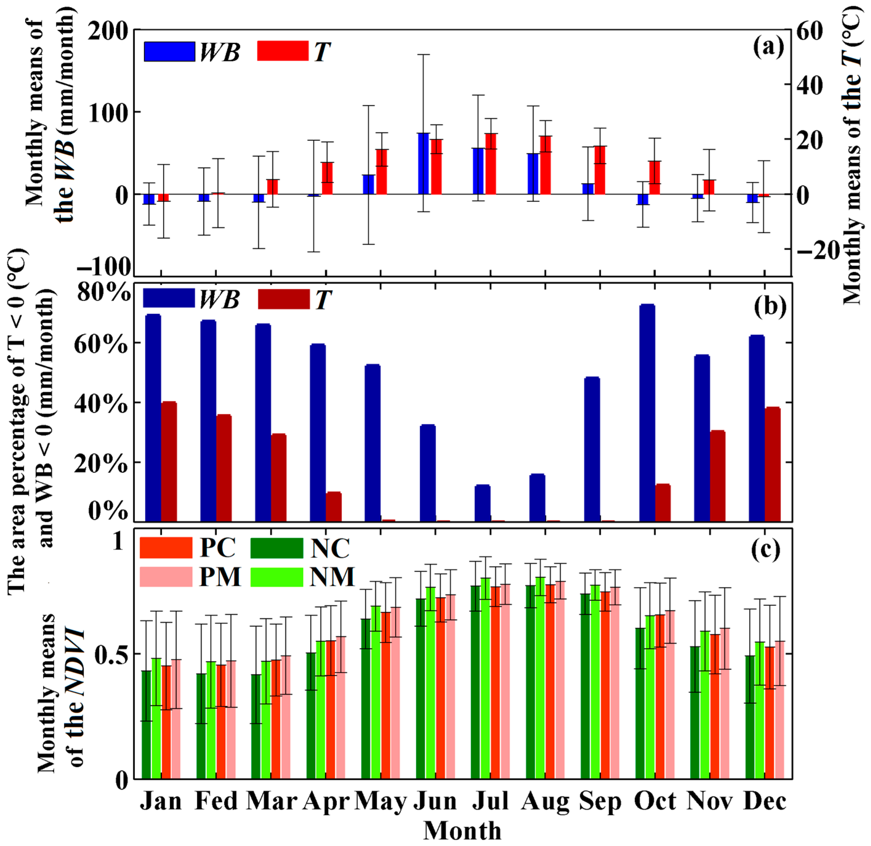
Forests are widely distributed in China (Figure 1). The climatic conditions of China are complex, and forest ecosystems are affected by drought [23,24]. China is dominated by an Asian monsoon climate, with T and WB (detailed information about these datasets can be found in Section 2.2.4) both showing obvious seasonal variations (Figure 2a,b). Occurrences of T ≥ 0 °C and WB ≥ 0 mm/month are concentrated during May–September, indicating that the warm and wet seasons are concentrated in May–September. With these climatic conditions, forest vigor also displays obvious seasonal variation, being highest during the growing season of May–September (Figure 2c). To reduce the interference of leaf fall, which typically occurs from October–December, only changes in forest vigor during the pregrowing (January–April) and growing (May–September) seasons are considered in this research.
2.2. Materials
2.2.1. Satellite-Derived Vegetation Index
The NDVI derived from the Moderate Resolution Imaging Spectroradiometer (MODIS) of Terra was used to monitor forest vigor in our research. The MOD13A3 (Version 6) dataset is a global monthly composite product that spans 2001–2015 with a spatial resolution of 1 km (https://search.earthdata.nasa.gov/, accessed 9 December 2020). The NDVI data were resampled to a spatial resolution of 0.01° by using ArcGIS (Version 10.2) (Esri, Environmental Systems Research Institute, New York, NY, USA). Additionally, to reflect the relative changes in forest vigor and to facilitate comparisons of forests, as well as to reduce the complex impacts of both biotic and abiotic factors on the NDVI itself, the raw NDVI data for each pixel were transformed into the deficit of NDVI (dNDVI) based on the maximum value of NDVI during 2001–2015 (Equation (1)). Compared to the original value of NDVI, the dNDVI reflected the change in grid NDVI that would be more directly related to the changes in water availability.
where x and y represent the longitude and latitude of every forest pixel, respectively; i ranges from January to September; and max represents the maximum value of the monthly NDVI during 2001–2015.
2.2.2. Forest Inventory Map
A forest distribution map derived from the Eighth Forest Inventory (2009–2013) of China was used in our research (Figure 1), which includes planted coniferous (PC), planted mixed (PM), natural coniferous (NC), and natural mixed (NM) forests [25]. The forest inventory map was obtained by remote sensing and a massive forest field survey, and can well-distinguish forests and nonforests [11]. To relate the distribution to the remote sensing NDVI, the map was first digitized and then converted into a raster file with the same spatial resolution of 0.01° through spatial adjustment and resampling using ArcGIS. Given that many researchers have discarded regions with NDVI values below a threshold to minimize soil background influences and enhance green forest signals [26,27,28], and the NDVI value of forests during the pregrowing season (January–April) is commonly greater than 0 [29], the regions with the minimum NDVI below 0 during January-December for the entire study period were excluded from analysis in this study. As a result, the area analyzed in this study occupied 90.93% of the total forest cover (Figure 1).
2.2.3. Meteorological Drought Index
Meteorological drought indexes, such as the Palmer Drought Severity Index (PDSI) [30], Standardized Precipitation Index (SPI) [31], and SPEI [14], are commonly used indicators for drought monitoring and assessment because they simplify complex interrelationships between many climate and climate-related parameters. The SPEI is a widely used and multiscalar drought index that can be effective for characterizing the cumulative effect of water availability on a pixel scale provided that a suitable time-scale is selected [11,12,21]. The SPEI is a standardized drought index that reflects the relative change of the water condition. The main steps employed to calculate SPEI were as follows: (1) The water balance represented as the difference (D) between precipitation (P) and potential evapotranspiration (PET obtained by Thornthwaite or Penman—Monteith methods) was calculated; (2) the D values were aggregated at various time-scales Equations (2) and (3) the series of D was fitted by a three-parameter log-logistic probability density function and converted by the standard normal distribution [14,18].
where i represents the calendar month, and j (months) is the timescale of the water balance aggregation.
Given that the Climatic Research Unit (CRU, University of East Anglia, UK) SPEI was calculated based on global monthly observed meteorological datasets that were interpolated to 0.5° and the PET was estimated using the well-known formula of FAO-56 Penman—Monteith [32,33], the CRU SPEI could characterize the actual water conditions more precisely on a regional scale [34,35]. In addition, the selected values of time-scales employed for capturing the cumulative effect were diverse in different research studies, with the longest time-scales of SPEI reaching 48 months [20]. Therefore, in this study, the monthly SPEI values with a 1–48 month time-scale derived from the latest CRU dataset (Version 2.5) were used (http://digital.csic.es/handle/10261/153475, accessed 10 March 2020). To match with other data, such as remote sensing NDVI and the forest map, only the SPEI datasets spanning 2001–2015 were selected and resampled to a spatial resolution of 0.01° using the nearest neighbor method of ArcGIS.
2.2.4. Environmental Temperature and Water Balance
To characterize environmental climatic conditions, the monthly observed meteorology datasets of CRU TS3.24.01 with a 0.5 degree spatial resolution (http://data.ceda.ac.uk/badc/cru/data/cru_ts/cru_ts_3.24.01/data/, accessed 9 December 2020) were obtained from the CEDA catalogue (the Natural Environment Research Council’s Data Repository for Atmospheric Science and Earth Observation) and used in this study, representing the basic data of CRU SPEI (Version 2.5). The datasets included the monthly temperature (K), monthly precipitation (mm/month), and daily potential evapotranspiration (mm/day). The environmental temperature and water balance were calculated according to the following steps. First, the total potential evapotranspiration was calculated for every month based on the daily potential evapotranspiration and the number of days. Second, the monthly WB was calculated using the monthly potential evapotranspiration and monthly precipitation (Equation (3)). Finally, the monthly averaged T and WB during 2001–2015 were calculated and resampled to a spatial resolution of 0.01°.
where WB is the monthly water balance; x and y represent the longitude and latitude of every forest pixel, respectively; i represents months ranging within January–September; and P and PET represent the monthly precipitation and monthly potential evapotranspiration, respectively.
2.3. Methods
2.3.1. Definition of Positive and Negative Roles of Water Availability in Forest Vigor
Our research defined the positive and negative roles of water availability in forest vigor based on the strongest correlation between dNDVI and SPEI. First, we determined Pearson’s correlation (r) between monthly dNDVI and SPEI for time-scales of 1–48 months during the period of 2001–2015 (Equation (4)). Secondly, for each pixel, the absolute maximum correlation coefficient (|r|max) was obtained by ENVI/IDL (Version 5.0) (Exelis Visual Information Solutions, Boulder, CO, USA) (Equation (5)). r was used to further characterize the strongest positive (rp) or negative (rn) correlations of forest vigor with water availability. Finally, the spatial distribution of rp and rn were determined by ArcGIS to show spatial patterns. In addition, their histograms for various forest types (PC, PM, NC, and NM) and different periods (pregrowing and growing seasons) were determined using MATLAB (R2012b) (MathWorks, Natick, MA, USA), respectively.
where x and y represent the longitude and latitude, respectively; i ranges within January-September; and j ranges within 1–48 months. Because r was calculated using values of dNDVI and SPEI for 15 years (N = 15, where “N” represents the number of data samples), and we selected the value of 0.05 as the significance level of the correlation coefficient, corresponding to the threshold of 0.514, the value of |r| > 0.514 (i.e., critical value) means significant at a 0.05 level [36].
2.3.2. Quantifying the Impacts of Environmental Climate, Seasonality, and Forest Types
Based on the environmental climate data (i.e., T and WB) and the strongest correlations (i.e., rp and rn) of forests with water availability, our research aimed to quantify the impacts of environmental climate on the dual roles (positive or negative correlations) of water availability in forest vigor among seasons (i.e., pregrowing season in January–April and growing season in May–September) and among forest types (i.e., planted and natural forests). First, we counted the ratio of the area (the number of pixels) of significantly positive (i.e., rp) and negative correlations (i.e., rn) to the whole calculation area (the number of pixels) for every 5 °C and every 20 mm/month for pregrowing and growing seasons, respectively, which we also named the area percentage. Second, the statistical relationships between the average value of T and WB and the area percentage of significant rp and rn in the same climatic condition were constructed using a linear regression model (i.e., y = ax + b) and an exponential regression model (i.e., y = a[exp(bx)] + c[exp(dx)]), respectively. Additionally, to further eliminate the influence of the heteroscedasticity of residuals, we also combined the fitting line of the weighted regression model with that of the linear regression model. To determine whether planted and natural forests exhibited response differences, the independent-samples t-test with a bootstrapped sampling method (1000 samples) was used to compare the differences in the area percentage of both significant rp and rn between planted and natural forests. Finally, to confirm whether any climatic threshold existed, which can indicate changes of the difference in the area percentage between significant rp and rn, two methods were used in the research: (1) The intersection points of two linear fitting lines were obtained as the environmental temperature thresholds, and (2) a series of the difference between the area percentage of significant rp and rn was calculated for various ordered groups of environmental water balance that ranged from large to small (e.g., WB > 220 mm/month, WB > 200 mm/month, WB > 180 mm/month, etc.) by using the paired t-test method. We found that the difference between significant rp and rn appears to be significant at a 0.05 statistical level when WB is greater than one, and the value is the threshold of WB. Additionally, the actual data of T or WB around each threshold were added in the research, respectively.
2.3.3. Sensitivity Analysis for the Time-Scales of SPEI
Recently, a number of studies have found that the cumulative effect of water availability on forest vigor is important, but selecting a suitable time-scale of the cumulative time is often arbitrary, which can range within 1–48 months [6,18,20]. Therefore, to determine whether the dual roles (i.e., positive and negative correlations) of water availability in forest vigor are sensitive to SPEI time-scales, we compared the difference in climatic thresholds among time-spans of 1–12, 1–24, 1–36, and 1–48 months. A detailed flow diagram of the analysis is shown in Figure 3.
3. Results
3.1. Dual Roles of Water Availability in Forest Vigor
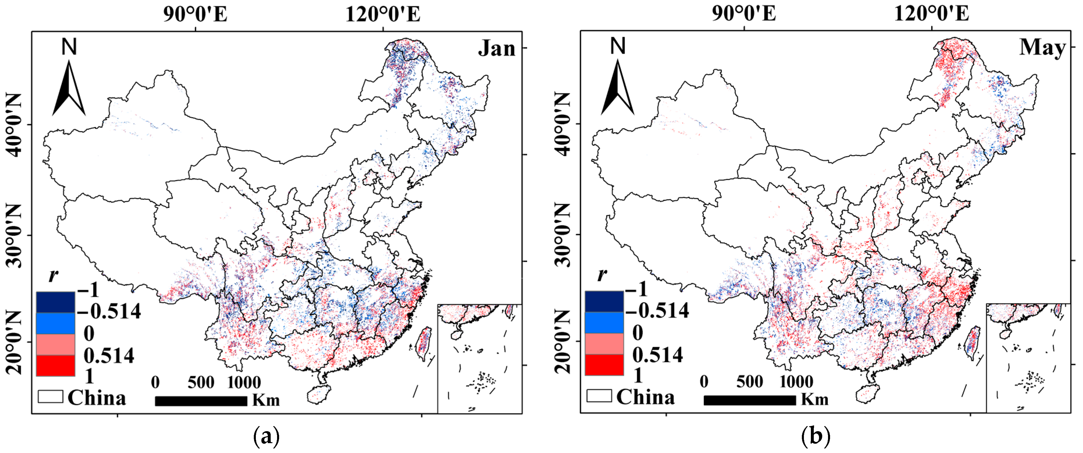
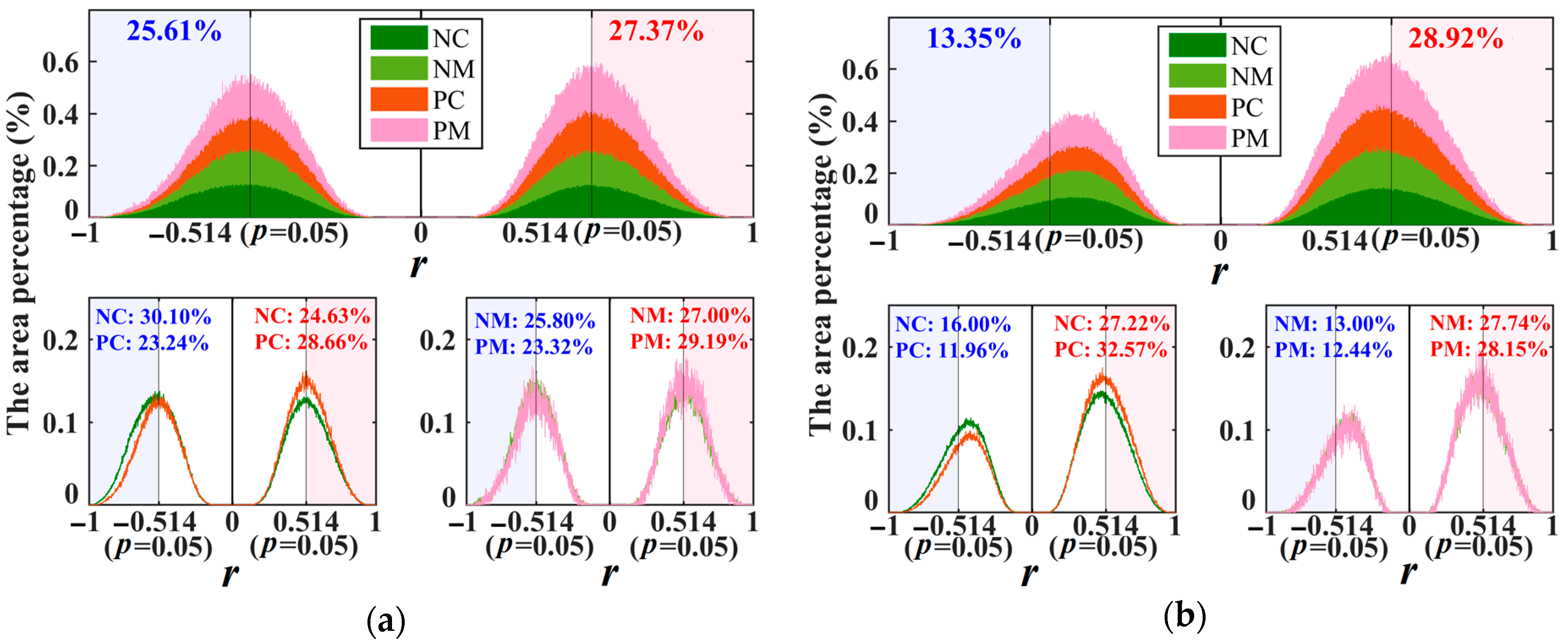
Based on the strongest correlations of forests with water availability, as characterized by the r corresponding to |r|max, our research showed that water availability played dual roles (i.e., positive or negative correlations) in forest vigor in China (Figure 4 and Figure S1). The positive (rp) and negative (rn) correlations both displayed great spatial and temporal heterogeneity (Figure 4 and Figure S1). The role of water availability was related to the season (i.e., pregrowing season and growing season), but was not related to the forest type (i.e., planted and natural). During the pregrowing season, the values of rp and rn exhibited a double peak curve. The double peak was concentrated at 0.514 and −0.514, respectively. This phenomenon can be found in all forests (i.e., PC, PM, NC, and NM) and suggested that nearly 50% of forests showed no significant change when the water availability increased or decreased (Figure 5a).
Additionally, for all forests, there was no difference in the area percentage of significant rp (27.37%) and significant rn (25.61%) in the pregrowing season; during the growing season, however, the significantly negative role of water decreased (13.35%) and the significantly positive role of water increased (28.92%) (Figure 5b). This demonstrates that the forest region with a significant positive correlation was mostly observed during the growing season. Furthermore, the phenomenon can also be found in all forest types, as the insets of Figure 5 show. To eliminate interference of the normal variations for forest vigor, the regions with the significant positive and negative correlations (i.e., |r| > 0.514) were selected and analyzed further.
3.2. Factors Impacting the Roles of Water Availability
3.2.1. Temperature Dependency
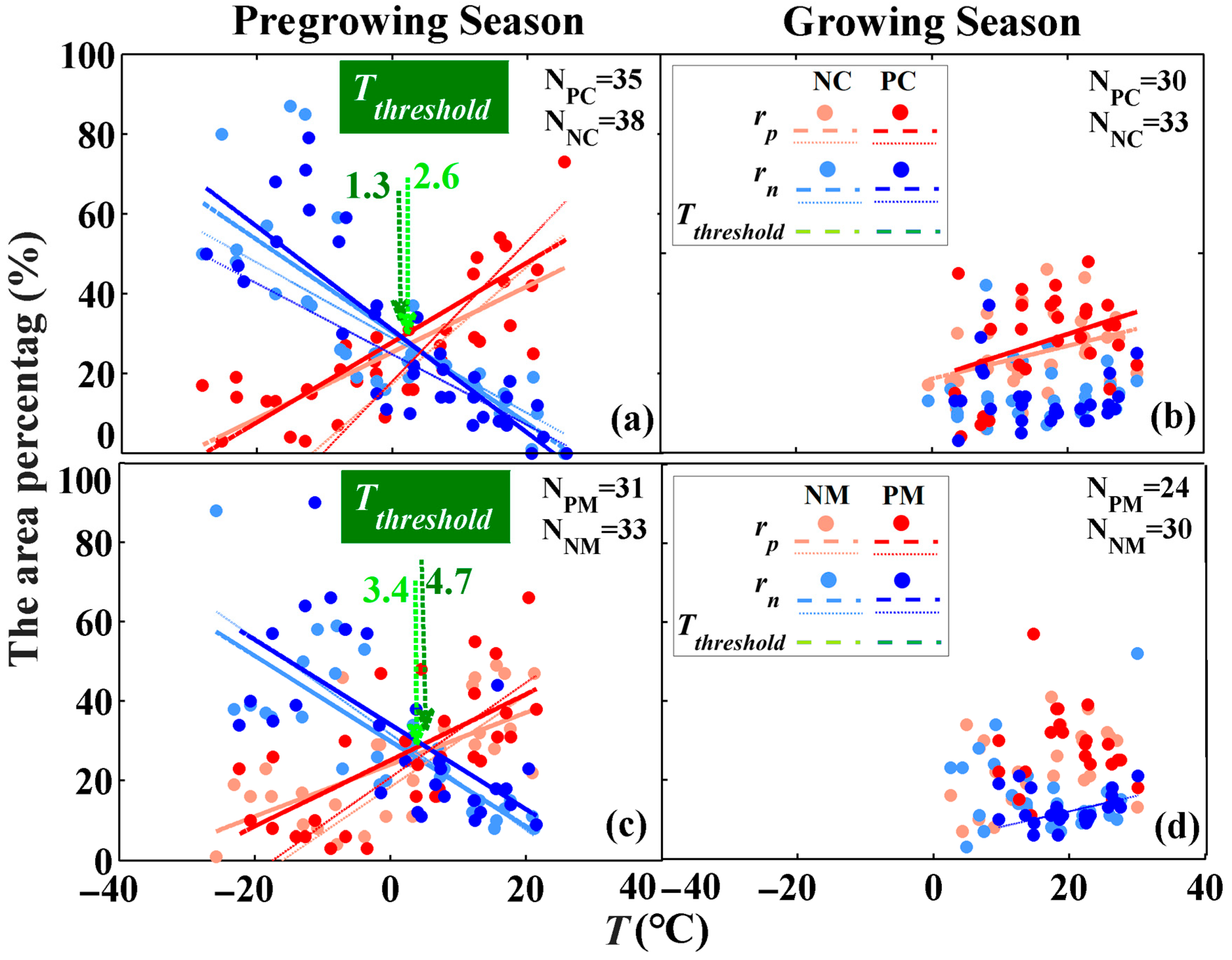
The roles of water availability in forest vigor were highly dependent on the temperature and the time (i.e., season of concern), but independent of the forest type (i.e., planted and natural forests). During the pregrowing season, the area percentages of significant positive/negative correlations for all forests were linear increases/decreases with increased T (Figure 6a,c). The differences in the area percentage between positive and negative correlations also changed with increases in T (Figure 6a,c); that is, the role of water availability in forest vigor was related to T. Specifically, the forest regions with a negative correlation were mostly located in cooler environments (T ≤ Tthreshold), while those with a positive correlation were mainly situated in warmer environments (T > Tthreshold) (Figure 7). The value of Tthreshold varied according to the forest type, with 1.3 (−0.85~2.60), 2.6 (2.42~2.87), 4.7 (4.55~6.65), and 3.4 (3.30~6.90) °C for PC, NC, PM, and NM, respectively (Figure 6a,c and Figure 7). These results indicated that T during the pregrowing season should be considered to better explore the impacts of drought. During the growing season, however, both the positive and negative correlations of all forests exhibited no obvious difference (Figure 6b,d); that is, the T does not show any effect on the differences in positive and negative roles of water availability during the growing season.
Despite the values of Tthreshold being somewhat different for planted and natural forests, their relationship of temperature dependency is similar. Moreover, there were no significant differences in the area percentage of positive/negative correlations between planted and natural forests (i.e., PC vs. NC and PM vs. NM) during the pregrowing season and growing season, because all of the p-values of the independent-samples t-test with a bootstrapped sampling method (1000 samples) were greater than 0.05 (Table S1). This indicates that the role of water in vegetation vigor was independent of the forest type.
3.2.2. Water Balance Dependency
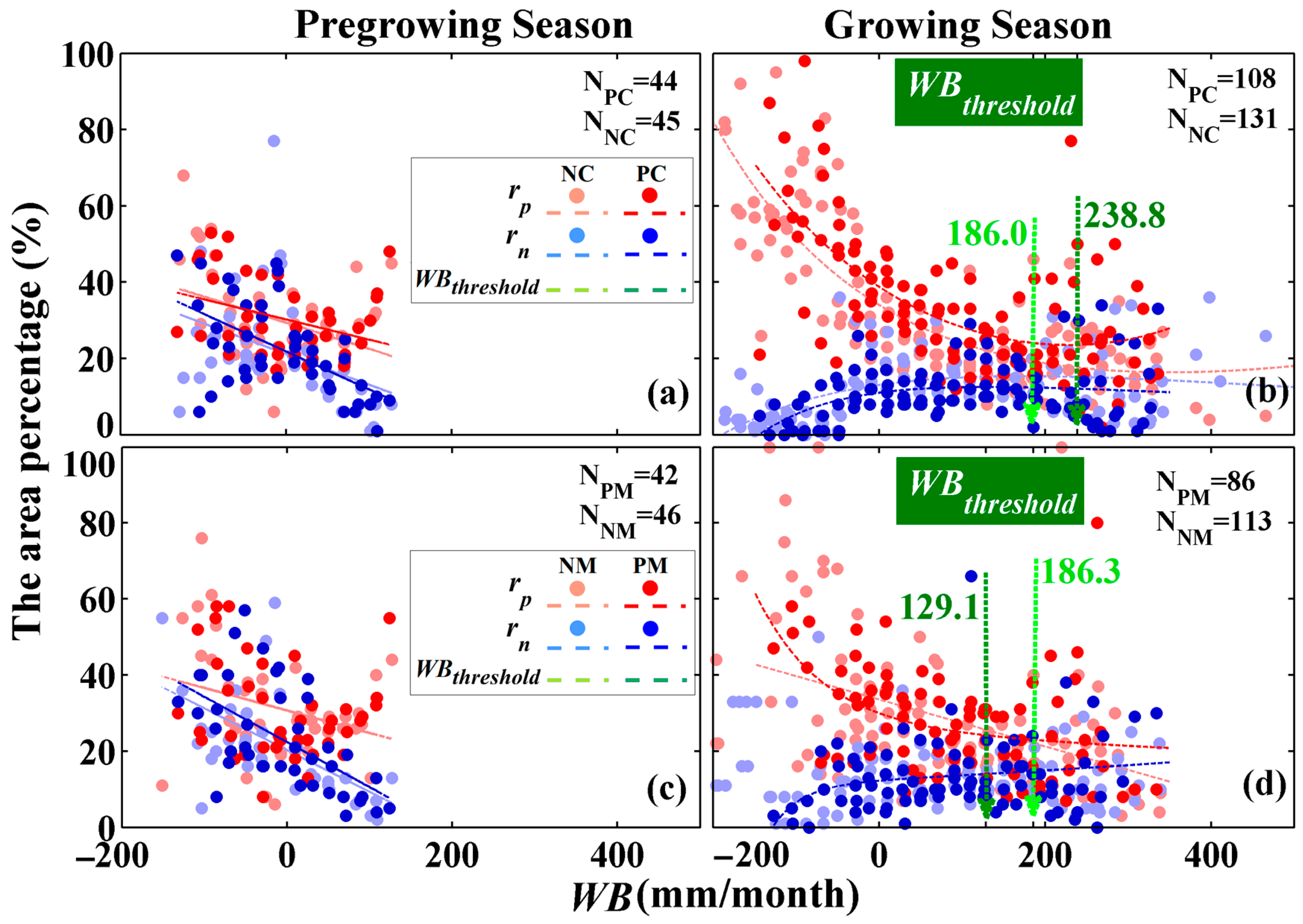
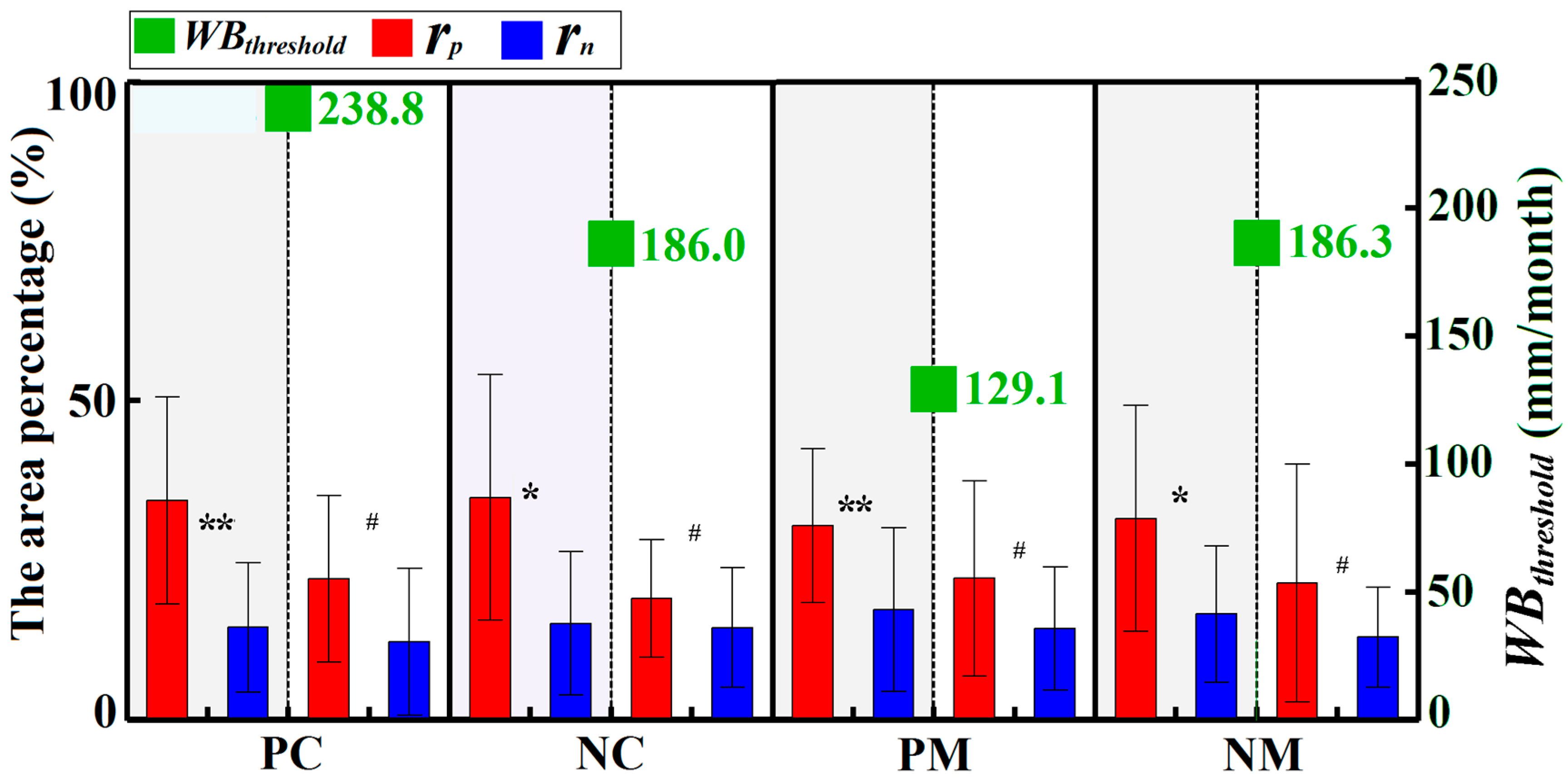
The roles of water availability in forest vigor were also highly dependent on environmental WB, and differed among the pregrowing season and growing season. Similar to the temperature dependency, the water balance dependency is not related to the forest type, as planted and natural forests show a similar relationship. During the pregrowing season, the area percentages of significant positive and negative correlations for all forests both linearly decreased with increases in WB (Figure 8a,c). There was no difference in the area percentages between significant positive and negative correlations, indicating that the environmental WB did not explain the differences between positive and negative roles of water availability in forest vigor during the pregrowing season. During the growing season, however, the area percentages of significant positive/negative correlations for most of the forests exponentially decreased/increased with increases in environmental WB (Figure 8b,d). At the same time, the differences in the area percentages between significant positive and negative correlations decreased gradually (Figure 8b,d). In drier environments (i.e., WB ≤ WBthreshold), most forests had a positive relationship with water availability (Figure 9). In contrast, in wetter environments (i.e., WB > WBthreshold), there was no difference in area percentages between significant positive and negative correlations (Figure 9). These results indicated that the role of water in vegetation vigor was related to environmental WB, which played a positive role in relatively drier environments. The values of WBthreshold were also related to the forest type, with values of 238.8 (241.4~238.8), 186.0 (189.5~186.0), 129.1 (129.7~129.1), and 186.3 (186.5~186.3) mm/month for PC, NC, PM, and NM, respectively (Figure 8b,d and Figure 9). These results indicated that WB during the growing season should be taken into consideration to better explore the effects of drought.
Despite the values of WBthreshold being somewhat different for planted and natural forests, their general relationship of water balance dependency is similar. The independent-samples t-test with a bootstrapped sampling method (1000 samples) indicated that nonsignificant differences exist in the area percentage of significant positive/negative correlations between planted and natural forests (i.e., PC vs. NC and PM vs. NM) during the pregrowing season and growing season at a 0.05 level (Table S2).
3.3. Sensitivity of the Roles of Water Availability in Forest Vigor to the SPEI Time-Scale
Comparisons of three time-spans of SPEI (i.e., SPEI 1–12, SPEI 1–24, SPEI 1–36, and SPEI 1–48) showed that the T dependency and WB dependency of the water availability impact on forest vigor were independent of the SPEI time-scale, with similar Tthreshold and WBthreshold values for a certain forest type (Figure 10). Specifically, all results demonstrated that environmental climate and time (pregrowing season or growing season) jointly affected the dual roles of water availability in forest vigor and there were similar climatic thresholds for the different SPEI time-spans.
4. Discussion
4.1. Uncertainties and Prospects
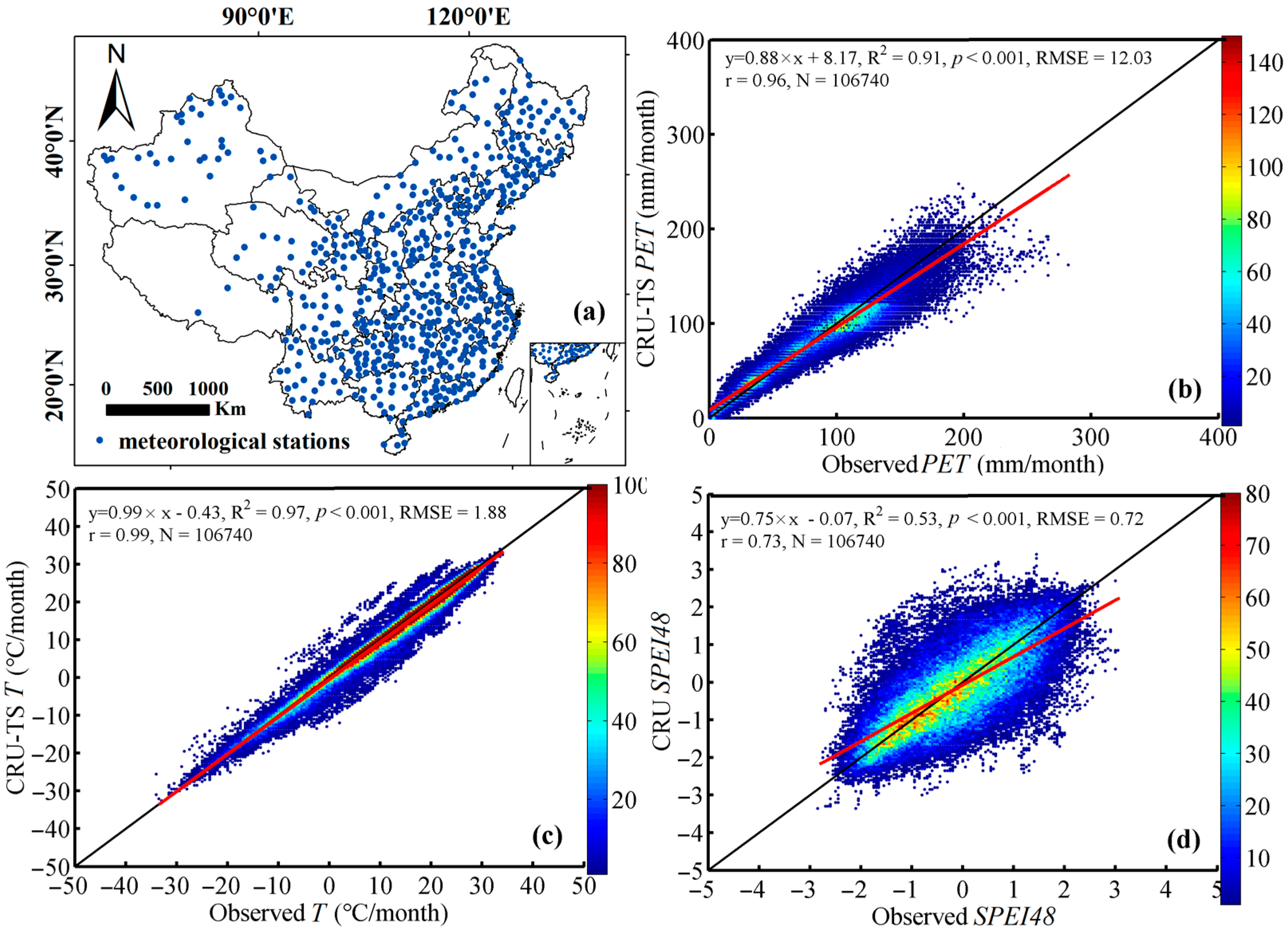
The CRU-TS grid dataset (e.g., P, PET, and T) and their integrated index (i.e., CRU SPEI) were used in our research. To assess the suitability of these CRU data, we also compared them with site-based values (Figure 11). Specifically, we calculated PET and SPEI based on 593 stations of observed meteorological variables in China and compared them with those in CRU datasets. We found that all of the CRU data were consistent with those derived from observation stations, demonstrating a high consistency (Figure 11a–d and Figure S2a–d). Therefore, the CRU data were suitable for this study.
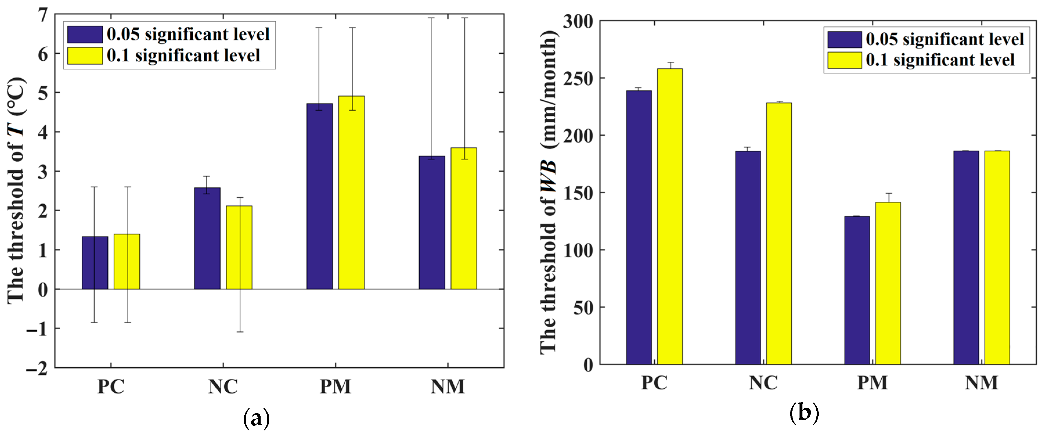
Because the statistical significance level of 0.05 (i.e., p = 0.05) is commonly used in related research, our research focused on the area with |r| < 0.514 (i.e., p < 0.05). However, the correlation is an estimate with associated uncertainty and statistical significance itself is a rather artificial criterion. Therefore, we compared the results of the statistical significance level of 0.05 with that of 0.1 (i.e., |r| < 0.441). We found that there was no difference in the thresholds between two significant levels (Figure 12), because the p values of the t-test (with a bootstrapped sampling method, 1000 samples) for temperature and water balance thresholds were 0.899 and 0.191, respectively.
Despite these efforts, some uncertainties still remain, such as the occurrence of possible errors during the matching process between the forest distribution map and remote sensing images, as well as in the spatial resolution resampling process. Therefore, more matchable data on time and space are needed in the future to continue to decrease the uncertainties. In addition, changes in forest vigor may be affected by other factors (e.g., insects, diseases, and fire) [23,37], as well as interactions among them and climate change/drought [38,39,40], which adds uncertainties to our results. However, the effect of these factors on forests are always represented by relatively low percentages [37], for example, <0.17% of the forest area in Yunnan was damaged by fire during 2001–2014 [12], and such uncertainties would not change our main conclusions. In addition, the background of global warming and the changes in drought frequency, duration, and intensity [16,41] will require some consideration in future study [23].
The synergic use of multiple remote sensing data (e.g., optical and microwave remote sensing, as well as light detection and ranging (LiDAR) data), could provide better results, because current data still present some uncertainties. For instance, optical remote sensing data (e.g., the vegetation index based on reflectivity) have been widely used to investigate the responses of forests to climate change due to them providing continuous information on forest dynamics, both temporally and spatially [42,43]. However, optical remote sensing only acquires canopy surface information [44]. In contrast, microwave remote sensing (e.g., synthetic aperture radar (SAR)) is superior to optical remote sensing in reducing high-resolution imagery of the Earth’s surface in all weather conditions [45,46], and LiDAR techniques have been proven to accurately capture the three-dimensional structure of a vegetation ecosystem [47,48]. However, SAR and LiDAR data also have limitations, such as limitations in temporal and spatial coverage, uncertainties in estimation, expensive datasets, and difficulties in data processing [49,50,51]. Therefore, a growing number of research focused on the synergic use of multisensor optical, SAR, and LiDAR, could provide better results as all data types complement each other, overcoming their respective limitations [49].
4.2. Adjustment Mechanisms of Environmental Climate and Seasonality
Our study found that the dual roles of water availability in forest vigor were jointly controlled by the environmental T and the seasonality (i.e., pregrowing season or growing season). In this study, we found that the roles of water availability in forest vigor in China had both positive and negative roles (Figure 4 and Figure 5 and Figure S1), which is consistent with other research [6,20]. Specifically, the negative role of water availability in forest vigor was mainly found in regions of T ≤ Tthreshold during the pregrowing season. The Tthreshold values ranged within 1.3–4.7 °C and varied according to the forest type, consistent with other phenological research which found that a temperature lower than 5 °C is too cold for forest growth during the pregrowing season [52,53,54]. As a result, forests located in cold regions (T ≤ Tthreshold) are not limited by water availability, but by temperature [22]. As a result, there was no difference in the frequency of rp and rn in the pregrowing season, which means that nearly 50% of forests showed no significant change when the water availability increased or decreased at a 0.05 significant level (i.e., |r| > 0.514) (Figure 5). Additionally, given that temperature is usually negatively correlated with water availability [55], the negative correlation is probably an indirectly response of those forests located in cold regions (T ≤ Tthreshold) to water availability during the pregrowing season (Figure 13a). With increases in environmental T, the importance of water availability for forest vigor increased, which caused the area percentage of the positive correlations to increase accordingly (Figure 13a,b). As T further increased and reached a threshold (i.e., T > Tthreshold), the main limiting factor for forests became water availability and thus the positive role of water availability appeared (Figure 6, Figure 7 and Figure 13a,b).
Additionally, the dual roles of water availability in forest vigor were driven by the environmental WB and the seasonality. Previous research indicated that forest vigor during the growing season is commonly controlled by water availability [19,22], especially for drier regions of WB ≤ WBthreshold (Figure 13b). Therefore, they mainly show a positive response to water availability (Figure 8 and Figure 9). With increases in environmental WB, the importance of water availability for forests decreases, while the impacts caused by other limited factors (e.g., nutrients, diseases, and insects) emerge [23,37,56] (Figure 13b,c). As a result, forests located in wet regions (i.e., WB > WBthreshold) showed not only positive correlations, but also negative correlations, with water availability, which caused nonsignificant differences in the area percentages between the positive and negative correlations (Figure 8b,d). The results are consistent with other relevant research showing a negative correlation in wet regions [6,20] (Figure 13c). The WBthreshold is a key parameter for determining whether or not the forest is limited by water availability. In this study, we found WBthreshold of 129.1–238.8 mm/month, which varied according to the forest type (Figure 8 and Figure 9). In addition, values of WBthreshold were not sensitive to the selected SPEI time-scale (Figure 10), implying that these thresholds were invariant and useful for evaluating the effects of drought.
However, the roles of water availability in forest vigor were vegetation type-independent. The planted and natural forests showed similar rules due to the fact that temperature and water were the necessary resources for all forests [22,54]; that is, both environmental climate (i.e., T and WB) and seasonality (i.e., pregrowing season or growing season) adjusted the sensitivity of forests to temperature and water. Therefore, planted and natural forests exhibited consistent phenomena of temperature and water balance dependency (Figure 6 and Figure 8). However, the forest age, canopy height, stock volume, and other factors may lead to the differences in the sensitivity of forests to temperature and water availability [11,15,57], which means that the values of Tthreshold and WBthreshold varied to a certain degree with forest type (Figure 7 and Figure 9).
5. Conclusions
Water is an important climatic resource for vegetation. However, due to the complex spatio-temporal relationship among climatic factors and vegetation, water shows both positive and negative correlations with forest vigor, and the reasons for the negative impact are not well-known. In this study, we conducted a multiperspective analysis for the forests in China. Specifically, to reveal the underlying mechanism causing the positive and negative role of water availability, we considered the influences of multiple factors (i.e., temperature and water balance, forest types, season differences, and multiple time scales of water availability) by combining multiple data (e.g., satellite-derived NDVI and the multiple time-scale SPEIs). The results indicated that the negative role of water availability in forest vigor mainly occurred in regions of T ≤ Tthreshold during the pregrowing season. In comparison, positive roles mainly occurred in warmer regions (T > Tthreshold) during the pregrowing season and in wetter regions (WB > WBthreshold) during the growing season. The Tthreshold and WBthreshold were vegetation type-dependent, with values ranging from 1.3 to 4.7 °C for Tthreshold and 129.1 to 238.8 mm/month for WBthreshold. These results revealed that both environmental climate and seasonality should be considered when monitoring or predicting the impacts of drought on the satellite-derived forest vigor (i.e., NDVI). Therefore, to explore the direct effects of drought on forests in the future, relevant research should focus on forests limited by water availability.
Supplementary Materials
The following are available online at https://www.mdpi.com/2072-4292/13/1/91/s1, Table S1: The results of independent-samples t-test for temperature dependency, Table S2: The results of independent-samples t-test for water balance dependency, Table S3: The environmental climatic thresholds and their ranges for various time scales, Table S4: The environmental climatic thresholds and their ranges for a 0.1 statistically significant level, Figure S1: Spatial distribution of the strongest correlations (the r corresponds to |r|max) of forest vigor with water availability in China, Figure S2: Comparisons between CRU data and the counterparts derived from meteorological stations.
Author Contributions
Conceptualization, H.L. and T.Z.; Data curation, H.L., T.Z., P.X., P.Y. and J.L.; Formal analysis, H.L., T.Z. and X.L.; Funding acquisition, T.Z. and P.S.; Investigation, H.L. and T.Z.; Methodology, H.L. and X.L.; Project administration, T.Z. and P.S.; Resources, H.L., T.Z., P.S., R.M. and X.Z.; Software, H.L., X.L. and P.X.; Supervision, T.Z. and P.S.; Validation, T.Z., X.L., P.S., R.M. and X.Z.; Visualization, H.L.; Writing—Original draft, H.L. and T.Z.; Writing—Review & editing, T.Z., X.L., P.S., R.M., X.Z., P.X., P.Y. and J.L. All of the authors contributed to the manuscript and approved the final version. All authors have read and agreed to the published version of the manuscript.
Funding
We would like to thank the high-performance computing support from the Center for Geodata and Analysis, Faculty of Geographical Science, Beijing Normal University [https://gda.bnu.edu.cn/]. This study was supported by the Major Project of Qinghai province (2019-SF-A12), the second Tibetan Plateau Scientific Expedition and Research Program (2019QZKK0405), and the National Natural Science Foundation of China (41621061 and 41571185).
Institutional Review Board Statement
Not applicable.
Informed Consent Statement
Not applicable.
Data Availability Statement
Data is contained within the article or supplementary material.
Conflicts of Interest
The authors declare no conflict of interest.
References
- Dixon, R.K. Carbon Pools and flux of Global Forest Ecosystems. Science 1994, 263, 185–190. [Google Scholar] [CrossRef]
- Pan, Y.; Birdsey, R.A.; Phillips, O.L.; Jackson, R.B. The structure, distribution, and biomass of the world’s forests. Annu. Rev. Ecol. Evol. Syst. 2013, 44, 593–622. [Google Scholar] [CrossRef] [Green Version]
- McKinley, D.C.; Ryan, M.G.; Birdsey, R.A.; Giardina, C.P.; Harmon, M.E.; Heath, L.S.; Houghton, R.A.; Jackson, R.B.; Morrison, J.F.; Murray, B.C.; et al. A synthesis of current knowledge on forests and carbon storage in the united states. Ecol. Appl. 2011, 21, 1902–1924. [Google Scholar] [CrossRef] [Green Version]
- Dai, A. Increasing drought under global warming in observations and models. Nat. Clim. Chang. 2013, 3, 52–58. [Google Scholar] [CrossRef]
- O’Brien, M.J.; Engelbrecht, B.M.J.; Joswig, J.; Pereyra, G.; Schuldt, B.; Jansen, S.; Kattge, J.; Landhäusser, S.M.; Levick, S.R.; Preisler, Y. A synthesis of tree functional traits related to drought-induced mortality in forests across climatic zones. J. Appl. Ecol. 2017, 54. [Google Scholar] [CrossRef]
- Zhang, Q.; Kong, D.; Singh, V.P.; Shi, P. Response of vegetation to different time-scales drought across China: Spatiotemporal patterns, causes and implications. Glob. Planet. Chang. 2017, 152, 1–11. [Google Scholar] [CrossRef] [Green Version]
- Khalifa, M.; Elagib, N.A.; Ribbe, L.; Schneider, K. Spatio-temporal variations in climate, primary productivity and efficiency of water and carbon use of the land cover types in Sudan and Ethiopia. Sci. Total Environ. 2018, 624, 790–806. [Google Scholar] [CrossRef]
- Zhao, A.; Zhang, A.; Cao, S.; Liu, X.; Liu, J.; Cheng, D. Responses of vegetation productivity to multi-scale drought in Loess Plateau, China. Catena 2018, 163, 165–171. [Google Scholar] [CrossRef]
- Hua, T.; Wang, X.; Zhang, C.; Lang, L.; Li, H. Responses of vegetation activity to drought in northern China. Land Degrad. Dev. 2017, 28, 1913–1921. [Google Scholar] [CrossRef]
- Gao, S.; Liu, R.; Zhou, T.; Fang, W.; Yi, C.; Lu, R.; Zhao, X.; Luo, H. Dynamic responses of tree-ring growth to multiple dimensions of drought. Glob. Chang. Biol. 2018, 24, 5380–5390. [Google Scholar] [CrossRef] [Green Version]
- Luo, H.; Zhou, T.; Wu, H.; Zhao, X.; Wang, Q.; Gao, S.; Li, Z. Contrasting Responses of Planted and Natural Forests to Drought Intensity in Yunnan, China. Remote Sens. 2016, 8, 635. [Google Scholar] [CrossRef] [Green Version]
- Luo, H.; Zhou, T.; Yi, C.; Xu, P.; Zhao, X.; Gao, S.; Liu, X. Stock Volume Dependency of Forest Drought Responses in Yunnan, China. Forests 2018, 9, 209. [Google Scholar] [CrossRef] [Green Version]
- Wu, D.; Zhao, X.; Liang, S.; Zhou, T.; Huang, K.; Tang, B.; Zhao, W. Time-lag effects of global vegetation responses to climate change. Glob. Chang. Biol. 2015, 21, 3520–3531. [Google Scholar] [CrossRef] [PubMed]
- Vicente-Serrano, S.M.; Begueria, S.; Lopez-Moreno, J.I. A Multiscalar Drought Index Sensitive to Global Warming: The Standardized Precipitation Evapotranspiration Index. J. Clim. 2010, 23, 1696–1718. [Google Scholar] [CrossRef] [Green Version]
- Xu, P.; Zhou, T.; Zhao, X.; Luo, H.; Gao, S.; Li, Z.; Cao, L. Diverse responses of different structured forest to drought in Southwest China through remotely sensed data. Int. J. Appl. Earth Obs. Geoinf. 2018, 69, 217–225. [Google Scholar] [CrossRef]
- Li, Z.; Zhou, T.; Zhao, X.; Huang, K.; Gao, S.; Wu, H.; Luo, H. Assessments of Drought Impacts on Vegetation in China with the Optimal Time Scales of the Climatic Drought Index. Int. J. Environ. Res. Public Health 2015, 12, 7615–7634. [Google Scholar] [CrossRef] [Green Version]
- Carlson, T.N.; Ripley, D.A. On the relation between NDVI, fractional vegetation cover, and leaf area index. Remote Sens. Environ. 1997, 62, 241–252. [Google Scholar] [CrossRef]
- Vicente-Serrano, S.M.; Gouveia, C.; Julio Camarero, J.; Begueria, S.; Trigo, R.; Lopez-Moreno, J.I.; Azorin-Molina, C.; Pasho, E.; Lorenzo-Lacruz, J.; Revuelto, J.; et al. Response of vegetation to drought time-scales across global land biomes. Proc. Natl. Acad. Sci. USA 2013, 110, 52–57. [Google Scholar] [CrossRef] [Green Version]
- Lévesque, M.; Saurer, M.; Siegwolf, R.; Eilmann, B.; Rigling, A. Drought response of five conifer species under contrasting water availability suggests high vulnerability of Norway spruce and European larch. Glob. Chang. Biol. 2013, 19, 3184–3199. [Google Scholar] [CrossRef]
- Xu, H.J.; Wang, X.P.; Zhao, C.Y.; Yang, X.M. Diverse responses of vegetation growth to meteorological drought across climate zones and land biomes in northern China from 1981 to 2014. Agric. For. Meteorol. 2018, 262, 1–13. [Google Scholar] [CrossRef]
- Huang, K.; Yi, C.; Wu, D.; Zhou, T.; Zhao, X.; Blanford, W.J.; Wei, S.; Wu, H.; Ling, D.; Li, Z. Tipping point of a conifer forest ecosystem under severe drought. Environ. Res. Lett. 2015, 10, 024011. [Google Scholar] [CrossRef]
- Xu, H.J.; Wang, X.P.; Yang, T.B. Trend shifts in satellite-derived vegetation growth in Central Eurasia, 1982–2013. Sci. Total Environ. 2016, 579, 1658. [Google Scholar] [CrossRef]
- Zhang, C.; Ju, W.; Chen, J.M.; Wang, X.; Yang, L.; Zheng, G. Disturbance-induced reduction of biomass carbon sinks of China’s forests in recent years. Environ. Res. Lett. 2015, 10, 114021. [Google Scholar] [CrossRef]
- Li, Z.; Xiao, J.; Yu, Z.; Yi, Z.; Jing, L.; Han, X. Drought events and their effects on vegetation productivity in China. Ecosphere 2016, 7, e01591. [Google Scholar]
- State Forestry Administration of the People’s Republic of China. The Main Results at Eighth National Forest Resources Inventory (2009–2013). 2015. Available online: http://www.forestry.gov.cn/main/65/content-659670.html (accessed on 8 October 2014).
- Tang, B.H.; Shao, K.; Li, Z.L.; Wu, H.; Tang, R. An improved NDVI-based threshold method for estimating land surface emissivity using MODIS satellite data. Int. J. Remote Sens. 2015, 36, 1–15. [Google Scholar] [CrossRef]
- Liu, Y.; Wu, L.; Yue, H. Biparabolic NDVI-Ts Space and Soil Moisture Remote Sensing in an Arid and Semi arid Area. Can. J. Remote Sens. 2015, 41, 159–169. [Google Scholar] [CrossRef]
- Wu, X.; Liu, H.; Li, X.; Ciais, P.; Babst, F.; Guo, W.; Zhang, C.; Magliulo, V.; Pavelka, M.; Liu, S.; et al. Differentiating drought legacy effects on vegetation growth over the temperate Northern Hemisphere. Glob. Chang. Biol. 2017. [Google Scholar] [CrossRef]
- Defries, R.S.; Townshend, J.R.G. NDVI-derived land cover classifications at a global scale. Int. J. Remote Sens. 1994, 15, 3567–3586. [Google Scholar] [CrossRef]
- Palmer, W. Meteorological Drought; US Department of Commerce Weather Bureau: Washington, DC, USA, 1965; pp. 5–58.
- McKee, T.B.; Doesken, N.J.; Kleist, J. The relationship of drought frequency and duration to time scales. In Proceedings of the 8th Conference on Applied Climatology, American Meteorological Society, Anaheim, CA, USA, 17–22 January 1993; pp. 179–184. [Google Scholar]
- Harris, I.; Jones, P.D.; Osborn, T.J.; Lister, D.H. Updated high-resolution grids of monthly climatic observations-The cru ts3.10 dataset. Int. J. Climatol. 2014, 34, 623–642. [Google Scholar] [CrossRef] [Green Version]
- Allen, R.; Pereira, L.; Raes, D.; Smith, M.; Allen, R.G.; Pereira, L.S.; Martin, S. Crop Evapotranspiration. Guidelines for Computing Crop Water Requirements; FAO Irrigation and Drainage: Rome, Italy, 1998; pp. 1–300. [Google Scholar]
- Vicente-Serrano, S.M.; Camarero, J.J.; Azorin-Molina, C. Diverse responses of forest growth to drought time-scales in the Northern Hemisphere. Glob. Ecol. Biogeogr. 2015, 23, 1019–1030. [Google Scholar] [CrossRef] [Green Version]
- Peng, J.; Wu, C.; Zhang, X.; Wang, X.; Gonsamo, A. Satellite detection of cumulative and lagged effects of drought on autumn leaf senescence over the Northern Hemisphere. Glob. Chang. Biol. 2019, 25, 2174–2188. [Google Scholar] [CrossRef] [PubMed]
- Ho, R. Handbook of Univariate and Multivariate Data Analysis with IBM SPSS, 2nd ed.; Chapman and Hall: London, UK, 2015; pp. 219–232. [Google Scholar]
- Chen, L.; Huang, J.G.; Dawson, A.; Zhai, L.; Stadt, K.J.; Comeau, P.G.; Whitehouse, C. Contributions of insects and droughts to growth decline of trembling aspen mixed boreal forest of western Canada. Glob. Chang. Biol. 2018, 24, 655–667. [Google Scholar] [CrossRef] [PubMed]
- Kolb, T.E.; Fettig, C.J.; Ayres, M.P.; Bentz, B.J.; Hicke, J.A.; Mathiasen, R.; Stewart, J.E.; Weed, A.S. Observed and anticipated impacts of drought on forest insects and diseases in the United States. For. Ecol. Manag. 2016, 380, 321–334. [Google Scholar] [CrossRef]
- Seidl, R.; Thom, D.; Kautz, M.; Martin-Benito, D.; Peltoniemi, M.; Vacchiano, G.; Wild, J.; Ascoli, D.; Petr, M.; Honkaniemi, J. Forest disturbances under climate change. Nat. Clim. Chang. 2017, 7, 395. [Google Scholar] [CrossRef] [PubMed] [Green Version]
- Hanson, P.J.; Weltzin, J.F. Drought disturbance from climate change: Response of United States forests. Sci. Total Environ. 2000, 262, 205–220. [Google Scholar] [CrossRef]
- Allen, C.D.; Macalady, A.K.; Chenchouni, H.; Bachelet, D.; McDowell, N.; Vennetier, M.; Kitzberger, T.; Rigling, A.; Breshears, D.D.; Hogg, E.H.; et al. A global overview of drought and heat-induced tree mortality reveals emerging climate change risks for forests. For. Ecol. Manag. 2010, 259, 660–684. [Google Scholar] [CrossRef] [Green Version]
- Dorman, M.; Svoray, T.; Perevolotsky, A.; Sarris, D. Forest performance during two consecutive drought periods: Diverging long-term trends and short-term responses along a climatic gradient. For. Ecol. Manag. 2013, 310, 1–9. [Google Scholar] [CrossRef]
- Xu, P.; Zhou, T.; Yi, C.; Luo, H.; Zhao, X.; Fang, W.; Gao, S.; Liu, X. Impacts of Water Stress on Forest Recovery and Its Interaction with Canopy Height. Int. J. Environ. Res. Public Health 2018, 15, 1257. [Google Scholar] [CrossRef] [Green Version]
- Lu, D. The potential and challenge of remote sensing-based biomass estimation. Int. J. Remote Sens. 2006, 27, 1297–1328. [Google Scholar] [CrossRef]
- Sinha, S.; Santra, A.; Sharma, L.; Jeganathan, C.; Nathawat, M.S.; Das, A.K.; Mohan, S. Multi-polarized Radarsat-2 satellite sensor in assessing forest vigor from above ground biomass. J. For. Res. 2018, 29, 1139–1145. [Google Scholar] [CrossRef]
- Sinha, S.; Jeganathan, C.; Sharma, L.K.; Nathawat, M.S.; Das, A.K.; Mohan, S. Developing synergy regression models with space-borne ALOS PALSAR and Landsat TM sensors for retrieving tropical forest biomass. J. Earth Syst. Ence 2016, 125, 725–735. [Google Scholar] [CrossRef] [Green Version]
- Hu, T.; Zhang, Y.Y.; Su, Y.; Zheng, Y.; Guo, Q. Mapping the Global Mangrove Forest Aboveground Biomass Using Multisource Remote Sensing Data. Remote Sens. 2020, 12, 1690. [Google Scholar] [CrossRef]
- Bergen, K.M.; Goetz, S.J.; Dubayah, R.O.; Henebry, G.M.; Hunsaker, C.T.; Imhoff, M.L.; Nelson, R.F.; Parker, G.G.; Radeloff, V.C. Remote sensing of vegetation 3-D structure for biodiversity and habitat: Review and implications for lidar and radar spaceborne missions. J. Geophys. Res. 2009, 114, G00E06. [Google Scholar] [CrossRef] [Green Version]
- Sinha, S.; Jeganathan, C.; Sharma, L.K.; Nathawat, M.S. A review of radar remote sensing for biomass estimation. Int. J. Environ. Ence Technol. 2015, 12, 1779–1792. [Google Scholar] [CrossRef] [Green Version]
- Tianyu, H.; Yanjun, S.; Baolin, X.; Jin, L.; Xiaoqian, Z.; Jingyun, F.; Qinghua, G. Mapping Global Forest Aboveground Biomass with Spaceborne LiDAR, Optical Imagery, and Forest Inventory Data. Remote Sens. 2016, 8, 565. [Google Scholar]
- Su, Y.; Guo, Q.; Xue, B.; Hu, T.; Alvarez, O.; Tao, S.; Fang, J. Spatial distribution of forestaboveground biomass in China: Estimation through combination of spacebornelidar, optical imagery, and forest inventory data. Remote Sens. Environ. 2016, 173, 187–199. [Google Scholar] [CrossRef] [Green Version]
- Fu, Y.H.; Hongfang, Z.; Shilong, P.; Marc, P.; Shushi, P.; Guiyun, Z.; Philippe, C.; Mengtian, H.; Annette, M.; Josep, P.U. Declining global warming effects on the phenology of spring leaf unfolding. Nature 2015, 526, 104–107. [Google Scholar] [CrossRef] [Green Version]
- Julia, L.; Sparks, T.H.; Nicole, E.; Josef, H.F.; Ankerst, D.P.; Annette, M. Chilling outweighs photoperiod in preventing precocious spring development. Glob. Chang. Biol. 2013, 20, 170–182. [Google Scholar]
- Körner, C.; Basler, D. Phenology under global warming. Science 2010, 327, 1461–1462. [Google Scholar] [CrossRef]
- He, B.; Wang, H.L.; Wang, Q.F.; Di, Z.H. A quantitative assessment of the relationship between precipitation deficits and air temperature variations. J. Geophys. Res. Atmos. 2015, 120, 5951–5961. [Google Scholar] [CrossRef]
- Posada, J.M.; Schuur, E.A.G. Relationships among precipitation regime, nutrient availability, and carbon turnover in tropical rain forests. Oecologia 2011, 165, 783–795. [Google Scholar] [CrossRef] [PubMed]
- Chen, H.Y.H.; Luo, Y. Net aboveground biomass declines of four major forest types with forest ageing and climate change in western Canada’s boreal forests. Glob. Chang. Biol. 2015, 21, 3675–3684. [Google Scholar] [CrossRef] [PubMed]
Figure 1.
The spatial distribution of forests in China. The PC, PM, NC, and NM represent planted coniferous, planted mixed, natural coniferous, and natural mixed forests, respectively. White areas indicate nonforest areas in China. Blue areas indicate the regions with the minimum Normalized Difference Vegetation Index (NDVI) below 0 during January–September for the entire study period, which occupied 9.07% of the total forest cover; these were discarded in this research. Detailed information on “discarded regions” and forest map can be found in Section 2.2.2.

Figure 2.
The seasonal changes in (a) monthly means of the temperature (T) and water balance (WB), (b) area percentage of T < 0 (°C) and WB < 0 (mm/month), and (c) monthly means of the NDVI of forests during 2001–2015. The PC, PM, NC, and NM represent planted coniferous, planted mixed, natural coniferous, and natural mixed forests, respectively. The NDVI data were obtained from the Moderate Resolution Imaging Spectroradiometer (MODIS), and the temperature and water balance data were obtained from Climatic Research Unit (CRU, University of East Anglia, UK), for which detailed information can be found in Section 2.2.1 and Section 2.2.4, respectively. Only the regions with the minimum NDVI greater than 0 during January-September for the entire study period were considered in the results, which occupied 90.93% of the total forest cover. Detailed information on this can be found in Section 2.2.2. The whiskers of the bar represent the standard deviation of related data.

Figure 3.
Flow diagram of the analysis used in this research.

Figure 4.
Spatial distribution of the strongest correlations (the r corresponds to |r|max) of forest vigor with water availability in China: (a) Pregrowing season (e.g., January) and (b) growing season (e.g., May). The correlation significant at p < 0.05 is equivalent to |r| > 0.514 [36]. White areas indicate nonforest areas in China.

Figure 5.
Comparison of histograms for r, which corresponds to |r|max of different forest types during the (a) pregrowing season (January–April) and (b) growing season (May–September). The PC, PM, NC, and NM represent planted coniferous, planted mixed, natural coniferous, and natural mixed forests, respectively. The correlation significant at p < 0.05 is equivalent to |r| > 0.514 [36].

Figure 6.
The temperature dependency of the roles for water availability during various seasons: PC and NC during the (a) pregrowing season and (b) growing season, and PM and NM during the (c) pregrowing season and (d) growing season. “N” represents the number of data samples. The PC, PM, NC, and NM represent planted coniferous, planted mixed, natural coniferous, and natural mixed forests, respectively. Tthreshold represents the environmental temperature thresholds and those for different forests are marked in green colored arrows and font. Thicker lines in the graph were fitted by a linear regression model, and thin lines in the graph were fitted by a weighted regression model.

Figure 7.
Differences in the average area percentage between positive and negative correlations on both sides of the temperature threshold (Tthreshold) during the growing season. *** and ** indicate difference significant at p < 0.001 and significant at p < 0.01, respectively. The PC, PM, NC, and NM represent planted coniferous, planted mixed, natural coniferous, and natural mixed forests, respectively. The whiskers of the bar represent the standard deviation of related data.

Figure 8.
The water balance dependency of the roles for water availability during different times: PC and NC during the (a) pregrowing season and (b) growing season, and PM and NM during the (c) pregrowing season and (d) growing season. “N” represents the number of data samples. The PC, PM, NC, and NM represent planted coniferous, planted mixed, natural coniferous, and natural mixed forests, respectively. The environmental water balance thresholds (WBthreshold) for different forests are marked in green colored arrows and fonts.

Figure 9.
The differences in area percentages between significant positive and negative correlations on both sides of the water balance threshold (WBthreshold) during the pregrowing season. The **, *, and # indicate difference significant at p < 0.01, significant at p < 0.05, and not significant at p < 0.05, respectively. The PC, PM, NC, and NM represent planted coniferous, planted mixed, natural coniferous, and natural mixed forests, respectively. The whiskers of the bar represent the standard deviation of related data.

Figure 10.
The (a) temperature thresholds and (b) water balance thresholds for different time-scales’ Standardized Precipitation Evapotranspiration Index (SPEI). The PC, PM, NC, and NM represent planted coniferous, planted mixed, natural coniferous, and natural mixed forests, respectively. The thresholds of environmental temperature (Tthreshold) and water balance (WBthreshold) for 1–12, 1–24, and 1–36 month time scales were acquired by the same method as that used for 1–48 time scales, which were described in Section 2.3. The whiskers of the point are the actual value of T or WB around each threshold (detailed information can be found in Table S3), and their value depends on the distribution of actual data of samples.

Figure 11.
Comparisons of CRU data and the counterparts derived from meteorological stations. (a) The spatial distribution of meteorological stations in China (N = 593), (b) the potential evapotranspiration, (c) the temperature, and (d) the SPEI at a time scale of 48 months. The potential evapotranspiration (PET) was estimated using the FAO-56 Penman—Monteith method based on six primary variables (i.e., vapor pressure, relative humidity, sun hours, wind speed, and maximum and minimum temperatures) during 1960–2015. The SPEI calculated using the “spei” package in R software (Version 3.6.1). The colors of figures (i.e., b, c, and d) represent the number of data samples, and the red and black line represent the fitting line and 1:1 line, respectively.

Figure 12.
Comparison of (a) the temperature and (b) water balance thresholds between the statistically significant level of 0.05 and 0.1. The whiskers of the point are the actual value of T or WB around each threshold (detailed information can be found in Table S4); their value depended on the distribution of actual data of samples. The results considered 1–48 month time scales of water availability. The Tthreshold and WBthreshold for a 0.1 significant level were acquired by the same method as that used for a 0.05 significant level, which was described in Section 2.3.

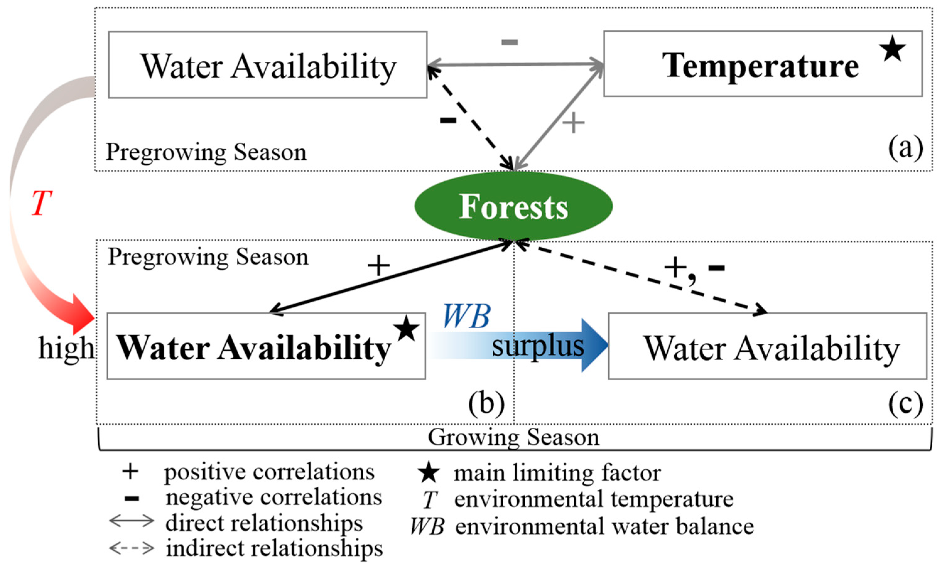
Figure 13.
The underlying mechanism for the positive or negative role of water availability in forest vigor in (a) cold regions during the pregrowing season, (b) warm regions during the pregrowing season or dry regions during the growing season, and (c) wet regions during the growing season. The “−” and “+” represent negative and positive correlations, respectively. The star represents the main limiting factor of forest vigor for different seasons. The dotted and solid lines represent indirect and direct relationships between forest vigor and water availability, respectively. The pregrowing season is January–April, and the growing season is May-September, in China. The temperature and water availability are continuous climatic variables; WB and T are the monthly averaged water balance and temperature during 2001–2015, respectively, which characterize the environmental climate of forests.

Publisher’s Note: MDPI stays neutral with regard to jurisdictional claims in published maps and institutional affiliations. |
© 2020 by the authors. Licensee MDPI, Basel, Switzerland. This article is an open access article distributed under the terms and conditions of the Creative Commons Attribution (CC BY) license (http://creativecommons.org/licenses/by/4.0/).
Share and Cite
MDPI and ACS Style
Luo, H.; Zhou, T.; Liu, X.; Shi, P.; Mao, R.; Zhao, X.; Xu, P.; Yu, P.; Liu, J. Dual Roles of Water Availability in Forest Vigor: A Multiperspective Analysis in China. Remote Sens. 2021, 13, 91. https://doi.org/10.3390/rs13010091
AMA Style
Luo H, Zhou T, Liu X, Shi P, Mao R, Zhao X, Xu P, Yu P, Liu J. Dual Roles of Water Availability in Forest Vigor: A Multiperspective Analysis in China. Remote Sensing. 2021; 13(1):91. https://doi.org/10.3390/rs13010091
Chicago/Turabian StyleLuo, Hui, Tao Zhou, Xia Liu, Peijun Shi, Rui Mao, Xiang Zhao, Peipei Xu, Peixin Yu, and Jiajia Liu. 2021. "Dual Roles of Water Availability in Forest Vigor: A Multiperspective Analysis in China" Remote Sensing 13, no. 1: 91. https://doi.org/10.3390/rs13010091
Note that from the first issue of 2016, this journal uses article numbers instead of page numbers. See further details here.