ECOSTRESS and CIMIS: A Comparison of Potential and Reference Evapotranspiration in Riverside County, California

Abstract

The ECOsystem Spaceborne Thermal Radiometer Experiment on Space Station (ECOSTRESS) provides remotely-sensed estimates of evapotranspiration at 70 m spatial resolution every 1–5 days, sampling across the diurnal cycle. This study, in partnership with an operational water management organization, the Eastern Municipal Water District (EMWD) in Southern California, was conducted to evaluate estimates of evapotranspiration under ideal conditions where water is not limited. EMWD regularly uses a ground-based network of reference evapotranspiration (ET_o) from the California Irrigation Management Information System (CIMIS); yet, there are gaps in spatial coverage and questions of spatial representativeness and consistency. Space-based potential evapotranspiration (PET) estimates, such as those from ECOSTRESS, provide consistent spatial coverage. We compared ECOSTRESS ET_o (estimated from PET) to CIMIS ET_o at five CIMIS sites in Riverside County, California from July 2018–June 2020. We found strong correlations between CIMIS ET_o and ECOSTRESS ET_o across all five sites (R² = 0.89, root mean square error (RMSE) = 0.11 mm hr⁻¹). Both CIMIS and ECOSTRESS ET_o captured similar seasonal patterns through the study period as well as diurnal variability. There were site-specific differences in the relationship between ECOSTRESS AND CIMIS, in part due to spatial heterogeneity around the station site. Consequently, careful examination of landscapes surrounding CIMIS sites must be considered in future comparisons. These results indicate that ECOSTRESS successfully retrieves PET that is comparable to ground-based reference ET, highlighting the potential for providing observation-driven guidance for irrigation management across spatial scales.

1. Introduction

In 2015, more than 94% of California was in a state of severe drought that resulted in a state-wide mandatory reduction on non-agricultural water use by 25% [1]. As a result of this extreme drought period, there was an estimated 564,000 acres of fallowed farmland and impacts on the agricultural economy of California totaling USD 1.8 billion [2]. Extreme drought conditions are expected to worsen due to global climate change [3], stressing the increasing importance on sustainable water management and quantifying water availability and supply.

The Eastern Municipal Water District (EMWD) covers over 1437 km² of California in Southwest Riverside county. This area contains a population of 804,000, with EMWD servicing over 145,000 potable water connections, 237,000 sewer connections and 433 recycled connections. EMWD provides water for both urban and agricultural customers, including 74 agricultural customers with 110 recycled water connections. Recycled water is a key part of EMWD’s water supply portfolio and is currently 100% beneficially reused, with agricultural crop production consuming 67% of this supply. EMWD focuses on responsible use and protection of the natural environment through groundwater management, water use efficiency and various other sustainable practices. Approximately 75% of EMWD’s potable water demand is supplied by imported water from the Metropolitan Water District of Southern California through its Colorado River Aqueduct and its connections to the State Water Project. Approximately 25% of EMWD’s potable water demand is supplied by EMWD groundwater wells.

EMWD has a tiered rate structure based on levels to encourage efficient water use by customer groups and discourage wasteful behaviors. These tiers are applied to a water budget, which is calculated to encourage efficient indoor and outdoor use: (1) the indoor water budget is based on the water volume needed per person per day, (2) the outdoor budget is based on area of landscape, vegetation water use estimated using daily evapotranspiration (ET), and a conservation factor. This outdoor budget calculates actual daily ET, evaporation from the ground and other surfaces and transpiration from plants (Figure 1), using reference evapotranspiration (ET_o) estimates over well-watered standardized pastures, from the California Irrigation Management Information System (CIMIS) weather stations, adjusted by crop coefficients. The CIMIS network is a highly valuable source of information across California, consisting of approximately 155 stations, providing local and highly dense measurements and estimates of weather and reference evapotranspiration [1]. CIMIS provides total precipitation, solar radiation, vapor pressure, air temperature, relative humidity, dew point, wind speed, and soil temperature, as well as a derived hourly ET_o (more frequent estimates are available but not used here). In addition, EMWD uses Spatial CIMIS, which interpolates data from the CIMIS stations with hourly visible National Oceanic and Atmospheric Administration (NOAA) Geostationary Operational Environmental Satellite (GOES) data, especially with regard to incoming solar radiation, to extend ET_o estimated values from the stations to spatial daily ET_o maps (2 km resolution) covering the entire state of California [4]. Although GOES satellite data can provide enhancements and extend the estimates of evapotranspiration [5,6] that are anchored by CIMIS stations [4], its resolution is still relatively coarse, and the interpolation of many critical weather variables such as wind may lead to uncertainty in spatial ET_o for regional to statewide applications.

Evapotranspiration (ET) is a critical component of the hydrologic cycle and represents the greatest data gap in understanding local conditions and demands on water [7]. ET can provide an indication of the amount of consumptive water use from vegetated surfaces, i.e., transpiration, and water loss due to evaporation from water bodies, soils and other surfaces. In addition to ET, potential evapotranspiration (PET) can be used to characterize ET under conditions where water is not limited [8]. This variable can provide insight into atmospheric demands on water and help assess drought conditions. Further, examining the ratio of actual ET and PET can help assess the degree to which a region is water-stressed. This is also known as the Evaporative Stress Index (ESI) [9,10] and has been used as an early warning of drought onset [10].

This study is the first to focus on potential evapotranspiration (PET) from the ECOsystem Spaceborne Thermal Radiometer Experiment on Space Station (ECOSTRESS), a spaceborne instrument launched in June 2018, which acquires thermal data from the International Space Station every 1–5 days (depending on location) at 70 m spatial resolution. Previous work investigating PET derived from other space-based measurements (including NOAA-14 and MODIS) include those applied in the Great Plains [11] and across AmeriFLUX sites in the continental United States [12] at coarser spatial resolutions (1 km). This study is envisioned as the first evaluation of ECOSTRESS PET as well as the first step towards leveraging ECOSTRESS PET for urban water management. To address this objective, we examined ECOSTRESS PET relative to reference ET (ET_o) estimates derived from ground-based CIMIS weather station data through direct comparisons of seasonal patterns and diurnal cycle. The study period spans the full ECOSTRESS data record available at the time of study, from July 2018–June 2020.

2. Methods

2.1. CIMIS ET_o

CIMIS data [1] were downloaded for five stations located in the EMWD area of interest, based in Riverside County in Southern California (Figure 1). These stations measure a suite of meteorological parameters, including solar radiation, air temperature, and relative humidity from which ET_o is derived and made available. This study utilizes the CIMIS ET_o hourly dataset acquired from the period of 15 July 2018 to 10 June 2020. This period corresponds with the timeframe during which ECOSTRESS has been acquiring data.

The hourly ET_o data from CIMIS were derived from a modified Penman equation [13], which is as follows,

$$E{T}_o = c \left[\frac{\Delta }{\Delta + \gamma } \left(Rs \left(1 -\alpha \right) - Rb\right) + \frac{\gamma }{\Delta + \gamma } fu \left(ea - ed\right)\right]$$

(1)

• c = adjustment factor (crop coefficient) (unitless);
• ∆ = slope of saturated vapor pressure at mean air temperature (mbar/degrees C);
• ea = saturated vapor pressure at mean air temperature (mbar);
• ed = actual vapor pressure (mbar);
• fu = wind function (km/day);
• Rs = solar radiation (mm/day);
• Rb = back radiation (mm/day);
• $\gamma$ = psychrometric constant (mbar/degrees C);
• $\alpha$ = albedo (unitless).

This equation [14] calculates ET_o using a modified version of the Penman–Monteith equation, driven by meteorology and the fixed parameters associated with the standardized reference crop, including stomatal and surface resistance, albedo, and height of vegetation. This hypothetical reference crop assumes full shading of the ground, well-watered conditions, and is typically used to represent short green vegetation such as grass or alfalfa. The meteorological input data were measured by CIMIS weather stations, including incoming solar radiation, air temperature, vapor pressure, relative humidity, and wind speed. To inform water demand for crops in the microclimate and under available radiation, the adjustment factor or crop coefficient is applied and varies for each crop type, typically based on empirical data from field measurements.

Although designed as well-maintained pasture sites, many of the CIMIS locations exhibit substantial land cover heterogeneity. Figure 2 provides a snapshot of this heterogeneity, with Station 62—Temecula displaying at least two additional land cover types in addition to the reference field, including water stations and areas with trees. Station 179—Winchester, in addition to the reference field, also shows areas of bare dirt and road. Station 237—Temecula East III is also surrounded by low lying shrubs and bare dirt. Station 239—Hemet location also includes bare dirt, paved road, and different vegetation cover types. Lastly, Station 240—Perris-Menifee shows the reference site surrounded by bare dirt. The site-to-site differences and land cover heterogeneity is taken into account in this study by applying a site-specific calibration, which will be discussed in a following section.

2.2. ECOSTRESS PET

ECOSTRESS is a thermal radiometer that measures thermal infrared radiation (TIR) in five bands ranging from wavelengths of 8 to 12.5 μm and an additional band centered at 1.6 μm for geolocation [2]. Data products most pertinent to this study include the ECOSTRESS Level 3 Evapotranspiration generated using the Priestley–Taylor JPL algorithm [15] and the Level 4 Evaporative Stress Index (ratio of actual evapotranspiration/potential evapotranspiration), which also utilizes PT-JPL and for which calculation of PET is an intermediate product [16,17].

From the Level 4 ESI Data Product, we extracted PET values for the site that came in units of W/m². As part of the ECOSTRESS ESI product, PET is derived from the Priestley and Taylor (1972) [18] equation for calculating ET, which itself is a modified version of the Penman–Monteith (1965) [19] equation. PET, defined below, was extracted as an interim data product from ECOSTRESS ESI:

$$PET= \left[\alpha \frac{\Delta }{\Delta + \gamma } Rn\right]$$

(2)

where R_n represents net radiation, and $\alpha$ is the Priestley and Taylor coefficient, set at 1.26 assuming the maximum rate of evapotranspiration. This equation does not include the parameterization of the stomatal (rs) and aerodynamic resistance (ra) for a crop, which simplifies the equation. ECOSTRESS’ TIR contributes to the PET estimation through the net radiation. Actual ET estimates will approach PET under ideal conditions in which water is not a limiting factor [16,20]. To relate PET in terms of W/m² to CIMIS ET_o in terms of mm hr⁻¹, the following conversion was applied:

$$PET \left(mm/hr\right) = \frac{PET \left(W/m^2\right) \ast 3600 \frac{s}{hr} \ast 1000 \frac{mm}{m}}{\mathsf{\Delta }{H}_{vap}\ast {\rho }_{water}}$$

(3)

where

$$\mathsf{\Delta }{H}_{vap}\left(latent heat of vaporization\right) = 2.45\times {10}^6 J/kg$$

(4)

$${\rho }_{water} = 997 kg/m^3$$

(5)

Sixty ECOSTRESS scenes, spanning from 15 July 2018 to 10 June 2020, were utilized in this study. PET values were extracted from ECOSTRESS ESI pixels over the study area sites (Figure 1). There are two major gaps in the data acquired by ECOSTRESS due to the loss of the primary and redundant sides of the mass storage unit (MSU) from 29 September 2018 to 6 December 2018 and 14 March 2019 to 15 May 2019, respectively. ECOSTRESS data were acquired using the Land Processes Distributed Active Archive Center (LP DAAC) Application for Extracting and Exploring Analysis Ready Samples (AppEEARS) quick subsetting tool [3]. A request over the 5 CIMIS station locations was uploaded to the AppEEARS tool and ECOSTRESS Level 4 Evaporative Stress Index was extracted for these locations and over the ECOSTRESS record. ECOSTRESS PET is necessary for calculating ECOSTRESS Evaporative Stress Index and was therefore available as a secondary product.

2.3. Analysis and Calibration of ECOSTRESS PET to CIMIS ET_o

A calibration step was implemented in the matchup process to account for variability introduced by spatial heterogeneity surrounding each CIMIS site; this was conducted on a site-by-site basis. For each site consisting of N = 50–60, 50% of the samples were randomly selected as training data and used to develop a regression relationship between CIMIS ET_o and ECOSTRESS PET. This linear relationship was used to calibrate ECOSTRESS PET, resulting in an ECOSTRESS ET_o estimate:

$$ECOSTRESS calibrated ETo \left[mm h{r}^{-1}\right]=\frac{ECOSTRESS PET \left[mm h{r}^{-1}\right]- b}{m}$$

(6)

The coefficients (b = intercept and m = slope) were determined by regressing ECOSTRESS PET to CIMIS ET_o at hourly time steps on a site-by-site basis. To evaluate the overall effect of a site-by-site calibration, we pooled all ECOSTRESS ET_o estimates and evaluated the resulting statistical performance of regressing ECOSTRESS ET_o to CIMIS ET_o. Statistics including R², root mean square error (RMSE), normalized root mean square error (nRMSE), and percent bias, were calculated based upon the remaining data (N = 143). There was an improvement in R² from 0.77 (pre-calibration) to 0.81 for Station 62, which exhibited greater spatial heterogeneity than site Station 237, which showed a smaller change in R² = 0.89 to 0.90 (Figure 3). ECOSTRESS ET_o was converted to hourly units and compared with the nearest hourly match from CIMIS ET_o.

2.4. ECOSTRESS and CIMIS ET_o Seasonal and Diurnal Time Series

Data were pooled from all sites for this portion of the study. ET_o was visualized over the full study period and ECOSTRESS data record (up until June 2020) to determine whether ECOSTRESS ET_o could capture recent seasonal scale variability and diurnal variability that were comparable to those of CIMIS ET_o. For recent seasonal variability, this was achieved by conducting weekly composite comparisons for CIMIS ET_o and ECOSTRESS ET_o values, which were then plotted as a time series. For diurnal variability, this study considers ET_o at different times of day during a period identified in the seasonal time series where ET_o remained relatively stable (31 May 2019 to 12 July 2019). During this period, mean values of ECOSTRESS ET_o acquired at different times of the day were overlaid on the mean values of CIMIS ET_o. Standard deviation from ECOSTRESS ET_o acquisitions for each time of day were determined as well.

3. Results

3.1. Matchups ECOSTRESS ET_o and CIMIS ET

The correlation between matchup data (ECOSTRESS PET and CIMIS ET_o) was statistically significant (p < 0.01). After calibration, this study found an overall R² of 0.89 (N = 143), an increase from 0.80 (N = 142) (Figure 4) and an improvement in the RMSE from 0.20 to 0.10 mm hr⁻¹ (

Table 1. Summary statistics for simple linear regression for ECOSTRESS PET (pre-calibrated) and ECOSTRESS ET_o (calibrated), demonstrating improvements in root mean square error (RMSE), normalized root mean square error (nRMSE), and reduction in percent bias.

	R2	MSE	RMSE	nRMSE	Slope	Intercept	%Bias
ECOSTRESS PET	0.80	0.040	0.20	0.20	0.99	0.15	33%
ECOSTRESS ETo	0.89	0.011	0.10	0.11	1.0	0.016	0.0%

). Figure 4 depicts the regression of all points from all five stations. Table 1 summarizes changes in statistics between ECOSTRESS PET and CIMIS ET_o to ECOSTRESS ET_o (calibrated) and CIMIS ET_o. Other changes include an 89% reduction in bias from 0.15 mm hr⁻¹ to 0.016 mm hr⁻¹ and a shift of percent bias from 33% to 0%. The nRMSE was also improved from 20% to 11%.

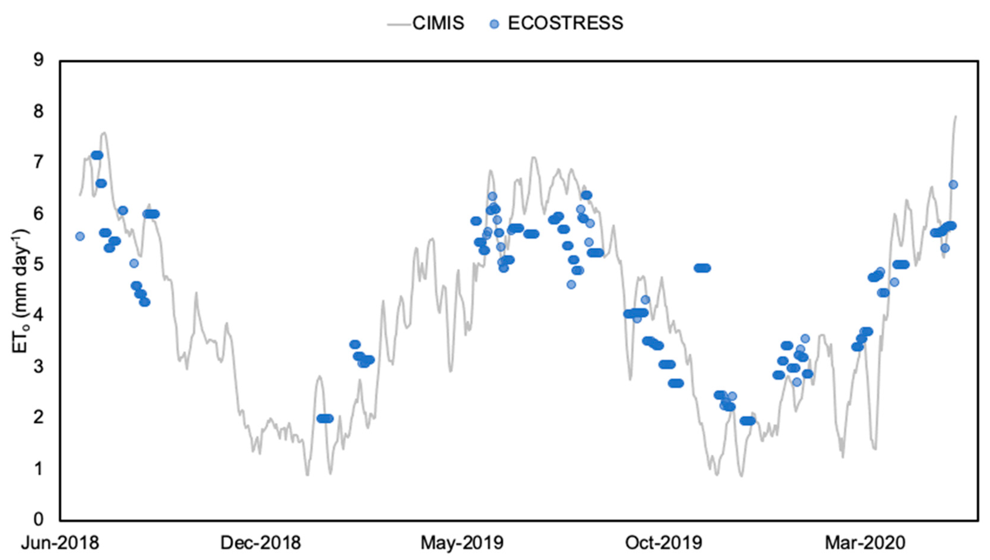
3.2. Seasonal Patterns from July 2018–June 2020

ET_o maximums were observed during summer months (2018, 2019, 2020) and minimums were observed in winter months, though the availability of data during winter months was much more limited (spanning only 2019–2020). In general, this pattern corresponds with expected ET_o seasonal variability of well-watered crops that have a peak growing season during the summer and thus increased ET during this period, and decreased ET during the winter (Figure 5).

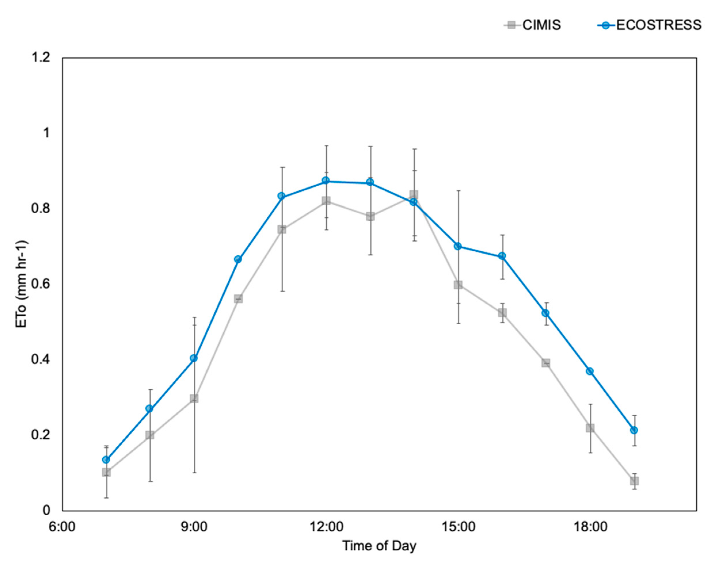
3.3. Diurnal Patterns (31 May 2019–12 July 2019)

At 7:00 AM PT, there was an average CIMIS ET_o value of 0.10 mm hr⁻¹ and a continued increase until a maximum average value of 0.84 mm hr⁻¹ at midday (2:00 PM PT), at which point declines in ET_o were observed until 7:00 PM PT (0.087 mm hr⁻¹) (Figure 6). Both ET_o from ECOSTRESS and CIMIS captured this pattern over the course of the day. ECOSTRESS ET_o means ranged similarly (0.13 mm hr⁻¹) at 7:00 AM PT, peaking at 12:00 PM PT, 0.88 mm hr⁻¹, with a standard deviation ranging from 0.03 to 0.15 mm hr⁻¹.

4. Discussion

4.1. Sources of Uncertainty, Subpixel Contamination and Spatial Heterogeneity

One source of uncertainty was spatial heterogeneity surrounding the CIMIS stations, introduced by mixed land cover and properties and observed in other studies examining PET over heterogeneous areas [12]. This study adapted to these differences by calibrating ECOSTRESS PET to CIMIS ET_o, which allowed for a bias adjustment (Figure 2) and is reflected in Figure 3 and summarized in Table 1. Future work may consider factoring land cover characteristics into optimal pixel selection within a scene, particularly where mixed use (built and natural environment) is present. In many cases, the size of the reference fields that the CIMIS stations represent are smaller than one ECOSTRESS pixel (70 × 70 m), which can contribute to pixel contamination due to surrounding landscapes that affect the estimations of PET, as shown in the site maps in Figure 2.

4.2. Differences in Spatial Scales and Changing Ground Conditions

One of the primary differences between ECOSTRESS and CIMIS are spatial sampling scales, where ECOSTRESS samples every 1–5 days at 70 m spatial resolution, and CIMIS sites are acquiring meteorological data at point-scale at well-watered plots with reference crop cover to ensure microclimate conditions are driven by land surface characteristics. CIMIS ET_o calculations are based off of mean air temperature, net radiation, and wind measurements. In semi-arid regions, there is the potential for readings to be inaccurate due to high magnitude of ground heat flux impacting longwave radiation measurements, as well as strong biotic, or atmospherically decoupled, control over ET [12,21]. In addition, changes in field status and maintenance could influence the ET_o estimates, particularly at the CIMIS station scale. Furthermore, ECOSTRESS PET utilizes satellite estimates of albedo of the area of interest from MODIS [21], which can vary depending on MODIS availability and can be influenced by local albedo conditions of the field site. This study observed some range in statistics site-to-site, which was likely due to spatial heterogeneity around each station (Figure 3). Note that Temecula East III 237 has a more homogeneous footprint within the ECOSTRESS pixel with more chaparral and brush coverage, whereas Temecula 62 has three different land covers present with a water storage unit laden with pavement and concrete, a dark-colored dirt plot with trees, and a light-colored dirt plot with trees. A visual inspection of historic Google Earth images for the sites showed substantial changes in land cover conditions over our period of study, such that selection of consistently homogenous reference sites over Riverside County was not immediately feasible. Despite this variability, statistics across all five sites indicated a strong correlation between the two datasets (R² = 0.89 after calibration, and R² = 0.80 prior to calibration). The Normalized Difference Vegetation Index (NDVI), defined as the ratio of reflected near-infrared light to reflected visible light, is used as an indicator of plant greenness and health, and could potentially be used to help account for recent conditions of the reference site in future work.

4.3. Differences in PET Models

There are a variety of methods to calculate potential evapotranspiration; however, the three most popular methods are the Thornthwaite (temperature-based), Priestley–Taylor (radiation-based) and Penman–Monteith (combination-based) models [8]. Of these three methods, Priestley–Taylor and Penman–Monteith are most similar to one another because the dominant term in the PET calculation is the net radiation (Rn) term, relative to local variables such as air temperature, wind speed and vapor pressure deficit [8]. In a comparison study of potential evaporation across the globe with eddy covariance sites, Palmer et al. [20] and Maes et al. [22] reported that a Priestly–Taylor model with a biome specified albedo consistently performed better than Penman, Penman–Monteith, or any temperature-based models. This difference may in part be due to how the Penman–Monteith models utilize a constant for unstressed stomatal conductance [22]. The Priestley–Taylor method contains an implicit assumption of the wind speed effects on PET being addressed by the albedo term [22], which could also introduce uncertainty in PET estimates. However, it has been shown in other studies that the vast spatial heterogeneity of stomatal resistance and other small-scale Penman–Monteith factors may be adequately represented by the Priestley–Taylor method at larger scales as land surface complexity increases greatly [11,23,24]. Overall, there seems to be agreement that the Priestley–Taylor method is well suited for large-scale remote sensing studies, and further, demonstrates satisfactory performance when compared to other PET estimation models.

In this study, ECOSTRESS ET_o values were comparable to ground-based estimates of ET_o (R² = 0.89, RMSE = 0.10 mm hr⁻¹). Similarly, in 2008, one study evaluated a MODIS-based Priestly–Taylor PET product evaluation at the point-scale compared to daily PET calculations from MODIS to four FLUXNET eddy covariance station locations [12]. The variable sampling at the daily temporal scale with modeled and observed PET used a modified Priestley–Taylor parameterization to improve their results over observations across the year of 1997 (R² = 0.90) [11]. Further, He et al. [25] employed a satellite-based surface energy balance approach (METRIC) to compare field scale crop ET_o to actual ET (R² = 0.74; RMSE = 0.14 mm day⁻¹) over an almond orchard using Landsat observations [25], which matched closely for the year of 2004 (R² = 0.87; RMSE = 1.81 mm day⁻¹; bias = −0.70 mm day⁻¹). With respect to temporal sampling, ECOSTRESS PET has five times the observations in half the time window and a better agreement of the data across the year (Figure 6), falling within the min/max range of CIMIS ET_o values acquired over the same period. This study and its subsequent results have important implications for water utility districts, individual farmers, and others in the water resource management space. While R² values appeared to be comparable across these studies, it should be noted that this work was examining ECOSTRESS PET relative to CIMIS ET_o, not ground-based estimates of PET, as the ultimate goal was to demonstrate comparable estimates of ECOSTRESS PET to support future consideration of this product as an enhancement of existing CIMIS ET_o or spatial CIMIS ET_o estimates.

4.4. Applications of Water Management

On average, 53% of all potable water used at residential properties in California is used to irrigate ornamental landscapes [26]. About 47% of all homes are over-irrigating, which can be due to irrigation system inefficiencies and failure to change watering schedules to match actual evapotranspiration demands. EMWD is exploring methods and new datasets, such as ECOSTRESS, to better understand consumptive water needs, with the goal of improving water conservation and efficiency in water usages. The backdrop of these goals is the need to meet the future water demands of a growing population, reducing wasted water and energy caused by excessive landscape irrigation, and better communicating to customers the actual amount of water needed to maintain healthy plant material at their properties. These progressive methods will help in combatting the effects of anthropogenic warming, which is expected to intensify drought severity in California [3].

Derived primarily from remote sensing observations with moderate resolution, PET can potentially serve as a proxy for spatially explicit and time varying water demand estimates, and thus overcome the uncertainties due to spatial interpolation of CIMIS ET_o. This validation study provides the first step towards this by evaluating ECOSTRESS PET relative to ET_o from CIMIS sites, with greater spatial coverage, better spatial resolution than spatial CIMIS (2 km) [4] and comparable estimates in value. While we note various sources of variability in ECOSTRESS PET and CIMIS ET_o, minor calibration of these measurements can be implemented to adjust for site-to-site biases that may arise, likely due to uncertainties as described previously. It is important to note that while ECOSTRESS and many other space-based assessments of ET provide good spatial coverage, CIMIS ET_o provides high frequency temporal measurements, demonstrating the high complementarity between the two datasets. Furthermore, ECOSTRESS is unique in its variable overpass and sampling times, which can provide insights into ET conditions across broader spatial scales and at different times of the day. Enhanced evapotranspiration metrics can improve how Californians use water during drought conditions and even aid in monitoring drought. Creating a higher resolution ET data product for relevant stakeholders will be vital in assessing vegetation health, improving irrigation methods, and conserving water.

5. Conclusions

Results show good agreement between ECOSTRESS ET_o and CIMIS ET_o (R² = 0.89, RMSE = 0.11 mm hr^-1) with possibilities to strengthen this agreement by considering sources of spatial variability. Primary sources of uncertainty include landscape heterogeneity among the reference station sites, differences in spatial footprints of ECOSTRESS pixels and CIMIS stations, CIMIS station discrepancies in readings due to ground conditions (changing mean air temperature due to advection), and inherent differences arising from the different models being implemented for estimation of ET_o and PET. Future considerations may consider use of NDVI to help locate nearby homogeneous sites to help optimize pixel selection for ECOSTRESS. However, these data show that ECOSTRESS PET is comparable to CIMIS reference ET, across spatial scales enabled by ECOSTRESS measurements. This has significant implications for water utilities such as EMWD, agricultural managers, and other water management entities across the state, representing an opportunity to supplement CIMIS ET_o site estimates with an independent estimate of PET conditions with greater spatial coverage at 70 m spatial resolution.

References

1. Cody, B.A. California Drought: Water Supply and Conveyance Issues; Congressional Research Service: 101 Independence Ave, SE; Library of Congress: Washington, DC, USA, 2015. [Google Scholar]
2. Howitt, R.; MacEwan, D.; Medellín-Azuara, J. Economic Analysis of the 2015 Drought for California Agriculture; Agricultural Issues Center University of California One Shields Avenue: Davis, CA, USA, 2015. [Google Scholar]
3. Williams, A.P.; Seager, R.; Abatzoglou, J.T.; Cook, B.I.; Smerdon, J.E.; Cook, E.R. Contribution of anthropogenic warming to California drought during 2012–2014. Geophys. Res. Lett. 2015, 42, 6819–6828. [Google Scholar] [CrossRef] [Green Version]
4. Hart, Q.J.; Brugnach, M.; Temesgen, B.; Rueda, C.; Ustin, S.L.; Frame, K. Daily reference evapotranspiration for California using satellite imagery and weather station measurement interpolation. Civ. Eng. Environ. Syst. 2009, 26, 19–33. [Google Scholar] [CrossRef]
5. Cahn, M.; Hartz, T.; Smith, R.; Noel, B.; Johnson, L.; Melton, F. CropManage: An online decision support tool for irrigation and nutrient management. In Proceedings of the Western Nutrient Management Conference, Reno, NV, USA, 5–6 March 2015; Volume 11. [Google Scholar]
6. Melton, F.S.; Johnson, L.F.; Lund, C.P.; Pierce, L.L.; Michaelis, A.R.; Hiatt, S.H.; Guzman, A.; Adhikari, D.D.; Purdy, A.J.; Rosevelt, C.; et al. Satellite Irrigation Management Support with the Terrestrial Observation and Prediction System: A Framework for Integration of Satellite and Surface Observations to Support Improvements in Agricultural Water Resource Management. IEEE J. Sel. Top. Appl. Earth Obs. Remote Sens. 2012, 5, 1709–1721. [Google Scholar] [CrossRef]
7. Melton, F.S.; Allen, R.G.; Anderson, M.C.; Bolten, J.; Cestti, R.; Dunsmoor, L.; Erickson, T.; Fisher, J.; Hain, C.R.; Harshadeep, N.; et al. Evapotranspiration Mapping for Water Security: Recommendations and Requirements. In Proceedings of the 2015 Workshop on ET Mapping for Water Security Workshop, Washington, DC, USA, 15–17 September 2015. [Google Scholar]
8. Fisher, J.B.; Whittaker, R.J.; Malhi, Y. ET come home: Potential evapotranspiration in geographical ecology. Glob. Ecol. Biogeogr. 2011, 20, 1–18. [Google Scholar] [CrossRef]
9. Anderson, M.C.; Zolin, C.A.; Hain, C.R.; Semmens, K.; Tugrul Yilmaz, M.; Gao, F. Comparison of satellite-derived LAI and precipitation anomalies over Brazil with a thermal infrared-based Evaporative Stress Index for 2003–2013. J. Hydrol. 2015, 526, 287–302. [Google Scholar] [CrossRef] [Green Version]
10. Otkin, J.A.; Anderson, M.C.; Hain, C.; Mladenova, I.E.; Basara, J.B.; Svoboda, M. Examining rapid onset drought development using the thermal infrared-based evaporative stress index. J. Hydrometeorol. 2013, 14, 1057–1074. [Google Scholar] [CrossRef]
11. Jiang, L.; Islam, S. Estimation of surface evaporation map over southern Great Plains using remote sensing data. Water Resour. Res. 2001, 37, 329–340. [Google Scholar] [CrossRef] [Green Version]
12. Kim, J.; Hogue, T.S. Evaluation of a MODIS-based potential evapotranspiration product at the point scale. J. Hydrometeorol. 2008, 9, 444–460. [Google Scholar] [CrossRef]
13. Doorenbos, J.; Pruitt, W.O. Guidelines for Predicting Crop Water Requirements; FAO Irrig. Drain. Pap.; FAO: Rome, Italy, 1977; Volume 24, p. 144. [Google Scholar]
14. Batchelor, C.H. The accuracy of evapotranspiration estimated with the FAO modified penman equation. Irrig. Sci. 1984, 5, 223–233. [Google Scholar] [CrossRef]
15. Fisher, J.B. Level-3 Evapotranspiration L3(ET_PT-JPL) Algorithm Theoretical Basis Document (ECOSTRESS); Jet Propuslion Laboratory, California Institute of Technology: Pasadena, CA, USA, 2018; Volume 3. [Google Scholar]
16. Fisher, J.B. Level-4 Evaporative Stress Index L4(ESI_PT-JPL) Algorithm Theoretical Basis Document (ECOSTRESS); Jet Propulsion Laboratory, California Institute of Technology: Pasadena, CA, USA, 2018; Volume 4. [Google Scholar]
17. Fisher, J.B.; Tu, K.P.; Baldocchi, D.D. Global estimates of the land–atmosphere water flux based on monthly AVHRR and ISLSCP-II data, validated at 16 FLUXNET sites. Remote Sens. Environ. 2008, 112, 901–919. [Google Scholar] [CrossRef]
18. PRIESTLEY, C.H.B.; TAYLOR, R.J. On the Assessment of Surface Heat Flux and Evaporation Using Large-Scale Parameters. Mon. Weather Rev. 1972, 100, 81–92. [Google Scholar] [CrossRef]
19. Penman, H.; Monteith, J. Chapter 2—FAO Penman-Monteith Equation. Available online: http://www.fao.org/3/x0490E/x0490e06.htm (accessed on 6 October 2020).
20. Palmer, C.; Fisher, J.B.; Mallick, K.; Lee, J. The Potential of Potential Evapotranspiration. Available online: https://ui.adsabs.harvard.edu/abs/2012AGUFM.H32B..03P/abstract (accessed on 9 October 2020).
21. Fisher, J.B.; Lee, B.; Purdy, A.J.; Halverson, G.H.; Dohlen, M.B.; Cawse-Nicholson, K.; Wang, A.; Anderson, R.G.; Aragon, B.; Arain, M.A.; et al. ECOSTRESS: NASA’s Next Generation Mission to Measure Evapotranspiration From the International Space Station. Water Resour. Res. 2020, 56. [Google Scholar] [CrossRef]
22. Maes, W.H.; Gentine, P.; Verhoest, N.E.C.; Miralles, D.G. Potential evaporation at eddy-covariance sites across the globe. Hydrol. Earth Syst. Sci. 2019, 23, 925–948. [Google Scholar] [CrossRef] [Green Version]
23. Brutsaert, W.; Stricker, H. An advection-aridity approach to estimate actual regional evapotranspiration. Water Resour. Res. 1979, 15, 443–450. [Google Scholar] [CrossRef]
24. Shuttleworth, W.J. Evaporation Models in Hydrology. In Land Surface Evaporation; Springer: New York, NY, USA, 1991; pp. 93–120. [Google Scholar]
25. He, R.; Jin, Y.; Kandelous, M.; Zaccaria, D.; Sanden, B.; Snyder, R.; Jiang, J.; Hopmans, J. Evapotranspiration Estimate over an Almond Orchard Using Landsat Satellite Observations. Remote Sens. 2017, 9, 436. [Google Scholar] [CrossRef] [Green Version]
26. DeOreo, W.B.; Mayer, P.W.; Martien, L.; Hayden, M.; Funk, A.; Kramer, M.; Davis, R.; Henderson, J.; Raucher, B.; Gleick, P.; et al. California Single Family Water Use Efficiency Study; Aquacraft Water Engineering and Management: Boulder, CO, USA, 2011; pp. 1–391. [Google Scholar]
Figure 1. California Irrigation Management Information System (CIMIS) station locations used by Eastern Municipal Water District in Southwest Riverside County, CA. Black triangles represent 155 CIMIS stations in California; red circles represent the stations used in this study.
Remotesensing 12 04126 g001
Figure 2. CIMIS stations in the Eastern Municipal Water District (EMWD) purview, located in heterogeneous environments. (A) Station 239/Hemet; (B) Station 240/Perris–Menifee; (C) Station 179/Winchester; (D) Station 62/Temecula; (E) Station 237/Temecula East III.
Remotesensing 12 04126 g002
Figure 3. CIMIS sites (A,B) exhibit varying levels of spatial heterogeneity, with examples shown here. Station 237, while showing paved areas, is largely vegetation and some bare dirt, whereas Station 62 is within 50 m of a water tower. (C,D) exemplify the ECOsystem Spaceborne Thermal Radiometer Experiment on Space Station (ECOSTRESS) potential evapotranspiration (PET) (pre-calibrated; gray squares) and ETo (calibrated; blue circles) correlated to CIMIS reference evapotranspiration (ETo). Stations 237 and 62 correspond with Figure 2A,B and Figure 2B,D respectively.
Remotesensing 12 04126 g003
Figure 4. Linear regression was applied to the test data across all five stations (N = 143), with an overall R2 of 0.89.
Remotesensing 12 04126 g004
Figure 5. Seasonal time series using weekly composites of ECOSTRESS ETo (blue circles) and CIMIS ETo (grey line).
Remotesensing 12 04126 g005
Figure 6. ECOSTRESS ETo (blue circles) and CIMIS ETo (grey squares) exhibit diurnal variability in reference evapotranspiration that peaks during midday hours, with data aggregated for the period of 5/31/2019 to 7/12/2019, over all five stations, and shown over the diurnal cycle. Error bars represent standard deviation of values.
Remotesensing 12 04126 g006