UAV-Derived Multispectral Bathymetry

1
GEOCOSTE, Via Corsi, 19, 50141 Firenze, Italy
2
INGV, Via Cesare Battisti, 53, 56125 Pisa, Italy
*
Author to whom correspondence should be addressed.
Remote Sens. 2020, 12(23), 3897; https://doi.org/10.3390/rs12233897
Submission received: 18 October 2020
/
Revised: 23 November 2020
/
Accepted: 23 November 2020
/
Published: 27 November 2020
(This article belongs to the Special Issue UAV Application for Monitoring Coastal Morphology)
Abstract
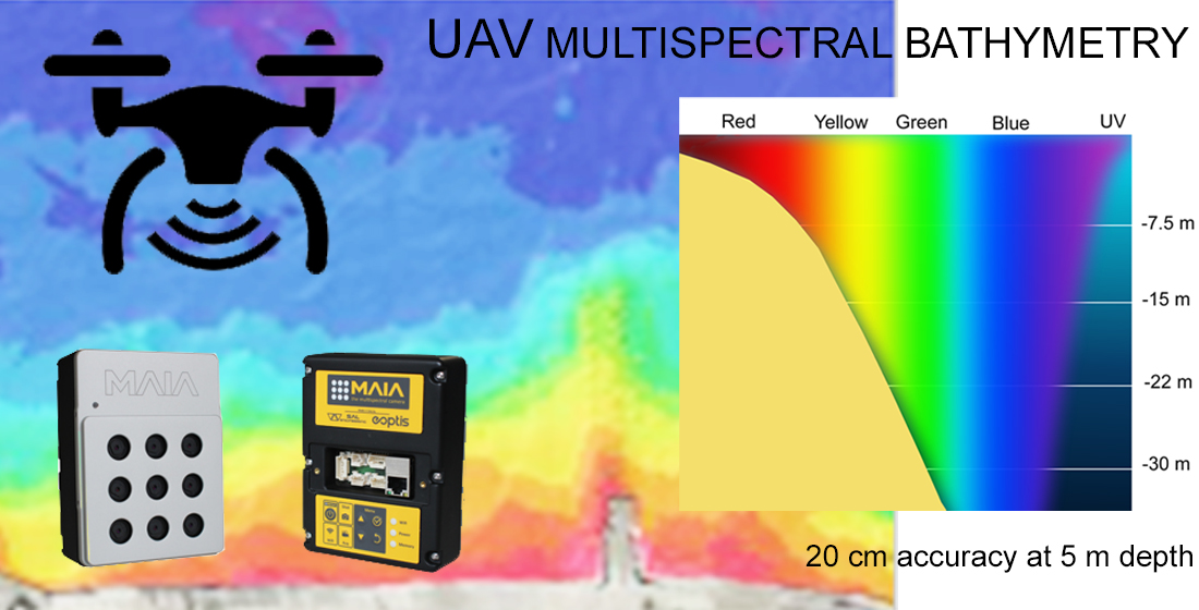
:Bathymetry is considered an important component in marine applications as several coastal erosion monitoring and engineering projects are carried out in this field. It is traditionally acquired via shipboard echo sounding, but nowadays, multispectral satellite imagery is also commonly applied using different remote sensing-based algorithms. Satellite-Derived Bathymetry (SDB) relates the surface reflectance of shallow coastal waters to the depth of the water column. The present study shows the results of the application of Stumpf and Lyzenga algorithms to derive the bathymetry for a small area using an Unmanned Aerial Vehicle (UAV), also known as a drone, equipped with a multispectral camera acquiring images in the same WorldView-2 satellite sensor spectral bands. A hydrographic Multibeam Echosounder survey was performed in the same period in order to validate the method’s results and accuracy. The study area was approximately 0.5 km2 and located in Tuscany (Italy). Because of the high percentage of water in the images, a new methodology was also implemented for producing a georeferenced orthophoto mosaic. UAV multispectral images were processed to retrieve bathymetric data for testing different band combinations and evaluating the accuracy as a function of the density and quantity of sea bottom control points. Our results indicate that UAV-Derived Bathymetry (UDB) permits an accuracy of about 20 cm to be obtained in bathymetric mapping in shallow waters, minimizing operative expenses and giving the possibility to program a coastal monitoring surveying activity. The full sea bottom coverage obtained using this methodology permits detailed Digital Elevation Models (DEMs) comparable to a Multibeam Echosounder survey, and can also be applied in very shallow waters, where the traditional hydrographic approach requires hard fieldwork and presents operational limits.

1. Introduction
Worldwide coastal areas are dynamic environments, constantly evolving and being reshaped due to natural processes [1] and human activities [2]. The factors responsible for their change may be described as geological and geomorphological, hydrodynamic, biological, climatic, and anthropogenic [3]. Taking place over a range of timescales, the interaction of these factors causes dynamic coastal rebuilding, referred to as coastal morphodynamics. The coastal system is also a dynamic complex of sensitive elements and typically responds in a nonlinear morphological manner [4]. Coastal environments host key infrastructures and ecosystems. Additionally, about 40% of the world’s global population live within 100 km of the coast and around 10% live in areas that are less than 10 m above sea level [5], so these environments represent a critical part of the economies of many nations bordering the sea, particularly subsistence economies [6].
Monitoring, evaluating, and reporting activities and adaptive management approaches are widely recognized as fundamental components of any effective coastal protection policy [7]. Implemented management measures are also important in terms of understanding how planning and decision-making in adaptive maritime spatial planning may be improved [8]. Coastal zone monitoring is an essential process for sustainable coastal management and environmental protection. Regular monitoring, the assessment of coastal morphodynamics, and identification of the processes influencing sediment transport, erosion, or accretion are thus increasingly important for developing a better understanding of changes and evolutionary trends in these particular systems [9] and have important roles in their dynamic behavior [10,11]. High spatial resolution (<1 m) remotely sensed images and Digital Elevation Models (DEMs) are widely used in marine environment monitoring [12] and are important tools for improving Integrated Coastal Zone Management (ICZM) studies.
Nowadays, three-dimensional data mainly acquired by Laser Imaging Detection and Ranging (LiDAR) [13] and with Structure from Motion (SfM) [14] photogrammetry applied to photographs captured from unmanned aerial vehicles or systems (UAVs and UASs, respectively) [15,16,17] are the most frequently used aerial survey technologies for emerged beaches and coasts [18].
Since at least the 1980s, the bathymetric data demand has also increased considerably due to the upgrade of marine chart navigation, exploration of marine resources, environmental protection, and coastal erosion or defense projects [19]. Bathymetry is one of the key factors used by scientists, hydrographers, and decision-makers operating in coastal zones [20] and it provides useful information on the ecological and geomorphological processes. Accurate and reliable bathymetry information is important for coastal erosion studies, maritime navigation, the mapping and monitoring of benthic habits, dredging planning, and coastal management [21]. Bathymetric surveys are generally performed with Single beam Echosounder (SbEs) and Multibeam Echosounder (MbEs) technology, to obtain more detail [22,23]. Such an approach requires treacherous work in the field and is extremely expensive and laborious, referring to shallow and wide water areas [24]. An MbEs survey of 1 km2 in a shallow water area would take approximately 10 operative days and cost up to EUR 10.000. Moreover, there are complications regarding survey vessel mob/demob, permits, and sea conditions. At less than a c.a. 2 m depth, an MbEs survey is also limited [25] because of its characteristics and usually, the bathymetry is carried out with a small boat equipped with an SbEs, an aquatic unmanned surface vehicle [26], or a GPS-RTK topographic survey down to a c.a. 1 m depth near the shoreline.
Airborne Laser Bathymetry (ALB), which is an active remote sensing technique for capturing shallow water areas using green laser light, has rapidly evolved in recent years [27]. ALB and high-resolution satellite images have been increasingly applied for coastal monitoring and bathymetric mapping, even though the traditional approach is a hydrographic survey with echo sounders. ALB mainly involves airborne acquisition and can measure topography in addition to bathymetry.
Satellite-Derived Bathymetry (SDB) conducted through multispectral satellite image processing is the most recently developed method for surveying shallow waters and has proven itself as a useful reconnaissance and planning tool for ocean mapping, although it provides bathymetry products at a coarser spatial resolution compared to traditional acoustic surveying (e.g., MbEs) or ALB [28]. The problem of estimating water depths from remote sensing data has a relatively long history. The first application was conducted in 1975, when the sea bottom topography in the Bahamas was calculated to a depth of about 20 m by NASA using Landsat 1 satellite multispectral images. Since the early 2000s, physics-based radiative transfer models have become a popular means of determining the bathymetry of coastal regions using high-resolution satellite imagery. SDB has provided a cost- and time-effective solution for the determination of the bottom morphology in shallow water areas [29,30] and the accuracy is improved, especially with the use of recent high-resolution satellite sensors, such as DigitalGlobe’s WorldView-2 and -3 (WV2-3) and Quick Bird [31,32]. WorldView-2 has a resolution of 50 cm (panchromatic) and 2 m (8 multispectral bands). In addition to the four standard bands (blue, green, red, and near-infrared), the imagery also contains four colors (red edge, coastal, yellow, and near-infrared 2). In the last five years, Sentinel-2A/B data from the Copernicus program have also become available. These data are free, in contrast to data from commercial satellites, and the results obtained in the SDB field are promising, especially over large areas [33,34].
SDB methods can be grouped into empirical, semi-analytic, and physical-based approaches [35]. The methodology relates the surface reflectance of shallow coastal waters to the depth of the water column. Different visible wavelengths of electromagnetic radiation can penetrate the water column and can be reflected from the sea bottom at different depths, which is the premise for bathymetry-derived multispectral imagery [36]. Light with longer wavelengths is absorbed more quickly than that with shorter wavelengths. Because of this, the higher energy light with short wavelengths, such as blue, is able to penetrate more deeply. The use of passive sensor data in bathymetry is also affected by water turbidity and bottom signals [37] and satellite images are complicated by atmospheric correction because the wavelengths measured at the top-of-atmosphere (TOA) are influenced by the composition of the atmosphere [38].
Many empirical models have been studied for water depth estimation relating to image pixel values with the bottom depth. One of the most used algorithms was proposed by Lyzenga [39,40,41], and the model was based on the radiance model for water, whereby the radiance received could be calculated as a linear function of the reflected radiance and an exponential function of the water depth. Jupp [42] introduced a method for first determining the depth of penetration (DOP) zones for every band and then for calibrating depths within these zones. Stumpf [43] proposed an algorithm using a log-band ratio of reflectance, contrary to the standard linear transform algorithm, reducing the number of parameters in the equation. The most accurate results gathered for bathymetric mapping for satellite multispectral approaches show, when water depths are within 15 m, a relative depth error of approximately 10% [44] or even better, as in recent studies [20,34]. Multispectral airborne data have also been used to map bathymetry in rivers [45].
In the last ten years, the rapid development and growth of UAVs as remote sensing platforms, as well as advances in the miniaturization of instrumentation and data systems, have resulted in an increasing uptake of this technology in environmental and remote sensing science communities [46]. Nowadays, UAVs are the fastest monitoring systems for terrestrial and emerged coastal areas [47,48,49] and the elaboration of ortho-images represents a useful tool for the study of the territory and environment [50]. Researchers have proposed UAV-based solutions for almost any conceivable problem, but the greatest impact will likely be in applications that exploit the unique advantages of the technology: work in dangerous or difficult-to-access areas; high spatial resolution and/or frequent measurements of environmental phenomena; the deployment of novel sensing technology over small to moderate spatial scales [51]. The main advantages of this technology are its high accuracy, full coverage of the surveyed area, and high degree of operational flexibility, as well as the possibility to deliver high temporal and spatial resolution image information in a short period of time [52]. Drones are now a valuable source of data for mapping and 3D modeling and low-cost and are easily transportable carriers able to collect data in a short period of time. The main fields of application are precision agricultural analysis, archaeological surveying, and land topography or coastal monitoring [53].
Several scientific studies have assessed the accuracy of UAV-borne remote sensing for seabed mapping or derivation of the water depth using different approaches and methodologies, such as small topo-bathymetric laser profilers [54,55], SfM and photogrammetry [56,57,58,59], RGB images [60,61,62], video techniques or fluid lensing technology [63,64], and, in gravel bed clear river water, multispectral linear transform models [65,66] or hyperspectral data [67]. All of these methods have weaknesses and strengths in bathymetric applications with a low DEM accuracy and results that cannot be used to obtain a detailed 3D terrain model are useful for coastal monitoring programs or marine engineering projects.
Over the last few years, small drones, in combination with cost-efficient and lightweight RGB cameras, have become a standard tool for typical photogrammetric tasks. Multispectral sensors, in contrast, have long been too heavy for use on these platforms, but recently, complex high-end and lightweight multispectral sensors for UAV have become commercially available [68].
In this article, we investigate the capabilities and discuss promising results obtained from a field test of one of these commercial sensors, mounted on a drone, for its applicability to hydrographic tasks. This manuscript is an extended conference paper [69], where a new methodology for remote sensing bathymetry is presented using a UAV equipped with a professional multispectral camera. Images were processed by applying algorithms for remote sensing normally used in Satellite-Derived Bathymetry. In this paper, the introduction, discussion, and conclusions have been improved and a detailed review of UAV bathymetry research has been incorporated. A deeper analysis of the literature review in the form of the state of the has also been added, in order to compare the results with global literature. The study was also implemented by using Lyzenga’s method. A side-by-side analysis of bathymetry derived from these new methodologies, UAV-Derived Bathymetry (UDB), and satellite images are given and the depth accuracy was verified through a comparison with an in situ field hydrographic survey. The scope of this study was to undertake a first evaluation of the potential of UDB for coastal monitoring activity and evaluate whether images acquired by a low-cost UAV and multispectral camera could become useful tools in supporting coastal management and studies.
2. Materials and Methods
2.1. Area of Study
For this research, an area of about 400 × 300 m was selected. The area is located on the coast on the Tyrrhenian sea in the south of San Vincenzo town (LI) in Italy, along a 9 km sand beach (Figure 1) characterized by cusps, sandbars, and some beach rock outcrops and extending from the shoreline to about the beginning of the Posidonia Oceanica edge. The internal limit of Posidonia Oceanica meadow, which is a seagrass species that is endemic to the Mediterranean Sea, is located at about a −10 m depth. Several morphological data are available for this area and were mainly deduced from erosion monitoring studies conducted by the local municipality and the University of Florence. Moreover, in the same period in which we needed to test the methodology, we had to perform a hydrographic survey for a beach nourishment project.
The coordinate reference system used in this work was WGS84/UTM 32 North and the Military Geographic Institute (IGM) was used as the vertical national datum. This geodetical reference system was used for all of the surveys and image processing conducted in the study.
2.2. Empirical Satellite-Derived Bathymetry (SDB) Models
The study was conducted using two algorithms from the literature, which had previously only been applied to satellite imagery. They were applied to UAV multispectral imagery, without modifying or implementing the equations.
The Stumpf Relative Water Depth algorithm (RWD) linearizes the relationship between band spectral values and the sea bottom depth with a log-transformation and uses a log-band ratio to reduce the number of parameters in the equation and generate depth classes of relative water depth which can then be rescaled to real bathymetric data by using real depth values. In this way, the error due to the variation of the radiation in the atmosphere and the water column is reduced and is less sensitive to sea bottom variation [70]. The bottom albedo-independent nature of the algorithm means that seafloor covered with dark seagrass or bright sand is shown to be at the same depth when they are at the same depth.
This model applies the fundamental principle that every band has a different level of water body absorption. The RWD algorithm is described in Equation (1):
where Z is the derived depth (m), m1 is a tunable constant to scale the ratio to depth, and n is a fixed constant for all areas. A positive large number is chosen to keep the ratio positive for any reflectance value. m0 is the offset for a depth of 0 m (Z = 0) and Rw is the observed radiance for bands λi and λj.
The Stumpf model was processed using the ENVI™ 5 suite.
By also utilizing the newly available yellow and coastal-blue spectral bands present in satellite and UAV multispectral sensors, an optimal band ratio analysis (OBRA) method was tested, which compared different pairs of wavelengths (coastal-blue/green and yellow/green) in order to determine the best solution for the study area. These ratio combination results were compared with the more traditional blue/green and green/red combinations. Initially, the water depth results were relative, since they do not depict absolute depths (the results are scaled from zero to one). The intent of these results is to provide a general feel for the bathymetry; they are not to be used for navigational purposes. Calibration with real sea bottom depth values was then requested to scale the previous values, in order to produce a bathymetric map. In our elaboration, a density slice at spectral reflectance intervals was computed and calibrated with real survey depths, testing a different number of Sea Bottom Control Points (SBCPs).
The equations developed by Lyzenga are based on the fact that sea-surface radiation is approximately a linear function of bottom reflectance and an exponential function of water depth. He used an albedo-independent method to derive a bathymetric map from a multispectral scene. The method considers the exponential relationship of light attenuation through a column of water to develop a linear transformation function that relates the observed radiance to the water depth. Lyzenga attempted to account for variability in bottom type by using multiple spectral bands and a rotational matrix. Theoretically, the numbers of significantly different bottom types and water masses for which this algorithm accounts are directly proportional to the number of bands used, implying that Worldview-2 imagery, with 8 bands, should produce more accurate results over heterogeneous waters than conventional multispectral satellites.
Equation (2) is the algorithm for the log-linear inversion model:
where Z is the derived depth (m); m0, mi (i = 0,1, …, N) are the constant coefficients for N spectral bands; L(λi) is the remote sensing radiance after atmospheric and sun-glint corrections for spectral band λi; L∞(λi) is the deep-water radiance for spectral band λi. The constants are usually determined by a multiple linear regression. In the case of shallow water, the radiance observed by the satellite consists of four components: atmospheric scattering; surface reflection, in-water volume scattering; bottom reflection.
In Lyzenga’s 1981 correction method, sea-surface or atmospheric scattering is implicitly assumed to be homogeneous over the target area and in Lyzenga’s 2006 model, they are expected to vary from pixel to pixel and variations are linearly related to the radiance of the near-infrared band. ArcGIS and ENVI™ 5 were also used for data processing.
2.3. Satellite Data Processing
For the Satellite-Derived Bathymetry (SDB) remote sensing processing, we used a WV2 image dataset (Figure 2) acquired on 13 December 2016 (panchromatic 50 cm res + 8 multispectral bands 2 m res).
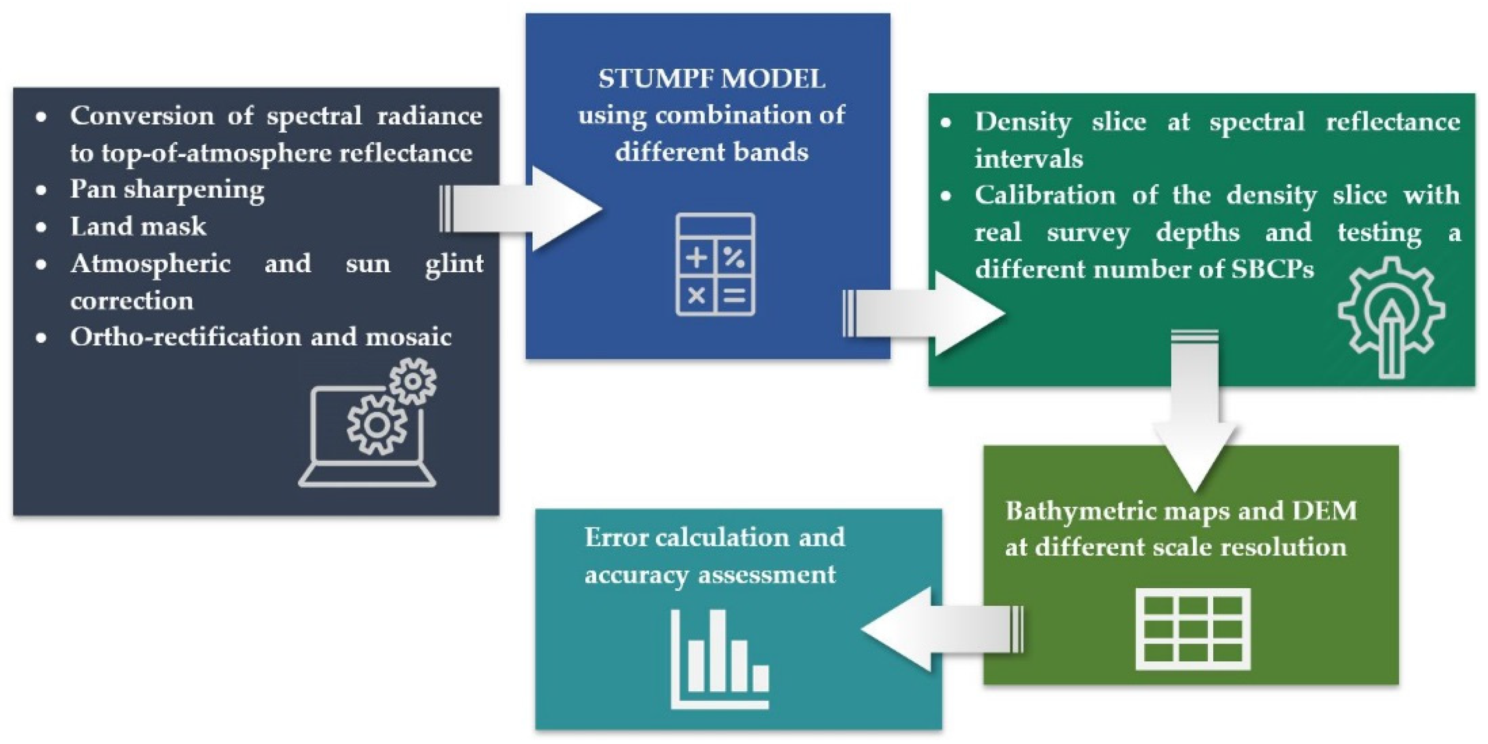
A set of Ground Control Points (GCPs), taken from the regional cartography, were used for the satellite image ortho-rectification and processed with the rational polynomial functions model. To preserve the original radiometric data, the nearest neighbor resampling method was adopted. Finally, thresholding on band 7 (near-infrared 1) was performed to mask out the land and the Stumpf SDB method was applied using 186 SBCPs distributed across the entire c.a. 4 km area and selected from the hydrographic survey dataset. The processing steps of generating bathymetric maps using SDB are illustrated in Figure 3.
2.4. UAV Multispectral Survey
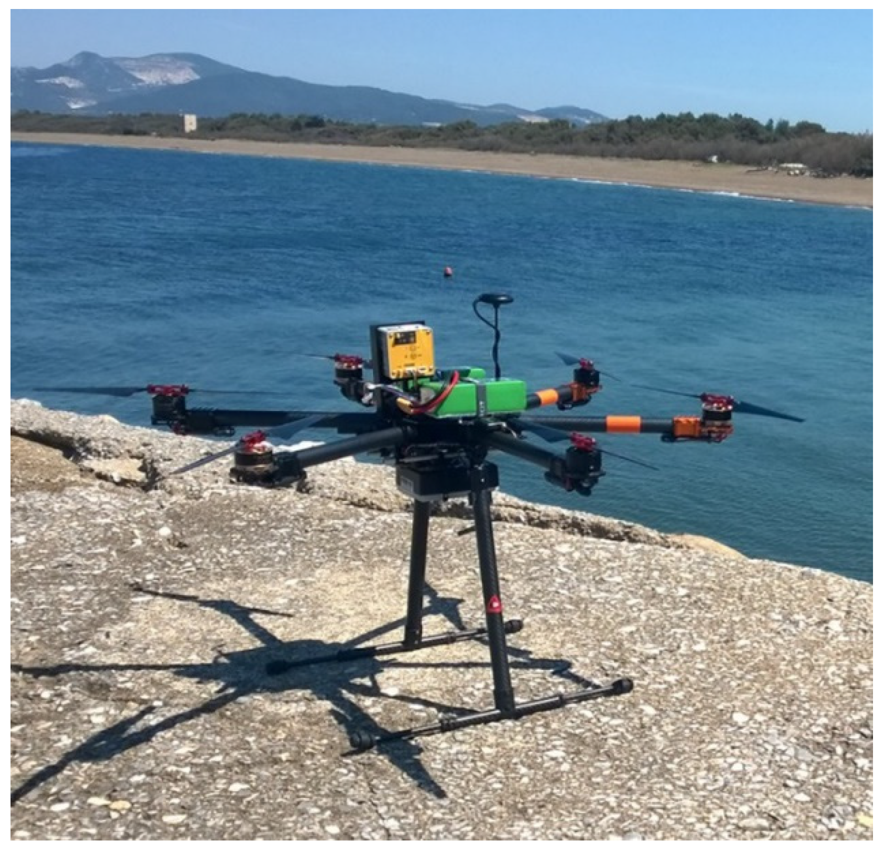
For the UAV survey, a HexaCopter drone equipped with a light multispectral camera, MAIA WV, and a log recording GPS for Post Processing Kinematic (PPK) data elaboration were used (Figure 4). The camera has an array of nine 1.2 Mpixel sensors (8 multispectral + 1 RGB) acquiring images in the VIS-NIR spectrum from 390 to 950 nm. The spectral bands have the same wavelength intervals of the WV2 satellite sensor—433–875 nm. In addition, an RGB color image is available live during capture. CMOS sensors settled in MAIA have 1280 × 960 pixels and the dimension of each pixel is 3.75 × 3.75 μm. The camera has an exposure interval of 0.1–50 ms, with a typical exposure time of 1 ms, and uses global shutter sensors. In this way, it is not necessary to stabilize it with gimbal, which is indispensable when using rolling shutter sensors, in order to avoid distortion, crawling, and blurring pixels in the images. In cameras that use a global shutter sensor, all the pixels that make up an image are captured at the same time. This means that the image will be “frozen”, minimalizing the blur effect. When using multispectral cameras with drones, this feature assumes great importance as the shots take place in motion.
MAIA’s proprietary image pre-processing software allows radial and geometrical distortion in the raw images to be corrected. It also allows every single band image to be combined into one multispectral file with pixel–pixel convergence.
The UAV flight was performed in April 2018 and 12 multispectral images were taken at a 150 m height, with about 10% overlap (Figure 5). The run was conducted in good weather on a non windy day in the early hours of the morning, in order to reduce the sun’s glint.
2.5. UAV Data Processing
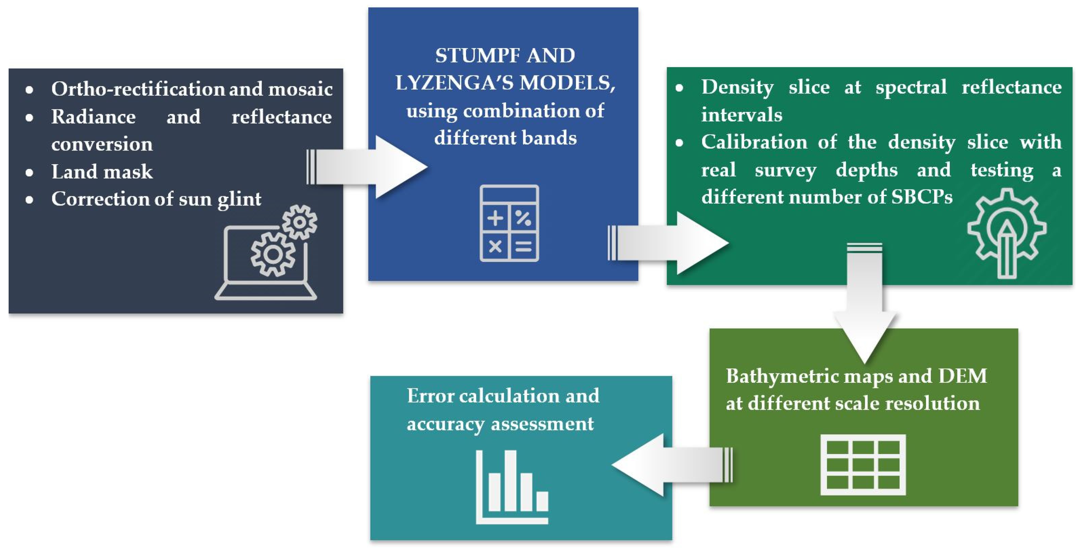
During a low altitude flight, as for a UAV, this sun effect produces a perturbation on the water surface that is difficult to correct. The data were elaborated using the Hedley method [71] to reduce this effect.
Because of the high percentage of water present in all the acquired images, a traditional Structure for Motion (SfM) technique and image bundle adjustment could not be used to produce the orthophoto. A different methodology had to be applied. The camera ground footprint was verified on the land using a GPS-RTK survey, and the size resulted in 96 × 72 m taken from a nadiral shot.
To address these issues, we developed an empirical solution georeferencing the images with a simple calculation programmed by the authors. By knowing the theoretical picture footprint sizes and their position from the internal PPK GPS and using heading and motion angle values recorded in the UAV control-unit flight, we could calculate their final planar deformation. The GPS processing was conducted with Leica LGO software using a Rinex file of the nearest GPS national network station. A final multispectral GeoTIFF image-mosaic was produced. The spatial accuracy was tested using two sea control points, represented by two buoys equipped with GPS that recorded the position in real-time. One of their instantaneous positions is shown in Figure 5 with red circles. The other three ground control points were located on the emerged beach near the shoreline. A maximum difference of 2.8 m between these points’ position and relative image pixel was found.
For this processing, empirical Satellite-Derived Bathymetry (SDB) methods were applied with UAV multispectral images, and were therefore renamed UDB.
For UAV bathymetry calibration, a different number of Sea Bottom Control Points (SBCPs) were tested (50, 200, and 500). These points were chosen so as to be uniformly distributed over the whole area with different grid cell values, according to the three SBCP datasets.
Figure 6 illustrates the steps of generating bathymetric maps using UDB.
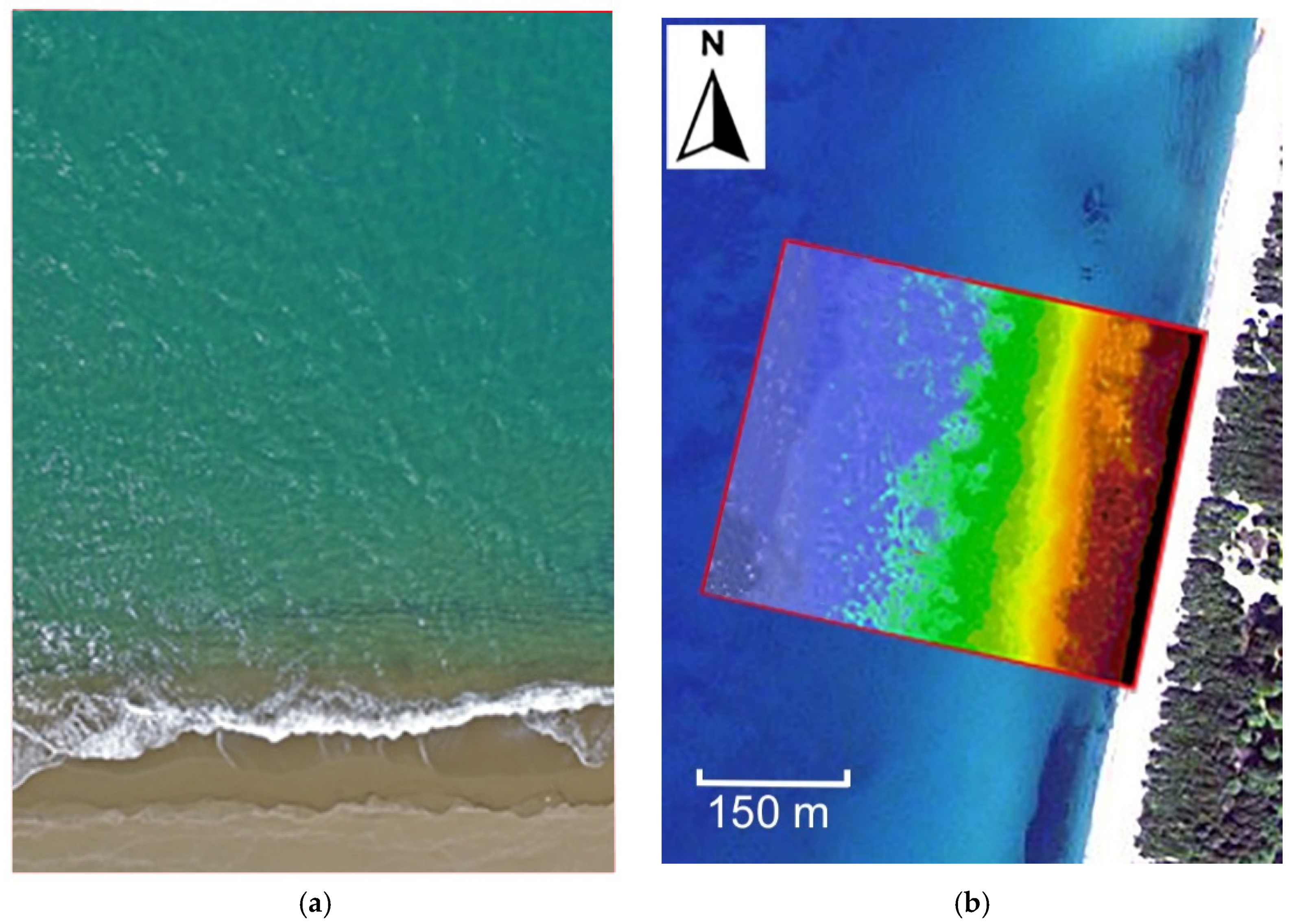
Figure 7 presents an example of one of the twelve RGB images acquired with the UAV multispectral camera (a) and the UDB map (b) inside the study area, performed by applying Stumpf’s model. At this point, the results were relative, since they did not represent absolute water depths. Instead, warm colors indicate shallow water and cold ones a greater depth, and the emerged beach is masked with a black color. The background image is the WV2.
2.6. In Situ Bathymetric Survey
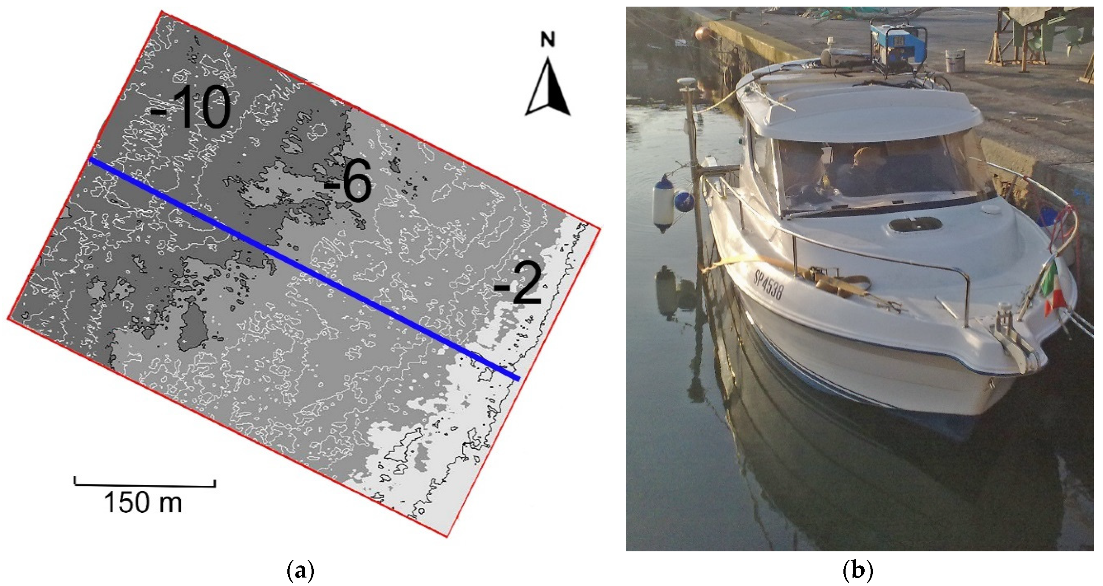
Four days of calm sea after the flight with the drone, a traditional hydrographic survey was conducted in the area using an SbEs for very shallow waters and an MbEs up to a −12 m depth (Figure 8a). For this work, a boat equipped with an R2Sonic 2022 multibeam mounted pole, Teledyne Mahrs motion sensor/gyro, GPS RTK, and Hypack2018 acquisition software was used (Figure 8b). The survey was carried out in the absence of wind and with calm seas and was conducted and calibrated according to IHO S-44 specifications [23], in order to guarantee the accuracy of the measurements. From this survey, a 3 × 3 m DEM of the sea bottom was finally produced. The same geodesy of the UAV survey was applied, and the measurements were also corrected for the low tide present in this area.
The survey shows that the main morphological variations in the area are located in the area limited by the shoreline and the surf zone down to a 4 m depth. From a 5 m depth, the bottom slope is more regular, with some irregularity due to the presence of Posidonia Oceanica meadow at the deeper edge. The bathymetric survey dataset was used for verification of the accuracy of the method and validation of the results.
3. Results
UAV- and satellite (SAT)-derived bathymetries from multispectral images were compared to the real bathymetry performed in the study area, where about 28,000 points were acquired during the hydrographic survey.
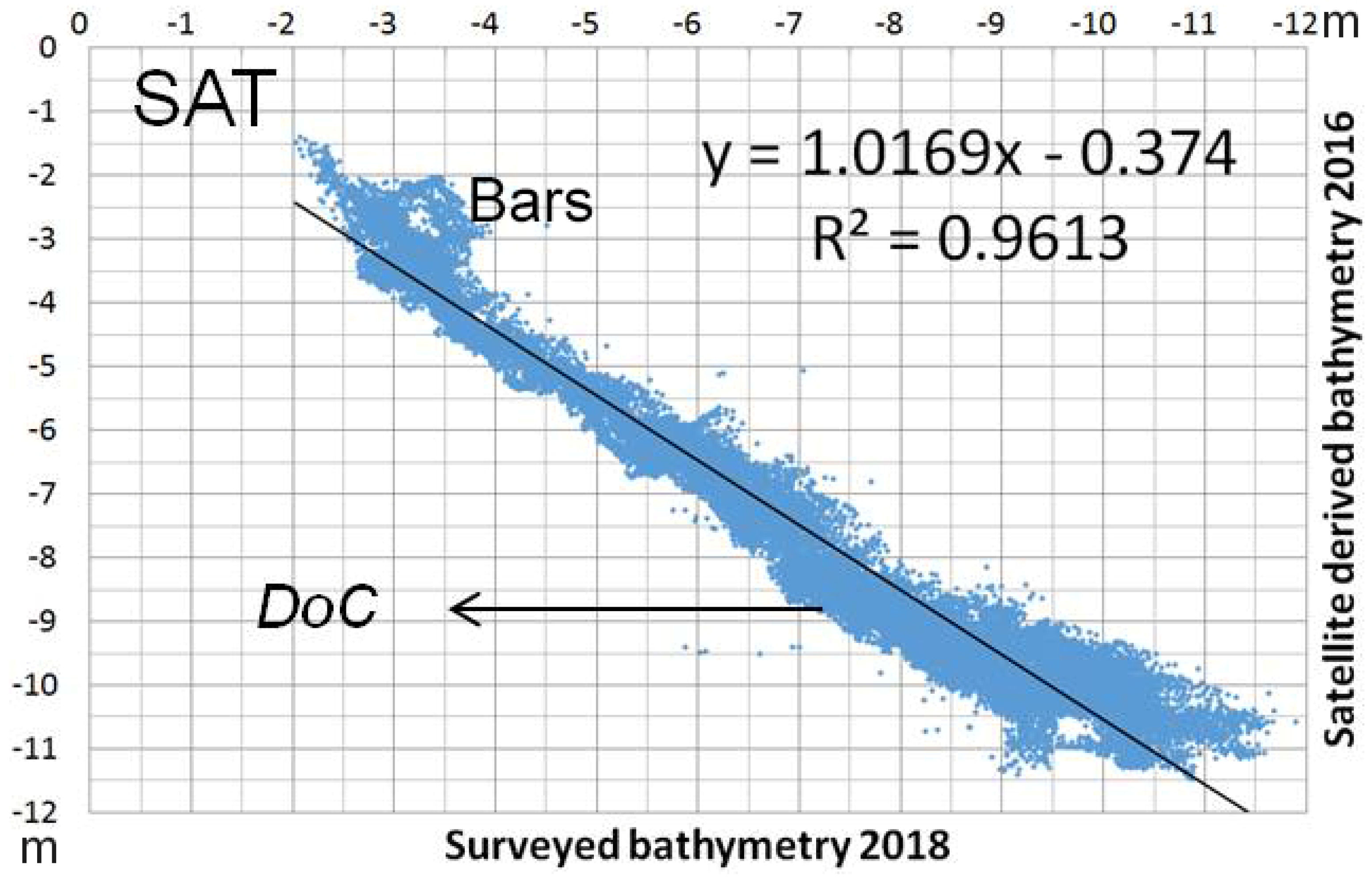
The research was initially conducted by comparing satellite- and UAV-derived bathymetries obtained from multispectral images, using the ratio log-transformation algorithm. Figure 9 shows a scatter plot of Satellite-Derived Bathymetry using the Stumpf algorithm and the real points dataset of the water depths. The plot shows a point dispersion higher in the surf zone and growing with the sea depth. In the deeper part of the profile, a poor correlation may be explained by the inaccuracy of the methodology because of the lower electromagnetic radiation efficiency; the dispersive data pattern in the nearshore area were caused by morphological variation due to the gap of time between the in situ survey and image acquisition. Unfortunately, it is not easy to find high-resolution satellite images with good overcast weather and sea conditions and this was closer in time to our hydrographic and UAV survey period. This fact can represent a serious impediment, especially when it is necessary to carry out investigations relating to a specific period, as in the case of much monitoring.
Satellite-Derived Bathymetry (SDB) fit the sea bottom between the surf zone and a c.a. −7 m depth better, while in the offshore and nearshore area it underestimated the real bathymetry. Overestimation was noticed between a −7 and −9 m depth, at approximately the depth of closure of sediment (DOC) in this area.
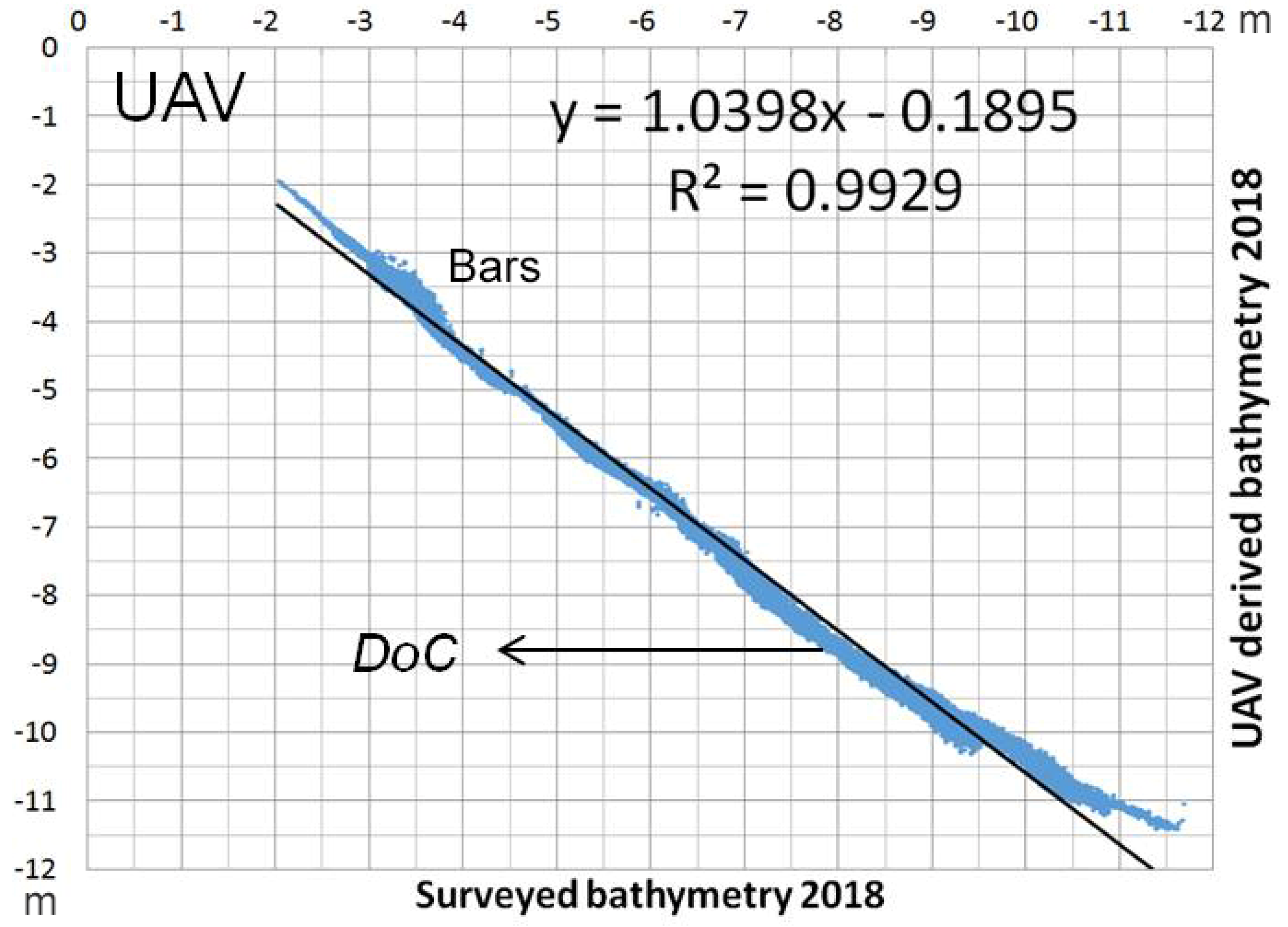
Figure 10 illustrates a scatter plot with UAV-Derived Bathymetry (UDB) and a real in-situ acoustic survey. The correlation is higher than in the previous plot, with a lower point dispersion. The higher coefficient of determination is an indicator of the better goodness of fit for the observations. This indicates a higher degree of confidence in the UDB results than SDB.
In very shallow and deep waters, the method underestimated the real bottom topography, as explained at the beginning of the Results paragraph. On the contrary, it is possible to notice a little overestimation in the central part of the profile, increasing down to a 10 m depth.
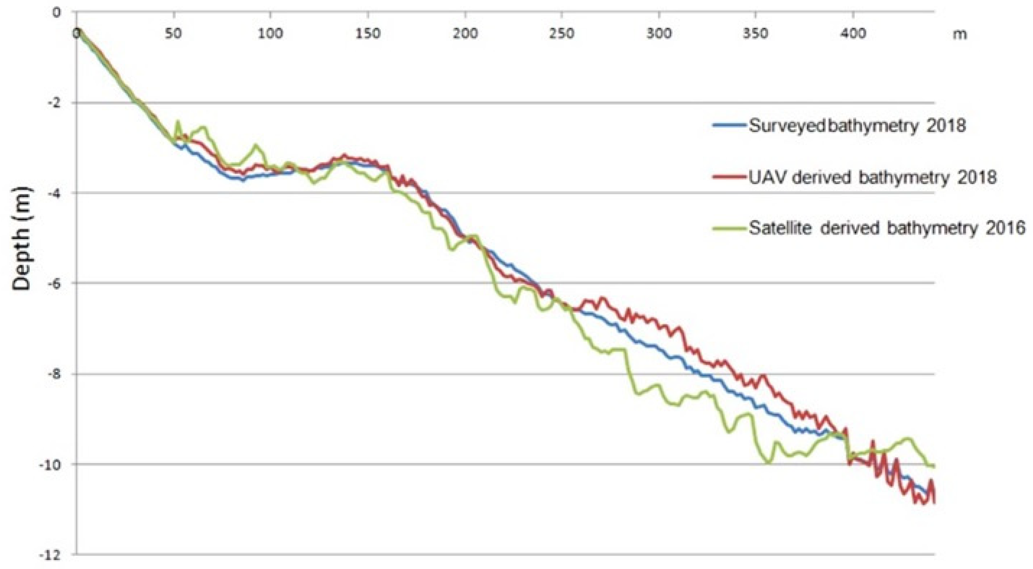
The results of the comparative analysis between the in situ survey and satellite (SAT) or UAV-Derived bathymetries produced with the Stumpf method are presented in Figure 11 for a beach profile located in the center of the study area (Figure 8a). A higher deviation of SDB than UDB from the real bottom is generally visible along with all the profiles. Both deviations also increase with the depth of the bottom.
Verification of the results was also conducted by considering the complete real bathymetric survey measurement dataset (28,000 points) and comparing it with satellite and UDB values (m).
The mean absolute deviation (MAD) was calculated to furnish the statistical dispersion or variability of the UAV bathymetry deviation from the surveyed data.
When analyzing the statistics of measured and estimated values, it must be considered that traditional echosounder bathymetric surveys are also affected by errors that can be evaluated in +/−10 cm [72]. The satellite and UAV images, using Stumpf’s algorithm, were also processed with optimal band ratio analysis (OBRA) methods. Our results show the best satellite and UAV band combination in the test area and conditions of blue (440–510 nm)/green (520–590 nm), with the best MAD of 0.21 cm for UDB down to a 5 m depth and 0.29 m using coastal-blue/green bands. Worse results were obtained using the UDB yellow/green and green/red ratios, with values of 0.31 and 0.35 cm, respectively. On the contrary, SDB exhibited higher results with real values. MAD results for different methodologies and band combinations at different depth ranges are shown in Table 1 and Table 2.
Data processing was also carried out to verify the minimum number of calibration points required to obtain the most accurate estimated bathymetry. Our research and verification indicate that, down to a 5 m depth, the difference in terms of the accuracy is less than 1% of the depth using 50, 200, or 500 points. We did not notice any appreciable variation in computing differences in elevation maps when changing the number of calibration points.
In a second phase, UAV-derived bathymetry using the Lyzenga algorithm was tested. Moreover, in this case, an assessment of the accuracy was conducted by comparing the UDB data, generated by this model, with the real bathymetry (full dataset) acquired by the traditional bathymetric survey with echosounders. The results were also compared to SDB using the Stumpf model.
Both methods show increasing point dispersion with the depth and in the surf zone at around a 4 m depth. The latter can be explained by the fact that the bathymetric survey was performed a few days after the UAV flight and the bars were in very dynamic area with calm seas. The increase in dispersion after the depth of closure of the sediments, with a value of around −9 m for this area, must be attributed to the decreasing of the accuracy with the depth of this methodology.
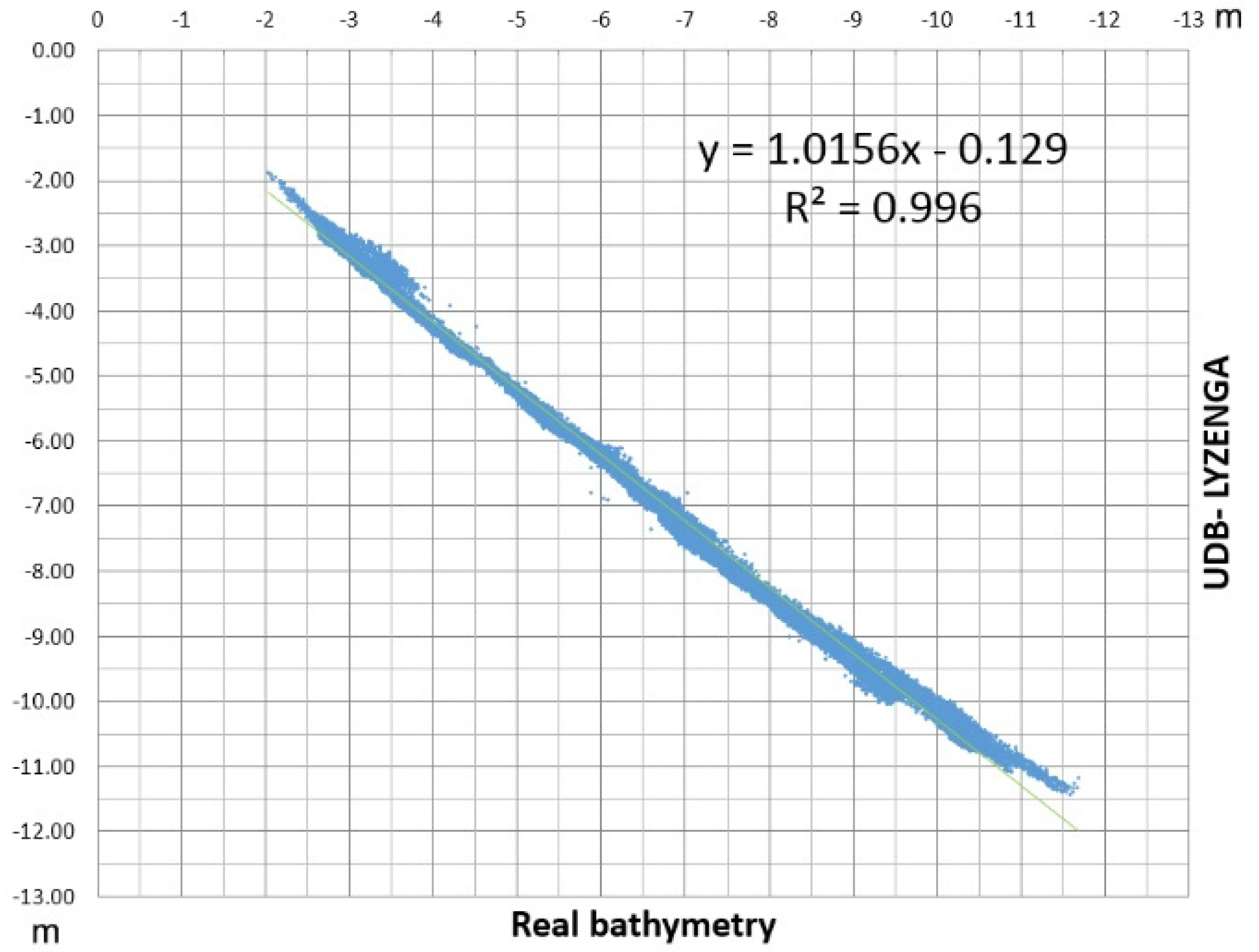
In the UDB (Lyzenga model) vs. surveyed bathymetry graph (Figure 12), it is shown that the spread of the data is lower than for the UDB (Stumpf model) method and the correlation is higher; a coefficient of determination of 0.996 indicates a better fitting of the data by the regression equation. Furthermore, in this case, underestimation is more evident in shallow and deep water, whereas, from a 5 to 10 m depth, overestimation occurs.
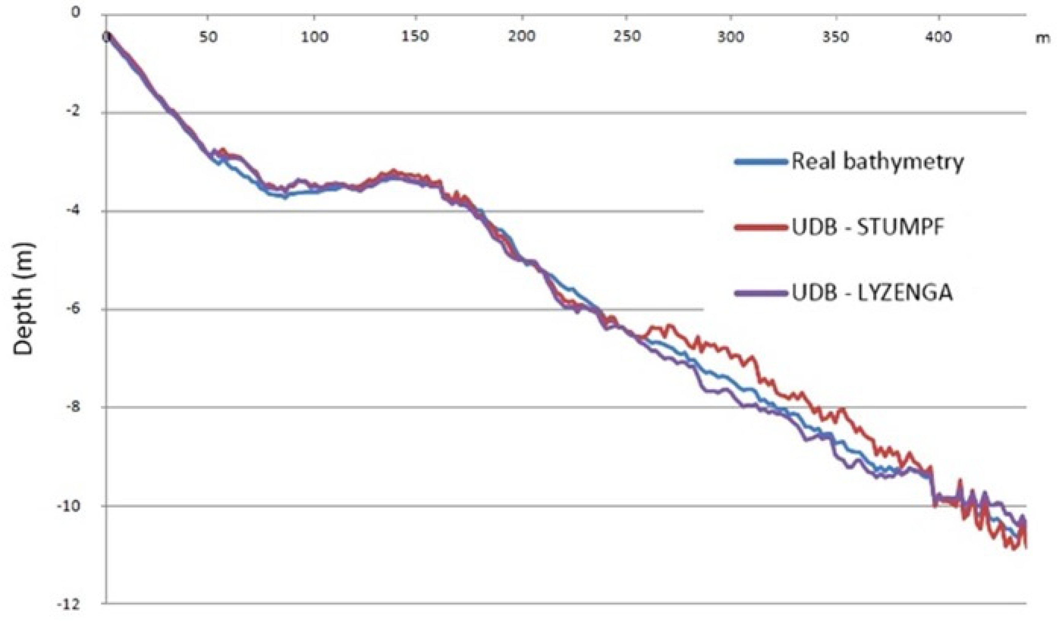
Figure 13 illustrates the comparison of real bathymetry and estimated values using Stumpf and Lyzenga algorithms for the same profile as in Figure 8. A larger deviation from measured data is evident, especially for deeper points.
Figure 14a presents a map of the study area, representing the change in altitude between the DEM of the sea bottom, obtained with the surveyed bathymetry, and the SDB using Stumpf’s model. In the same way, Figure 14b shows a map with UDB and Lyzenga’s model. It is graphically evident that, in the map on the right (b), the differences with the real sea bottom topography are smaller and of the order of a few decimeters, especially in shallow waters. The plots show the difference (derived minus survey) between the two estimates.
Verification of the UAV-derived bathymetry results was also conducted by considering the complete in situ survey dataset and comparing it with Lyzenga-UDB values (m). The final MAD results of different depth ranges are shown in Table 3.
To assess the accuracy and the precision of the UDB measurement systems, the Root Mean Squared Error (RMSE) was also calculated for both the Lyzenga and Stumpf method (Table 4).
4. Discussion
In this study, Stumpf and Lyzenga models have been applied to derive the bathymetry using an UAV equipped with a multispectral camera. In general, both models produced encouraging results. Stumpf processing is simpler compared to Lyzenga processing, which requires multiple regression methods, but delivers slightly rough results.
The preliminary results show that the use of a professional multispectral sensor, mounted on a UAV platform, permits a higher degree of accuracy and efficiency to be achieved in the bathymetric survey, not only compared to satellite-derived bathymetry, but also to the global literature research and methods based on the use of drones equipped with other different remote, active, and passive sensors.
As for providing ready-to-use data, using UAVs is an immediate method to be applied, which helps any time such data are necessary for field activities for which the execution is required immediately after the completion of the survey (e.g., sediment or water sampling) or in cases of urgent coastal monitoring necessities. It must also be considered that the use of UAV can be coupled, using a high-resolution RGB camera, with a 3D SfM survey of the emerged coastlines and can be considered the most effective and cost-efficient technology for capturing both the land and seafloor simultaneously, in order to provide a continuous, detailed 3D elevation model of the surveyed area. On the contrary, UAV acquisition data are applicable to areas with kilometrical development, while the satellite images can be used to derive the bathymetry of extended areas. Drone surveys are restricted to relatively small areas due to the battery limitations of quadcopters and fixed wing unmanned aerial vehicles. Similar to the SDB, this method cannot be used in the presence of increased turbidity or larger breaking waves and calibration points are always required. The advantage is that a UAV survey can be easily rescheduled to a day with better water conditions.
The most difficult processing and that which could be improved concerns the orthorectification of images, given the fact that, in order to produce the final orthophoto, a bundle adjustment of the images cannot be used due to the presence of too much water, the depth of the survey down to about −11 m and the sandy bottom of beach. The method here proposed could be improved; however, being enough for the purpose of this kind of application also with a 5 × 5 m cell grid DTM, flights at higher altitudes could be performed when permitted or through special permits, in order to reduce the number of the images and have less optical distortion. Moreover, the buoys, or alternative targets equipped with GPS, could also be used to directly perform the single image orthorectification, using their position as control points, but they should be moved following the drone track.
5. Conclusions
Principally, this paper has successfully illuminated the level of quality that the UAV-derived bathymetry (UDB) technology can offer to the hydrographic surveying industry and demonstrated that this methodology can be used to extract bathymetric data in small areas with better accuracy than that of established by satellite-derived bathymetry (SDB) methods. The first objective of this research was to explore the potential of UDB using Stumpf and Lyzenga models, which are two of the most common and cited algorithms in the scientific literature and have previously been applied for satellite multispectral image processing. The models used by Stumpf and Lyzenga may prove worthy of adoption for the regular monitoring of sensitive coastal areas, as their algorithms yielded accurate results in the study area when estimating the depth of shallow waters and homogeneous seabed. The results show how Lyzenga’s accuracy seems to be slightly higher than that of Stumpf’s model in our research conditions.
UDB results are more accurate than those of satellite-derived bathymetry because of the higher image details. The use of satellite imaging for sea bottom monitoring is in fact prone to shortcomings in terms of data acquisition in the presence of overcast weather and/or adverse sea conditions. On the other hand, UDB does not require any atmospheric correction procedure, and in small to medium size areas, it allows an easier and cheaper acquisition of images for coastal monitoring. Our results also confirm the literature results in terms of satellite-derived bathymetry’s accuracy. Due to the length of time that elapses between the collection of satellite images and the ground truth bathymetric survey, not only are the surveys conducted a significant time apart, but probabilistically, the beach and nearshore are likely to be in two different states, given the seasonality in wave climate. For this reason, it is difficult to draw a comparison and conclusion on the accuracy of the methods based on these two datasets.
Finally, UDB provides a detection accuracy of about 20 cm (down to a 5 m depth) and allows the dry beach topography to be connected to the MbEs survey at a depth (0–2 m) inaccessible or too time-consuming for a hydrographic survey with this kind of echosounder equipment.
In this condition, UAV technology can also be used as an alternative to MbEs surveys, where the centimetric precision is not required. It is really important to think about the objectives that need to be reached using remote sensing and fully explore alternatives in terms of costs and effectiveness, and we must remember that some objectives will not be achievable using these technologies.
In the face of its many upsides, the use of UAV as a tool for shallow water bathymetry requires further testing, which will lead to a better understanding of the limits and potential of this method and therefore to the design of a reliable standardized data acquisition process. It will be necessary to test, where possible, flights at higher altitudes to optimize the image orthorectification and coastal sites with different characteristics, in order to analyze the confidence intervals for the coefficient of variation as a function of the water turbidity and surface condition and the seabed’s nature or morphology.
Author Contributions
Conceptualization, L.R.; methodology, L.R., I.M., and F.P.; writing—original draft preparation, L.R., I.M., and F.P.; writing—review and editing, L.R., I.M., and F.P. All authors have read and agreed to the published version of the manuscript.
Funding
This research received no external funding.
Conflicts of Interest
The authors declare no conflict of interest.
References
- Neeman, N.; Servis, J.A.; Naro-Maciel, E. Conservation Issues: Oceanic Ecosystems. In Reference Module in Earth Systems and Environmental Sciences; Elsevier: Amsterdam, The Netherlands, 2015. [Google Scholar]
- Bush, D.M.; Pilkey, O.H.; Neal, W.J. Human impact on coastal topography. Encycl. Ocean Sci. 2001, 1, 480–489. [Google Scholar]
- Labuz, T.A. Environmental Impacts—Coastal Erosion and Coastline Changes. In Second Assessment of Climate Change for the Baltic Sea Basin; The BACC II Author Team, Ed.; Regional Climate Studies; Springer: Cham, Switzerland, 2015. [Google Scholar]
- Dronkers, J. Dynamics of Coastal Systems; Advanced Series on Ocean Engineering; World Scientific Publishing Ltd.: Singapore; Hackensack, NJ, USA, 2005. [Google Scholar]
- Neumann, B.; Vafeidis, A.T.; Zimmermann, J.; Nicholls, R.J. Future Coastal Population Growth and Exposure to Sea-Level Rise and Coastal Flooding—A Global Assessment. PLoS ONE 2015, 10, e0118571. [Google Scholar] [CrossRef] [PubMed] [Green Version]
- Gilbert, J.; Vellinga, P. Coastal Zone Management in Climate Change: The IPCC Response Strategies. 2005, pp. 133–159. Available online: https://www.ipcc.ch/site/assets/uploads/2018/03/ipcc_far_wg_III_full_report.pdf (accessed on 25 November 2020).
- Day, J. The need and practice of monitoring, evaluating and adapting marine planning and management. Mar. Policy 2008, 32, 823–831. [Google Scholar] [CrossRef]
- Douvere, F.; Ehler, C.N. The importance of monitoring and evaluation in adaptive maritime spatial planning. J. Coast. Conserv. 2010, 15, 305–311. [Google Scholar] [CrossRef]
- Bio, A.; Bastos, L.; Granja, H.; Pinho, J.L.S.; Goncalves, J.A.; Henriques, R.; Madeira, S.; Magalhàes, A.; Rodrigues, D. Methods for coastal monitoring and erosion risk assessment: Two Portuguese case studies. J. Integr. Coast. Zone Manag. 2015, 15, 47–63. [Google Scholar] [CrossRef] [Green Version]
- Mentaschi, L.; Vousdoukas, M.I.; Pekel, J.-F.; Voukouvalas, E.; Feyen, L. Global long-term observations of coastal erosion and accretion. Sci. Rep. 2018, 8, 12876. [Google Scholar] [CrossRef] [PubMed] [Green Version]
- Prasetya, G. Protection from Coastal Erosion; Food and Agriculture Organisation: Rome, Italy, 2007. [Google Scholar]
- Klemas, V.V. Coastal and Environmental Remote Sensing from Unmanned Aerial Vehicles: An Overview. J. Coast. Res. 2015, 315, 1260–1267. [Google Scholar] [CrossRef] [Green Version]
- Pe’eri, S.; Long, B. LIDAR Technology Applied in Coastal Studies and Management. J. Coast. Res. 2011, 62, 1–5. [Google Scholar] [CrossRef]
- Westoby, M.J.; Brasington, J.; Glasser, N.F.; Hambrey, M.J.; Reynolds, J.M. “Structure-from-Motion” photogrammetry: A low-cost, effective tool for geoscience applications. Geomorphology 2012, 179, 300–314. [Google Scholar] [CrossRef] [Green Version]
- Papakonstantinou, A.; Topouzelis, K.; Pavlogeorgatos, G. Coastline Zones Identification and 3D Coastal Mapping Using UAV Spatial Data. ISPRS Int. J. Geo-Inf. 2016, 5, 75. [Google Scholar] [CrossRef] [Green Version]
- Casella, E.; Drechsel, J.; Winter, C.; Benninghoff, M.; Rovere, A. Accuracy of sand beach topography surveying by drones and photogrammetry. Geo-Mar. Lett. 2020, 40, 255–268. [Google Scholar] [CrossRef] [Green Version]
- Laporte-Fauret, Q.; Marieu, V.; Castelle, B.; Michalet, R.; Bujan, S.; Rosebery, D. Low-Cost UAV for High-Resolution and Large-Scale Coastal Dune Change Monitoring Using Photogrammetry. J. Mar. Sci. Eng. 2019, 7, 63. [Google Scholar] [CrossRef] [Green Version]
- Zhou, G.; Ming, X. Coastal 3-D Morphological Change Analysis Using LiDAR Series Data: A Case Study of Assateague Island National Seashore. J. Coast. Res. 2009, 252, 435–447. [Google Scholar] [CrossRef]
- Nasu, N.; Honjo, S. New Directions of Oceanographic Research and Development; Springer: Tokyo, Japan, 1993. [Google Scholar]
- Fumagalli, E.; Bibuli, M.; Caccia, M.; Zereik, E.; Fabrizio Del, B.; Gasperini, L.; Giuseppe, S.; Bruzzone, G. Combined Acoustic and Video Characterization of Coastal Environment by means of Unmanned Surface Vehicles. In Proceedings of the 19th World Congress, The International Federation of Automatic Control, Cape Town, South Africa, 24–29 August 2014; pp. 24–29. [Google Scholar]
- Muzirafuti, A.; Barreca, G.; Crupi, A.; Faina, G.; Paltrinieri, D.; Lanza, S.; Randazzo, G. The Contribution of Multispectral Satellite Image to Shallow Water Bathymetry Mapping on the Coast of Misano Adriatico, Italy. J. Mar. Sci. Eng. 2020, 8, 126. [Google Scholar] [CrossRef] [Green Version]
- Federation Iinternationale des Geometres FIG. Guidelines for the Planning, Execution and Management of Hydrographic Surveys in Ports and Harbours. Int. Fed. Surv. FIG Comm. 2010, 4, 56. [Google Scholar]
- International Hydrographic Organization (IHO). IHO Standards for Hydrographic Surveys, 5th ed.; International Hydrographic Bureau: Monte Carlo, Monaco, 2018. [Google Scholar]
- Pranzini, E.; Rossi, L. The role of coastal erosion monitoring. In Coastal Erosion Monitoring; Cipriani, L.E., Ed.; Nuova Grafica Fiorentina: Firenze, Italy, 2013; pp. 11–55. [Google Scholar]
- Gasperini, L. Extremely Shallow-water Morphobathymetric Surveys: The Valle Fattibello (Comacchio, Italy) Test Case. Mar. Geophys. Res. 2005, 26, 97–107. [Google Scholar] [CrossRef]
- Giordano, F.; Mattei, G.; Parente, C.; Peluso, F.; Santamaria, R. Integrating Sensors into a Marine Drone for Bathymetric 3D Surveys in Shallow Waters. Sensors 2015, 16, 41. [Google Scholar] [CrossRef] [Green Version]
- Wang, C.K.; Philpot, W.D. Using Airborne Bathymetric Lidar to Detect Bottom Type Variation in Shallow Waters. Remote Sens. Environ. 2017, 106, 123–135. [Google Scholar] [CrossRef]
- Jégat, V.; Pe’eri, S.; Freire, R.; Klemn, A.; Nyberg, J. Satellite-Derived Bathymetry: Performance and Production. In Proceedings of the Canadian Hydrographic Conference, Halifax, NS, Canada, 16–19 May 2016. [Google Scholar]
- Doxani, G.; Papadopoulou, M.; Lafazani, P.; Pikridas, C.; Tsakiri-Strati, M. Shallow-water bathymetry over variable bottom types using multispectral worldview-2 image. Int. Arch. Photogramm. Remote Sens. Spat. Inf. Sci. 2012, 39, 159–164. [Google Scholar] [CrossRef] [Green Version]
- Jawak, S.D.; Vadlamani, S.S.; Luis, A.J. A Synoptic Review on Deriving Bathymetry Information Using Remote Sensing Technologies: Models, Methods and Comparisons. Adv. Remote Sens. 2015, 4, 147–162. [Google Scholar] [CrossRef] [Green Version]
- Deng, Z.; Ji, M.; Zhang, Z. Mapping bathymetry from multi-source remote sensing images: A case study in the Beilun Estuary, Guangxi, China. Int. Arch. Photogramm. Remote Sens. Spat. Inf. Sci. 2008, 37, 1321–1326. [Google Scholar]
- Said, M.; Mahmud, M.; Hasan, M. Satellite-derived bathymetry: Accuracy assessment on depths derivation algorithm for shallow water area. Int. Arch. Photogramm. Remote Sens. Spat. Inf. Sci. 2017, XLII-4/W5, 159–164. [Google Scholar] [CrossRef] [Green Version]
- Traganos, D.; Poursanidis, D.; Aggarwal, B.; Chrysoulakis, N.; Reinartz, P. Estimating Satellite-Derived Bathymetry (SDB) with the Google Earth Engine and Sentinel-2. Remote Sens. 2018, 10, 859. [Google Scholar] [CrossRef] [Green Version]
- Caballero, I.; Stumpf, R.P. Towards Routine Mapping of Shallow Bathymetry in Environments with Variable Turbidity: Contribution of Sentinel-2A/B Satellites Mission. Remote Sens. 2020, 12, 451. [Google Scholar] [CrossRef] [Green Version]
- Hamylton, S.M.; Hedley, J.D.; Beaman, R.J. Derivation of High-Resolution Bathymetry from Multispectral Satellite Imagery: A Comparison of Empirical and Optimisation Methods through Geographical Error Analysis. Remote Sens. 2015, 7, 16257–16273. [Google Scholar] [CrossRef] [Green Version]
- Philpott, W. Bathymetric mapping with passive multispectral imagery. Appl. Opt. 1989, 28, 1569–1578. [Google Scholar] [CrossRef] [PubMed]
- Gao, B.-C.; Montes, M.J.; Li, R.-R.; Dierssen, H.M.; Davis, C.O. An Atmospheric Correction Algorithm for Remote Sensing of Bright Coastal Waters Using MODIS Land and Ocean Channels in the Solar Spectral Region. IEEE Trans. Geosci. Remote Sens. 2007, 45, 1835–1843. [Google Scholar] [CrossRef]
- Joshi, I.D.; DSa, E.J.; Osburn, C.L.; Bianchi, T.S. Turbidity in Apalachicola Bay, Florida from Landsat 5 TM and Field Data: Seasonal Patterns and Response to Extreme Events. Remote Sens. 2017, 9, 367. [Google Scholar] [CrossRef] [Green Version]
- Lyzenga, D.R. Passive remote sensing techniques for mapping water depth and bottom features. Appl. Opt. 1978, 17, 379–383. [Google Scholar] [CrossRef]
- Lyzenga, D.R. Remote sensing of bottom reflectance and water attenuation parameters in shallow water using Aircraft and Landsat data. Int. J. Remote Sens. 1981, 2, 72–82. [Google Scholar] [CrossRef]
- Lyzenga, D.R.; Malinas, N.; Tanis, F. Multispectral bathymetry using a simple physically based algorithm. IEEE Trans. Geosci. Remote Sens. 2006, 44, 2251–2259. [Google Scholar] [CrossRef]
- Jupp, D.L.B. Background and extensions to depth of penetration (DOP) mapping in shallow coastal waters. In Proceedings of the Symposium on Remote Sensing of the Coastal Zone, Gold Coast, Australia, 7–9 September 1988; Volume IV-2. [Google Scholar]
- Stumpf, R.P.; Holderied, K.; Sinclair, M. Determination of water depth with high-resolution satellite imagery over variable bottom types. Limnol. Oceanogr. 2003, 48, 547–556. [Google Scholar] [CrossRef]
- Panchang, V.; Kaihatu, J.M. Advances in Coastal Hydraulics; World Scientific Publishing Ltd.: Singapore; Hackensack, NJ, USA, 2018. [Google Scholar]
- Flener, C.; Lotsari, E.; Alho, P.; Kayhko, J. Comparison of Empirical and Theoretical Remote Sensing Based Bathymetry Models in River Environments. River Res. Appl. 2012, 28, 118–133. [Google Scholar] [CrossRef]
- Toro, G.F.; Tsourdos, A. UAV or Drones for Remote Sensing Applications; MDPI: Basel, Switzerland, 2018; Volume 2. [Google Scholar]
- Gonçalves, J.A.; Henriques, R. UAV photogrammetry for topographic monitoring of coastal areas. ISPRS J. Photogramm. Remote Sens. 2015, 104, 101–111. [Google Scholar] [CrossRef]
- Long, N.; Millescamps, B.; Pouget, F.; Dumon, A.; Lachaussée, N.; Bertin, X. Accuracy assessment of coastal topography derived from UAV images. Int. Arch. Photogramm. Remote Sens. Spat. Inf. Sci. 2016, XLI-B1, 1127–1134. [Google Scholar] [CrossRef]
- Taddia, Y.; Russo, P.; Lovo, S.; Pellegrinelli, A. Multispectral UAV monitoring of submerged seaweed in shallow water. Appl. Geomat. 2020, 12, 19–34. [Google Scholar] [CrossRef] [Green Version]
- Remondino, F.; Barazzetti, L.; Nex, F.; Scaioni, M.; Sarazzi, D. UAV Photogrammetry for mapping and 3D modeling–Current status and future perspectives. Int. Arch. Photogramm. Remote. Sens. Spat. Inf. Sci. 2011, XXXVIII-1/C22, 25–31. [Google Scholar] [CrossRef] [Green Version]
- Jeziorska, J. UAS for Wetland Mapping and Hydrological Modeling. Remote Sens. 2019, 11, 1997. [Google Scholar] [CrossRef] [Green Version]
- Nex, F.; Remondino, F. UAV for 3D mapping applications: A review. Appl. Geomat. 2013, 6, 1–15. [Google Scholar] [CrossRef]
- Turner, I.L.; Harley, M.D.; Drummond, C.D. UAVs for coastal surveying. Coast. Eng. 2016, 114, 19–24. [Google Scholar] [CrossRef]
- Mandlburger, G.; Pfennigbauer, M.; Wieser, M.; Riegl, U.; Pfeifer, N. Evaluation of a Novel UAV-BORNE Topo-Bathymetric Laser Profiler. Int. Arch. Photogramm. Remote Sens. Spat. Inf. Sci. 2016, XLI-B1, 933–939. [Google Scholar] [CrossRef]
- Bandini, F. Hydraulics and Drones: Observations of Water Level, Bathymetry and Water Surface Velocity from Unmanned Aerial Vehicles; Department of Environmental Engineering, Technical University of Denmark (DTU): Lyngby, Denmark, 2017. [Google Scholar]
- Jonathan, L.; Carrivick, M.; Smith, W. Fluvial and aquatic applications of Structure from Motion photogrammetry and unmanned aerial vehicle/drone technology. Wiley Interdiscip. Rev. Water 2019, 6, e1328. [Google Scholar]
- Casella, E.; Collin, A.; Harris, D.; Ferse, S.; Bejarano, S.; Parravicini, V.; Hench, J.L.; Rovere, A. Mapping coral reefs using consumer-grade drones and structure from motion photogrammetry techniques. Coral Reefs 2017, 36, 269–275. [Google Scholar] [CrossRef]
- Tamminga, A.; Hugenholtz, C.; Eaton, B.; Lapointe, M. Hyperspatial Remote Sensing of Channel Reach Morphology and Hydraulic Fish Habitat Using an Unmanned Aerial Vehicle (UAV): A first assessment in the Context of River Research and Management. River Res. Appl. 2015, 31, 379–391. [Google Scholar] [CrossRef]
- Fallati, L.; Saponari, L.; Savini, A.; Marchese, F.; Corselli, C.; Galli, P. Multi-Temporal UAV Data and Object-Based Image Analysis (OBIA) for Estimation of Substrate Changes in a Post-Bleaching Scenario on a Maldivian Reef. Remote. Sens. 2020, 12, 2093. [Google Scholar] [CrossRef]
- Ahn, K.; Oh, C.Y.; Park, Y.S.; Park, S.W. Passive Remote Sensing Using Drone and HD Camera for Mapping Surf Zone Bathymetry. In International Conference on Asian and Pacific Coasts, Proceedings of the APAC 2019, Hanoi, Vietnam, 25–28 September 2019; Trung Viet, N., Xiping, D., Thanh Tung, T., Eds.; Springer: Singapore, 2019. [Google Scholar]
- Agrafiotis, P.; Skarlatos, D.; Georgopoulos, A.; Karantzalos, K. Shallow Water Bathymetry Mapping from Uav Imagery Based on Machine Learning. ISPRS Int. Arch. Photogramm. Remote Sens. Spat. Inf. Sci 2019, XLII-2/W10, 9–16. [Google Scholar] [CrossRef] [Green Version]
- Plant, N.; Holman, R.; Holland, K.T. cBathy: A robust algorithm for estimating nearshore bathymetry. J. Geophys. Res. Oceans 2013, 118, 2595–2609. [Google Scholar]
- Matsuba, Y.; Sato, S. Nearshore bathymetry estimation using UAV. Coast. Eng. J. 2018, 60, 51–59. [Google Scholar] [CrossRef]
- Chirayath, V.; Earle, S.A. Drones that see through waves—Preliminary results from airborne fluid lensing for centimetre-scale aquatic conservation. Aquat. Conserv. Mar. Freshw. Ecosyst. 2013, 26 (Suppl. S2), 237–250. [Google Scholar] [CrossRef] [Green Version]
- Flener, C.; Vaaja, M.; Jaakkola, A.; Krooks, A.; Kaartinen, H.; Kukko, A.; Kasvi, E.; Hyyppä, H.; Hyyppä, J.; Alho, P. Seamless mapping of river channels at high resolution using mobile liDAR and UAV-photography. Remote Sens. 2013, 5, 6382–6407. [Google Scholar] [CrossRef] [Green Version]
- Zinke, P.; Flener, C. Experiences from the use of Unmanned Aerial Vehicles (UAV) for River Bathymetry Modelling in Norway. Vann 2013, 48, 351–360. [Google Scholar]
- Gentile, V.; Mrόz, M.; Spitoni, M.; Lejot, J.; Piégay, H.; Demarchi, L. Bathymetric Mapping of Shallow Rivers with UAV Hyperspectral Data. In Proceedings of the 5th International Conference on Telecommunications and Remote Sensing, Milan, Italy, 10–11 October 2016; pp. 43–49. [Google Scholar]
- Nebiker, S.; Lack, N.; Abächerli, M.; Läderach, S. Light-Weight multispectral UAV sensors and their capabilities for predicting grain yield and detecting plant diseases. Int. Arch. Photogramm. Remote Sens. Spat. Inf. Sci. 2016, XLI-B1, 12–19. [Google Scholar] [CrossRef]
- Rossi, L.; Mammì, I.; Pranzini, E. A comparison between UAV and high-resolution multispectral satellite images for bathymetry estimation. In Proceedings of the IX Conference of the Italian Society of Remote Sensing. Trends in Earth Observation: Earth Observation Advancements in a Changing World, Firenze, Italy, 30 November–1 December 2018; Volume 1, pp. 143–146. [Google Scholar]
- Pushparaj, J.; Hegde, A.V. Estimation of bathymetry along the coast of Mangaluru using Landsat-8 imagery. J. Ocean Clim. Sci. Technol. Impacts 2018, 8, 71–83. [Google Scholar] [CrossRef] [Green Version]
- Hedley, J.D.; Harborne, A.R.; Mumby, P.J. Simple and robust removal of sun glint for mapping shallow-water benthos. Int. J. Remote Sens. 2005, 26, 2107–2112. [Google Scholar] [CrossRef]
- Gibeaut, J.C.; Gutierrez, R.; Kyser, J.A. Increasing the Accuracy and Resolution of Coastal Bathymetric Surveys. J. Coast. Res. 1998, 14, 1082–1098. [Google Scholar]
Figure 1.
Location map, with the study area being located in the red rectangle.

Figure 2.
Satellite-Derived Bathymetry (SDB) and the WorldView-2 (WV2) RGB image showing the study area position.
Figure 2.
Satellite-Derived Bathymetry (SDB) and the WorldView-2 (WV2) RGB image showing the study area position.

Figure 3.
Satellite-Derived Bathymetry (SDB) image processing sequence.

Figure 4.
The Unmanned Aerial Vehicle (UAV) used for the survey, equipped with a MAIA multispectral camera.
Figure 4.
The Unmanned Aerial Vehicle (UAV) used for the survey, equipped with a MAIA multispectral camera.

Figure 5.
UAV flight plan in the study area, with the position of the two buoys and three Ground Control Points (GCPs) on the beach marked by red circles.
Figure 5.
UAV flight plan in the study area, with the position of the two buoys and three Ground Control Points (GCPs) on the beach marked by red circles.

Figure 6.
UAV-Derived Bathymetry (UDB) image processing sequence.

Figure 7.
Example of one of twelve UAV RGB images of 96 × 72 m (a) and a UDB relative water depth map in the study area acquired using the Stumpf method (b).
Figure 7.
Example of one of twelve UAV RGB images of 96 × 72 m (a) and a UDB relative water depth map in the study area acquired using the Stumpf method (b).

Figure 8.
(a) 2018 real bathymetric survey map of the study area and the position of a central profile in blue. Depth is expressed in meters. (b) The boat used for the survey, with the Multibeam Echosounder (MbEs) mounted on the pole with the GPS.
Figure 8.
(a) 2018 real bathymetric survey map of the study area and the position of a central profile in blue. Depth is expressed in meters. (b) The boat used for the survey, with the Multibeam Echosounder (MbEs) mounted on the pole with the GPS.

Figure 9.
SDB with Stumpf’s model and real bathymetry plot.

Figure 10.
UDB with Stumpf’s model and real bathymetry plot.

Figure 11.
SDB and UDB (Stumpf’s model) compared to a real surveyed profile, perpendicular to the shoreline and located in the center of the study area.
Figure 11.
SDB and UDB (Stumpf’s model) compared to a real surveyed profile, perpendicular to the shoreline and located in the center of the study area.

Figure 12.
UDB with Lyzenga model and real bathymetry plot.

Figure 13.
UDB with Lyzenga and Stumpf models and a real surveyed profile located in the center of the study area and perpendicular to the shoreline, as in Figure 4.
Figure 13.
UDB with Lyzenga and Stumpf models and a real surveyed profile located in the center of the study area and perpendicular to the shoreline, as in Figure 4.

Figure 14.
Differences in elevation maps using satellite-Stumpf- (a) and UAV-Lyzenga-derived (b) bathymetries and real survey in the study area.
Figure 14.
Differences in elevation maps using satellite-Stumpf- (a) and UAV-Lyzenga-derived (b) bathymetries and real survey in the study area.


Table 1.
The mean absolute deviation (MAD) (m) of different depth ranges and band combinations for UDB with Stumpf’s model.
Table 1.
The mean absolute deviation (MAD) (m) of different depth ranges and band combinations for UDB with Stumpf’s model.
| Depth | Cost. Blue, Green | Blue, Green |
|---|---|---|
| 0–5 | 0.29 | 0.21 |
| 0–11 | 0.6 | 0.47 |
Table 2.
MAD (m) of different depth ranges and band combinations for SDB with Stumpf’s model.
| Depth | Cost. Blue, Green | Blue, Green |
|---|---|---|
| 0–5 | 0.49 | 0.43 |
| 0–11 | 0.71 | 0.59 |
Table 3.
MAD (m) of different depth ranges for UDB with Lyzenga and Stumpf models.
| Depth | Lyzenga | Stumpf |
|---|---|---|
| 0–5 | 0.19 | 0.21 |
| 0–11 | 0.41 | 0.47 |
Table 4.
The Root Mean Squared Error (RMSE) (m) of different depth ranges for UDB with Lyzenga and Stumpf models.
Table 4.
The Root Mean Squared Error (RMSE) (m) of different depth ranges for UDB with Lyzenga and Stumpf models.
| Depth | Lyzenga | Stumpf |
|---|---|---|
| 0–5 | 0.24 | 0.37 |
| 0–11 | 0.89 | 1.06 |
Publisher’s Note: MDPI stays neutral with regard to jurisdictional claims in published maps and institutional affiliations. |
© 2020 by the authors. Licensee MDPI, Basel, Switzerland. This article is an open access article distributed under the terms and conditions of the Creative Commons Attribution (CC BY) license (http://creativecommons.org/licenses/by/4.0/).
Share and Cite
MDPI and ACS Style
Rossi, L.; Mammi, I.; Pelliccia, F. UAV-Derived Multispectral Bathymetry. Remote Sens. 2020, 12, 3897. https://doi.org/10.3390/rs12233897
AMA Style
Rossi L, Mammi I, Pelliccia F. UAV-Derived Multispectral Bathymetry. Remote Sensing. 2020; 12(23):3897. https://doi.org/10.3390/rs12233897
Chicago/Turabian StyleRossi, Lorenzo, Irene Mammi, and Filippo Pelliccia. 2020. "UAV-Derived Multispectral Bathymetry" Remote Sensing 12, no. 23: 3897. https://doi.org/10.3390/rs12233897
Note that from the first issue of 2016, this journal uses article numbers instead of page numbers. See further details here.