Article

How Far Can We Classify Macroalgae Remotely? An Example Using a New Spectral Library of Species from the South West Atlantic (Argentine Patagonia)

by
O. Magalí Olmedo-Masat
1,*,
M. Paula Raffo
2,
Daniel Rodríguez-Pérez
3,
Marianela Arijón
1 and
Noela Sánchez-Carnero
1
1
Centro para el Estudio de Sistemas Marinos (CESIMAR), CCT CONICET—CENPAT, Puerto Madryn, U9120ACD Chubut, Argentina
2
Laboratorio de Algas Marinas Bentónicas (LAMB-CENPAT), CCT CONICET—CENPAT, Puerto Madryn, U9120ACD Chubut, Argentina
3
Departamento de Física Matemática y de Fluidos, Facultad de Ciencias, Universidad Nacional de Educación a Distancia (UNED), 28040 Madrid, Spain
*
Author to whom correspondence should be addressed.
Remote Sens. 2020, 12(23), 3870; https://doi.org/10.3390/rs12233870
Submission received: 29 August 2020 / Revised: 5 October 2020 / Accepted: 9 October 2020 / Published: 26 November 2020
(This article belongs to the Special Issue She Maps)

Abstract

:
Macroalgae have attracted the interest of remote sensing as targets to study coastal marine ecosystems because of their key ecological role. The goal of this paper is to analyze a new spectral library, including 28 macroalgae from the South-West Atlantic coast, in order to assess its use in hyperspectral remote sensing. The library includes species collected in the Atlantic Patagonian coast (Argentina) with representatives of brown, red, and green algae, being 22 of the species included in a spectral library for the first time. The spectra of these main groups are described, and the intraspecific variability is also assessed, considering kelp differentiated tissues and depth range, discussing them from the point of view of their effects on spectral features. A classification and an independent component analysis using the spectral range and simulated bands of two state-of-the-art drone-borne hyperspectral sensors were performed. The results show spectral features and clusters identifying further algae taxonomic groups, showing the potential applications of this spectral library for drone-based mapping of this ecological and economical asset of our coastal marine ecosystems.

Graphical Abstract

1. Introduction

Analysis of coastal marine algal communities enables us to adequately estimate the state of coastal marine environments and provides evidence for environmental changes [1]. Macroalgae play a central role in coastal marine ecosystems as suppliers of food and shelter to different species of fish, crustaceans, mollusks, etc. [2,3,4]. Their capacity to fix CO2 also makes them a sink for anthropogenic CO2 emissions [5] and, in the case of kelp forests, they are essential as ecosystem engineers for many organisms [6], offering mating and nursery grounds [7], and feeding areas [8]. On the other hand, among their multiple applications, macroalgae can be used as human food or, industrially processed, become an economically profitable source of additives, fertilizers, cosmetics, medicines, and nutraceuticals [9].
Remote sensing techniques are becoming, in the last decades, an important methodology in macroalgae cartography, complementing and leveraging conventional field methods (sample collection from the sea), which are accurate but limited to small areas and expensive, by having big areas imaged simultaneously (at different wavelengths) and having very small relative costs per square kilometer. Thus, remote sensing has allowed the mapping and classification of shallow sea waters [10,11], the detection and monitoring of kelp forests (during long periods of time) [12,13,14], the differentiation between types of aquatic vegetation (seagrass, sargassum, kelp) [15], the classification of coastal macroalgae [16], the detection of submerged kelp habitats [17], or even the mapping of benthic macroalgae in turbid coastal waters [18].
The main limitation for effective mapping using remote sensing has been, until now, the ratio of pixel size to spectral bandwidth of current sensors, which is too big to either get a sufficient spatial resolution or a sufficient spectral discrimination of species. However, current technological advances are overcoming these limitations progressively. In this sense, drone-borne imaging sensors have been in use for some years now, capable of providing centimeter resolution images (albeit this depends on the flight height), representing two orders of magnitude improvement over satellite-borne imaging sensors. Furthermore, hyperspectral sensors are being developed with over 100 spectral bands in the visible-infrared (VISNIR) spectral range (each narrower than 10 nm) that provide almost continuous spectral measurements, giving much more spectral resolution than multispectral sensors, i.e., resolving finer spectral features. The parallel advance of technology miniaturization allows combining these two improvements to get hyperspectral sensors that can be transported by drones [19,20,21], such as the lightweight hyperspectral sensor Headwall Nano [22] (0.75 kg and 272 channels from 400 nm to 1000 nm), AISA AFX-10 sensor [23] (2.1 kg and 224 channels, 400–1000 nm), HySpex Mjolnir V-1240 [24] (<4 kg and 200 channels from 400 nm to 1000 nm). Thanks to these improvements one of the most challenging goals in remote sensing can be addressed: species identification, particularly for those species with similar spectral properties [25]. Remote monitoring of macroalgae requires knowledge of their spectral signatures; this information allows not only their detection but also their classification from remotely sensed reflectance spectra [26]. For this reason, having a detailed characterization of macroalgae spectra is becoming of increasing interest, as has been highlighted in recent articles [11,19,20,21].
Macroalgae are classified into three major groups: brown algae (Phaeophyceae), green algae (Chlorophyta), and red algae (Rhodophyta) according to their pigmentation [27]. All three groups contain chlorophyll-a, and their characteristic colors are derived from accessory pigments [28]. Optical properties, in terms of light reflection and absorption, are determined by pigment contents, tissue morphology, and cellular structure [29]. Pigments absorb light at some distinctive wavelengths, affecting the spectra of the reflected light [26]. Typical structure of vegetal tissues, including macroalgae, consists of cellulose walled cells arranged in one or more layers. This arrangement causes a large number of reflections, responsible of their high reflectance in the near-infrared (NIR) range where no pigments absorb light, and also of the low reflectance in the visible (VIS) range, where different pigments have their absorptions bands. All of these characteristics, especially pigment contents, change among macroalgae species and define the shape of their spectral reflectance signatures [30], which are the most complete remote description achievable of any algae.
It is estimated that there are more than 150,000 macroalgae species and subspecies, mostly located in marine habitats [31]. In Argentina, the diversity and composition of marine macroalgae assemblages varies from communities dominated by seasonal and small-sized algae, between 10 and 30 cm in height [32], to perennial giant kelp forests that can reach up to 20 m [33]. Although actualized studies of marine macroalgae are scarce and insufficient, more than 200 species belonging to almost 140 genera have been recorded [32,34]. There are some published spectral libraries of macroalgae in [26,35,36,37,38] and others, but none of these works was focused on Patagonian macroalgae.
When this information is missing unsupervised classification approaches can be used to map algae with remote sensing images [39,40,41,42] or even supervised classification when in situ data is available [43,44,45]. However, knowing the spectral characteristics of a cover or species allows the use of different classification/mapping approaches, based on the identification of those specific characteristics previously identified in the signatures. The possibility of identifying these characteristics is maximized when detailed spectral data is available, as in the case of hyperspectral sensors.
The objective of this article is to use the main characteristics of the reflectance measurements of South Western Atlantic macroalgae (taking into account their inter- and intraspecific variations) and to study how these observed characteristics can be used to perform remote algae classification using hyperspectral sensors.

2. Materials and Methods
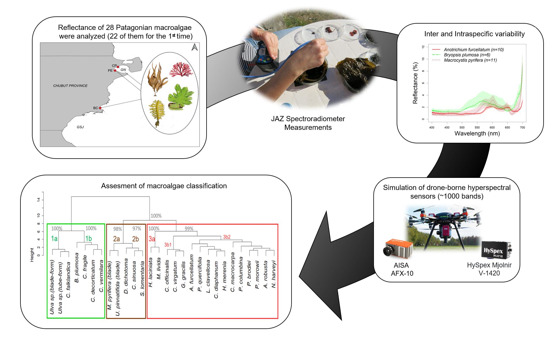
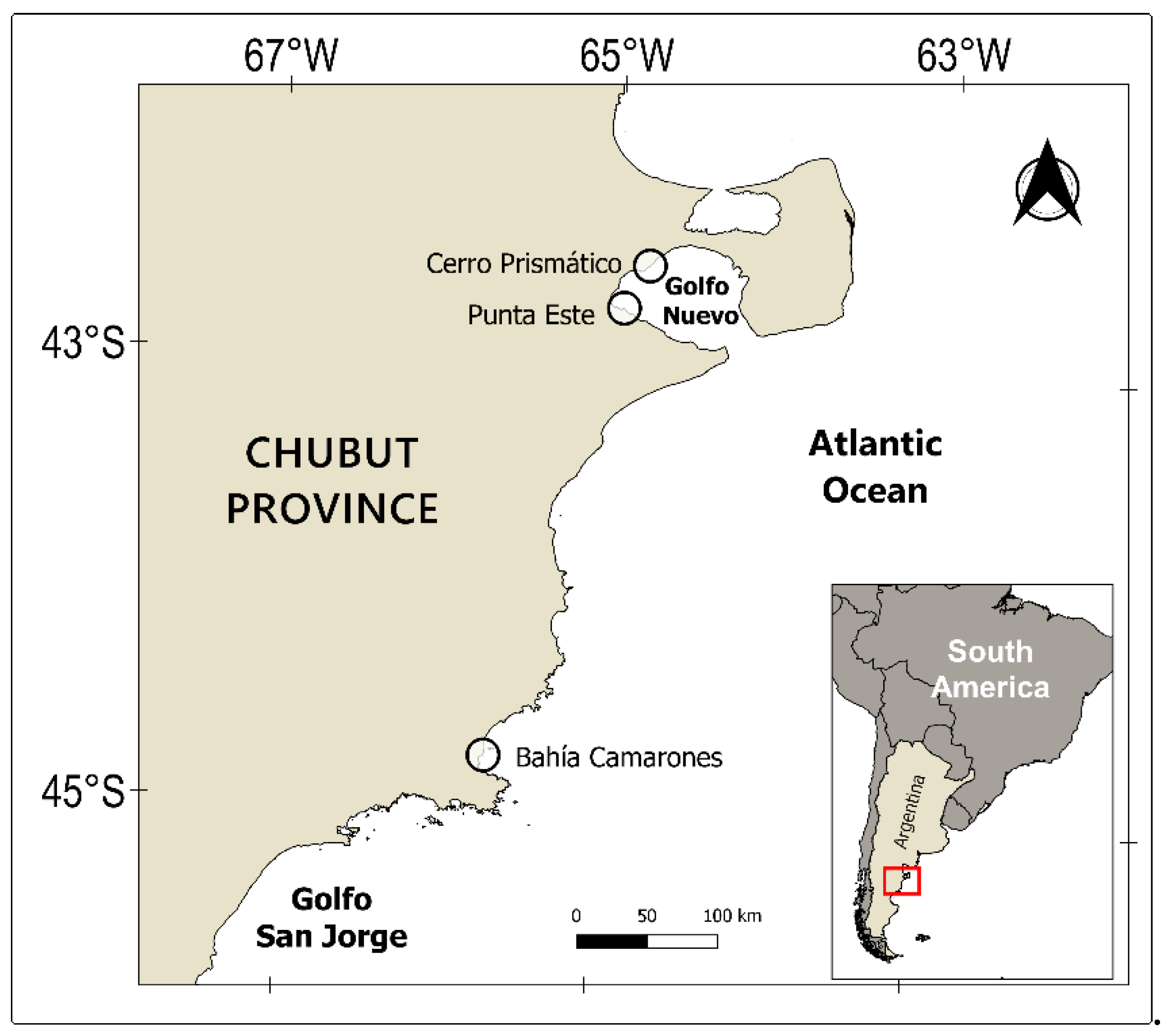
2.1. Study Area

The Patagonian central and southern coast is known for the diversity and abundance of macroalgae [32,34,46]. There is an increase of more than 50% in algal species richness between 42° and 41° S, consistent with the boundary between the Argentine and Magellanic Zoogeographic Provinces [34]. This breaking point is probably related to some environmental factors as temperature [47].
Reflectance measurements of marine macroalgae were acquired from specimens collected at three different locations: two sites located in Golfo Nuevo (Punta Este, PE, and Cerro Prismático, CP) and one in Bahía Camarones bay (BC), 230 km south from Golfo Nuevo. Both places belong to Chubut Province (North Patagonia, SE Argentina) (see Figure 1).
Golfo Nuevo is a semi-enclosed bay (~180 m deep), of low hydrodynamic regime located between the cold and warm biogeographic regions of the south-western Atlantic Ocean [46]. Average water salinity is 33.7 ppm, with maxima of 34.0 ppm [48,49], and mean sea surface temperature is 15.1 °C, with an average night-day amplitude of 2.1 °C [50]. The benthic subtidal macroalgae of Golfo Nuevo are represented mainly by small-sized species, with the exception of the invasive kelp Undaria pinnatifida, first recorded in this region in 1992 [51]. Since its introduction, this kelp has modified the local benthic communities, causing a decrease in the population of native macroalgae [52], and an increase in invertebrate populations [53].
Bahía Camarones is a very open embayment north of Cabo Dos Bahías, inside the Coastal Marine National Park “Patagonia Austral”. Average shelf water salinity is 33.5 ppm [54] and mean sea surface temperature is 13.3 °C with a night-day average amplitude of 2.7 °C [50]. Its high biodiversity makes macroalgae harvesting an important economic activity in the area [55]. Among the most relevant species with commercial applications are the invasive Undaria pinnatifida for fucoidan production, the red alga Pyropia columbina, collected from rocky intertidal zones mainly for food consumption, and Gigartina skotsbergii and Gracilaria gracilis, used to extract polysaccharides of high commercial value [32]. The subtidal zone is also characterized by the presence of Macrocystis pyrifera kelp forests with both great ecological and economical value [56].

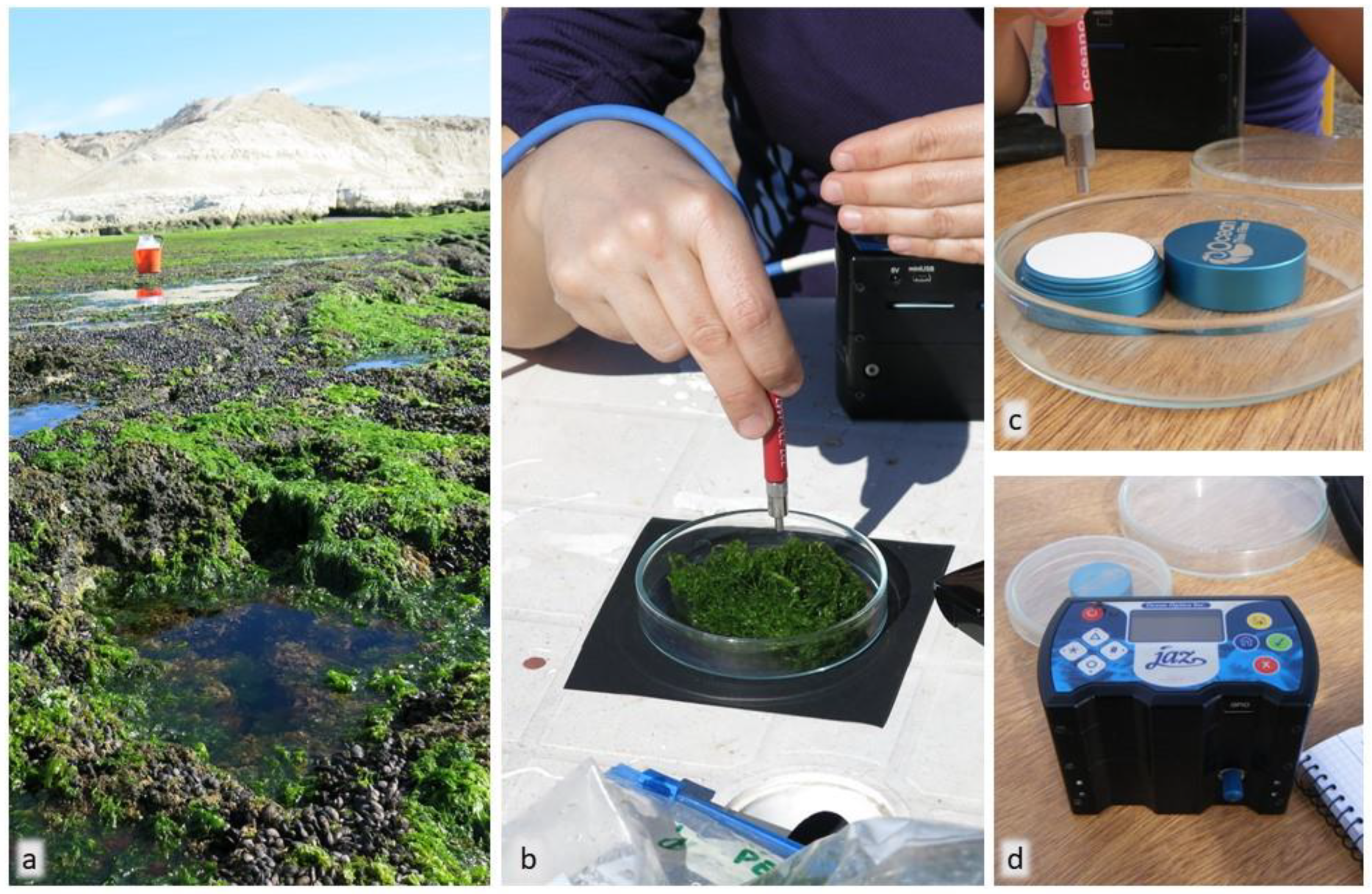
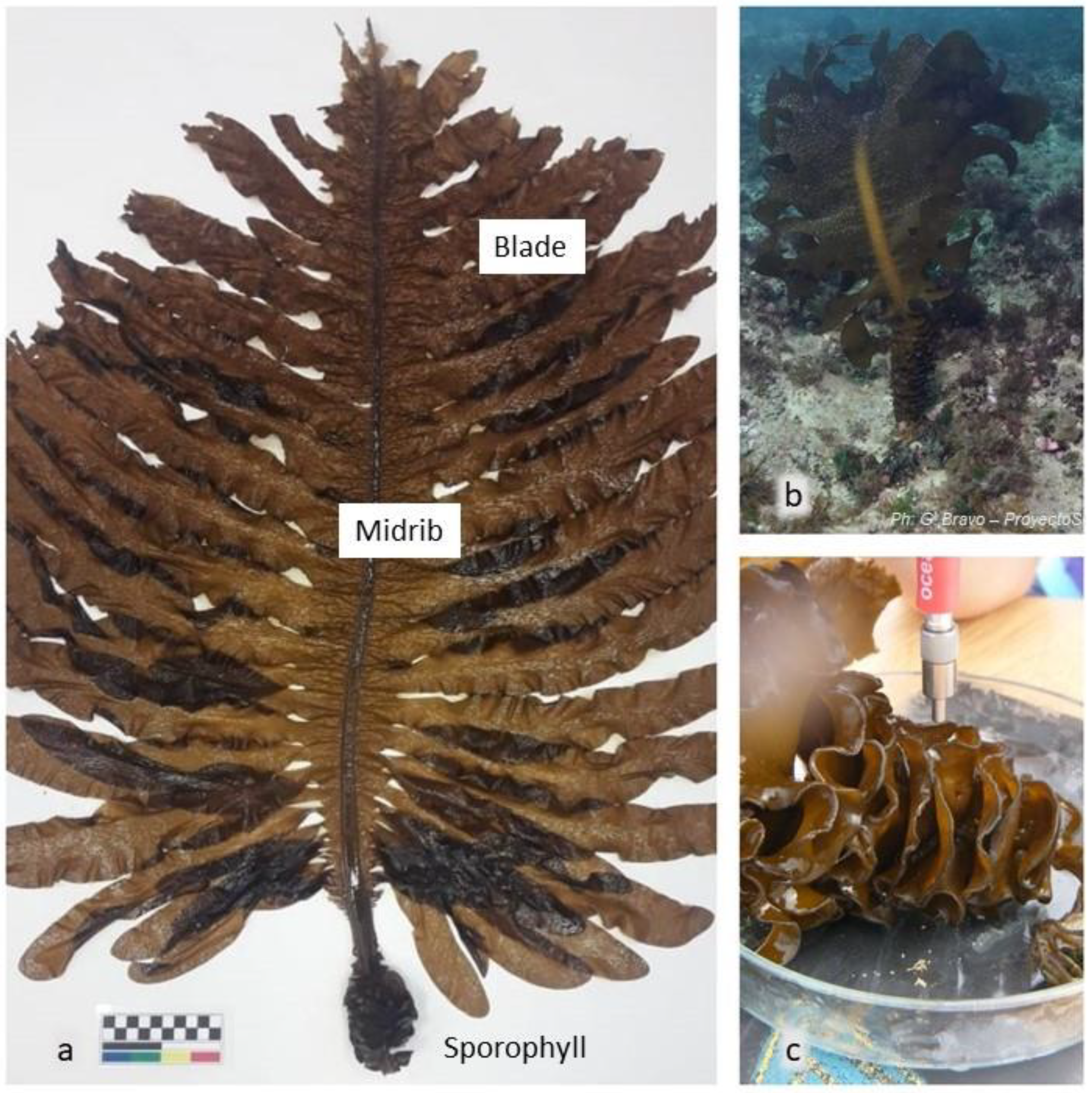
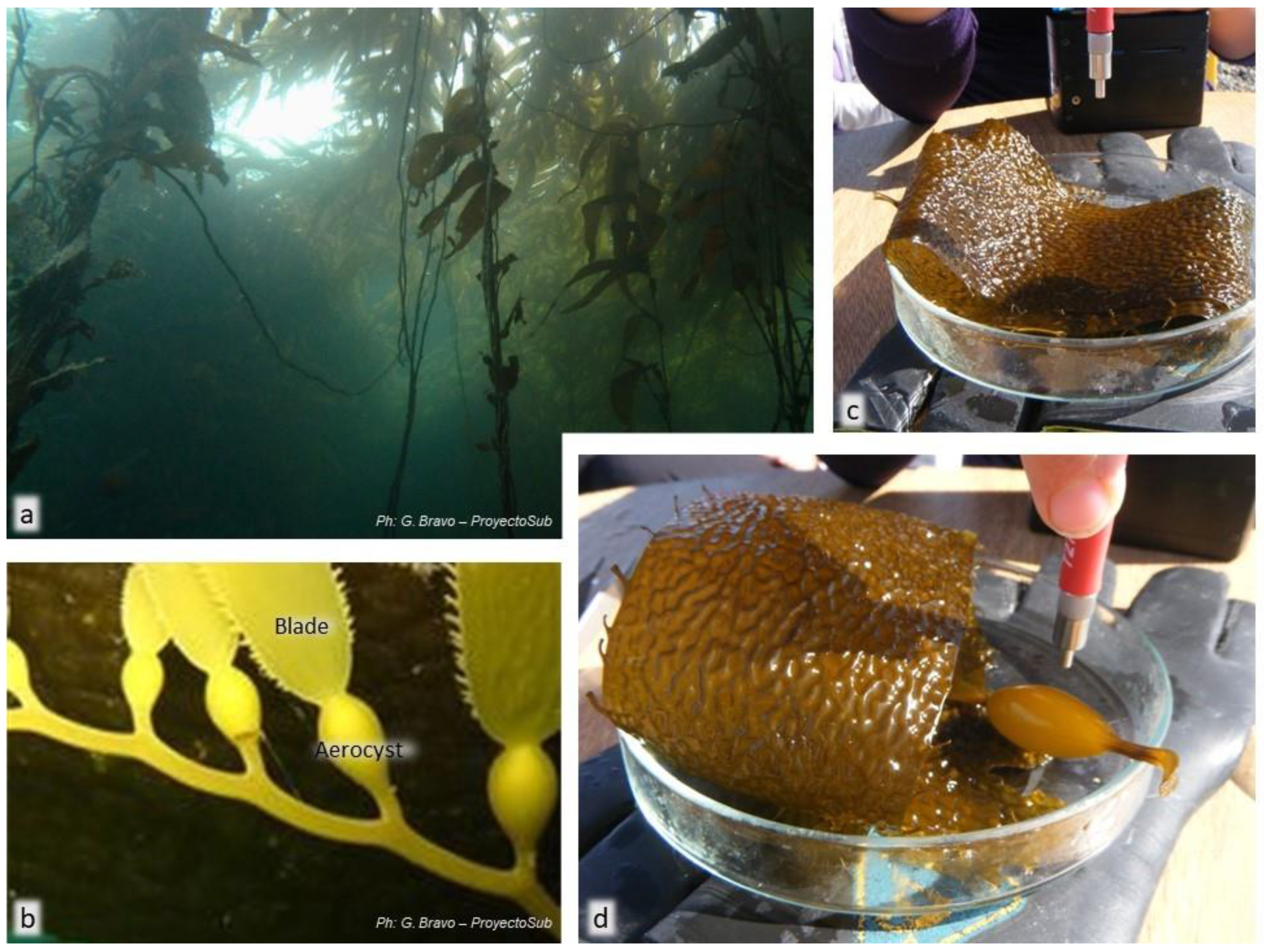
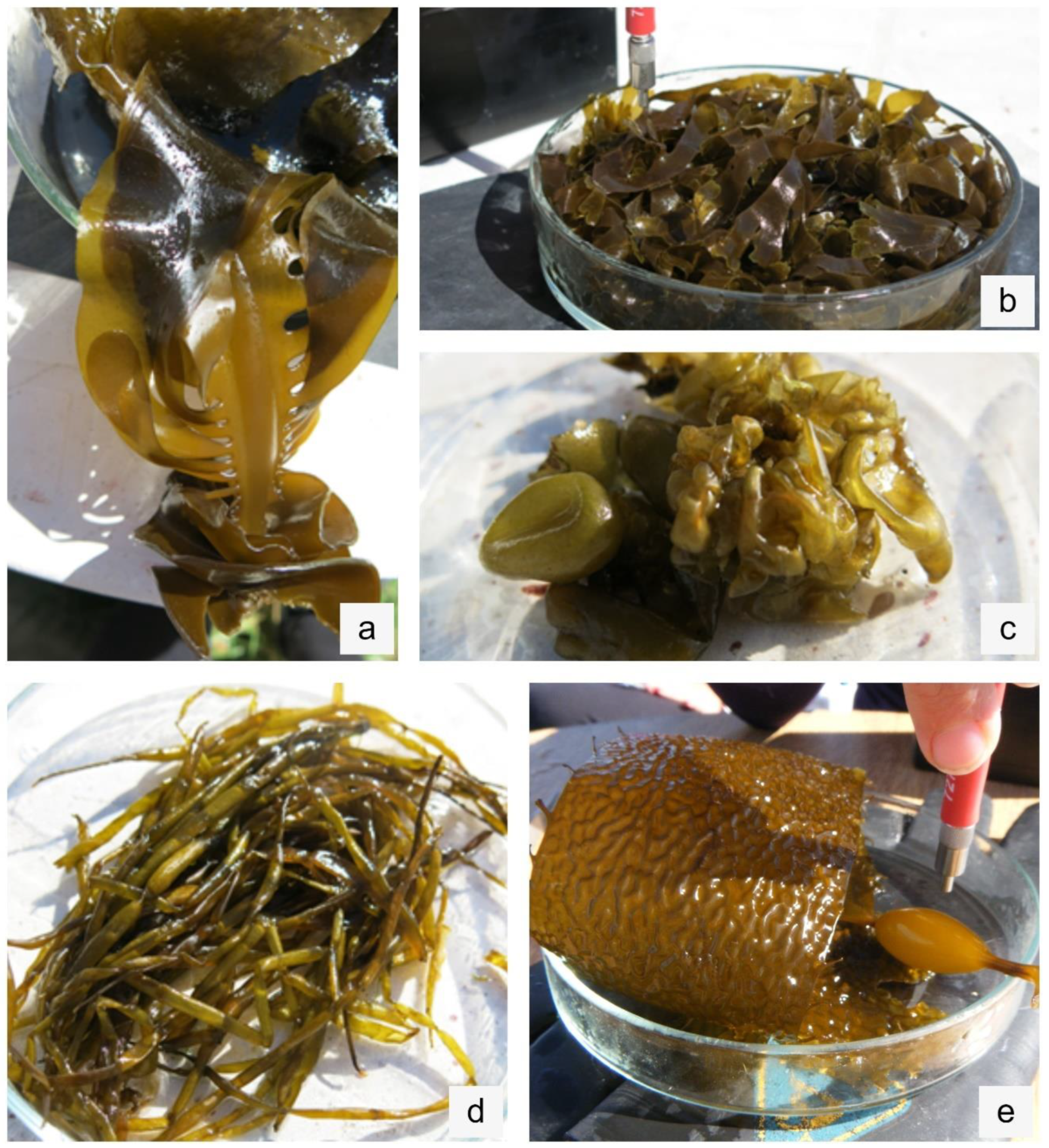
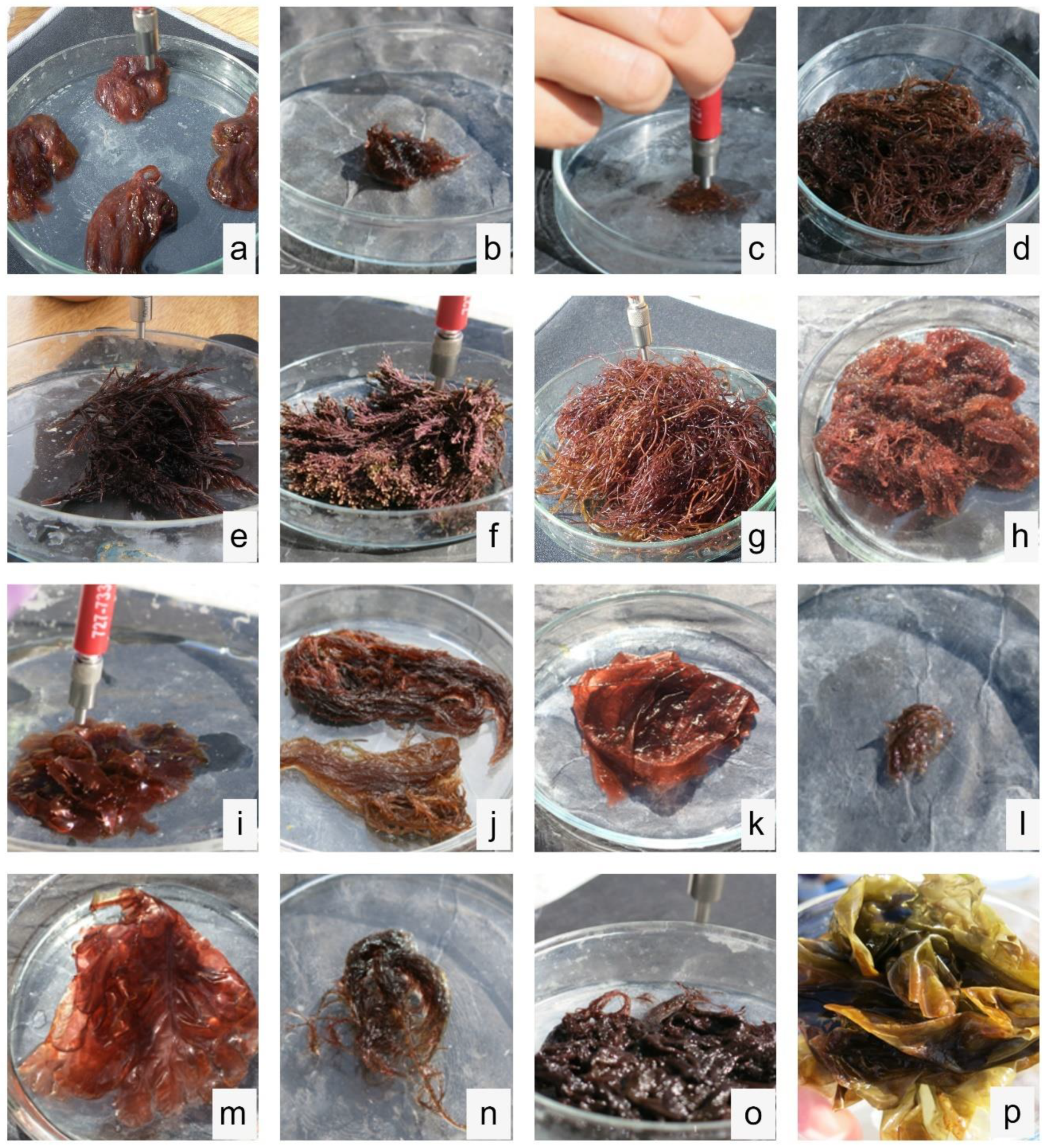
2.2. Sample Collection, Identification and Handling

Benthic marine macroalgae samples were collected during a total of 5 sampling days, (18 March and 14 April 2015 and from 12 to 14 September 2018) and included 28 species of coastal macroalgae (5 brown, 7 green, and 16 red) (see Table 1). The sampling period was determined mainly based on equipment availability, weather conditions (sunny days without wind), and tidal regime (low tides). A specific sampling design regarding dates was not possible, but the possible effects were taken into account. Samples were collected manually from the intertidal coastal zone and natural tide pools, and by diving from subtidal areas, between 1.5 m and 6 m (Figure 2a).
Algal species were identified in the laboratory to the lowest possible taxonomic level. Species names and taxonomic classifications were validated with AlgaeBase [31]. Specimens collected at BC were measured spectrally in situ, while some specimens collected at PE and CP were measured spectrally mostly ex situ due to sampling time constraints. Specimens were stored overnight, for later measurements, in tanks with filtered seawater and with a controlled environment: constant aeration, temperature (15 °C), and photoperiod (12:12). In both cases, samples were stored, and their spectra were measured once again the following day to compare the results.

2.3. Spectral Data Collection

Sample reflectance spectra were measured using a handheld JAZ spectroradiometer (Ocean Optics Inc., Orlando, FL, USA) attached with a QR400-7-VIS-BX reflection probe (Ocean Optics Inc., Orlando, FL, USA) (Figure 2d). JAZ spectroradiometer measures reflectance in 1/3 nm sampling intervals in the spectral range from 350 nm to 1100 nm; however only the wavelengths in the range 400–700 nm were used for this study, spanning the spectral range of photosynthetic active radiation (PAR), because outside that interval either the signal to noise ratio was too low or a number of conditions such as the presence of a water layer attached to the specimen surface introduced further uncontrolled variability in the data. Reflectance measurements were automatically calculated by the instrument as an average of three consecutive reflectance measurements. In order to obtain a smoother reflectance curve, each reflectance spectrum was further applied a moving average (boxcar) of width 5 values.
Reflectance measurements were performed outdoors, using solar light, and under clear sky conditions, between 12:00 am and 16:40 pm local hours. Samples were set on a Petri dish placed over a black background and extended evenly covering the entire dish (Figure 2b and Figure A4, Figure A5 and Figure A6). In the case of kelps, measurements were performed directing the JAZ fiber optics to different parts of the thallus (blade, stipe, and aerocyst for M. pyrifera and blade midrib and sporophyll for U. pinnatifida) (Figure 3 and Figure 4). In order to ensure the quality of the final reflectance spectra for each sample, and to avoid accidental variations in natural illumination, reference whites (Spectralon of polytetrafluoroethylene–PTFE–diffuse reflectance standard, having uniform spectral reflectance >99% in all our spectral range) were used for calibration prior to each set of measurements and, whenever thin clouds were present new reference whites were measured and their values were checked in post-processing (Figure 2c).
Sample reflectances were measured at different times. Some of them were acquired in situ right after sample collection. Many of them, however, due to time limitations, were stored overnight and their spectra were measured the next day.

2.4. Data Analysis

For each sample, several consecutive measurements (usually 5–10, each of them already a filtered average automatically computed by the JAZ spectroradiometer; see Section 2.3 above) were combined to reduce the noise and rule out accidental errors. The white reference spectra, taken at the beginning of each measurement, were used, when available, to recompute spectral reflectances. Thermal noise or dark current, DS, was estimated directly from each spectrum recorded, S, as the lowest signal in the range from 1000–1100 nm (where the digital counts are negligible, partly because of atmospheric water vapor absorption), and the same was done for the white reference spectra, R, obtaining DR; the sample spectral reflectance r was calculated as:
r = 100 × (SDS)/(RDR)
Finally, each species reflectance spectrum was computed as the median of all the sample spectra, and also the interquartile reflectance range was computed in order to characterize the population variability.
All statistical computations and plotting were performed with the statistical software R [57].

2.5. Spectral Classification

The spectral library was used to simulate the reflectances that would be measured by two hyperspectral sensors, the AISA AFX-10 [23] and the Hyspex Mjolnir V-1240 [24], both of which can be borne in unmanned aerial vehicles (UAVs) due to their light weights (2.1 kg without gimbal, or 4.8 kg with it, and <4 kg, respectively). Both systems cover the VIS-NIR spectral range from 400 to 1000 nm. The AISA AFX-10 has 224 bands, a spectral resolution of 5.5 nm spectral sampling 2.68 nm, and 1024 spatial pixels. The HySpex Mjolnir V-1240 has 200 bands, a spectral resolution of 3.0 nm, and 1224 spatial pixels. These simulations do not include any atmospheric effects, so they would correspond to very close observations or to perfect atmospherically corrected hyperspectral measurements.
Reflectance spectra in our library were subsampled to the bands of these two hyperspectral sensors, assuming that the bands are equally spaced and have a fixed spectral bandwidth of ~3.4 nm and ~2.7 nm, respectively. So, the first sensor acquires data in 112 bands between 400 and 700 nm and the second one in 100 bands in the same spectral range. Every reflectance spectra in the library was subsampled to simulated sensor bands by averaging the median spectral reflectance inside each band of the sensor.
Prior to the classification, the simulated band reflectance values in each spectrum were standardized, subtracting the mean reflectance in the interval of 400–700 nm, and then dividing by the standard deviation in that same wavelength interval (following [58]). This standardization was used to highlight the shape of each spectrum (its crests and droughts) above the actual reflectance values, making them more amenable for comparison.
On these standardized simulated spectra, an unsupervised classification using hierarchical cluster analysis (HCA) was performed using each of the subsampled spectra as an element of the classification. Dissimilarity between spectra was determined using Euclidean distance, and the cluster was built with complete linkage. The hierarchical relationships between different sets of data in the spectral library were finally shown in a dendrogram.
The dendrogram structure may be sensitive to the particular selection of samples being classified. In order to assess its robustness, a multiscale bootstrap resampling algorithm was used to calculate the p-values associated with each cluster, i.e., the probability of all the species in that cluster being grouped together, despite the presence or not of other algae in the total classified set. The clustering dissimilarities were computed from correlations (which is equivalent to using Euclidean distances, given that spectra had been previously standardized) using the algorithm described in [59] (and implemented in the R package pvclust).
Having a pre-classified spectral library is useful to perform the classification of new measured reflectance spectra based on their similarity to known ones. Once a distance has been identified that provides (as we will show) a robust meaningful cluster (the Euclidean distance applied to the standardized spectra), that same distance can be used to classify new data using a minimum distance classifier [60]: given a new spectrum, a set of distances to every endmember in the library was computed, and the spectrum ascribed to the class of the endmember at a minimum distance to it.
The performance of this minimum distance classifier was tested in two ways: using spare measurements of 9 different species made at different times than those used to build the library (e.g., a reflectance spectrum of Codium vermilara acquired in 2018, being the C. vermilara spectral signature in the library constructed out of 2015 sample measurements), and using all the measurements available, including those used to build the library. While the first method is a truly independent validation of the classification, the second one was used to assess the classification capability of the library for all classes.

2.6. Feature Identification

When classifying specimens using reflectance spectra, one should explain which bands or wavelengths were influential in the classification. Based on the hypothesis that reflectance spectra are determined to an extent by pigment absorption, we performed an independent component analysis (ICA) to identify the basis of absorption patterns acting in the library. To separate the contributions from different pigments the reflectance spectra were first transformed to apparent absorbance spectra (A) using a logarithmic transformation [61]
A = −log(r)
where r is the reflectance value in each spectral band.
This apparent absorbance can be expressed as the sum of the apparent absorbance patterns caused by the different pigment groups in the tissues. Independent component analysis is arguably the most widely used blind source separation technique [62]. It extracts individual signals from additive signal mixtures, based on the assumption that different physical processes generate unrelated responses. In particular, the fastICA method used here maximizes the neg-entropy of the components mixture and uses a fixed point iterative approximation that makes it converge very fast to the solution; we used the fastICA implementation in the R package “ica” [63].
Each independent component is computed as a linear combination of the library spectra, with different weights given at each spectral band. Thus, following [64], we computed the importance of each band as the average of the absolute values of the weights given to the original data, and compared the positions of relative maxima of that importance measurement with the absorption bands of characteristic pigments.

3. Results and Discussion

In this section, we present the main results of our research, starting with a comprehensive description of the spectral library and then the main result of this article, namely, its cluster classification and its use in the classification of newly acquired reflectance spectra. This will be followed by an analysis of how all that could bring an advantage to actual field campaigns using drone-borne hyperspectral sensors.

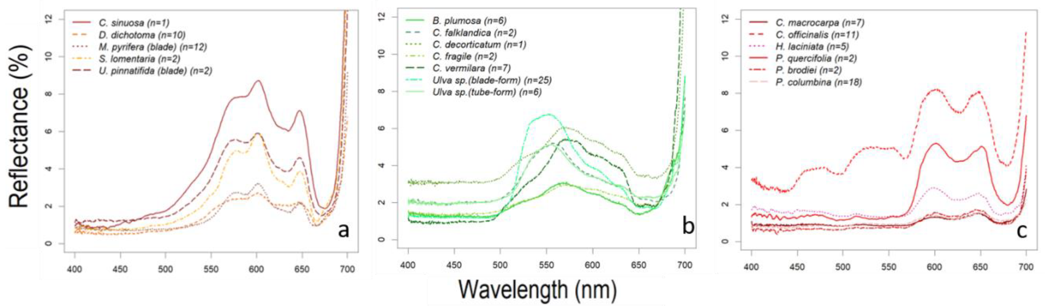
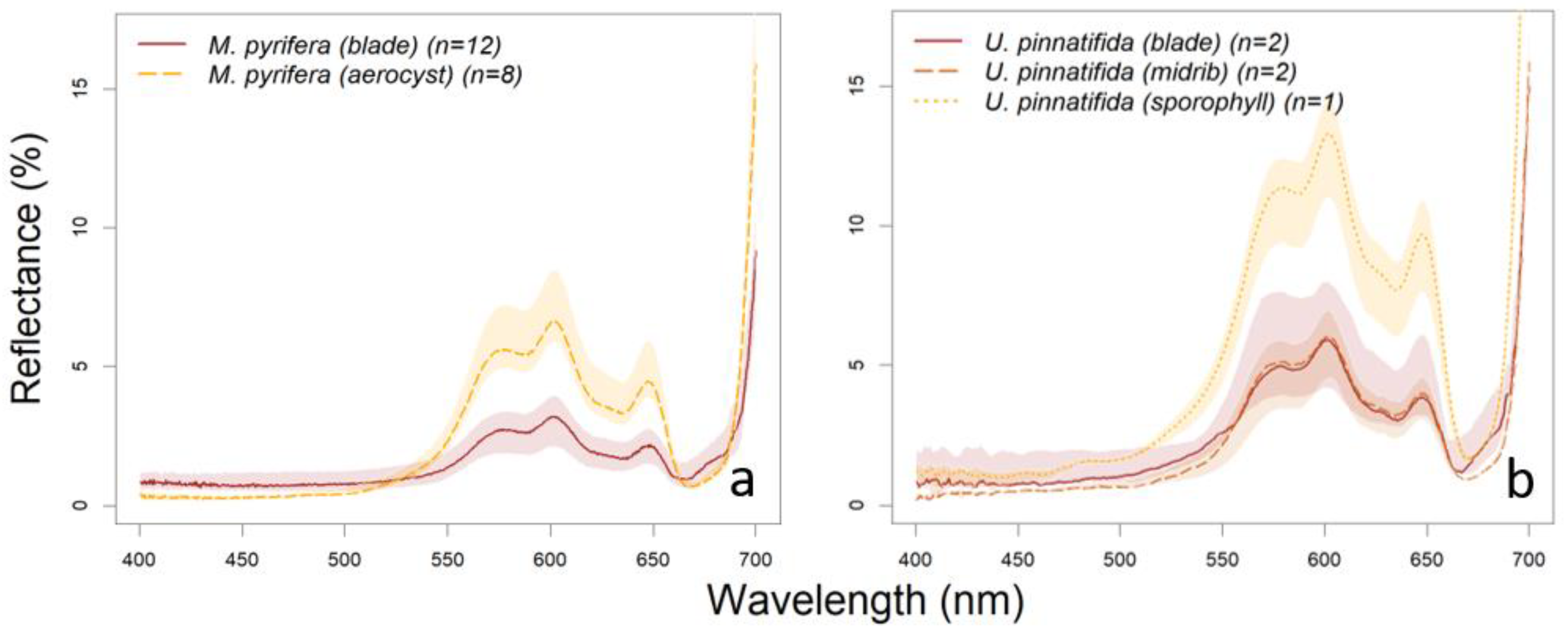
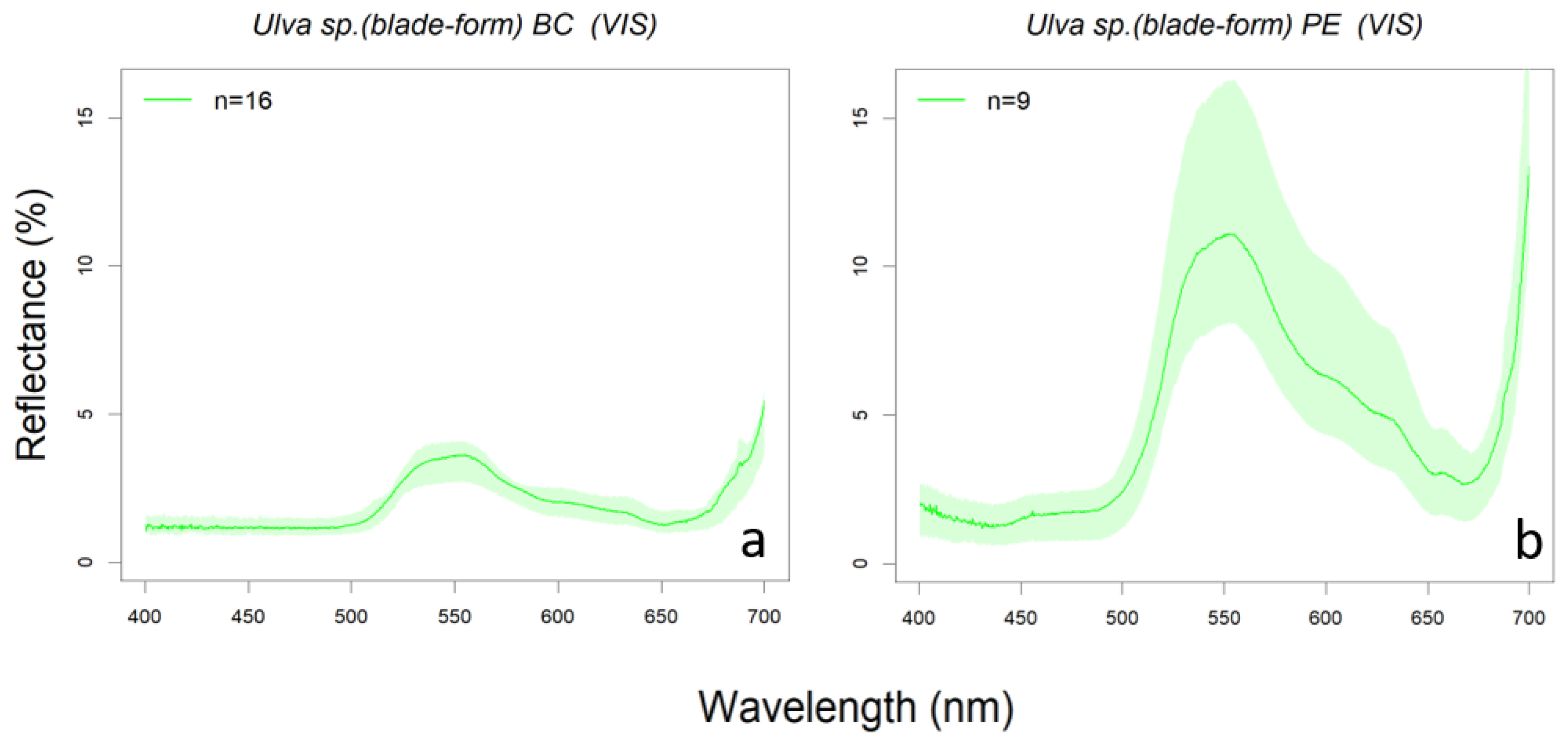
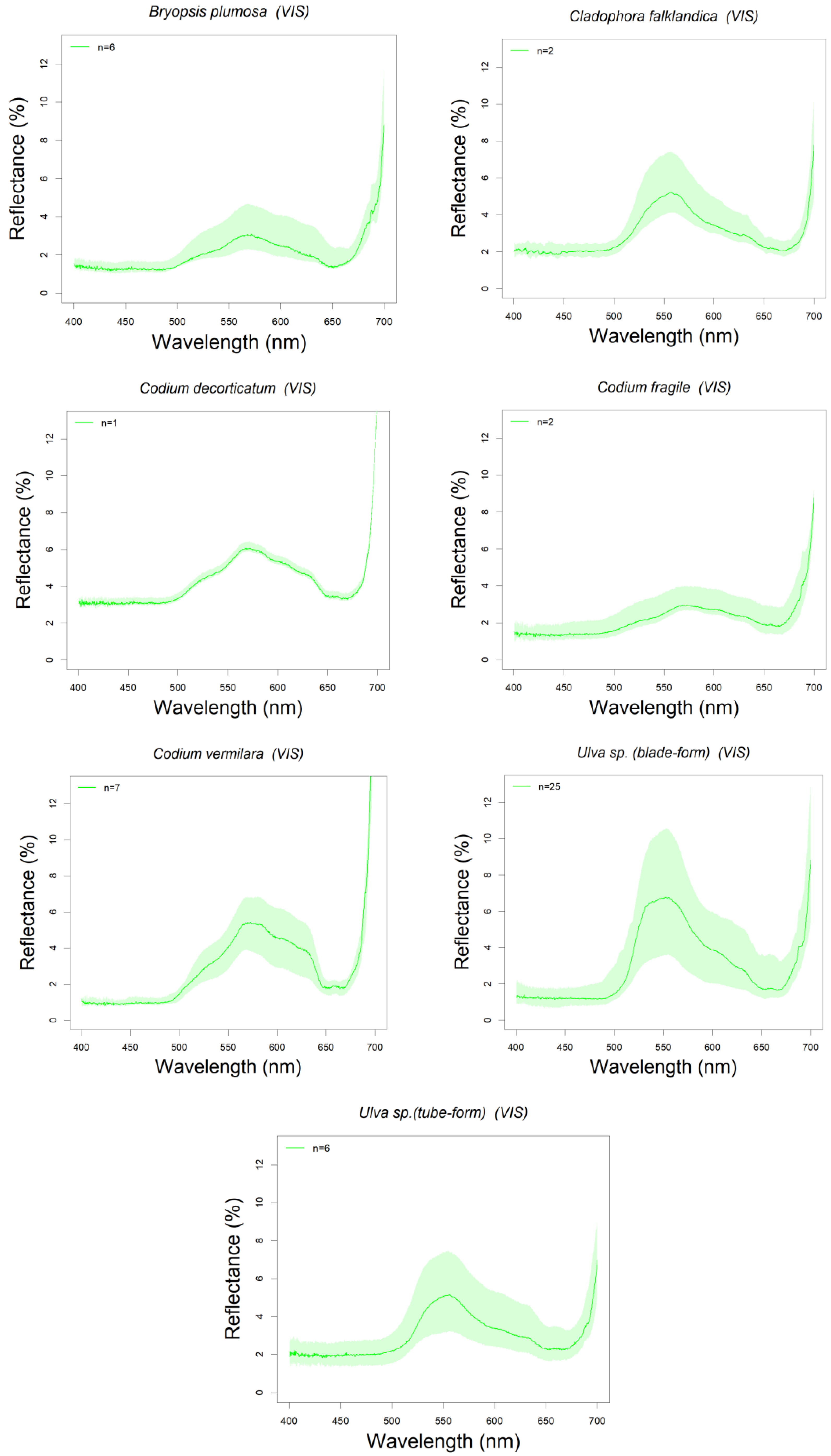
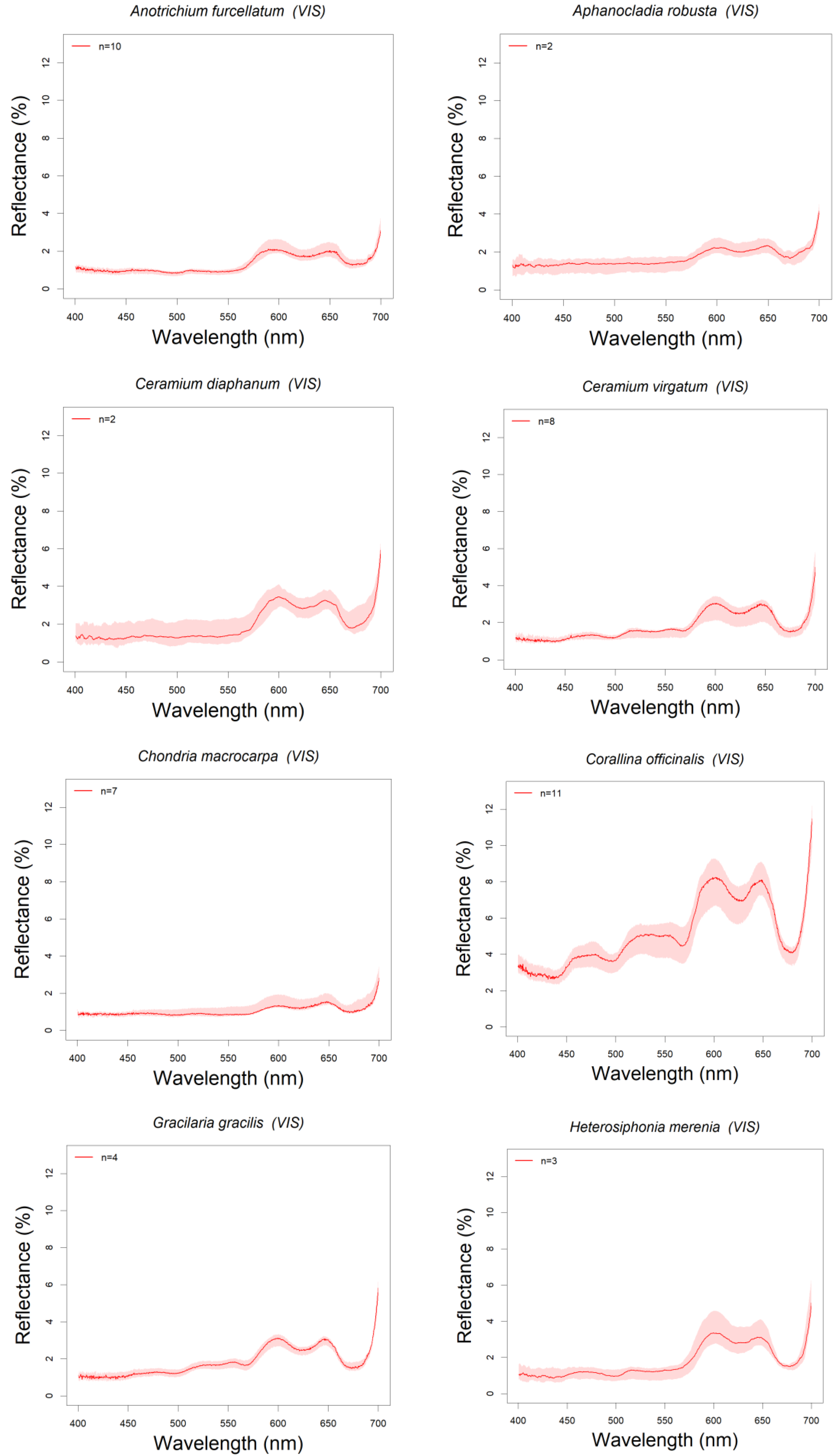
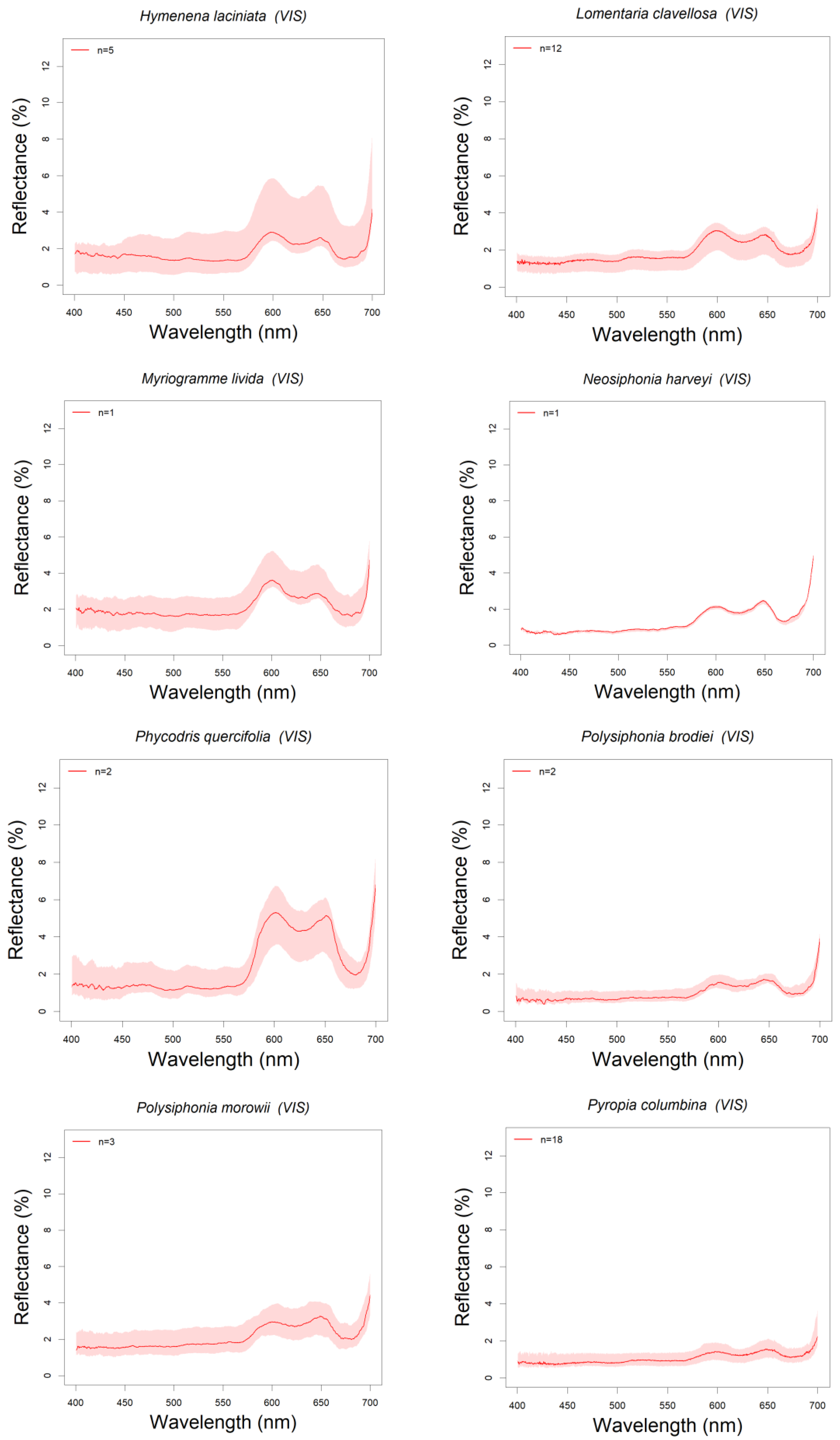
3.1. Library Description

Reflectance spectra of 28 algal species found in Northern Patagonia (Argentina) have been analyzed and classified: five brown (Phaeophyceae, n = 27 specimens), seven green (Chlorophyta, n = 49), and 16 red (Rhodophyta, n = 91) (see Table 1). All these spectra are summarized in the Appendix A, ordered by algal group and showing the reflectance spectra in the visible range (400–700 nm). All the plots include a shadowed area around the median reflectance spectrum indicating the intra-specific variability (upper and lower quartile range) (Figure A1, Figure A2 and Figure A3).
Reflectance measurements used to characterize a species are the reflectance spectra minima (or reflectance troughs), corresponding to absorption bands of the pigments it contains, and maxima (or reflectance peaks), corresponding to non-absorbing bands between them in which light is reflected by tissular structures. In what follows, these features will be described for the specimens of the three main groups in the library.
Brown algae (Phaeophyceae):
Most brown algae showed reflectance peaks around the 580, 600 and 650 nm wavelengths separating the reflectance troughs (absorption bands) around 670–675 nm, 582–596 nm and 630–635 nm (see Figure 5a). These reflectance peaks correspond to the intervals between the absorption bands of photosynthetic pigments characteristic to Phaeophyceae (brown algae) [26,65]. The absorption band around 580 nm corresponds to chlorophyll a (hereafter Chl a, that also absorbs around 673–675 nm), those around 600 and 650 nm to chlorophyll c (hereafter Chl c) and fucoxanthin that also absorbs blue-green light between 400–560 nm [66]. Thus, the absorption bands at ~540 and 580 nm are mainly influenced by fucoxanthin absorption (in vivo maxima 498–500, 540, and 580 nm). This is the major light-harvesting complex of brown algae [67,68] and all the species here studied showed these reflectance troughs and peaks characteristic of this taxonomic group. Among the spectral reflectance peaks found for each species Colpomenia sinuosa, in particular, showed the highest spectral peak reflectances with median values reaching 9% at 600 nm (see Figure 5a and Figure A1). Although only one specimen was measured (Figure A4c), and thus intraspecific variation cannot be assessed, these reflectance values agree with those found by other authors [26,69].
Regarding intraspecific variability, there are two main sources: on one hand, there is a natural variability that could be reflected in variations of cell arrangement, tissue thickness, gas content, chloroplast density, as well as pigment content that varies as a response to light availability or phenological stages [70,71,72]. On the other hand, there are some algae groups that present a complex structure with a clear differentiation of their tissues, as occurs in kelps (a group of brown algae belonging to the Order Laminariales) [73].
One of the species whose reflectance spectra shows higher variability is Dictyota dichotoma. Although its reflectance has not been reported in the literature, the spectra of two species in the same genus, D. mertensi and D. ciliolata [74], showed similar spectral reflectance patterns (see Figure 5a and Figure A1). D. dichotoma is a medium to small sized algae (around 0.1 to 0.2 m in length) that can be found from intertidal pools to subtidal environments. Specimens sampled in this work were taken from two different locations and also at different times, therefore were exposed to different environmental conditions (as temperature, nutrients and irradiance), which could explain the variations on reflectance values found for this species. Other species that presented a high intraspecific variability was M. pyrifera, specifically in its blade reflectance (Figure 4), although the median spectra agree well with earlier results reported in the literature [75,76]. This is a large subtidal species, (1 to 15 m long in North Patagonia) and characterized by different tissular structures with different functions, such as the support and and its aerocysts serve to its floatability, reaching the sea surface [56]. Its aerocysts serve to its floatability, reaching the sea surface. Blade samples taken from BC were measured at different lengths of the thallus (5 m long, in average) and were probably exposed to different environmental conditions, decreasing the exposure to radiation from the upper to the lower parts of the thallus. This could explain the intraspecific variation in M. pyrifera blade spectral reflectance (Figure 6a).
Part of the spectral variability in kelps is related to the different tissues that form their thallus. The reflectance spectra of M. pyrifera, aerocysts and blades have the same overall form, however, reflectance is higher for aerocysts (see Figure 6a). The blade tissue is thinner and with more pigment concentration. The higher reflectance of the aerocyst could be explained not only by the different size and pigment concentration in its cells, but also by its anatomy showing an internal cavity allowing plants floatability [77,78]. Moreover, aerocysts and stipes play a structural role and transport compounds along the thallus through medullar cells (hyphae) that are less pigmented, resulting in less absorption in the visible wavelengths [78]. The same pattern was found for U. pinnatifida whose sporophyll, blade, and midrib spectral reflectances have the same overall form, although higher values for the sporophyll than for the other two tissues. Blade’s lower reflectance could be explained also by its thinner structure and higher pigment concentration than the other parts of the thallus [73,79,80] and the higher spectral variability (related to the midrib and sporophyll) can be attributed to its different stages. Undaria’s midrib is characterized mainly by medullar cells which are less pigmented and with a predominantly longitudinal orientation, and several cortical layers forming a rigid supporting tissue [81], that would be responsible for its higher reflectance compared with the blade [79,80]. Finally, the highest peak reflectance found in the sporophyll (Figure 6b), could be related to the presence of less pigments, but also to it being a thicker tissue with reproductive function.
Green algae (Chlorophyta):
Most green algae showed a reflectance peak in the green region of the visible spectrum, around the 550–590 nm, varying from the 555 nm of Ulva spp. (both, blade and tube forms, the latter previously reported as Enteromorpha sp.) to the 585 nm of Codium vermilara. The 550–590 nm reflectance peak characteristic of this group is caused by the nearby absorption bands of chlorophyll b (hereafter Chl b), a pigment specific of green algae, one in the 468–478 and another in 645–659 nm [72,82]. The presence of Chl b in this group shifts the reflectance peak towards shorter wavelengths (towards the green) and narrows it. The lowest peak reflectances were recorded in Bryopsis plumosa and Codium fragile (below 4% at maximum), whereas Ulva sp. (blade-form, above 7%) and Codium decorticatum (above 6%) showed the maximum peak reflectances (Figure 5b). Reflectance measurements of green algae can be separated in two different subsets, one presenting the main reflectance peak at 600 nm (B. plumosa and Codium spp.), and the other presenting the reflectance peak at 550 nm (Ulva spp. and Cladophora falklandica). Certain green algae contain a specific ketocarotenoid, siphonaxanthin, associated to siphonein to help absorbing the available green and blue-green light (500–550 nm), as Bryopsidales Order [83,84,85] to which the first subset species belong: B. plumosa and Codium spp. This latter genus includes the three Codium species recorded for north Patagonia [32,86]: C. fragile, C. vermilara and C. decorticatum. Their spectra differ in the relative depths of the two main Chl b absorption bands, whose reflectance minima are approximately the same for C. decorticatum, while C. fragile absorption band is in the red, and C. vermilara has the blue absorption band deeper (although the red one is also deeper than C. decorticatum’s) (Figure 5b). While C. decorticatum can be found only in the subtidal zone, the other two species can be found in a wider gradient of environmental conditions, varying from intertidal tide pools to shallow subtidal. Thus, spectral patterns could be explained in terms of the variation of the environmental conditions requiring a different balance of photosynthetic pigments according to its habitat. The spectral absorption features of Ulva sp. (blade-form) are consistent with those presented in [26]. However, these specimens studied in our work showed a small reflectance peak visible between 520 and 570 nm (Figure 5b). This discrepancy could be attributed to uncertainty in expert classification of the species actually sampled. The reflectance spectra of the genus Bryopsis follow the same patterns shown in [69], but do not present the reflectance peak at 680 nm observed in the spectral signature of B. corticulans [87]. The spectral signature of Cladophora falklandica presents the reflectance peak at 550 nm (Figure 5b) more marked than the C. glomerata [45]. As occurs with Ulva sp., these differences could be attributed to species differences within the same genus.
Intraspecific variability is especially high for Ulva sp. (both blade- and tube-form), Codium vermilara, and Cladophora falklandica (Figure A2). In particular, Ulva sp. (blade-form) showed such a large intra-specific variability that its upper quartile reflectance reached the 10% (see Figure 7 and Figure A2). A great variability was found between the thallus from subtidal populations of Bahia Camarones and intertidal populations collected in Punta Este, showing the latter a higher reflectance peak at 550 nm. It has been demonstrated that several species with intertidal and subtidal populations do not have unique acclimation to irradiance being shade-tolerant, but can also change their morphology under environmental pressure [88]. Therefore, these spectral reflectance intraspecific variations could be related with different pigment content, responding possibly to seasonal, bathymetric and latitudinal variations.
Red algae (Rhodophyta):
Red algae showed two reflectance peaks in the red region of the visible spectrum, around 600 and 650 nm, and reflectance troughs in blue and red bands: 492–506 nm and 610–630 nm, that corresponds to absorption by phycoerythrin (492–506 nm) and phycocyanin (610–630 nm) (see Figure 5c), the two phycobilins that characterize red algae [26,65]. Most species ranged their median reflectance peaks below 4%, except for Phycodrys quercifolia (peak reflectance 5.3%), although intra-specific variations cause upper quartiles to largely surpass some of these maxima (Myriogramme livida and Hymenena laciniata upper quartiles reach above 5% and 6% respectively) (see Figure 5c). Some species like Chondria macrocarpa, Polysiphonia brodiei and Pyropia columbina showed the lower reflectances (less than 2%) in the blue band, where phycoerythrin absorbs around 500 nm, which is in accordance with higher pigment content (Figure 5c and Figure A3). This could be explained by the higher phycobiliprotein content found in Polysiphonia and Pyropia genera compared with other species [89]. The highest intra-specific variability among the red algae corresponds to Hymenena laciniata (Figure 5c and Figure A3). This is a subtidal species but could be also found on intertidal pools. Specimens here studied (Figure A6i) were collected from tide pools, where they are more exposed to solar irradiance than subtidal populations, and that also varies depending on the intertidal level where they were collected. These factors could change the balance of pigment content in the specimens. The spectrum of Corallina officinalis, has a particularly high reflectance, with a minimum above 3% and a peak maximum of 8% at 600 nm (Figure 5c and Figure A3). The signature of this species showed patterns characteristic of the Corallinaceae group described by other authors [90,91], where R-phycoerythrin and Chl a are the main contributors to light absorption causing a reflectance peak in the blue (437–439 nm), while the highly reflective calcium carbonate skeletons originate an overall increase of reflectance. Other species of some genera such as Chondria, Ceramium, Gracilaria and Polysiphonia have been characterized in [26,92,93] and also showed some similarities with the species we describe (Figure 5c and Figure A3). For the rest of the species of this group presented in this work, we could not find spectral signatures in the previous literature, suggesting that nine genera in the spectral library represent novel information (Table 1).

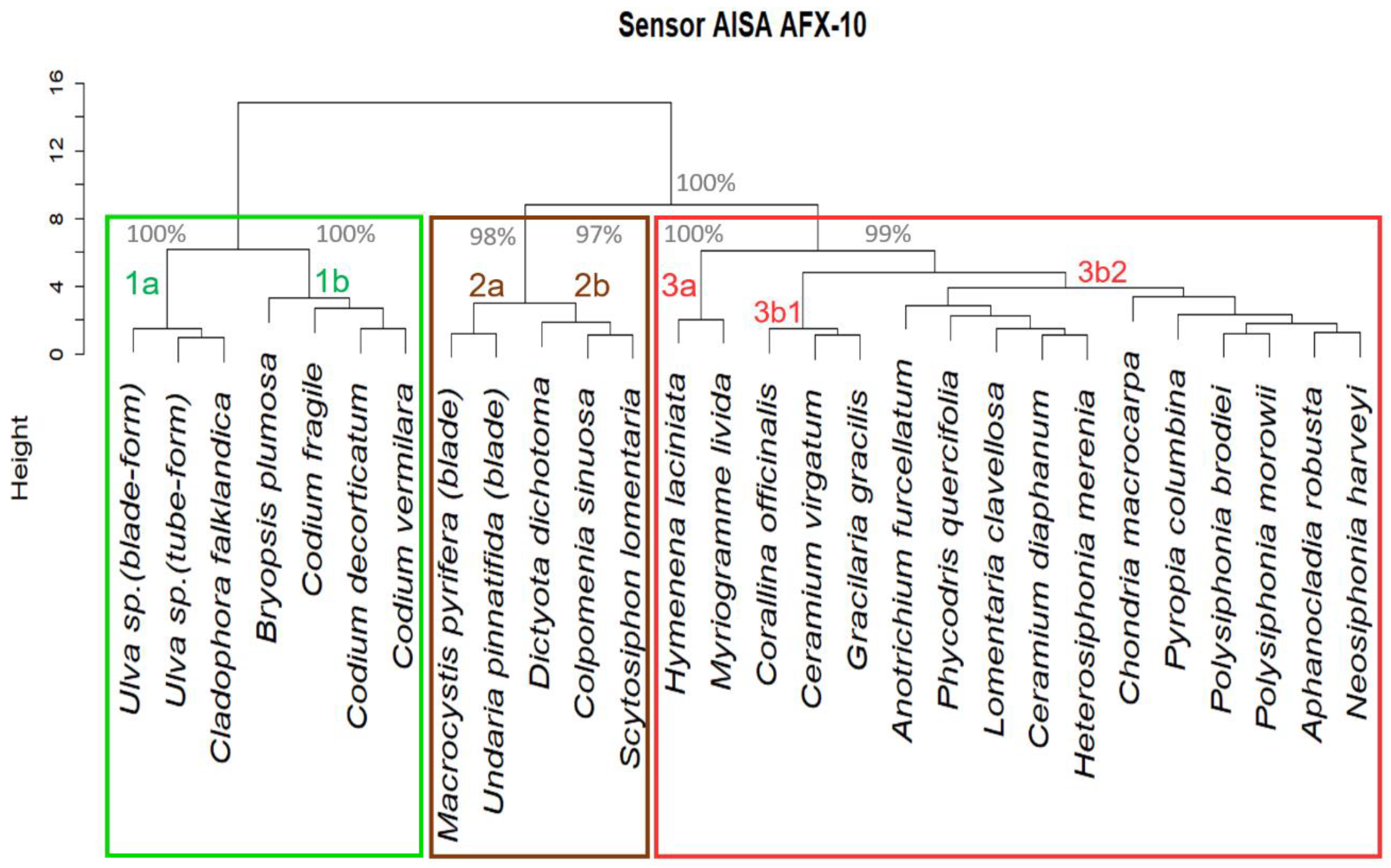
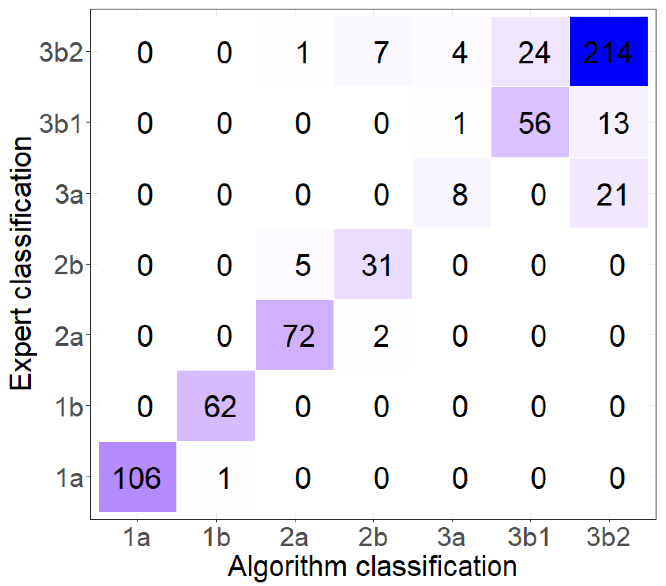
3.2. Algae Group/Classification by Hierarchical Cluster

The cluster analyses of spectra simulated for the two hyperspectral sensors, the AISA AFX-10 [23] and the Hyspex Mjolnir V-1240 [24], showed very similar results. Dendrogram structure is consistent over the two data sets, showing the same grouping of species, thus only the first dendrogram will be described (Figure 8).
The dendrogram presents two branches, one corresponding to the green algae (branch 1) and another one that divides in other two branches, one containing the brown algae (branch 2) and the other one the red algae (branch 3). Each of these branches further splits into two sub-branches labeled 1a, 1b (for branch 1), 2a, 2b (for branch 2), and, 3a, 3b (for branch 3) (Figure 8). The bootstrap analysis of stability of the dendrogram shows that the p-values corresponding to the 1a and 1b, and to the 2 and 3 branches are 100%, that is, irrespective of the subsample of species used in the classification, the spectra contained in those branches always get classified together, thus ruling out the chance effects on the classification. The 2a and 2b branches are thus classified in over 97% of the sampling distributions, as well as the 3a and 3b branches. However, below that division, the subcluster p-values have more diverse probabilities, indicating that especially red algae are more difficult to differentiate.
The first cluster branch in Figure 8 (1) includes the green algae, those with a most noticeable reflectance peak around 550–590 nm, and separates into two sub-clusters (1a, 1b). The first sub-cluster (1a) is composed by the genera Ulva and Cladophora. Despite the first genera has a parenchymatous tissue formed by two layers of cells, and Cladophora falklandica is a uniseriate filamentous species, both genera present a multicellular arrangement with cells well differentiated by the cell wall [32]. The second sub-cluster (1b) is represented by two genus belonging to the Order Bryopsidales whose morphology varies among tubular siphons to highly branched, but all consist of a single undivided cell [94]. When comparing the reflectance measurements of siphonous species and multicellular arrangements, a clear difference in the pigment absorption range is visible. In the second group, the absorbance around 518–540 nm may correspond to siphonaxanthin and siphonein pigment [85,95,96] which are present in Codium (a subtidal genus) light-harvesting complexes that are responsible for enhanced absorption in the green region [97]. The siphonaxanthin-Chl ab proteins allow enhanced absorption of blue-green and green light, the predominant light available in deep ocean waters or shaded subtidal marine habitats [97]. This could explain the subsequently two divided leaves as this pigment is absent in species that grow in shallow water (Cladophorales and Ulvales) but is present in all of siphonous species (Bryopsidales Order) [72,84,85,96,98]. Therefore, the difference between the 2 clusters that we observe in green algae (Figure 8, 1a and 1b) may be caused by a combination of different cell arrangements and different pigment concentrations and composition.
Brown algae are grouped in branch 2 of the dendrogram (Figure 8). These algae are characterized by having Chl a and other accessory pigments such as Chl c and fucoxanthin [66,72]. As a consequence, their spectra show greater absorption in the blue and green regions, which could be also enhanced by their thallus morphology and thickness variations among species [99,100]. All these features determine the division of this dendrogram branch into two leaves: one corresponding to the group formed by two kelp species, U. pinnatifida and M. pyrifera (Order Laminariales) (branch 2a in Figure 8), and another formed by non-kelp species (branch 2b). The former ones have a thallus with complex structure (as described in the previous section) and the populations studied are subtidal or, if intertidal, taken from tide pools where they remain submerged. This group has also spectral characteristics with high reflectance in the near infrared region and significantly lower reflectance in the visible [12] which differentiate them from non-kelp brown algae (2% and 3% peak median reflectance, respectively). Moreover, the “kelps” group shows strong absorption in the 500–550 nm spectral region that could be related to a higher concentration of fucoxanthin, and an absorption peak at 630 nm due to Chl c, being more evident in Macrocystis pyrifera [93,101,102,103]. On the other hand, the second “non-kelp” group shows another sub-group represented by one branch with a single species Dictyota dichotoma, and the other formed by two species: Colpomenia sinuosa and Scytosiphon lomentaria. Despite all three species are parenchymatous, they present different morphologies and occupy different habitats [15,32,72]: while D. dichotoma has a dichotomously divided laminar thallus and is mainly found in subtidal habitats, C. sinuosa is saccate and S. lomentaria is tubular, and both develops in the intertidal rocky shores [32,104]. Studies have shown that in thicker thallus the fraction of the absorbed incident light is greater [105,106]. These differences, both morphological and environmental (intertidal and subtidal habitat), imply different received irradiances, suggesting different adaptive responses in terms of pigments balance.
The third cluster of the dendrogram is formed by the group of red algae (branch 3 in Figure 8). As distinctive spectra, they exhibit two characteristic reflection troughs in the visible spectrum, the first of one, related to the absorption by phycoerythrin pigment in 545–565nm, while the second could be caused by absorption of phycocyanin at ~620 nm and ~675 nm [72,107]. The red algae reflectance measurements are consistent in their shapes but variable in reflectance values, reflecting the great diversity in this group [31]. Despite the fact that three sub-clusters can be distinguished in the red algae arrangement, it has not been possible to relate this arrangement to a correspondence in their morphological, taxonomic characteristics or according to their habitats as was possible for the two previous groups. Given that red algae are the most complex group in terms of numbers of species, future studies involving more factors (such as those mentioned above) will probably be necessary to better understand their grouping or eventual rearrangement according to their inter and intraspecific variation.
We have tested the classification accuracy using a validation set of 119 reflectance spectra corresponding to 31 specimens distributed across nine different species in the library. Then, for the sake of completion, we tested the classification accuracy on our entire data set comprising 635 reflectance spectra corresponding to 198 specimens distributed across the 28 different species. The confusion matrix of this complete classification is shown in Figure 9.
The validation set had an uneven sample distribution among the classes, because specimens acquired in both the 2015 and 2018 measuring campaigns, just covered four of the seven dendrogram classes: branches 1b, 2a, 3b1, and 3b2. Nevertheless, the accuracy of this classification was 85.7% with a Cohen’s kappa of 0.809, denoting a good agreement between the expert classification and the library-based classification. When all measured specimens were tested, the accuracy increased to 87.4% and Cohen’s kappa also improved to 0.837, a very good agreement. As expected from the taxonomic and dendrogram stability analyses of the previous sections, the worst classification occurs among the red algae (branches 3a, 3b1, and 3b2). All in all, this means that the probability of having a new spectrum correctly classified in one of these seven classes is greater than 80%.

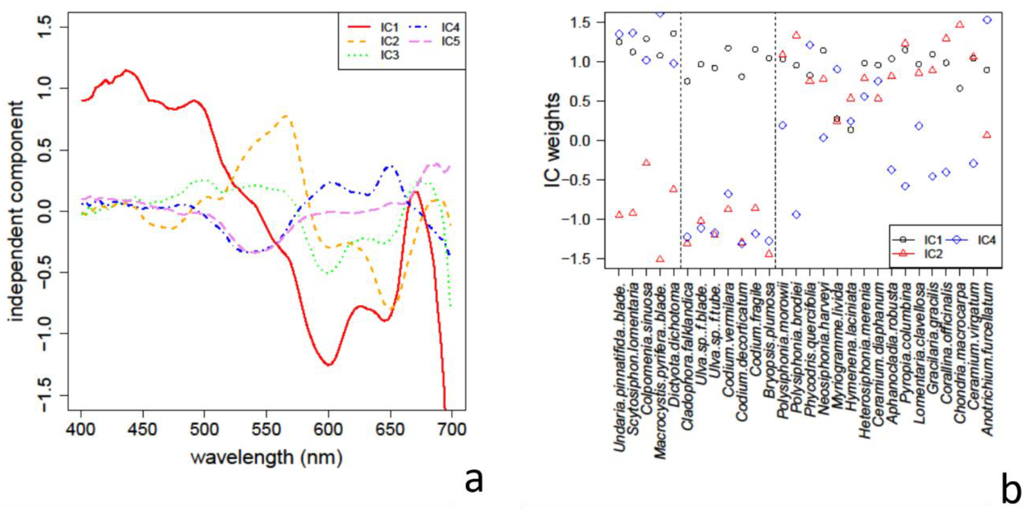
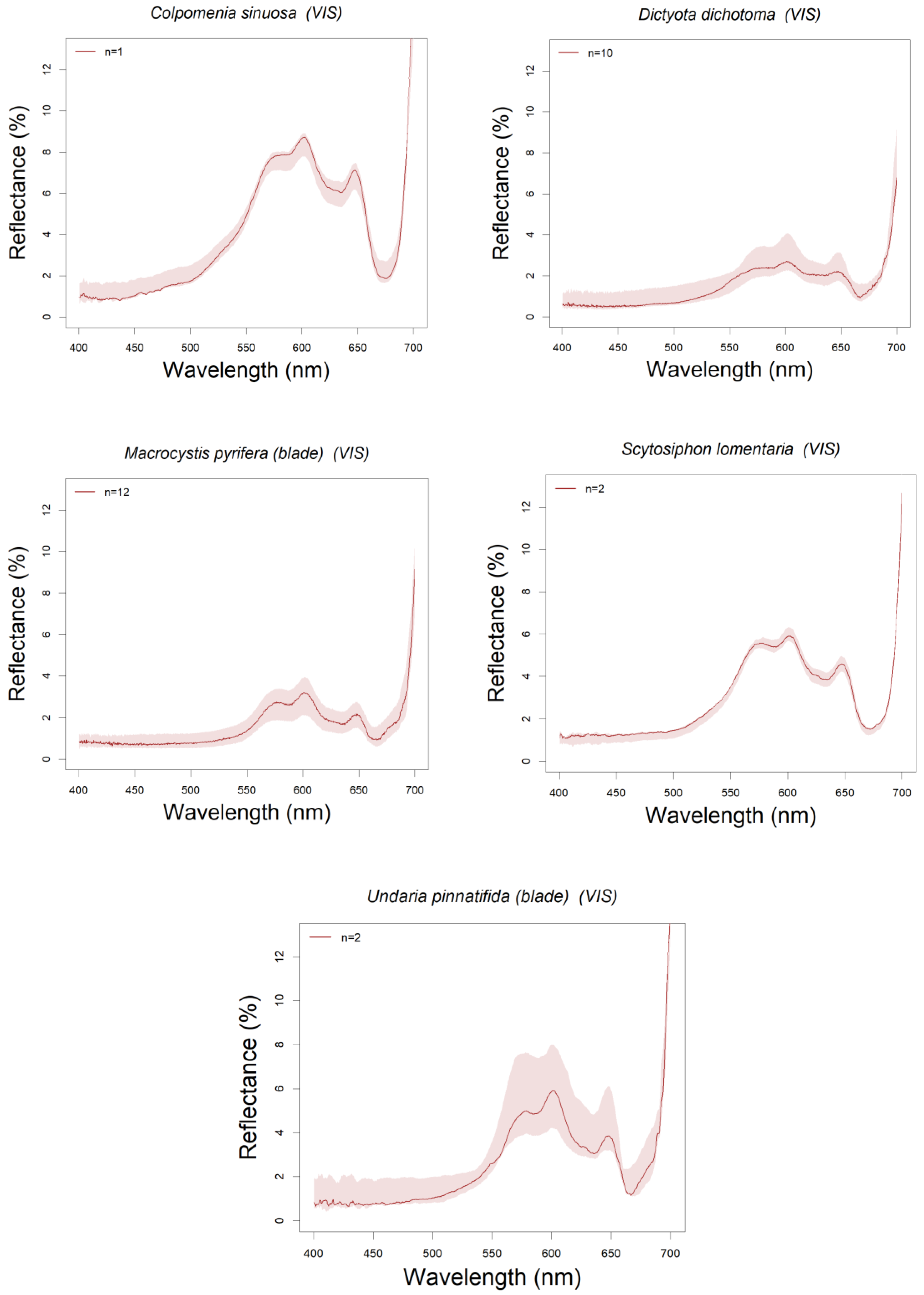
3.3. Absorption Feature Identification

The application of ICA to the spectra in the library identified a number of apparent absorbance features that are depicted in Figure 10a. Although the maximum number of ICs could be the same as the number of spectra (28 in our case), we have checked that with only the five components shown all the absorbance spectra can be computed (with an r.m.s. error less than 5% for all the species, and less than 2% for 22 of the 28 species).
The first IC shows the absorption profile common to all algae, with a wide absorption band in the shorter wavelengths (400–500 nm) and the sharp Chl a absorption peak close to 680 nm (see Figure 10b). The second IC shows an absorption peak around 560 nm and another around 690 nm which are characteristics present mostly in red algae (see Figure 10b). The third IC reproduces again the absorption features of red algae; however, its weight among the species does not follow a recognizable pattern. The 4th IC has relative absorption maxima around 540 nm, 530 nm, and towards the red-NIR edge, where absorption mostly differentiates brown from green algae. Finally, the 5th IC has also a maximum around 540 nm, and a slight maximum around 660 nm. However, its weight among the species does not show a recognizable selection pattern.
The importance of spectral bands computed from the weights matrix used to obtain these ICs, identified the 18 bands (with average absolute weights greater than 2) which are listed here (in parentheses are included characteristic pigments with close absorption bands): 415, 425, 436–450 (Chl a), 463 (Chl c), 471 (Chl b), 492 (fucoxanthin), 549 (phycocyanin), 562 (phycoerythrin), 578, 592 (Chl c), 610, 634 (Chl c), 645, 653 (Chl b), 659, 672, 688, 696. The hierarchical cluster classification obtained restricting the bands to these selected ones, is the same as that obtained using the full 112 bands of the AISA AFX-10 to the level of the branches shown in Figure 8.
The existence of these “influential” spectral bands, their close relationship with absorbance bands of the algae photosynthetic pigments, and their ability to recover the hyperspectral classification, suggest that a similar approach could be used to design imaging campaigns using tunable band sensors (with interferometric analyzers and filters) fitted to these spectral bands.

3.4. Potential Applications and Future Work

In the previous analyses we have described a spectral algal library that can be used to classify hyperspectral reflectance data acquired with a current drone-borne sensor, and have shown how this may work statistically. In what follows, we analyze how practical this approach can actually be in the context of remote sensing, whose goal is to collect and analyze data from a distance in real conditions.
Multispectral sensors have been used to study macroalgae for several decades [13,75,108,109,110]. However, the spectral resolution of these sensors, with few and wide bands, only allow to differentiate algae from other coverages, as sand or rock [13,111] or, at most, separate green from red or brown algae [109]; no further taxonomic classification is possible. Hyperspectral sensors, having many contiguous narrow bands may overcome this limitation [1,107]. In both cases, whenever the spectral information in an image pixel is received from more than one cover, these spectral features become mixed, and macroalgae identification would become impractical [60]. Because of that most works focus on algae detection in large areas of monospecific algae [17,112,113]. Here is where recently developed small size hyperspectral sensors, that allow users to obtain hyperspectral information from drones, thus drastically reducing the pixel size (from m to cm) will overcome the second limitation to image based macroalgae classification. There is still a third limitation left, that of radiometric resolution: having macroalgae, and other water borne elements, very low reflectances (well below 10%), a low signal to noise ratio (SNR) of a sensor becomes a problem when analyzing its data. Current hyperspectral systems have SNR around 1000 [23,24] meaning a relative error introduced in the spectra of about 1–10%, all other conditions being optimal. However, the availability of many contiguous bands, together with the assumption of spectral smoothness is often compensated (even in field spectroradiometers) by the use of a smoothing filter (e.g., Savitzki–Golay) that reduces a band’s noise averaging it out with the noise in neighboring bands [114]. Based on our analysis in Section 3.3, drone-borne multispectral sensors with several bands in the visible range, perhaps not so narrow and not necessarily contiguous, could be good candidates to get higher SNR (which is associated with both data acquisition speed and band-width light availability) while keeping good spatial and spectral resolutions.
Once the hyperspectral data have been acquired, two problems are met with to compute the actual reflectance spectra: reduction from on-sensor radiance to reflectance, and atmospheric correction. Fortunately, with a drone and imaging at a low height and a relatively small geographical area (to keep high spatial resolution), both of these can be solved (at a first approximation) by one single spectral correction method, the empirical line method (ELM) [115]. The method assumes sensor linearity and requires using a number of Lambertian reflectance references to fit a line relating sensor measurements (proportional to at-sensor radiance) and field reflectances. Under the assumption of low altitude, the ELM linear relationship will also account for the line-of-sight water vapor scattering and absorption, assuming no relevant changes occur during the image acquisition that could change that relationship. A far more difficult problem is met with algae that are submerged in seawater, as in that case light attenuation depends on the height of the water column over the sample, which is unknown. This has been addressed for the detection of kelps taking advantage of the identification of particular pigment spectral bands in hyperspectral images [17], but has not been yet generalized for the detection of more than one species, hence trustable measurements can only be acquired in the intertidal range (which is fairly wide in our study area).
The reflectance spectra have been classified based on their correlation distances, which are mathematically equivalent to Euclidean distances between standardized data. Thus, the method of minimal distance proposed to make a classification according to the spectral library is related to the well-known supervised spectral angle classifier (the supervised version of the spectral angle mapping or SAM [116]), which has a number of benefits for remote sensing. Most importantly, it is not sensitive to changes in data “gain” (i.e., sensor gain, solar illumination, even to some extent, atmospheric variations). Another important characteristic is that, in the case of hyperspectral signals, it is resistant to noise, as the noise cancels out either when computing the distance between two noisy spectra, or between a noisy spectrum and a reference one from the library. The library, being originally sampled at 1/3 nm spectral resolution, can be remapped to the bands of any hyperspectral sensor currently in use, and is then sensor independent. The dendrogram built from the spectral library provided, in a first approximation, an exploratory tool to assess the possibilities of having the different species classified based on the spectra. Results have shown the potential of the spectral library method, that can be exploited with different objectives and applying different statistical approaches, as other authors have previously done in different contexts [10,117,118].
As we show in Appendix A, and briefly discussed in Section 3.1, all species show some intraspecific variability. The sources of this variability can be natural, related to the environmental conditions (as light availability or water temperature, linked to seasonality, bathymetry, or latitude) or to the specimen characteristics (i.e. phenologic phase). Moreover, external sources of variability, due to the sampling process could be added. An example of this is the effect of algae storage in aquariums, that in this work showed a general pattern of decrease in VIS (and NIR) reflectance; this change in reflectance may be attributed to loss of cellular and tissular integrity. However, in some samples, reflectance increased after storage probably due to a loss of pigments due to degradation which prevented light absorption [29,119]. Since aquarium storage is often used when building spectral libraries [91,120], this is a factor worth being taken into account. Other variability could be more difficult to account for in real drone-borne measurements, e.g., background light from beneath the algae (to build our library we removed that factor by placing our samples above a black background), specimen orientation or mixture with other species (in our field measurements, we carefully separated and laid our samples to optimize measurements), etc. which are common considerations to all remote sensing situations where the observer has no control over the observation conditions.
In this sense, specific works focused on the characterization of changes in the spectra caused by environmental or phenological changes should be carried out in the future. As an example, knowing the effect of environmental variations on Ulva sp. spectra, in the intertidal or subtidal zones (shown in Figure 7), may help monitor their presence and detect outbreaks in a given area as an indicator of eutrophication and environmental health [121]. Particularly important is the detailed characterization of species as Undaria because of its invasive character (of great ecological impact) [53,122] and its importance as a fishing resource [123]. Future studies focused on Undaria spectral variations should take into account both different stages and structures such as the sporophyll. This information could be very useful for monitoring this species spreading and harvesting status.

4. Conclusions

In this work, we have described a spectral library with the spectral signatures of 28 South Western Atlantic macroalgae belonging to 13 genera: Colpomenia, Dictyota, Macrocystis, Undaria, Bryopsis, Cladophora, Codium, Ulva, Ceramium, Chondria, Corallina, Gracilaria, and Polysiphonia. The library, and the description, have included not only the usual mean spectral reflectances of these species, but also the intraspecific variability due to environmental, phenological, and tissular differences among the specimens. This spectral library represents the first report of the spectral signatures of 22 macroalgal species (out of the 28 species included), and the first spectral library specifically acquired in the Atlantic Patagonia, whose macroalgae have not been exhaustively studied, it will thus provide useful information just by itself.
The classification performed using the reflectance spectra of the macroalgae in the spectral library and simulating the measurement of reflectance spectra with two commercial hyperspectral sensors, proved the ability of these sensors to provide an informative cartography of macroalgae in a coastal area, identifying the species with further detail than those currently reported in the literature (i.e., up to the level of order, in some cases). The validation resulted in an accuracy of 87% (Cohen’s kappa 0.84), with red algae being the worst classified.
Finally, during the development of this work, and mainly from the study of intraspecific variability, a series of factors have been identified that could have an important effect on that variability in the observed reflectance spectra (such as development stages of kelps, the algal tidal environment habitat, bathymetric range, etc.). The study of these factors will be the subject of a future work specifically aimed at the characterization of the sources of intraspecific variability in macroalgae spectral signatures.

Author Contributions

O.M.O.-M. collected, assembled, analyzed, and interpreted the data, and drafted the article. M.P.R. conceived and designed the study, drafted the article, and made critical revisions for important intellectual content. M.A. collected the data and drafted the article. D.R.-P. analyzed and interpreted the data, and made critical revisions for important intellectual content. N.S.-C. conceived and designed the study, collected, assembled, analyzed, and interpreted the data, and made critical revisions for important intellectual content. All authors have read and agreed to the published version of the manuscript.

Funding

This research received no external funding.

Acknowledgments

The authors would like to thank INTA (Instituto Nacional de Tecnología Agropecuaria) for providing the JAZ spectroradiometer. MSc. Gonzalo Bravo for proving the kelp photographs (www.proyectosub.org.ar) and Ms. Paula Blanco for her English revision (b-lsolutions.com). Moreover, O.M. Olmedo Masat acknowledges her funding by a national PhD scholarship granted by CONICET (Consejo Nacional de Investigaciones Científicas y Técnicas). The authors are also indebted to “Administración de Parques Nacionales” in the Coastal Marine National Park “Patagonia Austral” for their support in the field work.

Conflicts of Interest

The authors declare no conflict of interest.

Appendix A

Figure A1, Figure A2 and Figure A3 400 nm. Median is represented with the solid line and color shading indicates the intraspecific variability, in upper and lower quartiles. Brown (1), Green (2), and Red (3) algae spectra.
Figure A1. Brown algae spectra.
Remotesensing 12 03870 g0a1
Figure A2. Green algae spectra.
Remotesensing 12 03870 g0a2
Figure A3. Red algae spectra.
Remotesensing 12 03870 g0a3aRemotesensing 12 03870 g0a3b

Appendix B

Figure A4. Photographs of brown algae samples: (a) Undaria pinnatifida, (b) Dictyota dichotoma, (c) Colpomenia sinuosa, (d) Scytosiphon lomentaria, (e) Macrocystis pyrifera.
Remotesensing 12 03870 g0a4
Figure A5. Photographs of green algae samples: (a) Cladophora falklandica, (b) Ulva sp. (tube-form), (c) Ulva sp. (blade-form), (d) Bryopsis plumosa, (e) Codium vermilara, (f) Codium fragile, (g) Codium decorticatum.
Remotesensing 12 03870 g0a5
Figure A6. Photographs of red algae samples: (a) Anotrichium furcellatum, (b) Aphanocladia robusta, (c) Ceramium diaphanum, (d) Ceramium virgatum, (e) Chondria macrocarpa, (f) Corallina officinalis, (g) Gracilaria gracilis, (h) Heterosiphonia merenia, (i) Hymenena laciniata, (j) Lomentaria clavellosa, (k) Myriogramme livida, (l) Neosiphonia harveyi, (m) Phycodris quercifolia, (n) Polysiphonia brodiei, (o) Polysiphonia morowii, (p) Pyropia columbina.
Remotesensing 12 03870 g0a6

References

  1. Oppelt, N. Hyperspectral classification approaches for intertidal macroalgae habitat mapping: A case study in Heligoland. Opt. Eng. 2012, 51, 111703. [Google Scholar] [CrossRef]
  2. Wilson, K.L.; Kay, L.M.; Schmidt, A.L.; Lotze, H.K. Effects of increasing water temperatures on survival and growth of ecologically and economically important seaweeds in Atlantic Canada: Implications for climate change. Mar. Biol. 2015, 162, 2431–2444. [Google Scholar] [CrossRef]
  3. Harley, C.D.G.; Anderson, K.M.; Demes, K.W.; Jorve, J.P.; Kordas, R.L.; Coyle, T.A.; Graham, M.H. Effects of climate change on global seaweed communities. J. Phycol. 2012, 48, 1064–1078. [Google Scholar] [CrossRef] [PubMed]
  4. Rebours, C.; Marinho-Soriano, E.; Zertuche-González, J.A.; Hayashi, L.; Vásquez, J.A.; Kradolfer, P.; Soriano, G.; Ugarte, R.; Abreu, M.H.; Bay-Larsen, I.; et al. Seaweeds: An opportunity for wealth and sustainable livelihood for coastal communities. J. Appl. Phycol. 2014, 26, 1939–1951. [Google Scholar] [CrossRef] [PubMed] [Green Version]
  5. Chung, I.K.; Beardall, J.; Mehta, S.; Sahoo, D.; Stojkovic, S. Using marine macroalgae for carbon sequestration: A critical appraisal. J. Appl. Phycol. 2011, 23, 877–886. [Google Scholar] [CrossRef]
  6. Pallas, A.; Garcia-Calvo, B.; Corgos, A.; Bernardez, C.; Freire, J. Distribution and habitat use patterns of benthic decapod crustaceans in shallow waters: A comparative approach. Mar. Ecol. Prog. Ser. 2006, 324, 173–184. [Google Scholar] [CrossRef] [Green Version]
  7. Shaffer, S. Preferential Use of Nearshore Kelp Habitats by Juvenile Salmon and Forage Fish. In Proceedings of the 2003 Georgia Basin/Puget Sound Research Conference, Vancouver, BC, Canada, 31 March–3 April 2003. [Google Scholar]
  8. Lorentsen, S.H.; Grémillet, D.; Nymoen, G.H. Annual variation in diet of breeding Great Cormorants: Does it reflect varying recruitment of Gadoids? Waterbirds 2004, 27, 161–169. [Google Scholar] [CrossRef]
  9. Buschmann, A.H.; Camus, C.; Infante, J.; Neori, A.; Israel, Á.; Hernández-González, M.C.; Pereda, S.V.; Gomez-Pinchetti, J.L.; Golberg, A.; Tadmor-Shalev, N.; et al. Seaweed production: Overview of the global state of exploitation, farming and emerging research activity. Eur. J. Phycol. 2017, 52, 391–406. [Google Scholar] [CrossRef]
  10. Vahtmäe, E.; Kutser, T. Classifying the Baltic Sea Shallow Water Habitats Using Image-Based and Spectral Library Methods. Remote Sens. 2013, 5, 2451–2474. [Google Scholar] [CrossRef] [Green Version]
  11. Mogstad, A.A.; Johnsen, G.; Ludvigsen, M. Shallow-Water Habitat Mapping using Underwater Hyperspectral Imaging from an Unmanned Surface Vehicle: A Pilot Study. Remote Sens. 2019, 11, 685. [Google Scholar] [CrossRef]
  12. Cavanaugh, K.; Siegel, D.; Reed, D.; Dennison, P. Environmental controls of giant-kelp biomass in the Santa Barbara Channel, California. Mar. Ecol. Prog. Ser. 2011, 429, 1–17. [Google Scholar] [CrossRef] [Green Version]
  13. Lõugas, L.; Kutser, T.; Kotta, J.; Vahtmäe, E. Detecting long time changes in benthic macroalgal cover using landsat image archive. Remote Sens. 2020, 12, 1901. [Google Scholar] [CrossRef]
  14. Glembocki, N.G.; Sánchez-Carnero, N.; Parma, A.M.; Orensanz, J.M. Remote Monitoring of a Remote Ecosystem-Pulsing Dynamics of Giant Kelp (Macrocystis pyrifera) Forests from Eastern Patagonia. in preparation.
  15. Dierssen, H.M.M.; Chlus, A.; Russell, B. Hyperspectral discrimination of floating mats of seagrass wrack and the macroalgae Sargassum in coastal waters of Greater Florida Bay using airborne remote sensing. Remote Sens. Environ. 2015, 167, 247–258. [Google Scholar] [CrossRef]
  16. Casal, G.; Kutser, T.; Domínguez-Gómez, J.A.; Sánchez-Carnero, N.; Freire, J. Mapping benthic macroalgal communities in the coastal zone using CHRIS-PROBA mode 2 images. Estuar. Coast. Shelf Sci. 2011, 94, 281–290. [Google Scholar] [CrossRef]
  17. Uhl, F.; Bartsch, I.; Oppelt, N. Submerged kelp detection with hyperspectral data. Remote Sens. 2016, 8, 487. [Google Scholar] [CrossRef] [Green Version]
  18. Vahtmäe, E.; Kutser, T.; Martin, G.; Kotta, J. Feasibility of hyperspectral remote sensing for mapping benthic macroalgal cover in turbid coastal waters—A Baltic Sea case study. Remote Sens. Environ. 2006, 101, 342–351. [Google Scholar] [CrossRef]
  19. Kislik, C.; Dronova, I.; Kelly, M. UAVs in Support of Algal Bloom Research: A Review of Current Applications and Future Opportunities. Drones 2018, 2, 35. [Google Scholar] [CrossRef] [Green Version]
  20. Rossiter, T.; Furey, T.; McCarthy, T.; Stengel, D.B. UAV-mounted hyperspectral mapping of intertidal macroalgae. Estuar. Coast. Shelf Sci. 2020, 242, 106789. [Google Scholar] [CrossRef]
  21. Tait, L.; Bind, J.; Charan-Dixon, H.; Hawes, I.; Pirker, J.; Schiel, D. Unmanned Aerial Vehicles (UAVs) for Monitoring Macroalgal Biodiversity: Comparison of RGB and Multispectral Imaging Sensors for Biodiversity Assessments. Remote Sens. 2019, 11, 2332. [Google Scholar] [CrossRef] [Green Version]
  22. Headwall Photonics Hyperspectral Inc. Hyperspectral Imaging Sensors: Nano-Hyperspec. Headwall Nano-Hyperspec. Available online: www.headwallphotonics.com/hyperspectral-sensors (accessed on 17 September 2020).
  23. Specim Spectral Imaging Ltd. Specim FX Series. Specim AFX Series. Available online: https://www.specim.fi/afx (accessed on 17 September 2020).
  24. Norsk Elektro Optikk AS HySpex Turnkey Solutions. Available online: https://www.hyspex.com (accessed on 17 September 2020).
  25. Brodie, J.; Ash, L.V.; Tittley, I.; Yesson, C. A comparison of multispectral aerial and satellite imagery for mapping intertidal seaweed communities. Aquat. Conserv. Mar. Freshw. Ecosyst. 2018, 28, 872–881. [Google Scholar] [CrossRef]
  26. Chao Rodríguez, Y.; Gómez Domínguez, J.A.; Sánchez-Carnero, N.; Rodríguez-Pérez, D. A comparison of spectral macroalgae taxa separability methods using an extensive spectral library. Algal Res. 2017, 26, 463–473. [Google Scholar] [CrossRef]
  27. Brodie, J.; Lewis, J. Introduction. In Unravelling the Algae: The Past, Present, and Future of Algal Systematics; System Association Special; Brodie, J., Lewis, J., Eds.; CRC Press: London, UK, 2007; Volume 75, pp. 1–4. ISBN 13:978-0-8493-7989-5. [Google Scholar]
  28. Mouritsen, O.G. The Biology of algae. In Seaweeds: Edible, Available, and Sustainable; University of Chicago Press: Chicago, IL, USA, 2013; pp. 21–37. ISBN 978-0-226-04453-8. [Google Scholar]
  29. Murtha, P.A. Detection and analysis of vegetation stresses. In Uses of Remote Sensing in Forest Pest Damage Appraisal, Proceedings of the a Seminar Held Inf. Rep. NOR-X-238, Edmonton, Alberta, 8 May 1981; Hall, R.J., Ed.; Canadian Forest Service Publications: Quebec, QC, Canada, 1982; pp. 2–24. [Google Scholar]
  30. Kutser, T.; Dekker, A.G.; Skirving, W. Modeling spectral discrimination of Great Barrier Reef benthic communities by remote sensing instruments. Limnol. Oceanogr. 2003, 48, 497–510. [Google Scholar] [CrossRef] [Green Version]
  31. Guiry, M.D.; Guiry, G.M. AlgaeBase. World-wide electronic publication. Available online: http://www.algaebase.org (accessed on 25 August 2020).
  32. Boraso de Zaizso, A.L. Elementos Para el Estudio de las Macroalgas de Argentina, 1st ed.; Editorial Universitaria de la Patagonia (EDUPA): Comodoro Rivadavia, Argentina, 2013; ISBN 9789871937141. [Google Scholar]
  33. Eyras, M.C.; de Zaixso, A.L. Observaciones sobre la fertilidad de los esporofitos de Macrocystis pyrifera en la costa Argentina. Nat. Patagónica 1994, 2, 33–47. [Google Scholar]
  34. Liuzzi, M.G.; Gappa, J.L.; Piriz, M.L. Latitudinal gradients in macroalgal biodiversity in the Southwest Atlantic between 36 and 55° S. Hydrobiologia 2011, 673, 205–214. [Google Scholar] [CrossRef]
  35. Maritorena, S.; Morel, A.; Gentili, B. Diffuse reflectance of oceanic shallow waters: Influence of water depth and bottom albedo. Limnol. Oceanogr. 1994, 39, 1689–1703. [Google Scholar] [CrossRef]
  36. Anstee, J.M.; Dekker, A.G.; Byrne, G.T.; Daniel, P.; Held, A.; Miller, J. Hyperspectral Imaging for benthic species in shallow coastal waters. In Proceedings of the 10th Australian Remote Sensing and Photogrammetry Conference, Adelaide, Australia, 21–25 August 2000; pp. 1051–1061. [Google Scholar]
  37. Zimmerman, R.C.; Wittlinger, S.K. Hyperspectral Remote Sensing of Submerged Aquatic Vegetation in Optically Shallow Waters. In Proceedings of the Ocean Optics XV., Musée Océanographique, Monaco, 16–20 October 2000. CD-ROM Proc. Paper No. 1138, 6. [Google Scholar]
  38. Lubin, D.; Dustan, P.; Mazel, C.H.; Stannes, K. Spectral signatures of coral reefs: Feaures from space. Remote Sens. Environ. 2001, 75, 127–137. [Google Scholar] [CrossRef]
  39. Stekoll, M.S.; Deysher, L.E.; Hess, M. A remote sensing approach to estimating harvestable kelp biomass. J. Appl. Phycol. 2006, 18, 323–334. [Google Scholar] [CrossRef]
  40. Murfitt, S.L.; Allan, B.M.; Bellgrove, A.; Rattray, A.; Young, M.A.; Ierodiaconou, D. Applications of unmanned aerial vehicles in intertidal reef monitoring. Sci. Rep. 2017, 7, 10259. [Google Scholar] [CrossRef] [Green Version]
  41. Chen, B.; Chehdi, K.; De Oliveira, E.; Cariou, C.; Charbonnier, B. Unsupervised Component Reduction of Hyperspectral Images and Clustering without Performance Loss: Application to Marine Algae Identification. In Image and Signal Processing for Remote Sensing XXII; International Society for Optics and Photonics: Edinburgh, UK, 18 October 2016; 100040Q. [Google Scholar]
  42. Schroeder, S.B.; Boyer, L.; Juanes, F.; Costa, M. Spatial and temporal persistence of nearshore kelp beds on the west coast of British Columbia, Canada using satellite remote sensing. Remote Sens. Ecol. Conserv. 2019, 1–17. [Google Scholar] [CrossRef] [Green Version]
  43. Volent, Z.; Johnsen, G.; Sigernes, F. Kelp forest mapping by use of airborne hyperspectral imager. J. Appl. Remote Sens. 2007, 1, 011503. [Google Scholar] [CrossRef]
  44. Flynn, K.; Chapra, S. Remote Sensing of Submerged Aquatic Vegetation in a Shallow Non-Turbid River Using an Unmanned Aerial Vehicle. Remote Sens. 2014, 6, 12815–12836. [Google Scholar] [CrossRef] [Green Version]
  45. Kutser, T.; Metsamaa, L.; Vahtmäe, E.; Metsamaa, L. Spectral library of macroalgae and benthic substrates in Estonian coastal waters. Proc. Est. Acad. Sci. Biol. Ecol. 2006, 55, 329–340. [Google Scholar]
  46. Díaz, P.; López Gappa, J.J.; Piriz, M.L. Symptoms of eutrophication in intertidal macroalgal assemblages of Nuevo Gulf (Patagonia, Argentina). Bot. Mar. 2002, 45, 267–273. [Google Scholar] [CrossRef]
  47. Mendoza, M. Las Macroalgas Marinas Bentónicas De La Argentina. Cienc. Hoy 1999, 9, 40–49. [Google Scholar]
  48. Rivas, A.; Beier, E. Temperature and salinity fields in the northparagonic gulfs. Oceanol. Acta 1990, 13, 15–20. [Google Scholar]
  49. Esteves, J.L.; De Vido de Mattio, N. Influencia de Puerto Madryn en Bahía Nueva mediante salinidad y temperatura. Evidencia de fenómenos de Surgencia. Centro Nacional Patagónico-CONICET. Cent. Nac. Patagónico-CONICET 1980, 26, 1–40. [Google Scholar]
  50. NASA OBPG. MODIS Terra Level 3 SST MID-IR Annual 4km Nighttime V2019.0, Version 2019.0; PO.DAAC: California, CA, USA, 2020. [CrossRef]
  51. Casas, G.N.; Piriz, M.L. Surveys of Undaria pinnatifida (Laminariales, Phaeophyta) in Golfo Nuevo, Argentina. Hydrobiologia 1996, 326–327, 213–215. [Google Scholar] [CrossRef]
  52. Casas, G.N.; Piriz, M.L.; Parodi, E.R. Population features of the invasive kelp Undaria pinnatifida (Phaeophyceae: Laminariales) in Nuevo Gulf (Patagonia, Argentina). J. Mar. Biol. Assoc. U. K. 2008, 88, 21–28. [Google Scholar] [CrossRef]
  53. Irigoyen, A.J.; Trobbiani, G.; Sgarlatta, M.P.; Raffo, M.P. Effects of the alien algae Undaria pinnatifida (Phaeophyceae, Laminariales) on the diversity and abundance of benthic macrofauna in Golfo Nuevo (Patagonia, Argentina): Potential implications for local food webs. Biol. Invasions 2011, 13, 1521–1532. [Google Scholar] [CrossRef]
  54. Bianchi, A.A. Vertical stratification and air-sea CO2 fluxes in the Patagonian shelf. J. Geophys. Res. 2005, 110, C07003. [Google Scholar] [CrossRef] [Green Version]
  55. Boraso de Zaixsoa, A.; Ciancia, M.; Cerezo, A. The seaweed resources of Argentina. In Seaweed Resources of the World; Critchley, A.T., Ohno, M., Eds.; Japan International Cooperation Agency: Yokosuka, Japan, 1998; pp. 1–13. ISBN 90-75000-80-4. [Google Scholar]
  56. Hall, M.A.; de Zaixso, A.L. Ciclos de los Bosques de Macrocystis Pyrifera en Bahia Camarones, Provincia del Chubut, República Argentina. ECOSUR 1979, 6, 165–184. [Google Scholar]
  57. R Core Team. R: A Language and Environment for Statistical Computing; R Foundation for Statistical Computing: Vienna, Austria, 2020; Available online: https://www.R-project.org/ (accessed on 17 September 2020).
  58. Barnes, R.J.; Dhanoa, M.S.; Lister, S.J. Standard Normal Variate Transformation and De-Trending of Near-Infrared Diffuse Reflectance Spectra. Appl. Spectrosc. 1989, 43, 772–777. [Google Scholar] [CrossRef]
  59. Suzuki, R.; Shimodaira, H. Pvclust: An R package for assessing the uncertainty in hierarchical clustering. Bioinformatics 2006, 22, 1540–1542. [Google Scholar] [CrossRef]
  60. Lv, W.; Wang, X. Overview of Hyperspectral Image Classification. J. Sens. 2020, 2020, 1–13. [Google Scholar] [CrossRef]
  61. Clark, R.N.; Roush, T.L. Reflectance spectroscopy: Quantitative analysis techniques for remote sensing applications. J. Geophys. Res. Solid Earth 1984, 89, 6329–6340. [Google Scholar] [CrossRef]
  62. Tharwat, A. Independent component analysis: An introduction. Appl. Comput. Inform. 2020. [Google Scholar] [CrossRef]
  63. Helwig, N.E. ica: Independent Component Analysis. R Package Version 1.0-2. 2018. Available online: https://CRAN.R-project.org/package=ica (accessed on 17 September 2020).
  64. Du, H.; Qi, H.; Wang, X.; Ramanath, R.; Snyder, W.E. Band Selection Using Independent Component Analysis for Hyperspectral Image Processing. In Proceedings of the 32nd Applied Imagery Pattern Recognition Workshop, Washington, DC, USA, 15–17 October 2003; pp. 93–98. [Google Scholar]
  65. Carvalho, L.G.; Pereira, L. Review of marine algae as source of bioactive metabolites: A marine biotechnology approach. In Marine Algae: Biodiversity, Taxonomy, Environmental Assessment, and Biotechnology; Pereira, L., Neto, J.M., Eds.; CRC Press: Boca Raton, FL, USA, 2015; pp. 195–227. ISBN 978-1-4665-8181-4. [Google Scholar]
  66. Rowan, K.S. Photosynthetic Pigments of Algae, 1st ed.; Cambridge University Press: New York, NY, USA, 1989; ISBN 0-521-30176-9. [Google Scholar]
  67. Friedman, A.L.; Alberte, R.S. A Diatom Light-Harvesting Pigment-Protein Complex. Plant. Physiol. 1984, 76, 483–489. [Google Scholar] [CrossRef] [Green Version]
  68. Friedman, A.L.; Alberte, R.S. Biogenesis and Light Regulation of the Major Light Harvesting Chlorophyll-Protein of Diatoms. Plant. Physiol. 1986, 80, 43–51. [Google Scholar] [CrossRef] [Green Version]
  69. Tin, H.C.; O’Leary, M.; Fotedar, R.; Garcia, R. Spectral Response of Marine Submerged Aquatic Vegetation: A Case Study in Western Australia Coast. In Proceedings of the OCEANS 2015—MTS/IEEE Washington, Washington, DC, USA, 19–22 October 2015; pp. 1–5. [Google Scholar]
  70. Stengel, D.B.; Dring, M.J. Seasonal variation in the pigment content and photosynthesis of different thallus regions of Ascophyllum nodosum (Fucales, Phaeophyta) in relation to position in the canopy. Phycologia 1998, 37, 259–268. [Google Scholar] [CrossRef]
  71. Fyfe, S.K. Spatial and temporal variation in spectral reflectance: Are seagrass species spectrally distinct? Limnol. Oceanogr. 2003, 48, 464–479. [Google Scholar] [CrossRef]
  72. Kirk, J.T.O. Light and Photosynthesis in Aquatic Ecosystems, 2nd ed.; Cambridge University Press: New York, NY, USA, 2011; ISBN 978-0-521-15175-7. [Google Scholar]
  73. Schmid, M.; Stengel, D.B. Intra-thallus differentiation of fatty acid and pigment profiles in some temperate Fucales and Laminariales. J. Phycol. 2015, 51, 25–36. [Google Scholar] [CrossRef] [PubMed]
  74. Schmitz, C.; Ramlov, F.; de Lucena, L.A.F.; Uarrota, V.; Batista, M.B.; Sissini, M.N.; Oliveira, I.; Briani, B.; Martins, C.D.L.; de Nunes, J.M.C.; et al. UVR and PAR absorbing compounds of marine brown macroalgae along a latitudinal gradient of the Brazilian coast. J. Photochem. Photobiol. B Biol. 2018, 178, 165–174. [Google Scholar] [CrossRef]
  75. Jensen, J.R.; Estes, J.E.; Tinney, L. Remote sensing techniques for kelp surveys. Photogramm. Eng. Remote Sens. 1980, 46, 743–755. [Google Scholar]
  76. Cavanaugh, K.C.; Siegel, D.A.; Kinlan, B.P.; Reed, D.C. Scaling giant kelp field measurements to regional scales using satellite observations. Mar. Ecol. Prog. Ser. 2010, 403, 13–27. [Google Scholar] [CrossRef] [Green Version]
  77. Arzee, T.; Polne, M.; Neushul, M.; Gibor, A. Morphogenetic aspects in Macrocystis development. Bot. Gaz. 1985, 146, 365–374. [Google Scholar] [CrossRef]
  78. Salavarria, E.; Benavente, M.; Kodaka, P.G. Histología de Macrocystis pyrifera (Linnaeus) C. Agardh 1820 (Phaeophyceae: Laminariales) en la costa centro del Perú. Arnaldoa 2014, 21, 69–80. [Google Scholar]
  79. Garbary, D.J.; Kim, K.Y. Anatomical Differentiation and Photosynthetic Adaptation in Brown Algae Anatomical Differentiation and Photosynthetic Adaptation in Brown Algae. Algae 2005, 20, 233–238. [Google Scholar] [CrossRef]
  80. Fernandes, F.; Barbosa, M.; Oliveira, A.P.; Azevedo, I.C.; Sousa-pinto, I.; Valentão, P.; Andrade, P.B. The pigments of kelps ( Ochrophyta ) as part of the flexible response to highly variable marine environments. J. Appl. Phycol. 2016, 3689–3696. [Google Scholar] [CrossRef]
  81. Castric-Fey, A.; Beaupoil, C.; Bouchain, J.; Pradier, E.; L’Hardy-Halos, M.T. The introduced alga Undaria pinnatifida (Laminariales, Alariaceae) in the rocky shore ecosystem of the St Malo area: Morphology and growth of the sporophyte. Bot. Mar. 1999, 42, 71–82. [Google Scholar] [CrossRef]
  82. Hedley, J.D.; Mumby, P.J. Biological and Remote Sensing Perspectives of Pigmentation in Coral Reef Organisms. In Advances in Marine Biology; Elsevier: Amsterdam, The Netherlands, 2002; pp. 277–317. [Google Scholar] [CrossRef]
  83. Kleinig, H. Carotenoids of siphonous green algae: A chemotaxonomical study. J. Phycol. 1969, 5, 281–284. [Google Scholar] [CrossRef]
  84. Yokohama, Y.; Kageyama, A. A carotenoid characteristic of chlorophycean seaweeds living in deep coastal waters. Bot. Mar. 1977, 20, 433–436. [Google Scholar] [CrossRef]
  85. Yokohama, Y. Distribution of the green light-absorbing pigments siphonaxanthin and siphonein in marine green alga. Bot. Mar. 1981, 24, 637–640. [Google Scholar]
  86. Boraso, A.L.; Piriz de Nuñez de la Rosa, M.L. Las especies del género Codium (Chlorophycophyta) en la costa Argentina. Physis 1975, 34, 245–256. [Google Scholar]
  87. Giovagnetti, V.; Han, G.; Ware, M.A.; Ungerer, P.; Qin, X.; Wang, W.D.; Kuang, T.; Shen, J.R.; Ruban, A.V. A siphonous morphology affects light-harvesting modulation in the intertidal green macroalga Bryopsis corticulans (Ulvophyceae). Planta 2018, 247, 1293–1306. [Google Scholar] [CrossRef] [PubMed] [Green Version]
  88. Ganzon-Fortes, E.T. Influence of tidal location on morphology, photosynthesis and pigments of the agarophyte, Gelidiella acerosa, from Northern Philippines. Hydrobiologia 1999, 321–328. [Google Scholar] [CrossRef]
  89. Sfriso, A.A.; Gallo, M.; Baldi, F. Phycoerythrin productivity and diversity from five red macroalgae. J. Appl. Phycol. 2018, 30, 2523–2531. [Google Scholar] [CrossRef]
  90. Mogstad, A.A.; Johnsen, G. Spectral characteristics of coralline algae: A multi-instrumental approach, with emphasis on underwater hyperspectral imaging. Appl. Opt. 2017, 56, 9957. [Google Scholar] [CrossRef]
  91. Vásquez-Elizondo, R.M.; Enríquez, S.; Vasquez-Elizondo, R.M.; Enriquez, S.; Vásquez-Elizondo, R.M.; Enríquez, S. Light absorption in coralline algae (Rhodophyta): A morphological and functional approach to understanding species distribution in a coral reef lagoon. Front. Mar. Sci. 2017, 4, 1–17. [Google Scholar] [CrossRef] [Green Version]
  92. Beach, K.S.; Borgeas, H.B.; Nishimura, N.J.; Smith, C.M. In vivo absorbance spectra and the ecophysiology of reef macroalgae. Coral Reefs 1997, 16, 21–28. [Google Scholar] [CrossRef]
  93. Kotta, J.; Remm, K.; Vahtmäe, E.; Kutser, T.; Orav-Kotta, H. In-air spectral signatures of the Baltic Sea macrophytes and their statistical separability. J. Appl. Remote Sens. 2014, 8, 083634. [Google Scholar] [CrossRef] [Green Version]
  94. Vroom, P.S.; Smith, C.M.; Keeley, S.C. Cladistics of the Bryopsidales: A preliminary analysis. J. Phycol. 1998, 34, 351–360. [Google Scholar] [CrossRef]
  95. Sugawara, T.; Ganesan, P.; Li, Z.; Manabe, Y.; Hirata, T. Siphonaxanthin, a Green Algal Carotenoid, as a Novel Functional Compound. Mar. Drugs 2014, 12, 3660–3668. [Google Scholar] [CrossRef] [Green Version]
  96. Yokohama, Y. Vertical Distribution and Photosynthetic Pigments of Marine Green Algae. Korean J. Phycol. 1989, 4, 149–163. [Google Scholar]
  97. Anderson, J.M. Chlorophyll-protein complexes of a Codium species, including a light-harvesting siphonaxanthin-Chlorophylla ab-protein complex, an evolutionary relic of some Chlorophyta. Biochim. Biophys. Acta Bioenerg. 1983, 724, 370–380. [Google Scholar] [CrossRef]
  98. Yokohama, Y. A Xanthophyll Characteristic of Deep-Water Green Algae Lacking Siphonaxanthin. Bot. Mar. 1983, 26, 45–48. [Google Scholar] [CrossRef]
  99. Enríquez, S.; Agustí, S.; Duarte, C.M. Light absorption by marine macrophytes. Oecologia 1994, 98, 121–129. [Google Scholar] [CrossRef]
  100. Lüning, K.; Dring, M.J. Action spectra and spectral quantum yield of photosynthesis in marine macroalgae with thin and thick thalli. Mar. Biol. 1985, 87, 119–129. [Google Scholar] [CrossRef]
  101. Barrett, J.; Anderson, J.M. Thylakoid membrane fragments with different chlorophyll A, chlorophyll C and fucoxanthin compositions isolated from the brown seaweed Ecklonia radiata. Plant. Sci. Lett. 1977, 9, 275–283. [Google Scholar] [CrossRef]
  102. Colombo-Pallotta, M.F.; García-Mendoza, E.; Ladah, L.B. Photosynthetic performance, light absorption, and pigment composition of Macrocystis pyrifera (Laminariales, Phaeophyceae) blades from different depths. J. Phycol. 2006, 42, 1225–1234. [Google Scholar] [CrossRef]
  103. De Martino, A.; Douady, D.; Quinet-szely, M.; Rousseau, B.; Cre, F.; Apt, K.; Caron, L. The light-harvesting antenna of brown algae Highly homologous proteins encoded by a multigene family. Eur. J. Biochem. 2000, 267, 5540–5549. [Google Scholar] [CrossRef] [PubMed]
  104. Poza, A.M.; Gauna, M.C.; Escobar, J.F.; Parodi, E.R. Temporal dynamics of algal epiphytes on Leathesia marina and Colpomenia sinuosa macrothalli (Phaeophyceae). Mar. Biol. Res. 2018, 14, 65–75. [Google Scholar] [CrossRef]
  105. Ramus, J. Seaweed anatomy and photosynthetic performance: The ecological significance of light guides, heterogeneous absorption and multiple scatter. J. Phycol. 1978, 14, 352–362. [Google Scholar] [CrossRef]
  106. Markager, S. Light Absorption and Quantum Yield for Growth in Five Species of Marine Macroalga. J. Phycol. 1993, 29, 54–63. [Google Scholar] [CrossRef]
  107. Uhl, F.; Oppelt, N.; Bartsch, I. Spectral mixture of intertidal marine macroalgae around the island of Helgoland (Germany, North Sea). Aquat. Bot. 2013, 111, 112–124. [Google Scholar] [CrossRef]
  108. Hoang, T.C.; Leary, M.J.O.; Fotedar, R.K. Remote-Sensed Mapping of Sargassum spp. Distribution around Rottnest Island, Western Australia, Using High-Spatial Resolution WorldView-2 Satellite Data. J. Coast. Res. 2015, 32, 1310. [Google Scholar] [CrossRef]
  109. Kutser, T.; Vahtmäe, E.; Martin, G. Assessing suitability of multispectral satellites for mapping benthic macroalgal cover in turbid coastal waters by means of model simulations. Estuar. Coast. Shelf Sci. 2006, 67, 521–529. [Google Scholar] [CrossRef]
  110. Hochberg, E. Capabilities of remote sensors to classify coral, algae, and sand as pure and mixed spectra. Remote Sens. Environ. 2003, 85, 174–189. [Google Scholar] [CrossRef]
  111. Casal, G.; Sánchez-Carnero, N.; Sánchez-Rodríguez, E.; Freire, J. Remote sensing with SPOT-4 for mapping kelp forests in turbid waters on the south European Atlantic shelf. Estuar. Coast. Shelf Sci. 2011, 91, 371–378. [Google Scholar] [CrossRef]
  112. Nijland, W.; Reshitnyk, L.; Rubidge, E. Satellite remote sensing of canopy-forming kelp on a complex coastline: A novel procedure using the Landsat image archive. Remote Sens. Environ. 2019, 220, 41–50. [Google Scholar] [CrossRef]
  113. Anderson, R.J.; Rand, A.; Rothman, M.D.; Share, A.; Bolton, J.J. Mapping and quantifying the South African kelp resource. Afr. J. Mar. Sci. 2007, 29, 369–378. [Google Scholar] [CrossRef]
  114. Ruffin, C.; King, R.L. Analysis of hyperspectral data using Savitzky-Golay filtering—theoretical basis (Part 1). Int. Geosci. Remote Sens. Symp. 1999, 2, 756–758. [Google Scholar]
  115. Aasen, H.; Honkavaara, E.; Lucieer, A.; Zarco-Tejada, P. Quantitative Remote Sensing at Ultra-High Resolution with UAV Spectroscopy: A Review of Sensor Technology, Measurement Procedures, and Data Correction Workflows. Remote Sens. 2018, 10, 1091. [Google Scholar] [CrossRef] [Green Version]
  116. Kruse, F.A.; Lefkoff, A.B.; Boardman, J.W.; Heidebrecht, K.B.; Shapiro, A.T.; Barloon, P.J.; Goetz, A.F.H. The spectral image processing system (SIPS)—Interactive visualization and analysis of imaging spectrometer data. Remote Sens. Environ. 1993, 44, 145–163. [Google Scholar] [CrossRef]
  117. Jiménez, M.; Díaz-Delgado, R. Towards a Standard Plant Species Spectral Library Protocol for Vegetation Mapping: A Case Study in the Shrubland of Doñana National Park. ISPRS Int. J. Geo-Inf. 2015, 4, 2472–2495. [Google Scholar] [CrossRef] [Green Version]
  118. Medina Machín, A.; Marcello, J.; Hernández-Cordero, A.I.; Martín Abasolo, J.; Eugenio, F. Vegetation species mapping in a coastal-dune ecosystem using high resolution satellite imagery. GIScience Remote Sens. 2019, 56, 210–232. [Google Scholar] [CrossRef]
  119. Knipling, E. Physical and physiological basis for the reflectance of visible and near-infrared radiation from vegetation. Remote Sens. Environ. USDA 1970, 1, 155–159. [Google Scholar] [CrossRef]
  120. Hochberg, E.J.; Atkinson, M.J. Spectral discrimination of coral reef benthic communities. Coral Reefs 2000, 19, 164–171. [Google Scholar] [CrossRef]
  121. Rico, A.; Lanas, P.; Lopez-Gappa, J. Colonization potential of the genus Ulva (Chlorophyta, Ulvales) in Comodoro Rivadavia Harbor (Chubut, Argentina). Ciencias Mar. 2005, 31, 719–735. [Google Scholar] [CrossRef] [Green Version]
  122. Casas, G.; Scrosati, R.; Luz Piriz, M. The invasive kelp Undaria pinnatifida (Phaeophyceae, Laminariales) reduces native seaweed diversity in Nuevo Gulf (Patagonia, Argentina). Biol. Invasions 2004, 6, 411–416. [Google Scholar] [CrossRef]
  123. Dellatorre, F.G.; Avaro, M.G.; Commendatore, M.G.; Arce, L.; Díaz de Vivar, M.E. The macroalgal ensemble of Golfo Nuevo (Patagonia, Argentina) as a potential source of valuable fatty acids for nutritional and nutraceutical purposes. Algal Res. 2020, 45, 101726. [Google Scholar] [CrossRef]
Figure 1. Map of study area, SE Atlantic Patagonia in Argentina. Circles denote the sampling locations North of the Golfo San Jorge near Cabo Dos Bahías (Bahía Camarones), and in Golfo Nuevo (Punta Este and Cerro Prismático).
Remotesensing 12 03870 g001
Figure 2. Photographs of sampling site and spectral reflectance measurements. (a) Punta Este intertidal zone. (b) Sample reflection measurement using a JAZ spectroradiometer attached with a QR400-7-VIS-BX reflection probe (Ocean Optics Inc., Orlando, FL, USA) (c) Spectralon of polytetrafluoroethylene (PTFE) used as white of reference. (d) Detail of the JAZ spectroradiometer.
Remotesensing 12 03870 g002
Figure 3. Photographs of Undaria pinnatifida samples. (a) Undaria thallus parts: blade, sporophyll, and midrib, (b) Undaria in natural conditions, (c) Measurement of sporophyll spectral reflectance with a field spectroradiometer.
Remotesensing 12 03870 g003
Figure 4. Photographs of Macrocystis pyrifera samples. (a) Macrocystis forests located in Patagonia Argentina. (b) Detail of Macrocystis thallus parts: blade and aerocyst, (c) Measurement of blade spectral reflectance, and (d) of aerocyst spectral reflectance with a field spectroradiometer.
Remotesensing 12 03870 g004
Figure 5. Comparison of reflectance measurements of (a) brown, (b) green and (c) red algae. Each spectral signature was computed as the median of the reflectance spectra of n specimens (shown in the legend), each specimen measured several times (at different points of the sample).
Remotesensing 12 03870 g005
Figure 6. Signature spectra of (a) Macrocystis pyrifera blade and aerocyst and (b) Undaria pinnatifida blade, midrib and sporophyll. Color shading indicates intra-specific variability characterized by the interquartile range.
Remotesensing 12 03870 g006
Figure 7. Reflectance spectra of green alga Ulva sp. (blade-form) in (a) subtidal (BC: Bahía Camarones) and (b) intertidal (PE: Punta Este) zones.
Remotesensing 12 03870 g007
Figure 8. Dendrogram obtained using hierarchical cluster with complete linkage and Euclidean distance as dissimilarity measure between standardized simulated spectra from the library data. The main branches of the dendrogram (all above the same cut height) have been denoted by numbers and letters. The percentages corresponding to the bootstrap p-values of the main sub-clusters, obtained using a multiscale bootstrap resampling algorithm [59], are shown next to their respective branches. Boxes indicate algal groups: red (Rhodophyta), green (Chlorophyta) and brown (Phaeophyceae).
Remotesensing 12 03870 g008
Figure 9. Confusion matrix computed using all available data.
Remotesensing 12 03870 g009
Figure 10. (a) Independent components 1 to 5 computed from the library reflectance spectra. (b) Weights of ICs 1, 2 and 4 in each species spectrum. The vertical dashed lines denote the separation between (left to right) brown, green and red algae.
Remotesensing 12 03870 g010
Table 1. Macroalgae species measured in the different Patagonian coastal zones. TIM: total samples measured per species; Sites: CP (Cerro Prismático), PE (Punta Este), BC (Bahía Camarones); AD: analyzed days (day = D1 or D2). Wherever only parts of the alga were measured, that is specified in brackets. Images of selected specimens can be found in Appendix B. * Indicates the same genus but different species.
SpeciesDateSiteTIMADReference
PHAEOPHYCEAE
(Brown Algae)
Colpomenia sinuosa12/09/2018PE1D1Tin et al., 2015
Dictyota dichotoma18/03, 14/04/2015BC-PE10D1Schmitz et al., 2018
Macrocystis pyrifera (blade)18/03/2015BC12D1Jensen et al., 1980,
Cavanaugh et al., 2010
Scytosiphon lomentaria12/09/2018PE2D1
Undaria pinnatifida (blade)13/03/2018PE2D1
CHLOROPHYTA
(Green Algae)
Bryopsis plumosa14/04/2015PE6D1* B. vestita
Tin et al., 2015
* B. corticulans
Giovagnetti et al., 2018
Cladophora falklandica12, 14/09/2018PE-CP2D2* C. glomerata
Kutser et al., 2006,
Kotta et al., 2014
Codium decorticatum18/03/2015BC1D1* C. duthieae
Tin et al., 2015
* C. tomentosum
Chao Rodríguez et al., 2017
Codium fragile14/04/2015PE2D1
Codium vermilara14/04/2015PE7D1
Ulva sp. (blade-form)18/03, 14/04/2015BC-PE25D1* U. fasciata
Beach et al., 1997
* U. australis
Tin et al., 2015
* U. spp.
Chao Rodríguez et al., 2017
* U. instestinalis
Kotta et al., 2014
Ulva sp. (tube-form)14/04/2015PE6D1Kutser et al., 2006,
Tin et al., 2015,
Chao Rodríguez et al., 2017
RHODOPHYTA
(Red Algae)
Anotrichium furcellatum18/03, 14/04/2015BC-PE10D1
Aphanocladia robusta13/09/2018PE2D2
Ceramium diaphanum13/09/2018PE2D2* C. tenuicorne
Kotta et al., 2014
C. virgatum as C. rubrum
Chao Rodríguez et al., 2017
Ceramium virgatum18/03, 14/04/2015BC-PE 8D1
Chondria macrocarpa18/03/2015BC7D1* C. dasyphylla
Chao Rodríguez, et al., 2017
Corallina officinalis18/03,14/04/2015BC-PE11D1Chao Rodríguez et al., 2017,
Mogstad and Johnsen 2017
Gracilaria gracilis14/04/2015PE4D1* G.salicornia
Beach et al., 1997
Heterosiphonia merenia13, 14/09/2018PE-CP3D2
Hymenena laciniata13/09/2018PE5D1
Lomentaria clavellosa14/04/2015PE12D1
Myriogramme livida14/09/2018CP1D2
Neosiphonia harveyi13/09/2018PE1D2
Phycodris quercifolia14/09/2018CP2D2
Polysiphonia brodiei14/09/2018CP2D2* P. fucoides
Kotta et al., 2014
Polysiphonia morowii12,14/09/2018CP3D2
Pyropia columbina18/03/2015BC18D1
Publisher’s Note: MDPI stays neutral with regard to jurisdictional claims in published maps and institutional affiliations.

