Can GNSS-R Detect Abrupt Water Level Changes?


Faculty of Science, Technology, and Medicine, Belval Campus, University of Luxembourg, 4365 Esch-sur-Alzett, Luxembourg
*
Author to whom correspondence should be addressed.
Remote Sens. 2020, 12(21), 3614; https://doi.org/10.3390/rs12213614
Submission received: 21 September 2020
/
Revised: 30 October 2020
/
Accepted: 31 October 2020
/
Published: 3 November 2020
(This article belongs to the Special Issue Applications of GNSS Reflectometry for Earth Observation)
Abstract
:Global navigation satellite system reflectometry (GNSS-R) uses signals of opportunity in a bi-static configuration of L-band microwave radar to retrieve environmental variables such as water level. The line-of-sight signal and its coherent surface reflection signal are not separate observables in geodetic GNSS-R. The temporally constructive and destructive oscillations in the recorded signal-to-noise ratio (SNR) observations can be used to retrieve water-surface levels at intermediate spatial scales that are proportional to the height of the GNSS antenna above the water surface. In this contribution, SNR observations are used to retrieve water levels at the Vianden Pumped Storage Plant (VPSP) in Luxembourg, where the water-surface level abruptly changes up to 17 m every 4-8 h to generate a peak current when the energy demand increases. The GNSS-R water level retrievals are corrected for the vertical velocity and acceleration of the water surface. The vertical velocity and acceleration corrections are important corrections that mitigate systematic errors in the estimated water level, especially for VPSP with such large water-surface changes. The root mean square error (RMSE) between the 10-min multi-GNSS water level time series and water level gauge records is 7.0 cm for a one-year period, with a 0.999 correlation coefficient. Our results demonstrate that GNSS-R can be used as a new complementary approach to study hurricanes or storm surges that cause abnormal rises of water levels.
1. Introduction
Global navigation satellite systems (GNSS) signal have been used for unanticipated purposes, such as remote sensing of the environment [1]. In the last two decades, GNSS reflectometry (GNSS-R) has emerged as a reliable method to estimate water levels, with many studies highlighting the technique’s potential [2,3,4,5,6,7]. Geodetic GNSS-R uses near-surface or ground-based signals of opportunity at the L-band frequency to retrieve environmental variables such as snow depth, soil moisture, and water level at intermediate spatial scales that are proportional to the height of the antenna above the surface being observed (i.e., 1000 m2 for a GNSS antenna installed on 2-m-tall monument) [4,8,9,10,11,12]. This technique is based on the simultaneous reception of the direct or line-of-sight transmissions, along with their coherently reflected signals.
GNSS-R can retrieve absolute water levels by taking the vertical land motion into account. It should be noted that the vertical land motion of the tide gauge benchmarks ought to be corrected to isolate tide gauges from the land motion [13]. Furthermore, the international workshop on sea-level measurements in hostile conditions that was held from 13 to 15 March 2018 and was cosponsored by the Intergovernmental Oceanographic Commission (IOC) of the United Nations Educational, Scientific and Cultural Organization (UNESCO) has recommended the investigation of GNSS reflectometry (GNSS-R) “if conditions are too difficult for conventional observing methods”; this was in addition to the general recommendation that “tide gauges should be connected to benchmarks and co-located with GNSS as required by the Global Sea Level Observing System (GLOSS) standards”. Therefore, geodetic GNSS-R would be especially valuable in the harsh environments where conventional tide gauges are very hard to maintain, and therefore, sea level observations are very sparse (i.e., sea-ice-covered regions).
The potential of GPS L1 reflections from a ground-based GNSS-R experiment first was demonstrated for sea-state monitoring in [14]. They used an upright right-handed circularly polarized (RHCP) antenna and an upside-down left-handed circularly polarized (LHCP) antenna to generate a times series of the interferometric complex field. The authors of [15] further developed the concept of the GNSS-R using GPS L1 phase delays from two geodetic-quality GNSS antennas.
The excess delay of water-surface reflections with respect to the line-of-sight transmission that is recorded with a commercial off-the-shelf GNSS receiver can be used to estimate the water level. The signal-to-noise ratio (SNR) observations from a geodetic-quality receiver/upright antenna at Kachemak Bay, Alaska were first demonstrated by [16] to retrieve the water levels. GNSS-R water levels using carrier-phase and SNR observations of Global Positioning System (GPS) and Russian global navigation satellite system (GLObal’naya NAvigatsionnaya Sputnikovaya Sistema; GLONASS) from a GNSS station in Sweden were compared with those of a co-located tide gauge sensor; the results showed correlation coefficients of 0.86 to 0.97 [17]. Using the GNSS station on top of the Cordouan Lighthouse for a three-month period, [18] reported a root means square error (RMSE) of 0.87 m between GNSS-R water levels and tide gauge (TG) records that were located ~9 km from the lighthouse, taking the dynamic of the reflection surface into account.
In this contribution, we used SNR observations for about a one-year period (from 27 June 2017 to 28 July 2018) at the Vianden Pumped Storage Plant (VPSP) in Luxembourg (Figure 1a) to report the water-surface levels to investigate if geodetic GNSS-R can detect sudden and large water-surface changes caused by nonastronomical forces. We corrected the estimated GNSS-R heights for tropospheric propagation [19]. Then, we corrected the reflector heights for vertical velocity and acceleration of the water surface [6]. The water level of the upper reservoir can abruptly change up to about 17 m every 4–8 h in either generating or pumping modes. This process repeats daily but at different times of the day when the energy demand is high. Therefore, the dynamic satellite and surface corrections are very important, as the water surface at VPSP has a unique water-surface regime. In the last decade, the velocity and vertical velocity corrections were estimated by fitting a daily sinusoidal fit based on the mean frequencies of the dominant tides [16]. However, the traditional method cannot be applied, as the water-surface changes are not caused by diurnal and semidiurnal tides at VPSP. Here, the estimated GNSS-R water levels are corrected using centered finite differences. Finally, the 10-min GNSS-R water levels with a two-hour window width are compared with those of a co-located water level gauge to assess the performance of the technique.
2. Experiment Setup
The Vianden power station that is located north of Vianden in Diekirch District, Luxembourg is a pumped storage power station that is used to store excess energy and generate peak current. The first four sets of pump generators in the Vianden pumped storage plant were commissioned in the winter of 1962/1963 [20]. The second phase of work was completed in 1964 by installing another five reversible turbine-pump generators. At times when the power consumption is low, water is pumped into the upper reservoir from the lower reservoir dam at VPSP. When the energy demand increases, the stored water is used to generate a peak current. The elevation difference between the upper and lower reservoirs is 282.8 m [20]. The VPSP hydroelectric plant generates an average of 1650 gigawatt-hours electricity every year. The upper reservoir with the total capacity of 7,340,000 m3 is equipped with ten pump-turbine generators. The 1st to 9th reversible turbine-pump generators with the turbine-runner diameter of 2.45 m can discharge 39.5 m3/s of water when electricity is generated. The 10th machine with a diameter of 4.40 m has a water flow of 77 m3/s and 74 m3/s in the turbine operation and pumping mode, respectively [20]. The 11th pump generator with the turbine capacity of 200 megawatts was commissioned in December 2014.
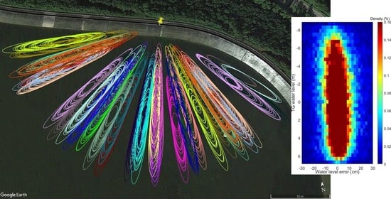
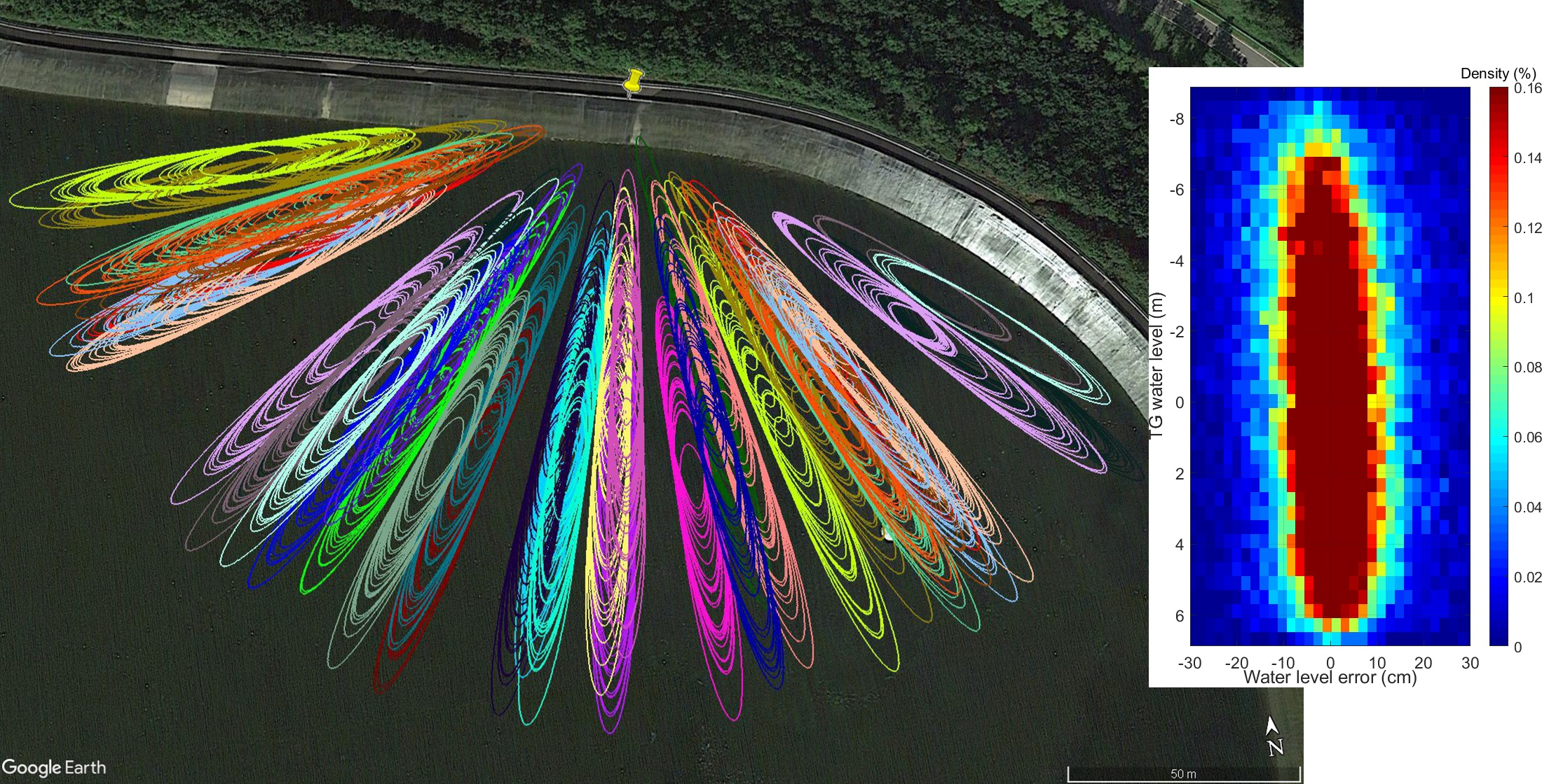
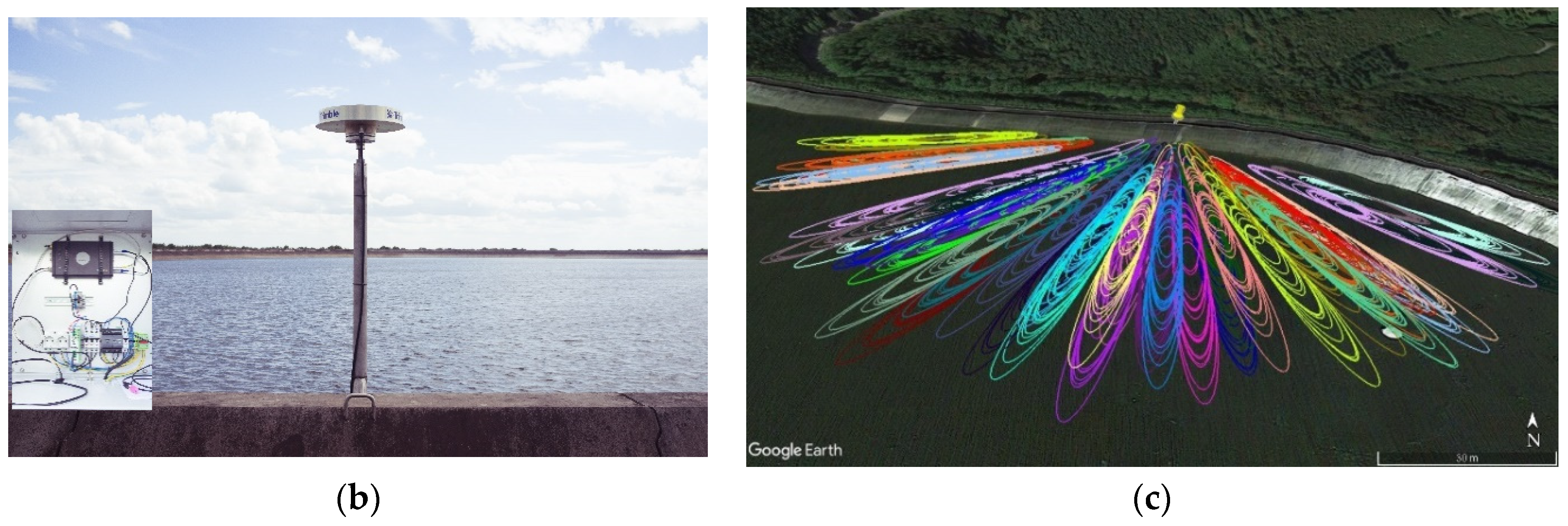
The GNSS station VPSP (latitude: 49.94°, longitude: 6.18°, altitude: 561.96 m) was installed in late-June 2017 at VPSP. It was equipped with a Septentrio PolaRx5 receiver and a Trimble TRM59800.00 antenna with no external radome (Figure 1b). The antenna is installed ~11.0 m above the mean water level, and the receiver was set at a 1-Hz sampling rate. As the station VPSP was installed specifically for GNSS-R, it is positioned towards the south direction in order to maximize the number of satellite tracks (Figure 1c).
VPSP is also equipped with Rittmeyer high-precision pressure gauge MPW2Q sensors. MPW2Q provides hydrostatic or pneumatic pressure measurements every 1 min. MPW2Q reports high-precision water levels (WL) with a resolution better than 1 mm [21].
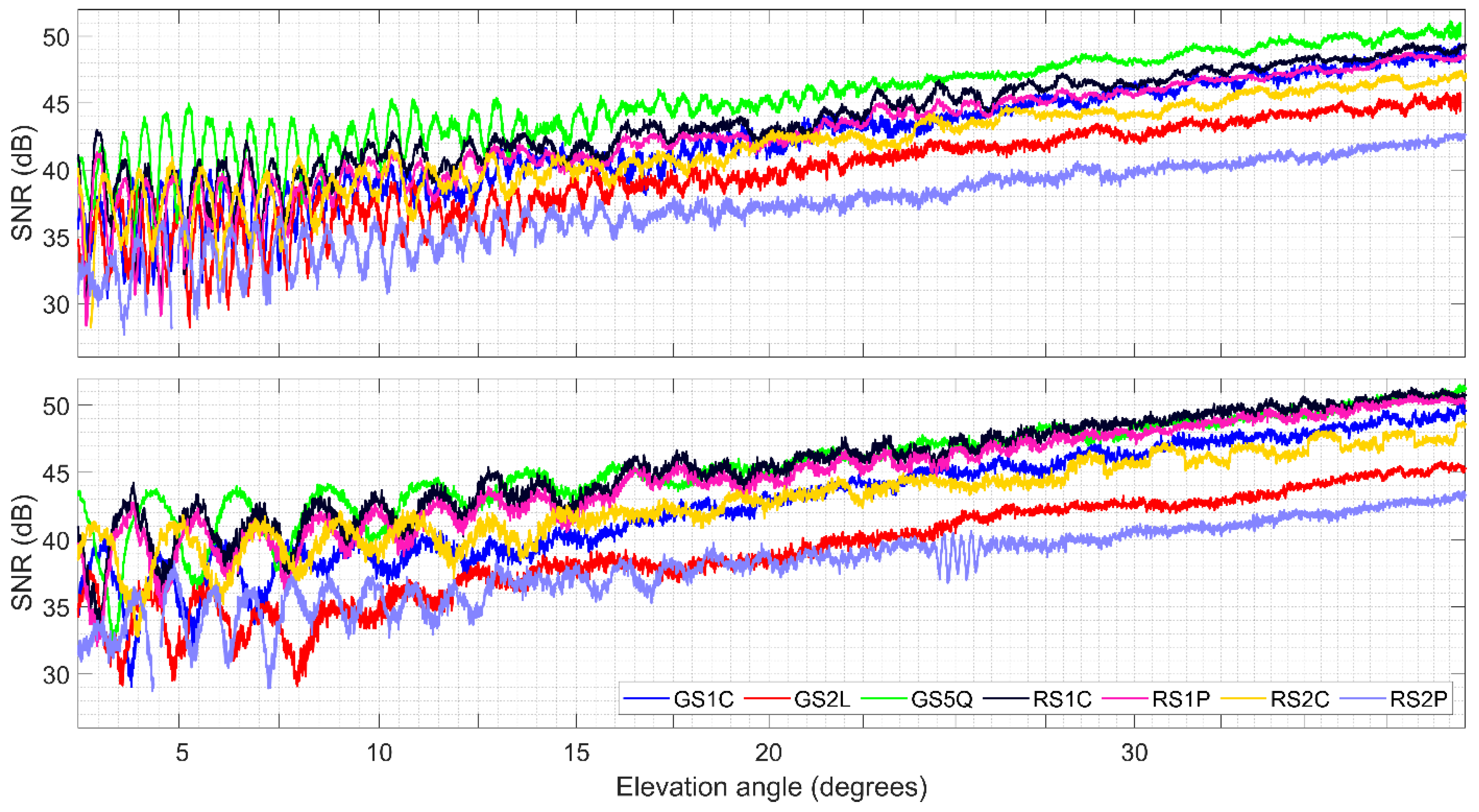
An example of SNR observations of a rising arc at VPSP station is shown in Figure 2. The protected/encrypted signals (P(Y)) on both the L1 and L2 bands are ignored, as they produce nosier SNR fringes [12]. It can be seen that SNR fringes are very clear for all the seven signals, especially for low-elevation angle observations, i.e., observations below a 20° elevation angle. Second, GS5Q have the highest direct power, as no military signal is planned for L5 [11]. Third, there are up to 10-dB different direct power levels between the strongest (GS5Q) and the weakest (RS2P) signals.
3. GNSS-R Data Processing
SNR observations can be decomposed into a trend that is a monotonically increasing function of the elevation angle and detrended interference fringes . The detrended interference fringes that are superimposed on the trend can be expressed in terms of the detrended interference fringes’ amplitude and reflection excess phase with respect to the direct phase [22]:
The interferometric phase is a function of the coupled surface-antenna properties , geometric interference component , and right-handed circularly polarized (RHCP) antenna phase pattern evaluated in the direct path () [23]:
The compositional component of the interferometric phase can be expressed as a function of the complex-valued Fresnel reflection coefficients for same- and cross-sense circular polarization and antenna complex vector effective length () [11,22]:
The geometric component of the interferometric phase can be modeled as a function of the wavenumber ():
Assuming a flat and smooth surface, the interferometric propagation delay () can be modeled as a function of the satellite elevation angle and an a priori reflector height ()—the vertical distance between the GNSS antenna phase center and the reflecting surface [11]:
As the GNSS antenna surroundings (i.e., water level) are an unknown condition, the GNSS-R inverse model is parameterized by a few biases assuming a priori values for the physical parameters. Therefore, the and in the electromagnetic forward model are defined as and , respectively. The real-valued noise power and complex-valued interferometric bias with magnitude and phase are introduced for the interferometric model as [12]:
where the superscript in parentheses is an index; otherwise, it is a power exponent. While the direct and interferometric power biases are introduced only to improve the sinusoid fit to the SNR observations, the interferometric phase bias is used to retrieve the reflector height.
The inverse model can use the forward model internally to simulate SNR observations to estimate parameter corrections by fixing them to their a priori values and corresponding covariance matrices. For more details, the reader is referred to [12] and [23]. Therefore, the interferometric phase can be updated in the forward model as:
Finally, the linear phase bias can be used to estimate the total reflector height:
where is the carrier wavelength.
After inversion, a number of post-processing measures are applied to detect and reject outliers resulting from unexpected situations (i.e., secondary reflections, diminished interferometric powers) of each individual GNSS signal. However, SNR observations should be first clustered so retrieved biases will be compared under comparable environmental conditions. To do that, SNR observations are partitioned into satellite tracks, between rising/setting near the horizon, and culmination near the zenith. The satellite tracks are then clustered by taking advantage of GNSS ground tracks repeatability. Therefore, satellite tracks are discriminated by whether the satellite is ascending or descending near the same azimuth. Intra-signal and intra-cluster quality control (QC) compare the estimated linear phase biases within each individual cluster using robust estimators and statistical intervals and reject outliers resulting from anomalous conditions [9]. In the next step, as phase biases are highly correlated to one another, the constrained least-squares (LS) adjustment is implemented to retrieve constrained constant phase biases to improve the precision of the water level estimates [6].
The water level at VPSP abruptly changes with time. Therefore, the estimated water levels must be corrected for the dynamic water surface level [16]. The interferometric phase rate can be defined as a function of the stationary surface height and height rate correction :
where is the vertical wavenumber [6]. The vertical velocity of the water surface level is an important correction, as the water level at VPSP varies up to 17 m every 4–8 h. Therefore, the height-rate correction can be modeled as:
The first term on the right-hand side represents the angular delay rate, and the second is the integrated delay rate. The height rate and velocity rate can be solved iteratively using the centered finite differences [6]. The elevation angel rate () is derived from the GNSS precise ephemerides. The authors of [6] reported a height rate and velocity rate of about 40 cm/h and 20 cm/h2, respectively, for a GNSS station with about 3-m daily tidal envelopes. Therefore, the height-rate correction cannot be neglected especially at VPSP; otherwise, GNSS-R water levels would be biased. It should be noted that vertical acceleration would be also beneficial, especially when sub-hourly water levels (10 min) with such a window width (2 h) are reported [6].
Tropospheric delays as a function of the satellite elevation angle and the reflector height were found as an important source of error in GNSS-R studies [19,24]. Therefore, here, the estimated water levels are corrected for atmospheric refraction after intra-signal and intra-cluster QC. The Vienna Mapping Function 3 (VMF3) that is based on the ray-traced delays of the ray-tracer RADIATE, together with the Global Pressure and Temperature 3 model (GPT3) on a global grid that represents a comprehensive troposphere model [25], is used to estimate the tropospheric delay corrections. Using the minimum and maximum elevation angle observations of each individual satellite track, the along-path tropospheric delays can be estimated as:
where is the index of refraction along the instantaneous excess delay path [19,24].
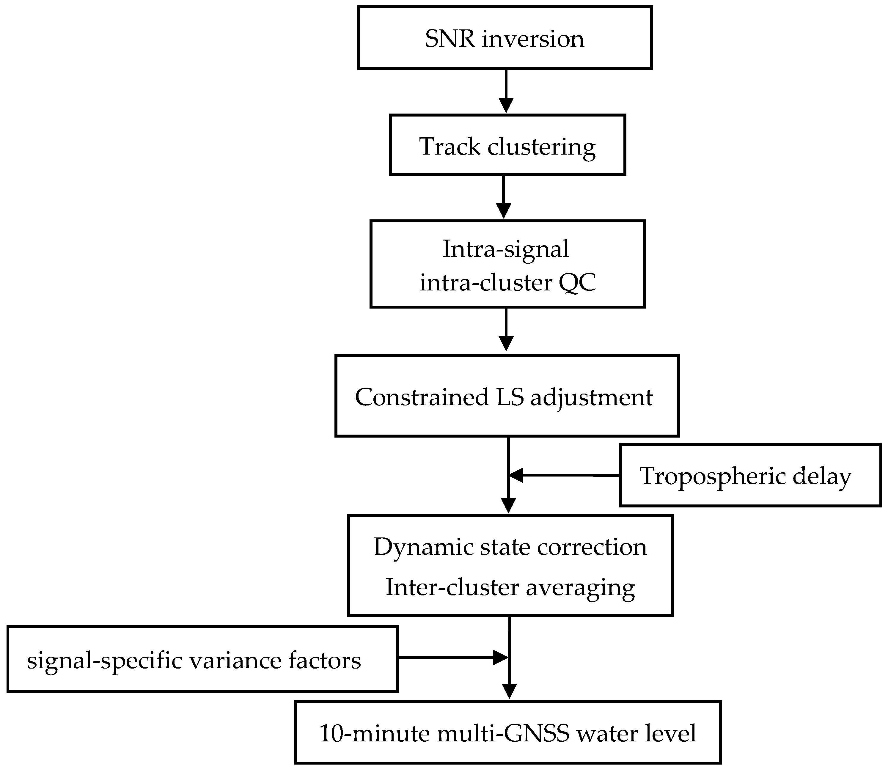
All cluster-by-cluster tracks are combined to produce a regularly spaced signal-specific epoch-by-epoch water level time series together with their respective uncertainties based on a weighted moving average. The moving average returns water levels every 10 min using a 2-h window width [6]. It should be noted that the moving regression is not a simple moving average, as it also estimates the height and velocity rates. Finally, sub-hourly water level time series are reported using the signal-specific variance factors. The statistical inter-signal combination that offers a single multi-GNSS time series was found to improve the precision of geodetic GNSS-R retrievals [12]. The post-inversion algorithm of the water level retrieval at VPSP is summarized in Figure 3.
Before we combined all the independent GNSS-R water levels to provide a single multi-GNSS water level time series, first we compared all the signal-dependent water levels together. Here, the GS1C water level time series is used to evaluate the inter-signal consistency among all the GNSS-R retrievals. A systematic error at a decimeter level between the GPS-L1 and GPS-L2 signal water-surface level retrievals was reported in [26]. In this study, we found linear relationships between different GNSS-R water level estimates and GS1C, with correlations that exceeded 0.98 (Figure 4).
4. Results
Figure 5 shows the tropospheric delays at station VPSP. Due to the variations of the water-surface level, the atmospheric delay changes with respect to the satellite elevation angle. The tropospheric delay difference between the two modes of VPSP when the water-surface level is at its minimum and its maximum is 29.40 cm. The regression slope 0.984 m/m ± 0.001 m/m between the GNSS-R water level time series and WL records are statistically significant vis-à-vis its 95% confidence interval if the tropospheric delay corrections are neglected.
SNR observations from a GNSS station in Sweden, [17] demonstrated that GS2W and RS2P should be avoided for GNSS-R water level studies. The authors of [12] found that legacy GPS signals are worse in terms of accuracy, while modernized GPS and GLONASS signals are comparable. Therefore, signal-specific variance factors are used to report multi-GNSS GNSS-R time series, together with their formal errors (Figure 6).
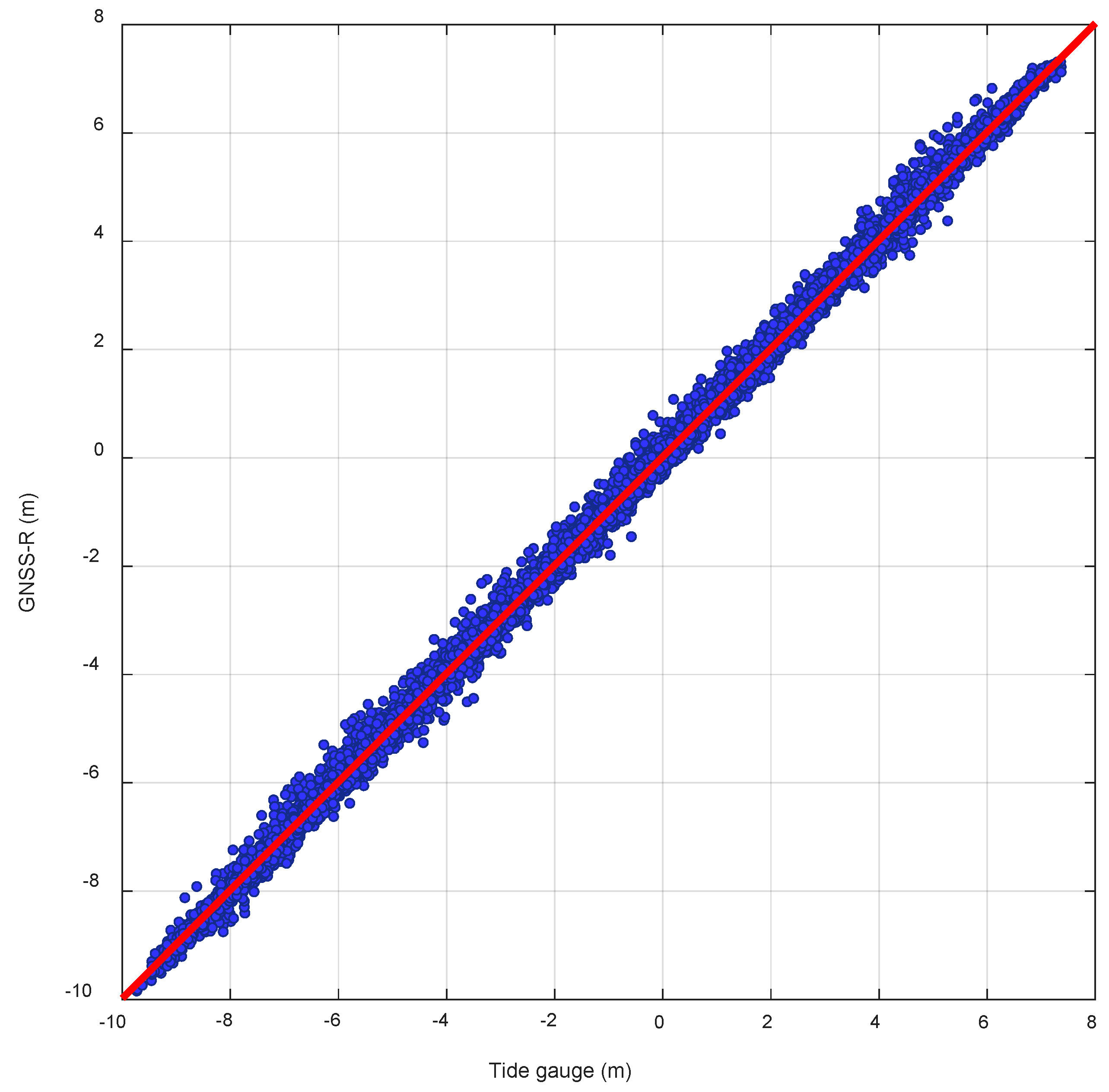
The GNSS-R water level time series are compared with those of the WL records. First, the WL records are interpolated at the GNSS sampling epochs and vice versa by disabling the interpolations across the data outage periods. The RMSE error between the sub-hourly GNSS-R time series and WL records is 7.0 cm. The agreement between the WL records and GNSS-R water level retrievals is excellent, with a correlation coefficient that exceeds 0.999 (Figure 7).
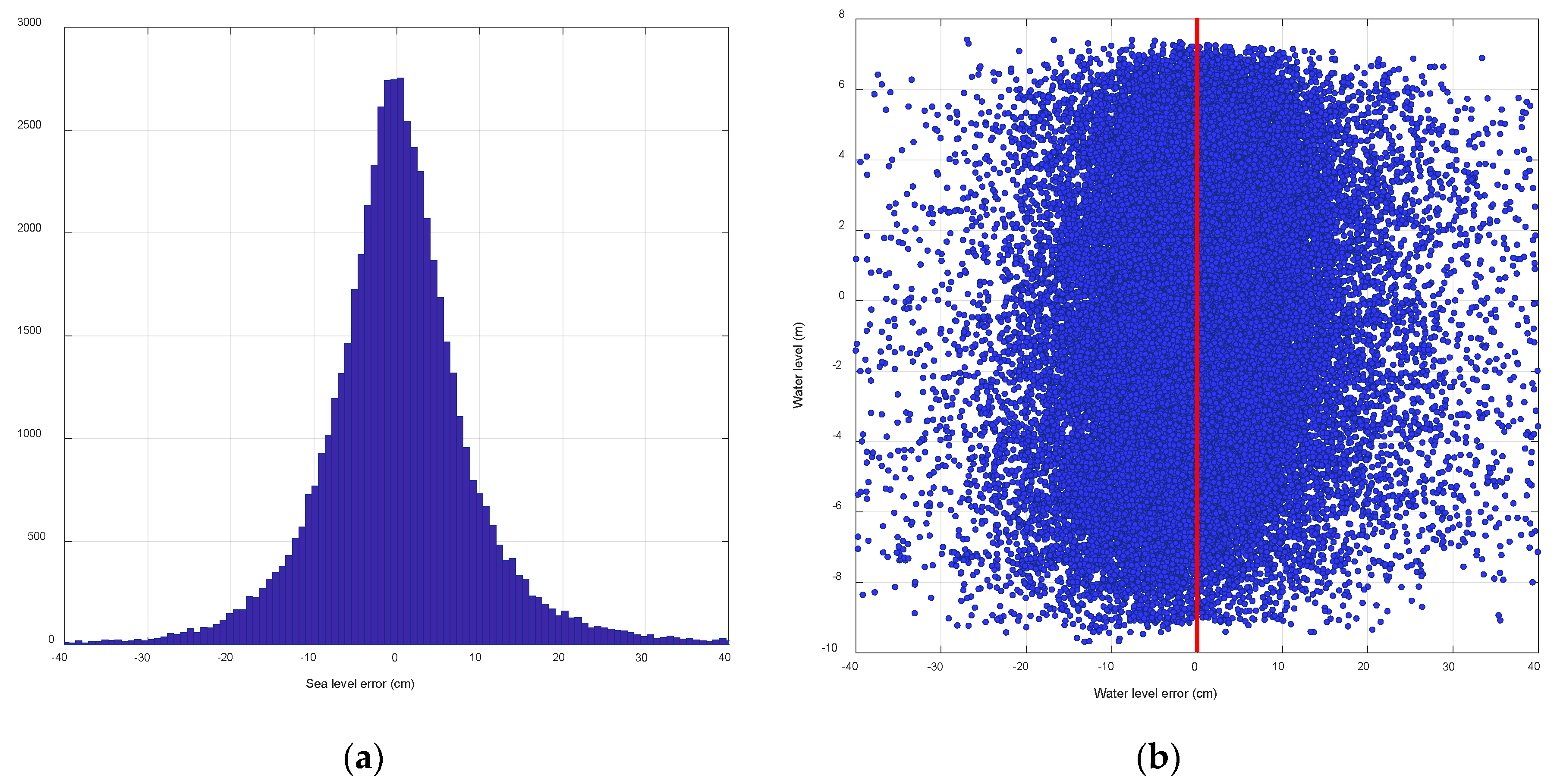
There is no scale error between the GNSS-R water level time series and WL records that can be seen in the van de Casteele diagram in Figure 8. The x-axis presents the difference between geodetic GNSS-R water levels as the test sensor, and the y-axis represents the WL records as the reference sensor. The two water levels deviate by −0.27% from a one-to one relationship. The authors of [4] reported a scale error of 0.84% for a GNSS site with ~2.5-m tidal amplitudes. We found that the RMS reduction at VPSP is 49% when the vertical acceleration is applied. In addition, the GNSS-R water level time series would be deviated by 1.97% from the WL records if they were only corrected for the height rate.
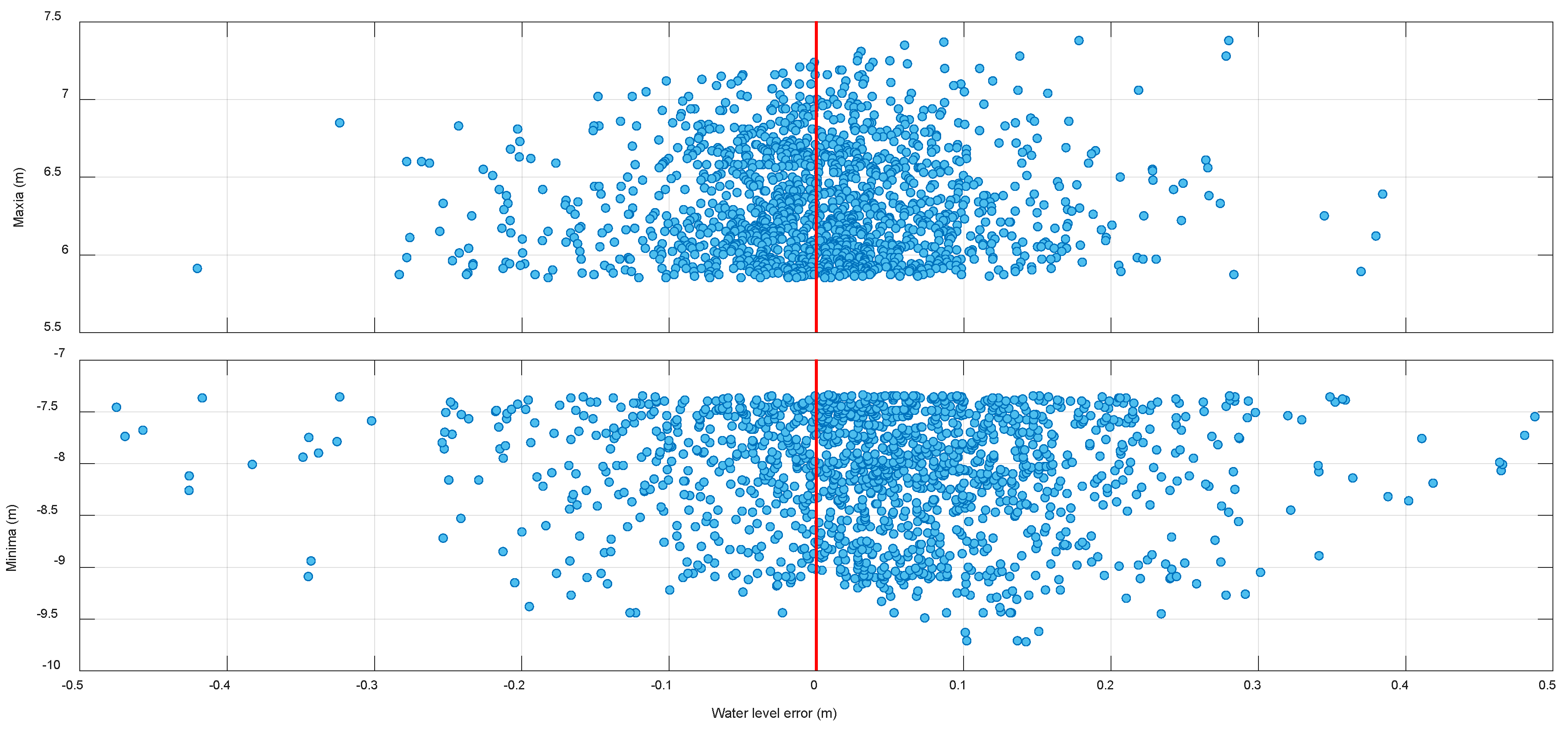
We also compared the sub-hourly maximum and minimum GNSS-R water level retrievals and water level gauge records (Figure 9). The RMSE between the maximum GNSS-R retrievals and water level records is 6.5 cm, but it is 11.1 cm between the minimum GNSS-R estimates and water level measurements.
Carrying out a regression between maxima measurements from the two sensors, the intercept −0.03 m ± 0.16 m and regression slope 0.99 m/m ± 0.03 m/m are not statistically significant vis-à-vis their 95% confidence intervals. The regression intercept of the minima GNSS-R retrievals and water level records is −0.02 m ± 0.19 m, and the regression slope is 1.01 m/m ± 0.02 m/m. While the median offset between the maximum measurements is 0.5 cm, it is 4.7 cm for the minimum retrievals. On one hand, GNSS-R retrievals are less precise than those of the water level. On the other hand, the resolution of the Rittmeyer high-precision pressure gauge sensor is 10 times higher than the GNSS-R, and GNSS-R retrievals are averaged over the FFZs over 10 min. In addition, the offset error between minimum retrievals can be the result of the ramp slope of the dam. When electricity is generated, the water level goes down. Therefore, the vertical and horizonal distances between the GNSS antenna and water surface increase. There would be reflections from the ramp slope for higher elevation angle observations where FFZs are close to the antenna.
5. Conclusions
The geodetic GNSS-R is used to estimate water levels at the Vianden pumped storage plant (VPSP), where the water-surface level changes vertically ~17 m several times a day to generate a peak current. The retrieved heights are corrected for tropospheric delay using VMF3/GPT3 models before signal-specific water levels are estimated based on a weighted moving average using a 10-min post-spacing and a 2-h averaging window width. The inter-cluster combination is implemented in a way to take the dynamic state of the sea surface into account by correcting the retrieved heights for the velocity and vertical velocity corrections. Finally, GNSS-R sub-hourly time series are reported using the signal-specific variance factors. The standard deviation between the sub-hourly GNSS-R water levels and co-located tide gauge records for about one year at the VPSP is 7.0 cm, with a correlation coefficient exceeding 0.999.
The results confirm that GNSS-R can detect sudden and large water surface changes. Therefore, geodetic GNSS-R can be used to study water-surface changes caused by nonastronomical forces such as hurricanes or storm surges. The performance of GNSS-R water levels can be improved in terms of temporal sampling by tracking all GNSS signals from other global navigation systems (i.e., Russian GLONASS, European Galileo, and the Chinese BeiDou global). In the future, the atmospheric bias in he -R water levels will be solved using an atmospheric ray-tracing procedure [24].
Author Contributions
Conceptualization, S.T. and O.F.; methodology, S.T.; software, S.T.; validation, S.T. and O.F.; formal analysis, S.T.; investigation, S.T.; resources, S.T. and O.F.; data curation, S.T and O.F.; writing—original draft preparation, S.T.; writing—review and editing, S.T. and O.F.; visualization, S.T.; project administration, O.F. All authors have read and agreed to the published version of the manuscript.
Funding
This research was carried out at the Geophysics Laboratory of the University of Luxembourg, and received no external funding.
Acknowledgments
The authors would like to thank Société Electrique de l’Our (SEO) for their support in the execution of the VPSP field experiment. We thank F.G. Nievinski for the valuable discussions. We would like to thank Gilbert Klein and Marc Seil for the technical support of the project.
Conflicts of Interest
The authors declare no conflict of interest.
References
- Jin, S.; Cardellach, E.; Xie, F. GNSS Remote Sensing: Theory, Methods and Applications; Remote Sensing and Digital Image Processing; Springer: Dordrecht, The Netherlands, 2014; ISBN 978-94-007-7481-0. [Google Scholar]
- Anderson, K.D. Determination of Water Level and Tides Using Interferometric Observations of GPS Signals. J. Atmos. Ocean. Technol. 2000, 17, 1118–1127. [Google Scholar] [CrossRef]
- Geremia-Nievinski, F.; Makrakis, M.; Tabibi, S. Inventory of published GNSS-R stations, with focus on ocean as target and SNR as observable. Zenodo 2020. [Google Scholar] [CrossRef]
- Larson, K.M.; Ray, R.D.; Williams, S.D.P. A 10-Year Comparison of Water Levels Measured with a Geodetic GPS Receiver versus a Conventional Tide Gauge. J. Atmos. Ocean. Technol. 2016, 34, 295–307. [Google Scholar] [CrossRef] [Green Version]
- Strandberg, J.; Hobiger, T.; Haas, R. Improving GNSS-R sea level determination through inverse modeling of SNR data. Radio Sci. 2016, 51, 1286–1296. [Google Scholar] [CrossRef] [Green Version]
- Tabibi, S.; Geremia-Nievinski, F.; Francis, O.; van Dam, T. Tidal analysis of GNSS reflectometry applied for coastal sea level sensing in Antarctica and Greenland. Remote Sens. Environ. 2020, 248, 111959. [Google Scholar] [CrossRef]
- Geremia-Nievinski, F.; Hobiger, T.; Haas, R.; Liu, W.; Strandberg, J.; Tabibi, S.; Vey, S.; Wickert, J.; Williams, S. SNR-based GNSS reflectometry for coastal sea-level altimetry: Results from the first IAG inter-comparison campaign. J. Geod. 2020, 94, 70. [Google Scholar] [CrossRef]
- Larson, K.M. GPS interferometric reflectometry: Applications to surface soil moisture, snow depth, and vegetation water content in the western United States. Wires Water 2016, 3, 775–787. [Google Scholar] [CrossRef]
- Nievinski, F.G.; Larson, K.M. Inverse Modeling of GPS Multipath for Snow Depth Estimation—Part II: Application and Validation. IEEE Trans. Geosci. Remote Sens. 2014, 52, 6564–6573. [Google Scholar] [CrossRef]
- Small, E.E.; Larson, K.M.; Chew, C.C.; Dong, J.; Ochsner, T.E. Validation of GPS-IR Soil Moisture Retrievals: Comparison of Different Algorithms to Remove Vegetation Effects. IEEE J. Sel. Top. Appl. Earth Obs. Remote Sens. 2016, 9, 4759–4770. [Google Scholar] [CrossRef]
- Tabibi, S.; Nievinski, F.G.; van Dam, T.; Monico, J.F.G. Assessment of modernized GPS L5 SNR for ground-based multipath reflectometry applications. Adv. Space Res. 2015, 55, 1104–1116. [Google Scholar] [CrossRef] [Green Version]
- Tabibi, S.; Nievinski, F.G.; van Dam, T. Statistical Comparison and Combination of GPS, GLONASS, and Multi-GNSS Multipath Reflectometry Applied to Snow Depth Retrieval. IEEE Trans. Geosci. Remote Sens. 2017, 55, 3773–3785. [Google Scholar] [CrossRef]
- Wöppelmann, G.; Marcos, M. Vertical land motion as a key to understanding sea level change and variability. Rev. Geophys. 2016, 54, 64–92. [Google Scholar] [CrossRef] [Green Version]
- Soulat, F.; Caparrini, M.; Germain, O.; Lopez-Dekker, P.; Taani, M.; Ruffini, G. Sea state monitoring using coastal GNSS-R. Geophys. Res. Lett. 2004, 31. [Google Scholar] [CrossRef] [Green Version]
- Löfgren, J.S.; Haas, R.; Scherneck, H.-G.; Bos, M.S. Three months of local sea level derived from reflected GNSS signals. Radio Sci. 2011, 46. [Google Scholar] [CrossRef]
- Larson, K.M.; Ray, R.D.; Nievinski, F.G.; Freymueller, J.T. The Accidental Tide Gauge: A GPS Reflection Case Study From Kachemak Bay, Alaska. IEEE Geosci. Remote Sens. Lett. 2013, 10, 1200–1204. [Google Scholar] [CrossRef] [Green Version]
- Löfgren, J.S.; Haas, R. Sea level measurements using multi-frequency GPS and GLONASS observations. EURASIP J. Adv. Signal Process. 2014, 2014, 50. [Google Scholar] [CrossRef] [Green Version]
- Roussel, N.; Ramillien, G.; Frappart, F.; Darrozes, J.; Gay, A.; Biancale, R.; Striebig, N.; Hanquiez, V.; Bertin, X.; Allain, D. Sea level monitoring and sea state estimate using a single geodetic receiver. Remote Sens. Environ. 2015, 171, 261–277. [Google Scholar] [CrossRef]
- Williams, S.D.P.; Nievinski, F.G. Tropospheric delays in ground-based GNSS multipath reflectometry—Experimental evidence from coastal sites. J. Geophys. Res. Solid Earth 2017, 122, 2310–2327. [Google Scholar] [CrossRef] [Green Version]
- Société Electrique de l’Our. Available online: http://www.seo.lu/ (accessed on 25 May 2020).
- Rittmeyer, A.G. MPW2Q High-Precision Pressure Gauge. Available online: https://rittmeyer.com/en/instrumentation/applications/overview/ (accessed on 24 June 2020).
- Nievinski, F.G.; Larson, K.M. Forward Modeling of GPS Multipath for Near-surface Reflectometry and Positioning Applications. GPS Solut. 2014, 18, 309–322. [Google Scholar] [CrossRef]
- Nievinski, F.G.; Larson, K.M. Inverse Modeling of GPS Multipath for Snow Depth Estimation—Part I: Formulation and Simulations. IEEE Trans. Geosci. Remote Sens. 2014, 52, 6555–6563. [Google Scholar] [CrossRef]
- Nikolaidou, T.; Santos, M.C.; Williams, S.D.P.; Geremia-Nievinski, F. Raytracing atmospheric delays in ground-based GNSS reflectometry. J. Geod. 2020, 94, 68. [Google Scholar] [CrossRef]
- Landskron, D.; Böhm, J. VMF3/GPT3: Refined discrete and empirical troposphere mapping functions. J Geod 2018, 92, 349–360. [Google Scholar] [CrossRef]
- Santamaría-Gómez, A.; Watson, C.; Gravelle, M.; King, M.; Wöppelmann, G. Levelling co-located GNSS and tide gauge stations using GNSS reflectometry. J. Geod. 2015, 89, 241–258. [Google Scholar] [CrossRef]
Figure 1.
Vianden-pumped storage plant (a) (courtesy of the SEO, [20]), global navigation satellite system (GNSS) station VPSP at the Vianden pumped storage plant (b), and (c) occurrences of GS1C first Fresnel zones (FFZs) of July 2018 at the VPSP. Each color depicts each GPS satellite, and the location of the GNSS station is shown as a yellow pin.


Figure 2.
Signal-to-noise ratio (SNR) observations for a rising arc at VPSP for two different epochs when the reservoir had different water levels. Top panel is for decimal year 2018.0024 when the energy demand increased, and bottom panel shows SNR observations for decimal year 2018.0034 when the power consumption was low.

Figure 3.
Flowchart of the water-surface level retrieval algorithm. QC: quality control.

Figure 4.
Scatterplots of the GNSS-derived water level show an excellent agreement between GS1C retrieval and other GNSS-derived water level retrievals; the 1:1 diagonal is shown as a black line.
Figure 4.
Scatterplots of the GNSS-derived water level show an excellent agreement between GS1C retrieval and other GNSS-derived water level retrievals; the 1:1 diagonal is shown as a black line.

Figure 5.
Tropospheric delays at station VPSP.

Figure 6.
Water level time series from Rittmeyer high-precision pressure gauge sensor (red) and geodetic GNSS-R (blue) at the Vianden pumped storage plant (a) and zoom in of the first 15 days of 2018 (b).
Figure 6.
Water level time series from Rittmeyer high-precision pressure gauge sensor (red) and geodetic GNSS-R (blue) at the Vianden pumped storage plant (a) and zoom in of the first 15 days of 2018 (b).

Figure 7.
Scatterplot of the water levels show an excellent agreement between GNSS-R retrievals and water level (WL) records.
Figure 7.
Scatterplot of the water levels show an excellent agreement between GNSS-R retrievals and water level (WL) records.

Figure 8.
Histogram of the water level error between the GNSS-R and WL sensor at the VPSP (a), and van de Casteele diagrams for the GNSS-R water levels over 1 year at the VPSP (b).
Figure 8.
Histogram of the water level error between the GNSS-R and WL sensor at the VPSP (a), and van de Casteele diagrams for the GNSS-R water levels over 1 year at the VPSP (b).

Figure 9.
Van de Casteele diagrams for the sub-hourly water level extremes measured by the GNSS-R and water level gauge.
Figure 9.
Van de Casteele diagrams for the sub-hourly water level extremes measured by the GNSS-R and water level gauge.

Publisher’s Note: MDPI stays neutral with regard to jurisdictional claims in published maps and institutional affiliations. |
© 2020 by the authors. Licensee MDPI, Basel, Switzerland. This article is an open access article distributed under the terms and conditions of the Creative Commons Attribution (CC BY) license (http://creativecommons.org/licenses/by/4.0/).
Share and Cite
MDPI and ACS Style
Tabibi, S.; Francis, O. Can GNSS-R Detect Abrupt Water Level Changes? Remote Sens. 2020, 12, 3614. https://doi.org/10.3390/rs12213614
AMA Style
Tabibi S, Francis O. Can GNSS-R Detect Abrupt Water Level Changes? Remote Sensing. 2020; 12(21):3614. https://doi.org/10.3390/rs12213614
Chicago/Turabian StyleTabibi, Sajad, and Olivier Francis. 2020. "Can GNSS-R Detect Abrupt Water Level Changes?" Remote Sensing 12, no. 21: 3614. https://doi.org/10.3390/rs12213614
Note that from the first issue of 2016, this journal uses article numbers instead of page numbers. See further details here.