Estimation of the Number of Endmembers in Hyperspectral Images Using Agglomerative Clustering


Instituto de Telecomunicaciones y Aplicaciones Multimedia, Universitat Politècnica de València, 46022 Valencia, Spain
*
Author to whom correspondence should be addressed.
Remote Sens. 2020, 12(21), 3585; https://doi.org/10.3390/rs12213585
Submission received: 21 September 2020
/
Revised: 23 October 2020
/
Accepted: 29 October 2020
/
Published: 1 November 2020
(This article belongs to the Special Issue New Advances on Sub-pixel Processing: Unmixing and Mapping Methods)
Abstract
:Many tasks in hyperspectral imaging, such as spectral unmixing and sub-pixel matching, require knowing how many substances or materials are present in the scene captured by a hyperspectral image. In this paper, we present an algorithm that estimates the number of materials in the scene using agglomerative clustering. The algorithm is based on the assumption that a valid clustering of the image has one cluster for each different material. After reducing the dimensionality of the hyperspectral image, the proposed method obtains an initial clustering using K-means. In this stage, cluster densities are estimated using Independent Component Analysis. Based on the K-means result, a model-based agglomerative clustering is performed, which provides a hierarchy of clusterings. Finally, a validation algorithm selects a clustering of the hierarchy; the number of clusters it contains is the estimated number of materials. Besides estimating the number of endmembers, the proposed method can approximately obtain the endmember (or spectrum) of each material by computing the centroid of its corresponding cluster. We have tested the proposed method using several hyperspectral images. The results show that the proposed method obtains approximately the number of materials that these images contain.
1. Introduction
Some tasks in hyperspectral imaging, such as classification and unmixing, require knowing how many pure substances or materials are present in a scene [1]. In recent years, some algorithms have been proposed to estimate the number of materials in a hyperspectral image [2,3,4,5,6,7,8]. Although these algorithms are based on different principles, most of them work by analyzing the eigenvalues of the covariance matrix of the image. In this paper, we present a novel method that departs from previous works and that uses agglomerative clustering.
The information captured by a hyperspectral sensor with N cells and L spectral bands can be represented by an matrix, , where each column of is a pixel of the image. The l-th component of a pixel is the radiance measured by the cell of that pixel at the l-th spectral band (). Hence, each pixel can be thought of as an L-band spectrum. Since L is usually larger than 100, the processing of hyperspectral images is computationally complex. The scene captured by a hyperspectral sensor contains a set of materials. Generally, the number of materials, K, is much smaller than the number of bands of the hyperspectral sensor (i.e., ). Each material in a scene has a representative L-band spectrum, called endmember.
Many algorithms infer the number of materials in a scene by determining the number of different endmembers that are present in a hyperspectral image of that scene. In most of these algorithms, the estimation of K is based on the eigenvalues of the correlation matrix of [3,4,5,6,7,9].
In this paper, we present a new approach that estimates the number of endmembers of a hyperspectral image using clustering techniques. The proposed method first generates a set of partitions of using clustering, and then it selects the optimal partition according to a certain validation index. We assume that each cluster of the optimal partition corresponds to a different endmember, and, consequently, the proposed method sets the estimated K to the number of clusters of that partition. Our clustering algorithm is a model-based two-stage agglomerative technique. The use of a model-based clustering allows us to overcome some problems that arise in conventional clustering approaches. Cluster densities are modeled using Independent Component Analysis (ICA). The two-stage clustering consists of a partitional clustering stage and an agglomerative clustering stage. The partitional stage provides a reduced number of clusters, which facilitates the subsequent and more complex agglomerative stage.
The contributions of this paper can be summarized as follows. First, we propose a new approach to the estimation of the number of endmembers which is based on clustering principles (in contrast to most existing algorithms which are based on the eigenvalue spectrum of the correlation matrix). Second, we propose a specific model-based two-stage agglomerative algorithm to perform the clustering. The proposed model is Independent Component Analysis, a general model which can pretty fit to non-Gaussian and correlated scenarios. In contrast to other methods, our algorithm also allows to approximately obtain the endmembers of the constituent materials and a segmentation of the hyperspectral image.
Background and Related Work
Devising an algorithm to estimate the number of endmembers requires assuming a certain model for the generation of the hyperspectral image. The most commonly used model is the linear mixing model (LMM) [2]. In this model, each pixel is a random vector of the form
where is the set of endmembers; coefficients , called abundances, are random variables that represent the fraction of each endmember in ; and the noise term, , is a random vector that accounts for any model or measurement error. In LMM, random vectors and are independent. Moreover, abundances satisfy () and , which are called the abundance constraints. Under the LMM, a hyperspectral image matrix can be written as
where is the signal component of , is the noise component of , is a matrix whose columns are the endmembers of , and is a matrix whose columns contain the abundances of each pixel of .
Let be the correlation matrix of a random vector that follows the LMM and let be the sequence of eigenvalues of arranged in decreasing order. Suppose that is white, that is, and for some ( stands for the identity matrix). In this case, for , and for . Eigenvalues are due to signal (and noise), while eigenvalues are only due to noise. Since the sequence of eigenvalues has a “knee” at index , we can determine K by identifying this knee.
In practice, identifying the knee in the sequence of eigenvalues is difficult for two reasons. First, since is not available, we must consider the sequence of eigenvalues of the sample correlation matrix , which is an estimation of [2]. Second, the white noise assumption is not valid in hyperspectral images since the components of usually have very different variances and are correlated. As a consequence, the sequence of ordered eigenvalues does not show a clear knee [4]. In the following, we briefly describe several algorithms that try to cope with these problems.
The Harsanyi-Farrand-Chang (HFC) algorithm [3] assumes that the noise is white and Gaussian. This algorithm performs a binary Neyman-Pearson hypothesis test to decide if each is due to signal or due to noise. After performing the L hypothesis tests, HFC sets the estimated number of materials to the number of eigenvalues that has been decided to be due to signal. An issue of HFC is that the user must provide the value of the false-alarm probability used in the hypothesis tests. Moreover, HFC assumes that is white, which is not a proper assumption in hyperspectral images. This last drawback is addressed by a variation of HFC, called Noise Whitened HFC (NWHFC) [5]. NWHFC first estimates the noise variance in each band using the residual method proposed in [10]; then uses the estimated noise variances to whiten the image data, and, finally, applies HFC on the whitened data.
The hyperspectral subspace identification algorithm by minimum error (HySime) tries to identify the linear subspace where the noise-free image lies and sets to the dimension of the identified subspace. HySime first estimates the noise matrix (using an algorithm based on the same principles that the residual method [10]) and computes its sample correlation matrix . Then, it estimates the signal matrix and its sample correlation matrix . Finally, HySime selects that subset of eigenvectors of , , that minimizes the mean squared error between the columns of and their projections over the space spanned by . The number of eigenvectors in is set to .
The so-called RMT algorithm in [6] identifies the eigenvalues of the covariance matrix of that are due to signal using a sequence of hypothesis tests that, unlike HFC and NWHFC, are based on results of random matrix theory (RMT) [11]. The Noise-whitened Eigengap approach (NWEGA) is also based on RMT, but the hypothesis tests are based on the gaps between successive eigenvalues, not on the eigenvalues themselves [7]. As NWHFC and HySime, both RMT and NWGEA need to estimate the noise statistics of the image. RMT assumes that the noise is spectrally uncorrelated (i.e., is diagonal) and estimates the variance of the noise in each band using the algorithm in [12]. NWEGA uses the full covariance matrix of the noise, which is estimated using the same algorithm as in [4]. Other RMT-based algorithms have recently been introduced in [9].
The performance of the algorithms that rely on the image noise statistics depends on how accurately these statistics are estimated [13,14]. The residual method [10] has been widely used since it provides more accurate estimates than other well-known algorithms [13]. An improvement of the residual method, called the modified residual method, is introduced in [15]. In [14], the accuracies of five estimators of the band noise variance are compared, and the results show that the modified residual method is the most accurate. However, the variance estimates of the modified residual method are not guaranteed to be positive. This drawback is fixed in the methods proposed in [14,16].
All of the above algorithms are based on the LMM, which assumes that each material of the scene is represented by a single endmember. In practice, however, the endmember of a material may spatially vary due to changes in the illumination or variations in the intrinsic features of the material, among other causes. To address endmember variability, some alternatives to the LMM have been proposed (e.g., see [17,18,19,20]). One of them is the normal compositional model (NCM), which accounts for endmember variability (and other sources of uncertainty) by using random endmembers [17]. In NCM, each pixel is modeled as the mixture
where the endmembers are independent Gaussian random vectors, and the abundances meet the abundance constraints. An algorithm for estimating the number of endmembers that is based on the NMC is presented in [8]. This algorithm assumes that the components of each are independent, that the mean of each belongs to a known spectral library, and that the covariance matrix of each is of the form . The algorithm assumes a Bayesian model whose parameters are the mean vectors, the variance , the number of endmembers K, and the abundances. The estimation of parameters, and hence K, is performed using a Reversible-Jump Monte Carlo Markov Chain method.
The rest of the paper is organized as follows. In Section 2, we justify the use of clustering to estimate the number of endmembers in hyperspectral images. In Section 3, we present a detailed description of the proposed algorithm. In Section 4, we experimentally assess the performance of the proposed method on four hyperspectral images. The results obtained are discussed in Section 5. Finally, Section 6 summarizes the main points of the paper and comments on future work.
2. Estimation Using Model-Based Agglomerative Clustering
We have seen that existing methods for the estimation of the number of endmembers rely on determining the dimension of the signal subspace. This is mostly made by determining the number of signal eigenvalues. However this approach might be problematic in a practical setting. Thus, in a real image, many of the N pixels may have a predominant endmember, i.e., one of the abundances () is close to 1 while the rest are negligible. Moreover, in the whole image some endmembers can be much more numerous than others. Let us make some analysis about the implications of these two practical conditions. We will resort to LMM, hence let us compute the data autocorrelation matrix. Assuming that signal and noise vectors are uncorrelated we may write
where the endmember matrix was defined in (1) and we have defined the abundance vector . Notice that in the limiting situation in which every pixel is explained by only one endmember, every particular realization of the random matrix will be a diagonal matrix, with all the main diagonal elements, except one, equal to zero. Actually, the i-th element of the main diagonal will be a binary random variable having a probability of 1 equal to the prior probability of the i-th endmember, . Hence, the mean value of that binary random variable will be , then we can write from (3)
Now, let us call , , () to the eigenvalues of matrices , , and , respectively. Notice in (4) that if a few endmembers are much more abundant than the rest, many inputs in the diagonal matrix will be close to zero and the actual rank of matrix will be much less than K, i.e., many eigenvalues of will be zero. We can say that the most numerous endmembers “hide” the less abundant ones. It is well-known that the eigenvalues of the sum of two Hermitian matrices satisfy the following inequalities
That for reduces to
Therefore, if many eigenvalues of the signal component are zero, the eigenvalue spectrum of is mainly dominated by the eigenvalue spectrum of and this may lead to poor estimation of the true number of endmembers.
We propose in this paper a different approach based on clustering. If every particular endmember is predominant in a given number of pixels, it should be possible to define a cluster centered on it. Notice that the finding of a proper cluster of pixels around a given endmember depends on the absolute number of pixels where that endmember is predominant, but not on the relative number of pixels with respect to other endmembers. In that way, it should be possible to mitigate the hiding phenomenon of the less numerous endmembers.
A clustering algorithm partitions a set of objects into subsets or clusters in such a way that objects that belong to a certain cluster are closer in some sense than objects that belong to different clusters [21]. There are two main types of clustering: partitional clustering and hierarchical clustering. Partitional clustering provides a single partition of the objects, whereas hierarchical clustering generates a sequence of nested partitions or partition hierarchy. There are two major hierarchical clustering algorithms: agglomerative algorithms and divisive algorithms. Agglomerative algorithms start with each object being its own cluster and successively merge pairs of clusters until there is only one left. In contrast, divisive algorithms start with a single cluster (that represent all the objects) and successively split a cluster into two new clusters (until the number of clusters equals the number of objects).
In partitional clustering, the number of clusters, P, is an input parameter which is generally unknown. To obtain a proper P value, data is clustered with each value of P in a certain range, and the partition with the highest quality is selected. The task of evaluating the quality of a clustering is called cluster validation, and a function that measures the quality of a partition is called a validity index. Hierarchical clustering does not require a value of P as input parameter, but we must decide which is the best partition of the hierarchy. This is also done using a proper validity index. A large number of validity indexes have been proposed for each type of clustering but none has shown good performance in all applications [22].
Conventional clustering methods rely on measuring both intra-cluster and inter-cluster distances (typically the Euclidean distance). This may be considered a nonparametric approach, as not any particular model is assumed for the data distributions. However, parametric (or model-based) approaches could be competitive alternatives if some parametric model can be defined. Thus, conventional distance measures could be replaced by model distance measures. We have seen that LMM is a standard parametric model in the application considered in this work. Inspired by it, we will consider a different linear model suitable for the clustering approach. Specifically we propose the use of the ICA model. In ICA every pixel vector having the i-th predominant endmember is expressed in the form
where is the centroid of the cluster and models the contributions from noise and/or other less predominant endmember. Notice that the elements of vector are independent random variables having arbitrary probability densities, and that the matrix incorporates the correlation among the elements of the random fluctuations around the centroids. It could be said that we have exchanged the two contributions in LMM. Now only one endmember appears instead of the K included in the matrix-vector product of the LMM. On the contrary, the isolated noise term has been replaced by thus allowing to incorporate both correlation and non-Gaussianity. Also notice that a different ICA model is to be estimated for every endmember, in contrast with the global LMM. This allows a more focused searching of every endmember and, in fact, endmember estimates (the centroids , ) are also obtained.
As in [23], the clustering performed by the proposed method is an agglomerative approach. To reduce the computation complexity of the agglomerative clustering, two previous steps are performed. First, dimensionality reduction is applied to the image data using Principal Component Analysis (PCA). The resulting feature vectors are then clustered using a partitional algorithm. The reduced number of clusters provided by the partitionl clustering and the small number of variables of their constituent vectors reduce the computational burden of the subsequent agglomerative clustering.
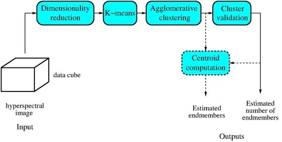
Based on the above, we propose an model-based agglomerative clustering algorithm for determining the number of endmembers in a hypersepectral image. After a preprocessing that transforms each pixel into a feature vector (using PCA), the proposed method generates a hierarchy of partitions for an image by performing a two-stage clustering. First, a partitional clustering is applied to , which provides an initial partition . Then, an agglomerative clustering is performed on , which provides a hierarchy of partitions. The agglomerative clustering algorithm models the probability density of each cluster in using ICA and measures the distance between each pair of clusters using the symmetric Kullback-Leibler (SKL) divergence of their corresponding densities. In each merging step of the agglomerative clustering, the two existing clusters with the smallest SKL divergence are merged. Finally, a cluster validation using a proper index selects the best partition of the hierarchy, and the number of clusters of that partition is set to the estimated K. Figure 1 shows the main steps performed by the proposed algorithm.
The agglomerative clustering performed by the proposed method is similar to the one in [23]. Thus, the algorithm in [23] also models the clusters using ICA, and those clusters that have the minimum SKL divergence are merged. However, the algorithm in [23] assumes that the feature vectors of the image are drawn from an ICA mixture model [24,25], whose ICA parameters are jointly estimated using a maximum likelihood approach. In contrast, the method proposed in this paper models each cluster of using an independent ICA model, which facilitates the estimation of its parameters. Unlike LMM, the combination of multiple ICA models allows non-linearity between variables to be considered, and thus, different local linear relations between variables could be modeled.
3. Materials and Methods
In this section, we describe the proposed method (see Algorithm 1). The algorithm has two inputs: the image data ( matrix) and the maximum number of endmembers to be estimated P. Its output is the estimated number of endmembers . Estimation is performed in four steps: preprocessing, partitional clustering, agglomerative clustering, and cluster validation. In the following, we give a detailed description of each step, explaining its role in the overall process and justifying the techniques used.
| Algorithm 1: Estimation of the number of endmembers using agglomerative clustering. |
| Input: ( matrix of image data), P (maximum number of endmembers) Output: (estimated number of endmembers) 1. Preprocessing. Perform centering, PCA, and normalization: 2. Partitional clustering. Perform K-means with P clusters: 3. Agglomerative clustering. Obtain a hierarchy of partitions: 3.1 Density estimation. Estimate the density of each cluster in using ICA: 3.3.1 Select the two closest clusters of and merge them into a new cluster. Set the remaining clusters to partition . 3.3.2 Compute the distance between the new cluster and the rest of clusters of . 4. Cluster validation. Select a partition of the hierarchy and obtain : . |
3.1. Preprocessing
The preprocessing step transforms the pixels of into feature vectors in order to facilitate the subsequent clustering steps. This preprocessing involves performing a sequence of three tasks: centering, dimensionality reduction, and normalization. Centering provides zero-mean (band) variables. The centered image is obtained with
where is an matrix with all its columns equal to .
Dimensionality reduction is performed by applying (PCA) to the centered image. The number of principal components that are retained, M, is the minimum that explains at least 99% of the total variance of . This step is implemented with
where is an matrix whose columns are the eigenvectors of the correlation matrix of that have the M largest eigenvalues associated to them. Note that the resulting matrix, , is .
Finally, is normalized so each transformed variable (or row of ) have unit variance. Let be the diagonal matrix whose i-th diagonal entry is the inverse of the standard deviation of the i-th row of . Normalization is performed with
3.2. Partitional Clustering
Partitional clustering partitions the N columns of into P clusters using the K-means algorithm. K-means tries to iteratively find the partition that minimizes the cost function
where is the mean of the feature vectors in cluster , and is a distance function for vectors in . The algorithm inputs are , P and an initial set of mean vectors. The resulting partition is represented with P matrices, , where the columns of are those of that have been assigned to . K-means generally converges to a local minimum of the cost J, which depends on the initial set of mean vectors [22]. To obtain a high quality partition, the proposed method runs K-means several times (each with a random set of initial means), and selects the partition of the run having the smallest J. The number of times that K-means is iterated is a trade-off between computational complexity and stability in the resulting partition.
3.3. Agglomerative Clustering
If , the initial partition will be finer than a correct partition (that is, one in which each of its K clusters corresponds to a different material). The agglomerative clustering of generates a hierarchy of partitions, where and has a single cluster with all feature vectors. The hierarchy of partitions is obtained by performing three operations sequentially: density estimation, distance computation, and merging. Each of these operations is described below.
3.3.1. Density Estimation
The agglomerative clustering starts by evaluating the density of each cluster at each of its corresponding feature vectors. To do this, we model the vectors of each cluster using ICA [26]. ICA models a cluster with a random vector of the form
where the mixing matrix () and the bias vector () are deterministic, and the source vector is a zero-mean random vector with independent components. We assume that is invertible, and, therefore, we can write
From this, and taking into account that the components of are independent, the density of cluster can be written as
where denotes the density of the i-th component of .
The ICA parameters of each cluster (columns of ) are obtained in the following way. First, the proposed method sets to the mean of the feature vectors of (i.e., the centroid of ), and subtracts from each column of . Then, it obtains the mixing matrix of the centered cluster using an ICA algorithm. From and , the algorithm obtains the source vector of each feacture vector using (14). Finally, the resulting source vectors are arranged in an source matrix . As is shown below, ICA parameters allows us to measure distances between clusters.
As already indicated, the clustering approach assumes that every pixel has a preponderant endmember. This is modelled in (9) by the centroid . Then, the linear model in (9) accounts for the possible random contributions of other endmembers as well as noise or model errors. Note that this random contribution is quite general. Non-gaussianity is incorporated by the densities of the sources , and statistical dependence is obtained by the transformation matrix . This is in contrast with the other linear models previously mentioned in Section 1.1, which assume Gaussianity and independence or require explicit estimation of the noise correlation matrix. The degrees of freedom of mixtures of ICAs for density estimation allow complex geometry of data with many possible levels of dependence to be modeled [24]. This provides great flexibility to allocate pixel cluster membership during the different levels of iterative process of hierarchical clustering where several ICA-based clusters are fused [25].
3.3.2. Distance Computation
In this step, the distance between any pair of clusters of is computed. We define the distance between two clusters, and , as the SKL divergence between their corresponding cluster densities, which is defined as [27]:
The SKL divergence is commonly used to measure the dissimilarity between two distributions [28,29]. Appendix A describes how is estimated from the mixing matrix, the bias vector and the source matrix of and .
3.4. Cluster Merging
From the SKL distances between the clusters of , the hierarchy is generated using an iterative merging process. In the r-th iteration (), the two closest clusters (in the SKL-distance sense) of partition (with clusters) are merged into a new cluster, and the originating clusters are removed, providing partition (with clusters). Before the r-th merging, the KL distance between each pair of clusters in must be computed. For , these KL distances can be easily computed as is shown below.
Suppose that the -th recursion has generated cluster by merging clusters and . The density of can be written as
where and are the prior probabilities or proportions of and , respectively. The prior probability of the new created cluster is
Taking into account (17), the KL distance between the new created cluster and any other cluster can be expressed as
where since . By using (17)–(19), in each iteration r (), the SKL distance between every pair of clusters in is computed and the two closest clusters are merged (when , only merging is necessary since the distances are already available).
3.5. Clustering Validation
Ideally, one of the partitions in will be close to a correct clustering of the image and the number of clusters in that partition will be the number of endmembers (K). In the final validation step, the proposed method selects one of the clusterings of the hierarchy and sets to the number of clusters that it contains. In agglomerative clustering, validity indexes are often based on the sequence of minimum distances that are obtained in the merging process. Examples of such indexes are the upper tail rule [21,30] and the inconsistency coefficient [31]. These indexes provide a simple validation, but they depend on some input parameters that must be set by the user and whose appropriate values depend on the type of data that is analyzed [21].
The validation performed by the proposed method is based on a sequence, , that is built into the merging process. Specifically, at each iteration r, the proposed method computes the centroid of each of the two clusters in that are merged, say and ; and obtains the value of at with
Hence, is proportional to the euclidean distance between the centroids of the merged clusters in (the partition of the hierarchy that has k clusters). After obtaining sequence (), the estimated number of endmembers is set to
Let us justify the use of the above validity index. Assume that and that there is no error in the merging process, that is, clusters of different endmembers are only merged when . If a cluster essentially contains all pixels of a certain material, then we can expect that the cluster centroid will be close to the endmember of that material in the normalized feature space. At iteration , the computed will be generally small since contains some clusters that belong to a same material and whose means will be therefore close. As r increases, these artificial clusters will merge, and we can expect the minimum distance between cluster to increase until iteration . At this iteration, two clusters representing different materials (i.e., with distant centroids) will be merged and, hence, we can expect a large . When r increases above , the number of materials whose clusters have been merged increases, and we can expect cluster centroids will approach each other ( will decrease as k approaches 2). Summarizing the above, we can expect that sequence will reach its maximum value at an index k close to K.
4. Experimental Results
In this section, we present the results provided by the proposed method (implemented in MATLAB) in the estimation of the number of endmembers of four hyperspectral images (Samson, Jasper Ridge, Urban, and Wasington DC). We also show some partitions provided by our method and their cluster centroids. Finally, we compare the results obtained to those obtained using five well-known algorithms.
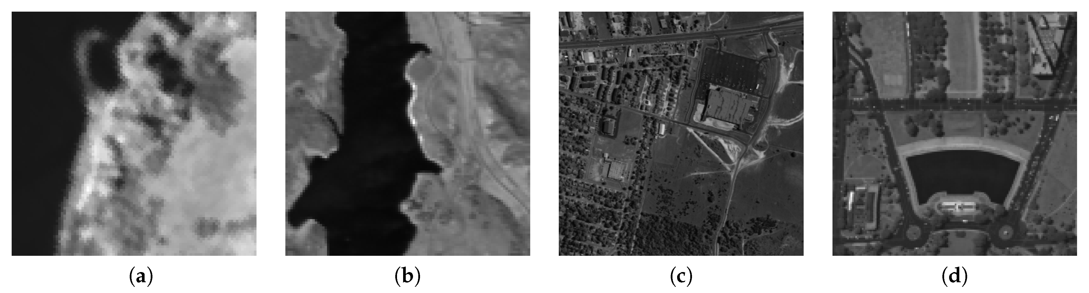
Figure 2 shows the four hyperspectral images that have been used to test the proposed method (the result of averaging the image bands is displayed as a grayscale image). All four images are publicly available and have been widely used to asses the performance of hyperspectral processing algorithms. Ground truth classifications of the test images have been published and their constituent materials have been identified [32]. In all images except Samson, some spectral bands have been removed since they are very noisy.
For each test image, Table 1 shows the spatial dimensions, the number of bands considered in the estimation, and the number of bands of the original image (in parentheses). Samson has three endmembers (Soil, Tree, and Water), and Jasper Ridge has four endmembers (Road, Soil, Water, and Tree). There are several ground truths for the endmembers of Urban: one with four endmembers (Asfalt, Grass, Tree, and Roof) as considered in [33,34,35], one with five endmembers (the previous four plus Soil) [32], and one with six endmembers [34]. The ground truth of Washington DC contains six endmembers (Roof, Grass, Water, Tree, Trail, and Road).
Table 2 shows the values of obtained for each test image after executing our algorithm 25 times with . In each execution, the initial partition is determined by repeating K-means 15 times and then selecting that partition with the minimum cost. To decrease the sensitivity of K-means to data outliers, the city-block distance is used instead of the usual squared Euclidean distance. For each image, the number of times that each value has been obtained is specified in parentheses (nothing is specified when the same value is obtained all 25 times). Table 2 also shows the number of endmembers K (according to some published ground truths) for comparison (three values are shown in Urban since it has three ground truths, as mentioned above). Note in Table 2 that the estimated values are highly stable (most runs provide the same value) and close to K. The accuracy and stability of the estimation decreases when the number of K-means repetitions is decreased. For instance, in Jasper Ridge, in 22 of the 25 runs when K-means is repeated 10 times and in 11 of the 25 runs when K-means is repeated 5 times (in this last case, in 4 runs, in 3 runs, and in 7 runs).
Table 3 shows the estimated number of endmembers provided by using HFC, NWHFC, HySime, RMT, and NWEGA for each test image. For HFC and NWHFC, the values of are shown when the false-alarm probability () is , , and since these are the values used in most papers [4,7,14]. In RMT, the regression-based noise-estimation algorithm of [4] was used instead of the spatial-based algorithm used in [6]. Table 3 also shows the results obtained by using the proposed method (for the images Jasper Ridge and Washington DC, the most frequent is shown). Note that HFC, NWHFC, HySime, RMT, NWEGA overestimate the number of endmembers in these four test images. The estimation error is especially large in the image Urban. In HFC and NWHFC, decreases with decreasing (as expected); however, even with , both methods overestimates K in all four images.
Table 4 shows the running times of the six algorithms on a desktop computer with an Intel Core i7-9700 CPU and 16 GB of RAM (DDR4-2666). HFC is the fastest algorithm since it does not estimate the noise statistics. HySime, RMT, and NWGEA have similar running times since they use the same noise estimation method, which is by far the most complex task in the eigenvalue-based algorithms. Certainly, the proposed method requires a longer running time than other algorithms, but notice that the main objective of the research is to demonstrate the capability of the new approach to improve the estimation of the number of endmembers. If computational requirement is an issue in some particular setting, it could be alleviated for example by parallelization techniques. Actually, ICA algorithms exhibit a large potential for parallelization (see for example [36]). This will merit further research but it is out of the scope of the work here presented.
Ideally, the proposed method partitions the pixels of an image into clusters, each containing the pixels of a different material of the image. To see if this is the case in the four test images considered, in the following, we compare the partitions provided by the proposed method with the abundance images shown in [33] since the latter have been used as groundtruth in many papers [37,38]. In Jasper Ridge and Washinton DC, we consider the partitions with 4 and 5 clusters, respectively, since these are the values of that have been obtained in most runs (see Table 2).
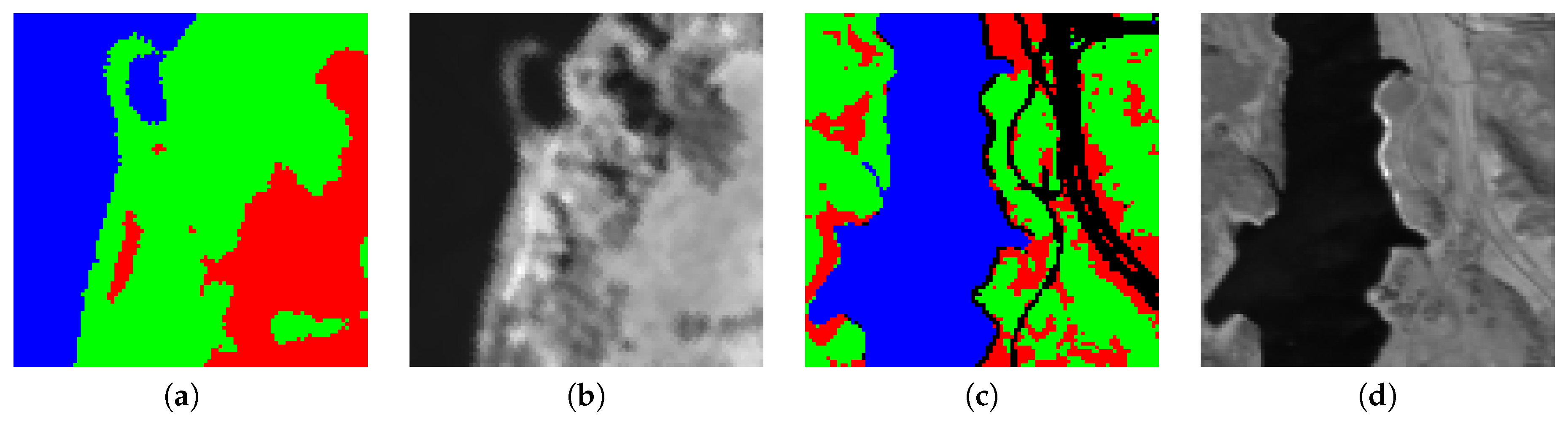
Figure 3 shows the partitions of Samson (a) and Jasper Ridge (c). In Samson, the three clusters shown in Figure 3a correspond to materials: Soil (red), Tree (green), and Water (blue). In Jasper Ridge, the four clusters shown in Figure 3c correspond to materials: Road (black), Soil (red), Water (blue), and Tree (green). According to the abundances shown in [33], the partitions of these two images are approximately correct. However, some of their clusters contain a significant number of highly mixed pixels (i.e., pixels in which more than one endmember has a significant abundance). Thus, in Samson, many of the pixels assigned to the cluster Tree are mixed pixels of Soil and Tree; and, in Jasper, many pixels assigned to the cluster Road are mixed pixels of Road and Soil (according to the abundance images shown in [33]).
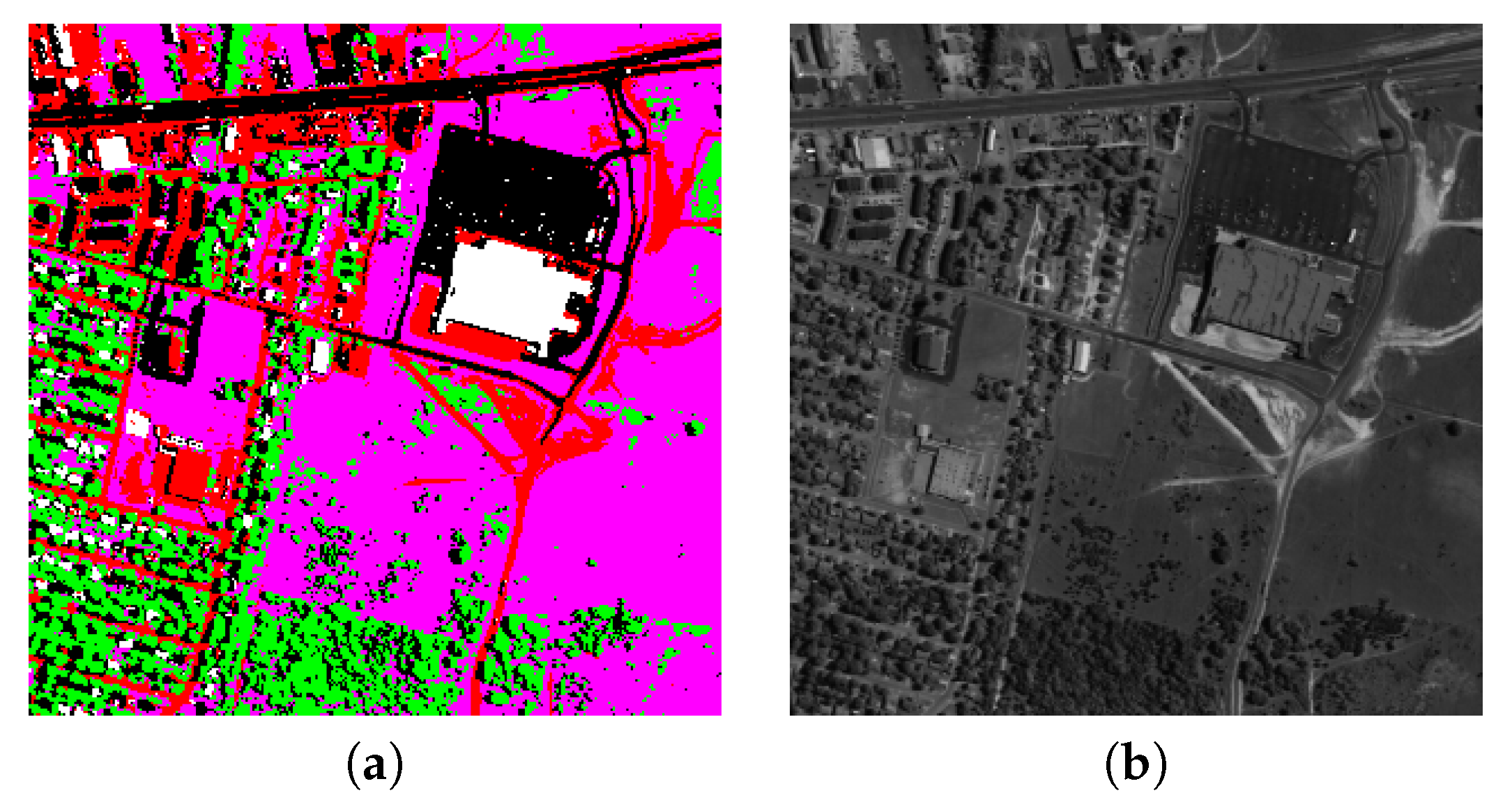
Figure 4a shows the partition for Urban. According to the abundances with five endmembers shown in [33], the clusters in that partition mainly correspond to materials: Asphalt (black), Roof (white), Grass (magenta), Tree (green), and Soil (red). Some material clusters, however, contain a significant number of pixels that correspond to other materials. For instance, many pixels with a high abundance of Asphalt in the ground truth of [33] are assigned to the cluster Soil in the partition.
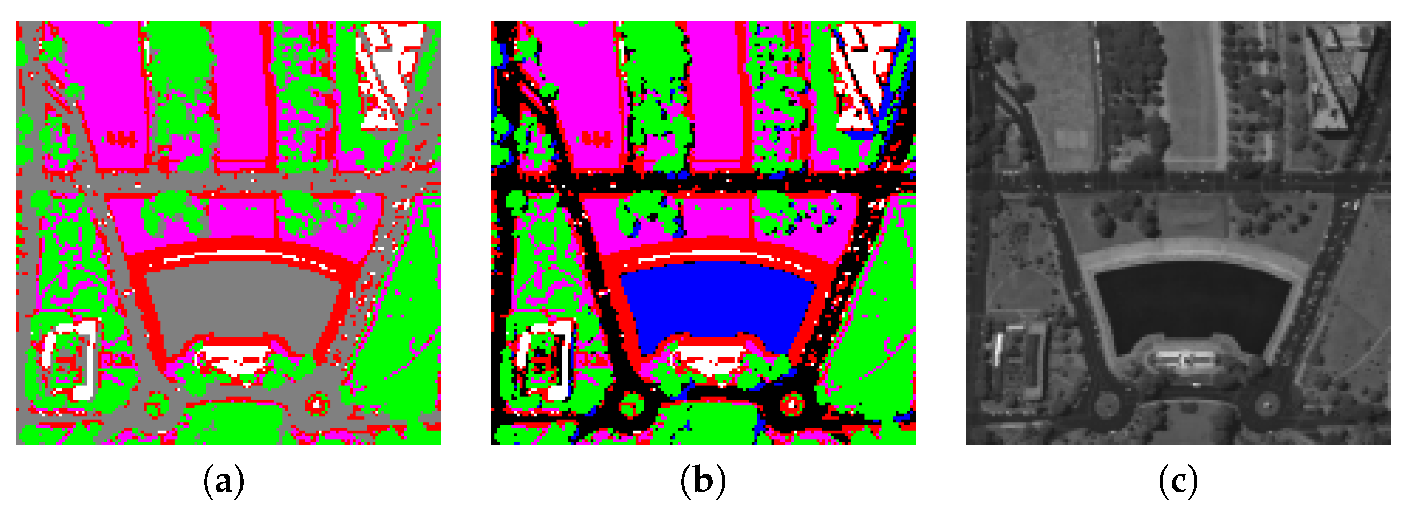
The image Washington DC has six materials, but the proposed method provides most times. The partition of that image with five clusters is shown in Figure 5a. According to the abundances shown in [33], the clusters of that partition approximately correspond to materials: Roof (white), Grass (magenta), Trail (red), Tree (green), and Road plus Water (gray). Hence, this partition joins the materials Road and Water into a single cluster. In the partition with six clusters, shown in Figure 5b, the materials Road (black) and Water (blue) each has its own cluster.
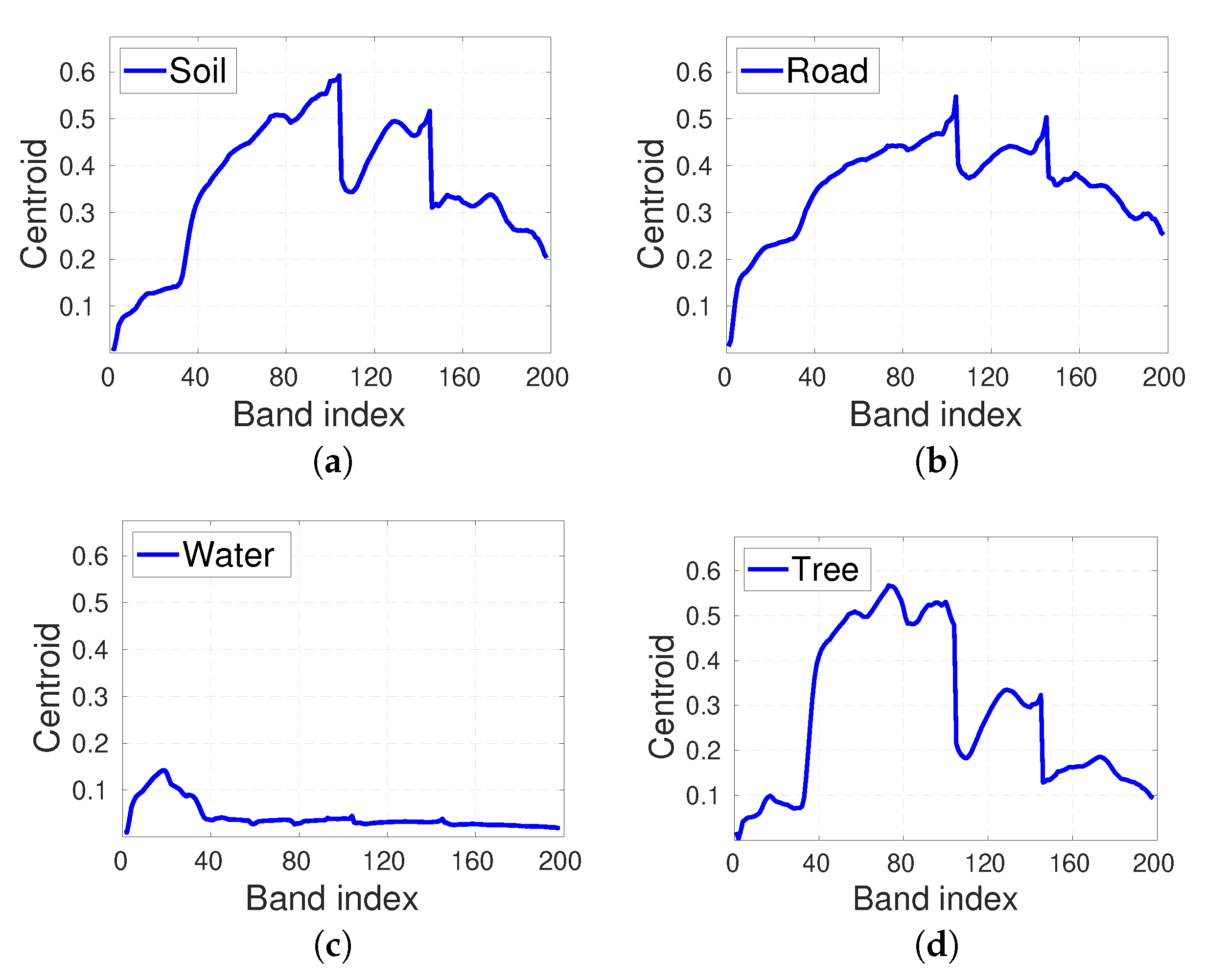
If a cluster of an image partition comprises all of the pixels that are mainly made of a certain material, the cluster centroid should be close to the endmember of that material. Hence, we can approximately obtain the endmembers of an image by computing the centroids of the clusters found by the proposed method. These centroids could serve as initial endmember approximations in unmixing applications. Figure 6, Figure 7, Figure 8 and Figure 9 show the cluster centroids of the partitions of Samson, Jasper Ridge, Urban, and Washinton DC, respectively. In Figure 7, the partition with 4 clusters has been used since is obtained most of the times in Jasper Ridge. Although was obtained in 24 out of 25 times, Figure 9 has been obtained using the partition with six clusters since, as mentioned above, this partition has a cluster for each of the six materials of the ground truth. In the following, we compare the centroids found in each image with the corresponding groundtruth endmembers shown in [32].
The cluster centroids of Samson (Figure 6) are very similar in shape to the corresponding endmembers shown in [32]. The centroid of Tree has a much smaller amplitude than its endmember in [32]. This is probably due to the fact that many pixels of this cluster are mixed pixels of Tree and Water and of Tree and Soil (in [32], the endmembers of Water and Soil have a smaller amplitude than that of Tree).
In Jasper Ridge (Figure 7), Road is the only cluster whose centroid significantly departs from its corresponding endmember in [32]. This centroid has a strong resemblance with that of Soil suggesting that many pixels assigned to the cluster Road belong to Soil or are mixed pixels of Road and Soil.
In Urban (Figure 8), Asphalt is the only cluster whose shape significantly differs from the endmember shown in [32]. Moreover, the centroid of Soil has much less amplitude than the endmember in [32] because many pixels of Asphalt (whose endmember has small and almost constant amplitude) are incorrectly assigned to Soil (see Figure 4c).
In Washington DC (Figure 8), the centroids of Water, Road and Tree are close to their corresponding ground truth endmembers of [32]. Larger differences are found between the centroids of Roof, Grass and Trail and their corresponding ground truth endmembers. This difference is significant in Roof which is justified by the fact that many of its pixels are mainly composed of the material Trail.
5. Discussion
Since K-means is initialized at random, we may obtain different values of when the algorithm is executed several times on the same image. By repeating K-means a number of times and choosing the partition with the minimum cost, we improve the quality of the estimate and also reduce its variability. The results have shown that when , repeating K-means 15 times provides good estimates of and with small variability.
Apart from the value of , it is also interesting to know whether the partition selected by the proposed method corresponds to a correct clustering of the image into its constituent materials. Note that since the partition is a hard classification of the input image, its clusters will generally contain mixed pixels. Moreover, clusters may contain misclassified pixels, that is, pixels that clearly should have been assigned to a different cluster. Both mixed and misclassified pixels have been found in the partitions shown in Section 4. When , we have shown that most clusters of the selected partition are good approximations of the true clusters of the image. When , the error can be due to the clustering or to the validation. Thus, in Washington DC ( and ), the paritition with six clusters is approximately correct but the validation erroneously selects the partition with five clusters.
Unlike other algorithms devised to estimate K, the proposed method also allows us to estimate the image endmembers by computing the cluster centroids of the selected partition. In the cluster of a certain material, mixed pixels and misclassified pixels may be very different from the material endmember. Nevertheless, when the percentage of these troublesome pixels is small, we can expect that the cluster centroid will be close to the corresponding endmember. This has been verified experimentally in Section 4.
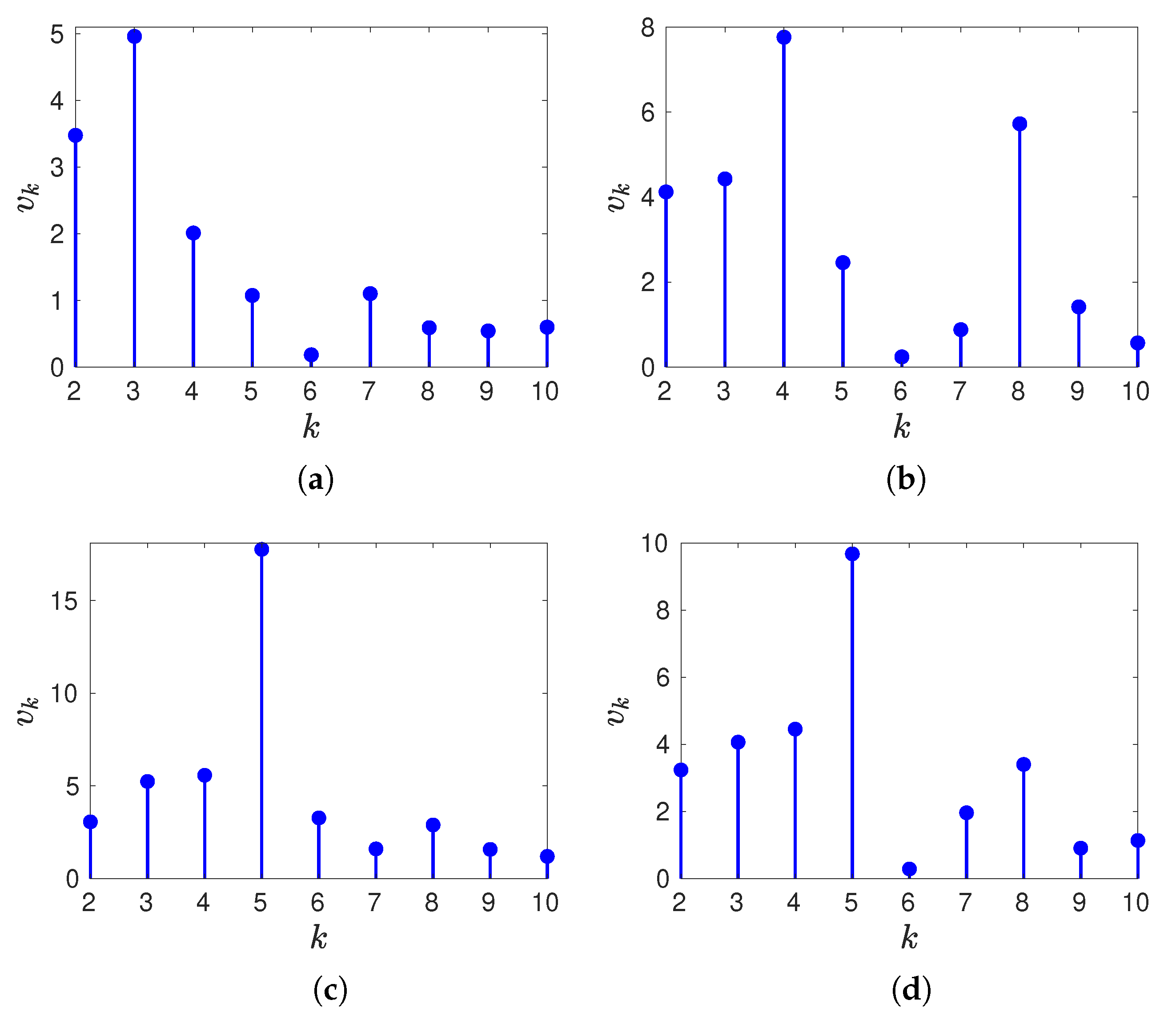
The validation step selects the integer k at which sequence is maximum. Figure 10 shows sequence obtained for each test image in one of the runs. For , all four sequences are increasing (as expected) even though the values are not very different. For , the sequences do not decrease monotonically (and in Jasper Ridge there is a large local maxima at ). Note that in Washington DC (Figure 10d), sequence has its minimum value at (when, according to the groundtruth, this image has six endmembers). However, in each of the four test images, the partition with a number of clusters equal to the number of endmembers is approximately correct.
Finally, we evaluate the efficiency of the proposed method but using standard partitional clustering algorithms and validation indexes. We have considered three standard clustering techniques: K-means (with the squared Euclidean distance), spherical K-means [39], and non-negative matrix factorization (NMF). In NMF, the largest component of the abundance vector of a pixel determines the cluster that is assigned to that pixel. As validation indexes, we have used the Davies-Bouldin index, the Calinski-Harabasz index, the Dunn index, and the average Silhouette index since these indexes are frequently used with partitional clustering algorithms [21,22]. For each clustering algorithm and validation index, we first obtained the image partition using the clustering algorithm with clusters, and then we selected the partition with the best validation index (the number of clusters of the optimal partition was set to ). Repeating the experiment (for each clustering algorithm, validation index, and image) generally provides the same value except in a few cases (in these cases, the median of the values is shown in Table 5).
Note in Table 5 that K is underestimated in many cases and that, in fact, the smallest possible value () is chosen in 50% of the cases. Underestimation is especially frequent when Spherical K-means is used as the clustering algorithm. No combination of clustering algorithm and validation index provides a good estimate of K in all four images, although K-means with the Calinski-Harabasz index provide good results except in the Samson image. The proposed method provides more accurate estimates than any of the twelve algorithms considered in Table 5.
6. Conclusions
We have presented an algorithm that estimates the number of endmembers of a hyperspectral image using agglomerative clustering. After building a hierarchy of image partitions, the proposed method selects the one that maximizes a validation index and sets the number of endmembers to the number of clusters of the selected partition. Our approach is conceptually different from previous techniques, most of which analyze the eigenvalues of the image correlation matrix. Moreover, our method also allows us to approximately obtain the endmembers of the image materials. Experimental results have shown that, for the set of test images considered, the proposed method provides better estimates than other well-known algorithms. The performance of our method depends on both the accuracy of the clustering and the effectiveness of the validation. Future work should focus on the search for a better validation index. Another line of future work is the use of the posterior probabilities of the clusters for each pixel. At each step of the hierarchy, these probabilities can be easily computed and constitute soft partitions of the input image that could improve both the estimation of K and the computation of the endmembers.
Author Contributions
Conceptualization, G.S., A.S. and L.V.; formal analysis, G.S., A.S., J.P. and L.V.; software, G.S., A.S. and J.P.; investigation, J.P., G.S. and A.S.; writing—original draft preparation, J.P.; writing—review and editing, J.P., A.S. and L.V. All authors have read and agreed to the published version of the manuscript.
Funding
This work was supported by Spanish Administration (Ministerio de Ciencia, Innovación y Universidades) and European Union (FEDER) under grant TEC2017-84743-P.
Conflicts of Interest
The authors declare no conflict of interest.
Appendix A. Estimation of Entropy and Cross-Entropy
In this appendix, we describe how to estimate . From (16), we can write
where the term , called the entropy of , is
and the term , called the cross-entropy of and , is
Now, we express the terms of (A1) as a function of the source variables, the mixing matrices, and the bias vectors of and . Since we model cluster with , where is square and invertible, and the random variables of are independent, we can write the entropy term in the form [40]
where is the entropy of the source variable , that is,
Let us now consider the cross-entropy term of (A1). Since and , cluster densities and can be written as
where and are the densities of source vectors and , respectively. Substituting (A6) into (A3) and making the change of variable , we obtain
where
Substituting the expressions found for , , , and into (A1), yields
Now, we describe how to approximate each term of the above expression. To obtain the terms (), the integral in (A5) is approximated using Monte Carlo integration:
where the values of the sequence are the elements of the i-th row of . Since this density is unknown, we estimate it from using kernel-density estimation [41]. Specifically, we use a Gaussian kernel:
where a is a normalization constant and ( is the standard deviation of . The approximation of the terms () is done in a similar way.
Finally, we show how and are approximated. First, consider the term defined in (A8) and assume that () is a sequence of Q vectors sampled from the density of random vector . We can approximate the integral in (A9) using Monte Carlo integration, that is,
where is obtained from with
Since is a vector of independent random variables, we have
where, similarly to what was done to evaluate (A10), each densities is estimated using a Gaussian kernel and the values of sequence (i.e., the elements of the i-th row of ). In our method, we have used .
The vectors of sequence are obtained by sampling from . Since is composed of M independent random variables, each variable can be sampled separately from the rest. Specifically, each sampled sequence () is obtained by using inverse transform sampling [42] where the inverse cumulative distribution is estimated from its available samples using kernel density estimation [41]. A similar procedure is used to estimate .
References
- Wang, L.; Zhao, C. Hyperspectral Image Processing; Springer: Berlin/Heidelberg, Germany, 2016. [Google Scholar]
- Keshava, N.; Mustard, J.F. Spectral Unmixing. IEEE Signal Process. Mag. 2002, 19, 47–57. [Google Scholar] [CrossRef]
- Harsanyi, J.; Farrand, W.; Chang, C.I. Determining the number and identity of spectral endmembers: An integrated approach using Neyman-Pearson eigenthresholding and iterative constrained RMS error minimization. In Proceedings of the 9th Thematic Conference on Geologic Remote Sensing, Pasadena, CA, USA, 8–11 February 1993. [Google Scholar]
- Bioucas-Dias, J.M.; Nascimento, J.M.P. Hyperspectral subspace identification. IEEE Trans. Geosci. Remote Sens. 2008, 46, 2435–2445. [Google Scholar] [CrossRef] [Green Version]
- Chang, C.I.; Du, Q. Estimation of number of spectrally distinct signal sources in hyperspectral imagery. IEEE Trans. Geosci. Remote Sens. 2004, 42, 608–619. [Google Scholar] [CrossRef] [Green Version]
- Cawse-Nicholson, K.; Damelin, S.B.; Robin, A.; Sears, M. Determining the intrinsic dimension of a hyperspectral image using random matrix theory. IEEE Trans. Image Process. 2013, 22, 1301–1310. [Google Scholar] [CrossRef] [PubMed]
- Halimi, A.; Honeine, P.; Kharouf, M.; Richard, C.; Tourneret, J.Y. Estimating the intrinsic dimension of hyperspectral images using noise-whitened eigengap approach. IEEE Trans. Geosci. Remote Sens. 2016, 54, 3811–3820. [Google Scholar] [CrossRef] [Green Version]
- Eches, O.; Dobigeon, N.; Tourneret, J.Y. Estimating the number of endmembers in hyperspectral images using the normal compositional model and a hierarchical bayesian algorithm. IEEE J. Sel. Top. Signal Process. 2010, 4, 582–591. [Google Scholar] [CrossRef] [Green Version]
- Berman, M. Improved estimation of the intrinsic dimension of a hyperspectral image using random matrix theory. Remote Sens. 2019, 11, 1049. [Google Scholar] [CrossRef] [Green Version]
- Roger, R. Principal components transform with simple, automatic noise adjustment. Int. J. Remote Sens. 1996, 17, 2719–2727. [Google Scholar] [CrossRef]
- Kritchman, S.; Nadler, B. Non-parametric detection of the number of signals: Hypothesis testing and random matrix theory. IEEE Trans. Signal Process. 2009, 57, 3930–3941. [Google Scholar] [CrossRef]
- Meer, P.; Jolion, J.M.; Rosenfeld, A. A fast parallel algorithm for blind estimation of noise variance. IEEE Trans. Pattern Anal. Mach. Intell. 1990, 12, 216–223. [Google Scholar] [CrossRef]
- Robin, A.; Cawse-Nicholson, K.; Mahmood, A.; Sears, M. Estimation of the intrinsic dimension of hyperspectral images: Comparison of current methods. IEEE J. Sel. Top. Appl. Earth Obs. Remote Sens. 2015, 8, 2854–2861. [Google Scholar] [CrossRef]
- Berman, M.; Hao, Z.; Stone, G.; Guo, Y. An investigation into the impact of band error variance estimation on intrinsic dimension estimation in hyperspectral images. IEEE J. Sel. Top. Appl. Earth Obs. Remote Sens. 2018, 11, 3279–3296. [Google Scholar] [CrossRef]
- Mahmood, A.; Robin, A.; Sears, M. Modified residual method for the estimation of noise in hyperspectral images. IEEE Trans. Geosci. Remote Sens. 2017, 55, 1451–1460. [Google Scholar] [CrossRef]
- Mahmood, A.; Robin, A.; Sears, M. Estimation of the noise spectral covariance matrix in hyperspectral images. IEEE J. Sel. Top. Appl. Earth Obs. Remote Sens. 2018, 11, 3853–3862. [Google Scholar] [CrossRef]
- Eismann, M.T.; Stein, D. Stochastic mixture modeling. In Hyperspectral Data Exploitation: Theory and Application; Chang, C.I., Ed.; Wiley: New York, NY, USA, 2007; Chapter 5; pp. 582–591. [Google Scholar]
- Hong, D.; Yokoya, N.; Chanussot, J.; Zhu, X.X. An augmented linear mixing model to address spectral variability for hyperspectral unmixing. IEEE Trans. Image Process. 2019, 28, 1923–1938. [Google Scholar] [CrossRef] [Green Version]
- Ma, Y.; Jin, Q.; Mei, X.; Dai, X.; Fan, F.; Li, H.; Huang, J. Hyperspectral unmixing with Gaussian mixture model and low-rank representation. Remote Sens. 2019, 11, 911. [Google Scholar] [CrossRef] [Green Version]
- Uezato, T.; Fauvel, M.; Dobigeon, N. Hierarchical sparse nonnegative matrix factorization for hyperspectral unmixing with spectral variability. Remote Sens. 2020, 12, 2326. [Google Scholar] [CrossRef]
- Everitt, B.S.; Landau, S.; Leese, M.; Stahl, D. Cluster Analysis, 5th ed.; Wiley: Chichester, UK, 2011. [Google Scholar]
- Xu, R.; Wunsch, R.C. Clustering; John Wiley and Sons: Hoboken, NJ, USA, 2009. [Google Scholar]
- Salazar, A.; Igual, J.; Vergara, L.; Serrano, A. Learning hierarchies from ICA mixtures. In Proceedings of the International Joint Conference on Neural Networks, Orlando, FL, USA, 12–17 August 2007; pp. 2271–2276. [Google Scholar]
- Lee, T.W.; Lewicki, M.S.; Sejnowski, T.J. ICA mixture models for unsupervised classification of non-Gaussian classes and automatic context switching in blind signal separation. IEEE Trans. Pattern Anal. Mach. Intell. 2000, 22, 1078–1089. [Google Scholar]
- Safont, G.; Salazar, A.; Vergara, L.; Gomez, E.; Villanueva, V. Multichannel dynamic modeling of non-Gaussian mixtures. Pattern Recognit. 2019, 93, 312–323. [Google Scholar] [CrossRef]
- Hyvärinen, A.; Karhunen, J.; Oja, E. Independent Component Analysis; Wiley-Interscience: New York, NY, USA, 2001. [Google Scholar]
- Kullback, S. Information Theory and Statistics; Dover: Minneola, NY, USA, 1968. [Google Scholar]
- Martínez-Usó, A.; Pla, F.; Sotoca, J.M.; García-Sevilla, P. Clustering-based hyperspectral band selection using information measures. IEEE Trans. Geosci. Remote Sens. 2007, 45, 4158–4171. [Google Scholar] [CrossRef]
- Carvalho, N.C.R.L.; Bins, L.S.; Sant’Anna, S.J.S. Analysis of stochastic distances and Wishart mixture models applied on PolSAR images. Remote Sens. 2019, 11, 2994. [Google Scholar] [CrossRef] [Green Version]
- Mojena, R. Hierarchical grouping methods and stopping rules: An evaluation. Comput. J. 1977, 20, 359–363. [Google Scholar] [CrossRef] [Green Version]
- Jain, A.K.; Dubes, R.C. Algorithms for Clustering Data; Prentice Hall: Englewood Cliffs, NJ, USA, 1988. [Google Scholar]
- Zhu, F. Hyperspectral Unmixing: Ground Truth Labeling, Datasets, Benchmark Performances and Survey. arXiv 2017, arXiv:1708.05125. [Google Scholar]
- Zhu, F.; Wang, Y.; Fan, B.; Xiang, S.; Meng, G.; Pan, C. Spectral unmixing via data-guided sparsity. IEEE Trans. Image Process. 2014, 23, 5412–5427. [Google Scholar] [CrossRef] [Green Version]
- Qian, Y.; Jia, S.; Zhou, J.; Robles-Kelly, A. Hyperspectral unmixing via sparsity-constrained nonnegative matrix factorization. IEEE Trans. Geosci. Remote Sens. 2011, 49, 4282–4297. [Google Scholar] [CrossRef] [Green Version]
- Wang, Y.; Pan, C.; Xiang, S.; Zhu, F. Robust hyperspectral unmixing with correntropy-based metric. IEEE Trans. Image Process. 2015, 24, 4027–4040. [Google Scholar] [CrossRef]
- García, V.; Salazar, A.; Safont, A.G.; Vidal, A.; Vergara, L. Parallelization of an algorithm for automatic classification of medical data. LNCS 2019, 11538, 3–16. [Google Scholar]
- Fernandez-Beltran, R.; Plaza, A.; Plaza, J.; Pla, F. Hyperspectral unmixing based on dual-depth sparse probabilistic latent semantic analysis. IEEE Trans. Geosci. Remote Sens. 2018, 56, 6344–6360. [Google Scholar] [CrossRef]
- Sigurdsson, J.; Ulfarsson, M.O.; Sveinsson, J.R. Parameter estimation for blind ℓq hyperspectral unmixing using bayesian optimization. In Proceedings of the Workshop on Hyperspectral Image and Signal Processing: Evolution in Remote Sensing (WHISPERS), Amsterdam, The Netherlands, 23–26 September 2018. [Google Scholar]
- Dhillon, I.S.; Modha, D.S. Concept decompositions for large sparse text data using clustering. Mach. Learn. 2001, 42, 143–175. [Google Scholar] [CrossRef] [Green Version]
- Cover, T.M.; Thomas, J.A. Elements of Information Theory, 2nd ed.; Wiley-Interscience: Hoboken, NJ, USA, 2006. [Google Scholar]
- Silverman, B.W. Density Estimation for Statistics and Data Analysis; Chapman and Hall/CRC: Boca Raton, FL, USA, 1986. [Google Scholar]
- Devroye, L. Non-Uniform Random Variate Generation; Springer-Verlag: New York, NY, USA, 1986. [Google Scholar]
Figure 1.
Overview of the proposed method for the estimation of the number of endmembers of a hyperspectral image.
Figure 1.
Overview of the proposed method for the estimation of the number of endmembers of a hyperspectral image.

Figure 2.
Hyperspectral test images (the result of averaging the band images is displayed as a grayscale image): (a) Samson, (b) Jasper Ridge, (c) Urban, and (d) Washington DC.
Figure 2.
Hyperspectral test images (the result of averaging the band images is displayed as a grayscale image): (a) Samson, (b) Jasper Ridge, (c) Urban, and (d) Washington DC.

Figure 3.
Partitions for (a) Samson and (c) Jasper Ridge provided by the proposed algorithm (their average bands are also shown in (b) and (d) for reference). Materials in Figure 3a: Soil (red), Tree (green), and Water (blue). Materials in Figure 3c: Road (black), Soil (red), Water (blue), and Tree (green).

Figure 4.
(a) Clustering of Urban and (b) its averaged band. Materials in Figure 4a: Asphalt (black), Roof (white), Grass (magenta), Tree (green), and Soil (red).
Figure 4.
(a) Clustering of Urban and (b) its averaged band. Materials in Figure 4a: Asphalt (black), Roof (white), Grass (magenta), Tree (green), and Soil (red).

Figure 5.
Partitions of Washington DC with (a) five clusters and (b) six clusters. The average band of that image is also shown for reference (c). Materials in Figure 5a: Roof (white), Grass (magenta), Trail (red), Tree (green), and Road plus Water (gray). Materials in Figure 5b: Roof (white), Grass (magenta), Trail (red), Tree (green), Road (black) and Water (blue).

Figure 6.
Cluster centroids of the partition of Samson with clusters: (a) centroid of Water; (b) centroid of Soil; (c) centroid of Tree.
Figure 6.
Cluster centroids of the partition of Samson with clusters: (a) centroid of Water; (b) centroid of Soil; (c) centroid of Tree.

Figure 7.
Cluster centroids of the partition of Jasper Ridge with clusters: (a) centroid of Soil; (b) centroid of Road; (c) centroid of Water; (d) centroid of Tree.
Figure 7.
Cluster centroids of the partition of Jasper Ridge with clusters: (a) centroid of Soil; (b) centroid of Road; (c) centroid of Water; (d) centroid of Tree.

Figure 8.
Cluster centroids of the partition of Urban with clusters: (a) centroid of Roof; (b) centroid of Grass; (c) centroid of Soil; (d) centroid of Asphalt; (e) centroid of Tree.
Figure 8.
Cluster centroids of the partition of Urban with clusters: (a) centroid of Roof; (b) centroid of Grass; (c) centroid of Soil; (d) centroid of Asphalt; (e) centroid of Tree.

Figure 9.
Cluster centroids of the partition of Washington DC with 6 endmembers: (a) centroid of Water; (b) centroid of Roof; (c) centroid of Road; (d) centroid of Grass; (e) centroid of Trail; (f) centroid of Tree.
Figure 9.
Cluster centroids of the partition of Washington DC with 6 endmembers: (a) centroid of Water; (b) centroid of Roof; (c) centroid of Road; (d) centroid of Grass; (e) centroid of Trail; (f) centroid of Tree.

Figure 10.
Sequence for (a) Samson, (b) Jasper Ridge, (c) Urban, and (d) Washington DC.


Table 1.
Spatial dimensions and number of bands (in parentheses, the number of total bands) of each hyperspectral test image.
Table 1.
Spatial dimensions and number of bands (in parentheses, the number of total bands) of each hyperspectral test image.
| Image | Samson | Jasper Ridge | Urban | Washington DC |
|---|---|---|---|---|
| Spatial dimensions | ||||
| Number of bands | 156 (156) | 198 (224) | 162 (221) | 191 (224) |
Table 2.
Estimated number of endmembers () obtained in each image after executing our algorithm 25 times. The groundtruth value of K is also provided for comparison.
Table 2.
Estimated number of endmembers () obtained in each image after executing our algorithm 25 times. The groundtruth value of K is also provided for comparison.
| Image | Samson | Jasper Ridge | Urban | Washington DC |
|---|---|---|---|---|
| 3 | 4 (23), 6 (2) | 5 | 5 (24), 4 (1) | |
| K: | 3 | 4 | 4, 5, 6 | 6 |
Table 3.
Estimated number of endmembers in each test image using HFC, NWHFC, HySime, RMT, NWEGA, and the proposed method.
Table 3.
Estimated number of endmembers in each test image using HFC, NWHFC, HySime, RMT, NWEGA, and the proposed method.
| Image | Samson | Jasper Ridge | Urban | Washington DC |
|---|---|---|---|---|
| HFC () | 9 | 9 | 50 | 13 |
| HFC () | 8 | 9 | 37 | 10 |
| HFC () | 8 | 7 | 29 | 9 |
| NWHFC () | 8 | 12 | 37 | 21 |
| NWHFC () | 8 | 10 | 35 | 18 |
| NWHFC () | 6 | 9 | 32 | 18 |
| HySime | 43 | 18 | 27 | 21 |
| RMT | 90 | 22 | 54 | 41 |
| NWEGA | 65 | 7 | 37 | 15 |
| The proposed method | 3 | 4 | 5 | 5 |
Table 4.
Running times (in seconds) of each algorithm for each test image.
| Image | Samson | Jasper Ridge | Urban | Washington DC |
|---|---|---|---|---|
| HFC | 0.024 | 0.037 | 0.269 | 0.083 |
| NWHFC | 0.031 | 0.048 | 0.334 | 0.105 |
| HySime | 0.109 | 0.234 | 1.456 | 0.486 |
| RMT | 0.111 | 0.228 | 1.462 | 0.485 |
| NWEGA | 0.108 | 0.228 | 1.455 | 0.484 |
| The proposed method | 26.83 | 43.08 | 396.99 | 72.46 |
Table 5.
Estimated number of endmembers using three clustering algorithms (K-means, Spherical K-means, and NMF) and four validation indexes (DB: Davies-Bouldin, CH: Calinski-Harabasz; D: Dunn, AS: average Silhouette) in each test image.
Table 5.
Estimated number of endmembers using three clustering algorithms (K-means, Spherical K-means, and NMF) and four validation indexes (DB: Davies-Bouldin, CH: Calinski-Harabasz; D: Dunn, AS: average Silhouette) in each test image.
| Image | K-Means | Spherical K-Means | NMF | |||||||||
|---|---|---|---|---|---|---|---|---|---|---|---|---|
| DB | CH | D | AS | DB | CH | D | AS | DB | CH | D | AS | |
| Samson | 2 | 9 | 2 | 2 | 2 | 2 | 2 | 2 | 3 | 5 | 3 | 3 |
| Jarper Ridge | 2 | 3 | 2 | 2 | 2 | 2 | 2 | 2 | 3 | 4 | 4 | 4 |
| Urban | 8 | 4 | 2 | 2 | 2 | 2 | 2 | 2 | 2 | 2 | 2 | 2 |
| Washington DC | 8 | 6 | 3 | 3 | 6 | 3 | 3 | 3 | 3 | 3 | 3 | 3 |
Publisher’s Note: MDPI stays neutral with regard to jurisdictional claims in published maps and institutional affiliations. |
© 2020 by the authors. Licensee MDPI, Basel, Switzerland. This article is an open access article distributed under the terms and conditions of the Creative Commons Attribution (CC BY) license (http://creativecommons.org/licenses/by/4.0/).
Share and Cite
MDPI and ACS Style
Prades, J.; Safont, G.; Salazar, A.; Vergara, L. Estimation of the Number of Endmembers in Hyperspectral Images Using Agglomerative Clustering. Remote Sens. 2020, 12, 3585. https://doi.org/10.3390/rs12213585
AMA Style
Prades J, Safont G, Salazar A, Vergara L. Estimation of the Number of Endmembers in Hyperspectral Images Using Agglomerative Clustering. Remote Sensing. 2020; 12(21):3585. https://doi.org/10.3390/rs12213585
Chicago/Turabian StylePrades, José, Gonzalo Safont, Addisson Salazar, and Luis Vergara. 2020. "Estimation of the Number of Endmembers in Hyperspectral Images Using Agglomerative Clustering" Remote Sensing 12, no. 21: 3585. https://doi.org/10.3390/rs12213585
Note that from the first issue of 2016, this journal uses article numbers instead of page numbers. See further details here.