A Conditional Probability Interpolation Method Based on a Space-Time Cube for MODIS Snow Cover Products Gap Filling


1
College of Earth and Environmental Sciences, Lanzhou University, Lanzhou 730000, China
2
Northwest Institute of Eco-Environment and Resources, Chinese Academy of Sciences, Lanzhou 730000, China
3
Jiangsu Center for Collaborative Innovation in Geographical Information Resource Development and Application, Nanjing 210023, China
*
Author to whom correspondence should be addressed.
Remote Sens. 2020, 12(21), 3577; https://doi.org/10.3390/rs12213577
Submission received: 29 September 2020
/
Revised: 26 October 2020
/
Accepted: 27 October 2020
/
Published: 31 October 2020
Abstract
:Seasonal snow cover is closely related to regional climate and hydrological processes. In this study, Moderate Resolution Imaging Spectroradiometer (MODIS) daily snow cover products from 2001 to 2018 were applied to analyze the snow cover variation in northern Xinjiang, China. As cloud obscuration causes significant spatiotemporal discontinuities in the binary snow cover extent (SCE), we propose a conditional probability interpolation method based on a space-time cube (STCPI) to remove clouds completely after combining Terra and Aqua data. First, the conditional probability that the central pixel and every neighboring pixel in a space-time cube of 5 × 5 × 5 with the same snow condition is counted. Then the snow probability of the cloud pixels reclassified as snow is calculated based on the space-time cube. Finally, the snow condition of the cloud pixels can be recovered by snow probability. The validation experiments with the cloud assumption indicate that STCPI can remove clouds completely and achieve an overall accuracy of 97.44% under different cloud fractions. The generated daily cloud-free MODIS SCE products have a high agreement with the Landsat–8 OLI image, for which the overall accuracy is 90.34%. The snow cover variation in northern Xinjiang, China, from 2001 to 2018 was investigated based on the snow cover area (SCA) and snow cover days (SCD). The results show that the interannual change of SCA gradually decreases as the elevation increases, and the SCD and elevation have a positive correlation. Furthermore, the interannual SCD variation shows that the area of increase is higher than that of decrease during the 18 years.
1. Introduction
Snow cover has a high albedo, high emissivity, and an important impact on regional climate and energy variation [1,2,3]. Additionally, snow is considered to be one of the sensitive factors to reflect climate change, especially regarding precipitation and temperature [4,5,6,7]. To understand climate change interactions and predicting climate warming tendencies, it is imperative to monitor accurately the snow cover extent (SCE) [8]. Moreover, snow cover is also a critical water source and significantly influences the hydrological and biochemical processes in surrounding lowland areas [9,10,11]. Hence, investigation of the spatiotemporal characteristics of snow is meaningful for effective management of limited water resources.
Snow is a main water resource in northern Xinjiang, China, and there is long-term snow cover in winter [4]. Sufficient snowfall is beneficial for agricultural irrigation in spring and crop wintering, but it also brings about frequent snow disasters [12]. Due to the influence of topography and geomorphology, the distribution of snow cover is uneven in different regions and seasons. Therefore, it is necessary to generate cloud-free SCE products and analyze the spatiotemporal change in snow cover in northern Xinjiang, China.
Remote sensing has shown great advantages in monitoring snow cover in large-scale and rugged terrain regions. Depending on the data source, research on snow variations includes in situ-based analysis, microwave-based analysis, and optical-based analysis [13,14]. The in situ data, which provide accurate and long record point measurements, are suitable for the analysis of climate tendency [15,16]. However, in situ snow monitoring is too rare to adequately quantify snow variations [17,18]. Passive microwave remote sensing data are effective in monitoring the spatiotemporal variations in snow cover by the snow depth and the snow water equivalent. However, their spatial resolution is usually low (>1 km), and detailed snow information is not acquired from them [19,20].
In optical remote sensing data, the Moderate Resolution Imaging Spectroradiometer (MODIS), which is onboard the Terra and Aqua satellites, is widely used to detect snow cover change because it has a high temporal resolution, high spatial resolution (500 m), and high accuracy of binary snow cover products [21,22,23,24,25]. Yang et al. [8] compared the accuracy of the MOD/MYD10A1 snow products and the Interactive Multisensor Snow and Ice Mapping System (IMS) products, and showed that the daily MODIS snow cover products have better performance. However, the daily MODIS snow cover products have many spatial and temporal gaps that are mainly due to cloud contamination.
To remove MODIS cloud pixels, several methods have been proposed in recent decades. MOD10A2 and MYD10A2 generated an 8-day maximum SCE, which reduced the temporal resolution of the original data [26]. Multisource fusion methods make full use of the high spatial resolution of MODIS and the good cloud-penetrating capacity of microwave products to remove cloud; e.g., MODIS and the advanced microwave scanning radiometer for earth observing system (25 km) [27,28,29] and MODIS and IMS (4 km) [30] have been fused. These methods resample the coarse spatial resolution of microwave products to 500 m to replace the cloud pixels in the MODIS products, and the fusion reduces the spatial resolution and leads to some uncertainty due to the reclassification accuracy of the cloud pixel depending on the microwave products [31,32,33]. Meanwhile, other spatial filter and temporal filter methods have also been developed to recover cloud gaps. Parajka and Blöschl [34] first presented a cloud removal method with three steps: Terra and Aqua image combination (TAC), spatial filtering using the nearest neighbors, and temporal filtering. This method has been improved by incorporating the snow line, air temperature, elevation information, and so on [35,36,37]. However, all these cloud removal methods use only spatial and temporal information step by step and ignore some important neighborhood information at small spatiotemporal distances.
Dozier et al. [38] first proposed the concept of taking the snow cover variation as a space-time cube to fill cloud gaps in fractional snow cover. Huang et al. [39] established a hidden Markov random field framework to fill SCE gaps, which were also based on a space-time cube and the snow mapping accuracy reached 88.0% for gap-filled areas. A space-time cube can make full use of neighborhood information to recover the ground characteristics. Additionally, the conditional probability interpolation method [40,41] can effectively calculate the conditional probability of snow pixels being covered by clouds and meteorological data to remove clouds, but this method has limited capacity for removing clouds in areas with few in situ observations. Therefore, we propose a conditional probability interpolation method based on a space-time cube (STCPI) that combines the advantages of a space-time cube and conditional probability interpolation method to produce daily cloud-free MODIS SCE products. This method takes the conditional probability as the weight of the space-time neighborhood pixels to calculate the snow probability of the cloud pixels, and then the snow condition of the cloud pixels can be recovered by the snow probability. The process can fill all of the cloud gaps in the MODIS SCE products.
The generated daily cloud-free MODIS snow products can effectively quantify the spatial and temporal changes of snow cover in northern Xinjiang, China. Yang et al. [42] analyzed the change of snow cover in northern Xinjiang with site data, showing that snow cover increased from 1961 to 2017. Chen et al. [43] used MODIS 8-day synthetic product to analyze the correlation between snow cover and elevation in Xinjiang, China, and there are some other studies about the snow cover variation in Tianshan Mountains [44,45,46]. However, systematic analysis of the spatial and temporal variation of snow cover in northern Xinjiang, China, is still rare, and current analyses are mainly based on the site data and MODIS version 5 snow products. In MODIS version 5 snow products, snow is detected from clouds and other land cover types with the normalized difference snow index (NDSI) threshold of 0.4 [47,48]. Compared with version 5, the new MODIS version 6 products released in 2016 better handles atmospheric correction, cloud and snow misclassification, recovers Aqua band 6, and provides NDSI products. Many researchers assessed the MODIS version 6 snow products exhibited that an NDSI threshold of 0.1 provides the highest accuracy [49,50]. Therefore, it is necessary and urgent to carry out more accurate spatiotemporal analysis of snow cover in northern Xinjiang, China based on higher precision version 6 snow products.
As a result, we first propose a new cloud remove method to generate daily cloud-free MODIS SCE products. The validation procedure of this method is based on the cloud assumption method and Landsat–8 OLI images. Then, we investigate the snow cover spatiotemporal variation by the snow cover area (SCA) and snow cover duration (SCD) in northern Xinjiang, China, from 2001 to 2018.
2. Study Area and Data
2.1. Study Area
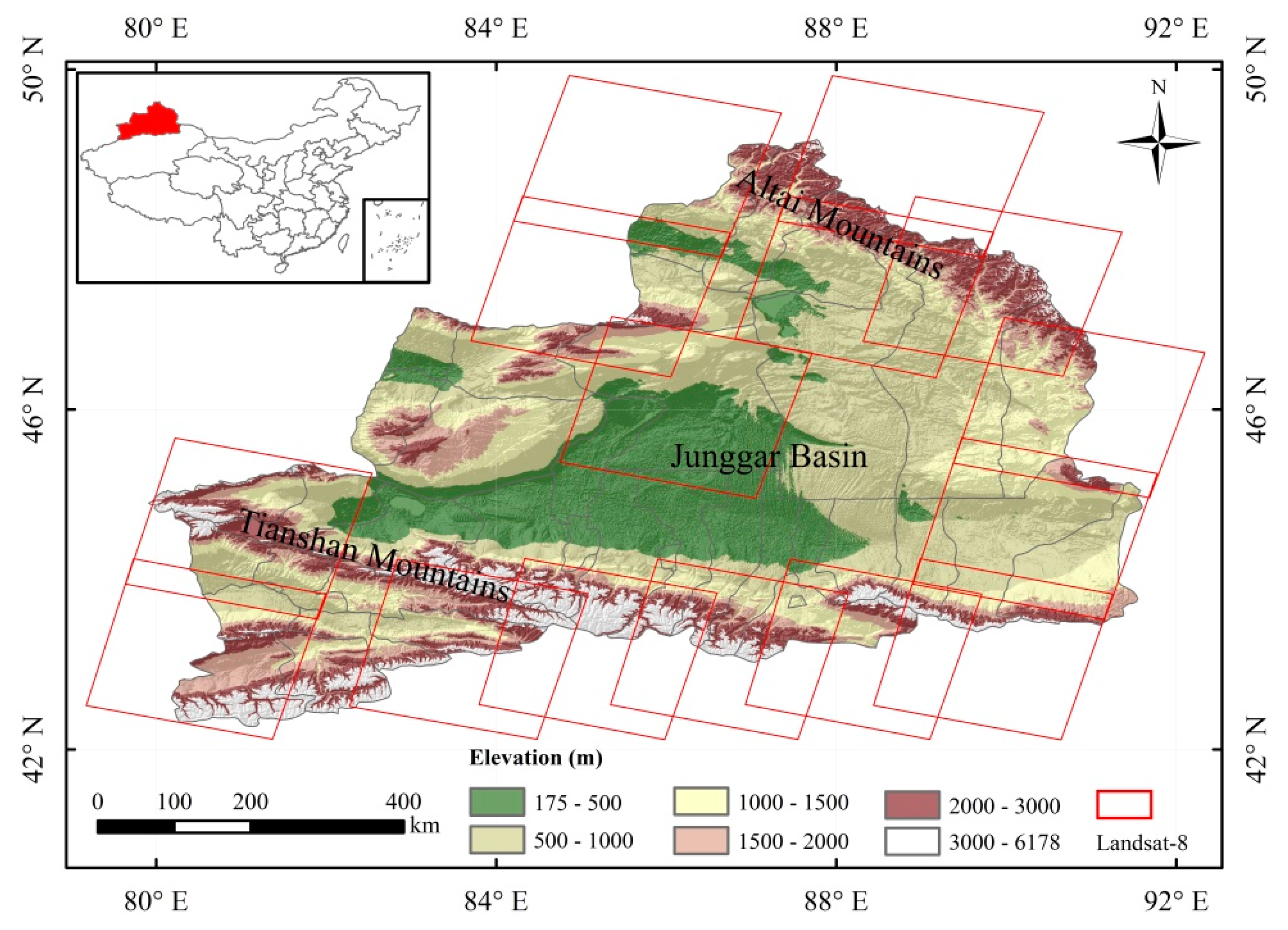
Northern Xinjiang, China, is located on the Eurasian continent in the range of 42°–50°N latitude and 79°–92°E longitude. This region covers a total area of 0.39 million km2 with an average elevation of 1256 m above sea level (Figure 1). The topographical features are the Junggar Basin situated in the middle of the region, and Altai Mountains and Tianshan Mountains are distributed on both sides of north and south. Due to a considerable amount of snowfall in this region, snow resources play a vital role in the water supply and ecosystem.
2.2. Data
Version 6 of the NDSI snow cover products in MOD/MYD10A1 was employed in this study. To conveniently fill in gaps, we reclassified the NDSI snow cover into three types–NDSI 0.1 was reclassified as snow; NDSI 0.1, inland water and ocean were reclassified as snow-free; the other classes (cloud, missing, no decision, night, detector saturated, and fill) were combined into a cloud class. The data were acquired from the Google Earth Engine (https://code.earthengine.google.com); there were 6556 images of MOD10A1 and 5959 images of MYD10A1 from 1 January 2001, to 31 December 2018.
Landsat–8 OLI data, which has a high spatial resolution of 30 m, were derived from the U.S. Geological Survey (USGS) (https://Earthexplorer.usgs.gov) to validate the produced daily cloud-free MODIS SCE products. Figure 1 shows the locations of the Landsat–8 OLI images.
Digital elevation data were derived from the Advanced Spaceborne Thermal Emission and Reflection Radiometer (ASTER) Global Digital Elevation Model (GDEM) version 2 with a 30 m spatial resolution. To match the MODIS snow products, the GDEM was resampled to 500 m grids by calculating the average elevation. These data were mainly used to analyze snow cover variation in different altitudinal zones.
3. Methodology
3.1. Gap-Filling Method
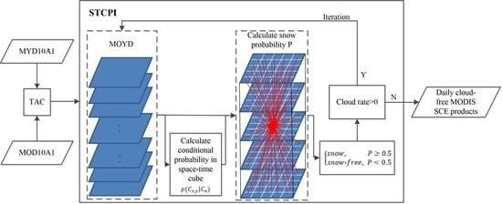
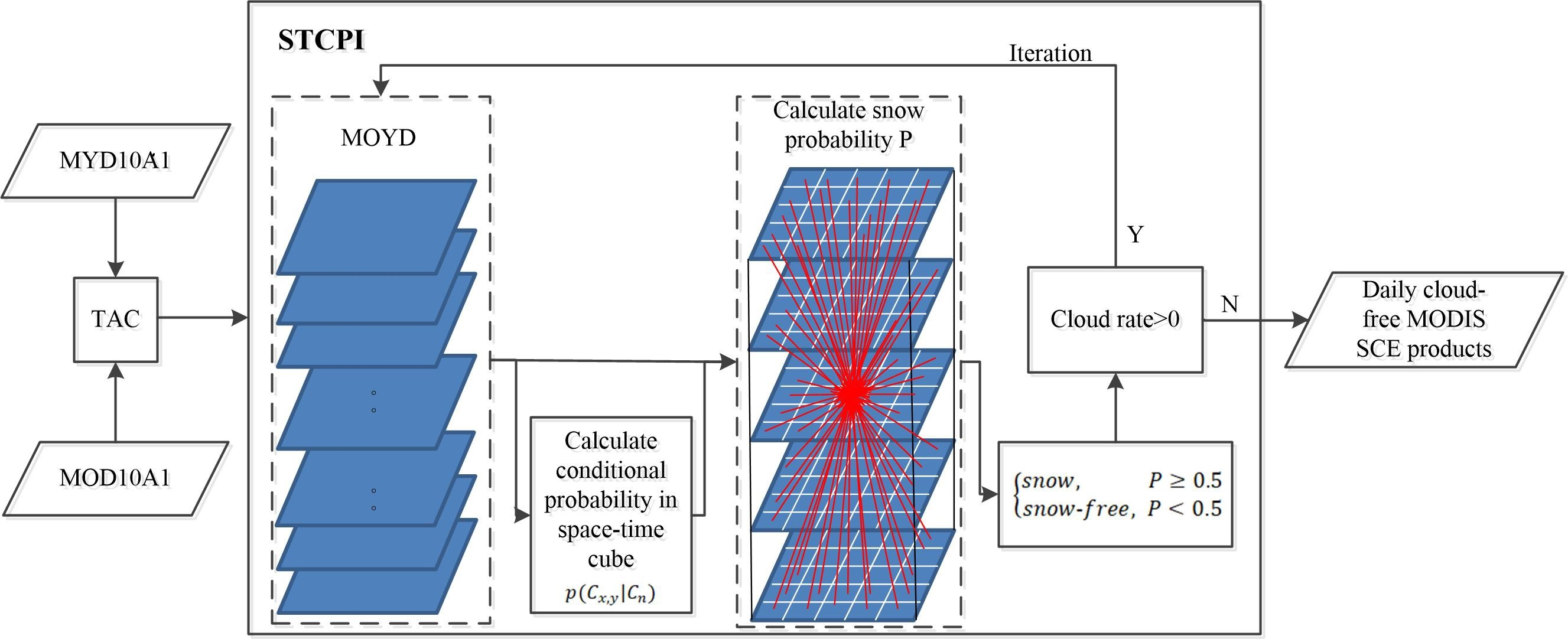
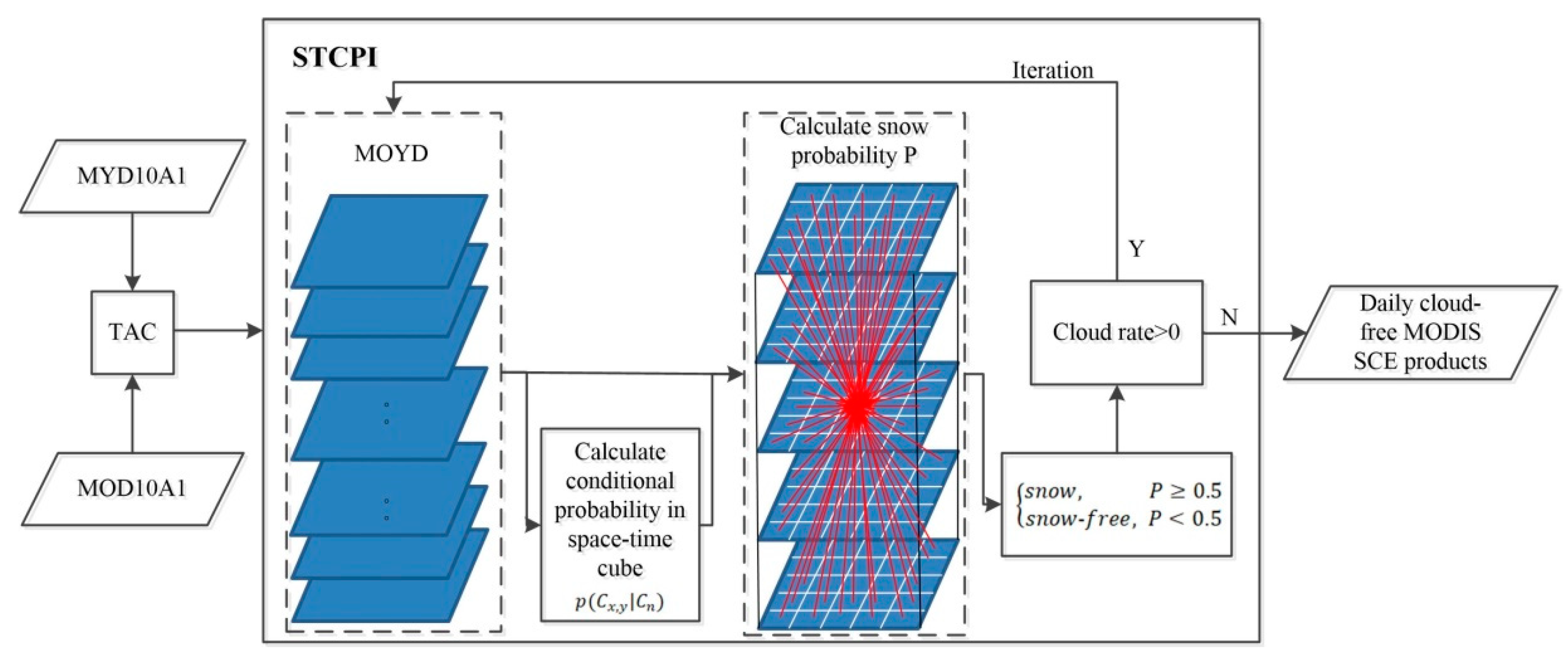
We propose a new gap-filling method that aims to produce daily cloud-free MODIS SCE products. First, TAC is used to remove partial cloud pixels, and then using STCPI method removed the remaining cloud completely. The cloud removal procedure is shown in Figure 2.
3.1.1. Terra and Aqua Daily Combination (TAC)
TAC has been used in many kinds of research to remove clouds [34,35,36,37,40]. As the Aqua and Terra satellites have different transit times but similar designs and performance, it is feasible to combine Terra (MOD10A1) and Aqua (MYD10A1) data to remove clouds. The combination rule is that first, when a pixel is snow in both MOD10A1 and MYD10A1, snow is taken as daily combination pixels; after that, when a pixel is snow-free in only one of the products, snow-free is taken as daily combination pixels; finally, the remainder pixels are taken as cloud for daily combination pixels [36]. Through defining snow > snow-free > cloud, this rule can be expressed as:
where x represents the row location, y represents the column location, and ST, SA, and SC represent the Terra, Aqua, and daily combination pixels, respectively. In this work, we refer to the daily combination products as MOYD.
3.1.2. Conditional Probability Interpolation Based on a Space-Time Cube (STCPI)
After TAC, there are still a large number of clouds in the MODIS SCE products. To fill the cloud gaps and ensure accuracy, STCPI is applied to recover snow conditions from the surrounding cloud-free pixels. This method takes the conditional probability as the weight of the space-time neighborhood pixels to calculate the snow probability of the cloud pixels, and then the snow condition of the cloud pixels can be recovered.
First, the conditional probability of each pixel in a clear sky is calculated, given that each pixel is in a space-time cube. The conditional probabilities are calculated using the following formula:
where is the conditional probability of the central pixel with coordinates x,y and the n-th neighboring pixel in the space-time cube having the same snow condition. and represent snow (C = 1) or snow-free (C = 0) conditions in the MODIS SCE products for days t and t´, respectively. Nx,y is the number of days in which the central pixel and n-th neighboring pixel are cloud-free over the study period 2001–2018. ranges from 0 to 1. The closer is to 1, the more consistent the changes in the n-th neighboring pixel and central pixel. That is, the n-th neighboring pixel and central pixel have a higher probability of having the same snow condition. Conversely, the closer is to 0, the greater the probability that the n-th neighboring pixel and central pixel have opposite snow conditions.
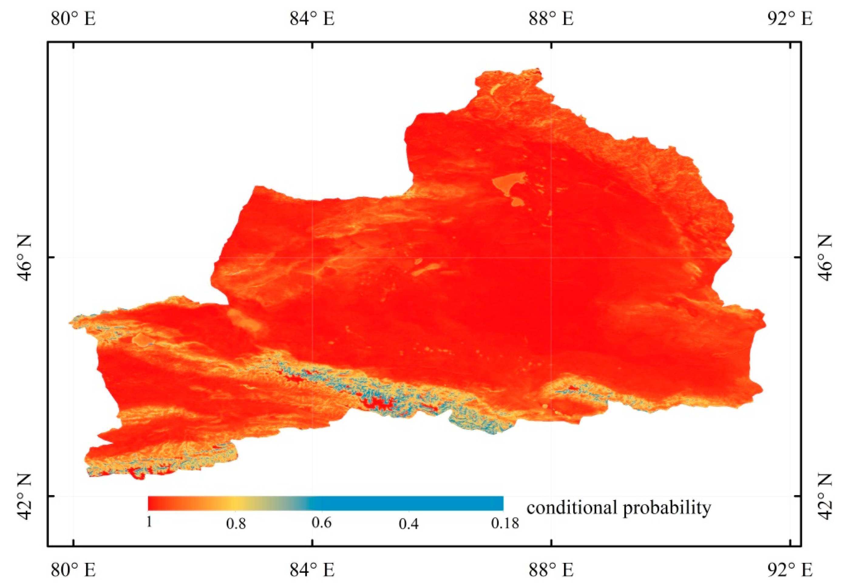
Figure 3 shows the conditional probability for the snow conditions of the central pixel with coordinates (x,y,t) and neighboring pixel with coordinates (x+2,y+2,t+2). The conditional probability in the mountains is lower than that on flat ground, especially in the Tianshan Mountains, because of the greater heterogeneity of the land surface in mountainous areas. To ensure that every central pixel has corresponding high conditional probability neighborhood pixels, and exclude the influence of low conditional probability neighborhood pixels to the final results, only the conditional probability is used to calculate the snow probability of the central pixel in this study. In general, the smaller the space-time distances between pixels, the greater the probability that they have the same snow condition. Therefore, it is necessary to select the smallest space-time cube with sufficient cloud-free neighborhood pixels. A too small space-time cube does not ensure sufficient cloud-free neighboring pixels to calculate the snow probability of central pixel, and a too big space-time cube will lead to more computational and time cost in the process of cloud removal. To maintain a small computational cost and ensure sufficient cloud-free pixels in the neighborhood space-time cube, the space-time cube of a 5 × 5 × 5 window (a spatial window of dimensions 5 × 5 and a time window of 5 days) was appropriate in this experiment.
Based on the conditional probability calculation in the space-time cube, we can use the current snow condition of the space-time cube to calculate the final snow probability ( of the cloud gaps:
where
As the range of snow probability is [0,1], and the real category of cloud pixels is only snow or snow-free, reconstructing cloud pixel information is a binary classification problem of judging cloud pixels to be snow or snow-free, which is an equal possibility event. Therefore, taking the median value of 0.5 as the threshold to judge the category of cloud is appropriate, and the snow condition can be determined by Equation (4). Then, the cloud pixels can be removed completely by performing STCPI iteration.
3.2. Validation Methodology
3.2.1. Validation Based on the Cloud Assumption
The truth snow condition in cloud gaps is unknown. Here, we apply a cloud assumption method to verify the gap-filling method [35,51,52]. The idea of the cloud assumption is to use clouds to mask the known SCE and then compare the recovered SCE with the known SCE to assess the performance of the cloud removal results.
3.2.2. Validation Based on Landsat–8 OLI Binary Snow Mapping
Binary snow maps retrieved from Landsat–8 OLI were used to verify the produced cloud-free MODIS SCE products. The SNOMAP algorithm defined a snow pixel as having NDSI ≥ 0.4 and the reflectance of near infrared (NIR) band ≥ 0.11 [47,53]. Due to the forest canopy obstructing the snow information from being transmitted to the sensor, the traditional method of snow cover mapping has low accuracy in a snow-covered forest [54,55]. To perform high-accuracy snow mapping in forest areas, a multi-index method focuses on snow-covered forests with NDSI < 0.4, making use of the normalized difference forest snow index (NDFSI) > 0.4 and the normalized difference vegetation index (NDVI) < 0.6 to extract forest snow; this method has an accuracy of more than 90% in northern Xinjiang, China [56]. Therefore, we used this method to extract the SCE from Landsat–8 OLI images and defined snow pixels as having NDSI ≥ 0.4 and NIR band≥0.11 or NDSI < 0.4, NDFSI > 0.4 and NDVI < 0.6. The normalized difference indexes are defined as follows:
where , , represent the reflectance of the shortwave infrared (SWIR), near infrared (NIR), green, and red bands in the Landsat–8 OLI image.
After that, we aggregate the Landsat–8 binary snow cover from 30 m to MODIS 500 m resolution to produce a fractional snow cover product, those pixels with fractional snow cover 15% are defined as snow, and others are snow-free [25,57,58,59]. Then, we validated the accuracy of the produced daily cloud-free MODIS SCE products.
3.2.3. Accuracy Assessment Metrics
The basic evaluation metrics based on the confusion matrix (Table 1) were applied to evaluate the results of the produced daily cloud-free MODIS SCE products; the metrics included the overestimation error (OE), underestimation error (UE), overall accuracy (OA), and F-score (Fs) [52,60]. OE is the probability that the recovered pixel is snow but the corresponding pixel in the true image is snow-free; UE is the probability that the recovered pixel is snow-free but the true pixel is snow; OA is defined by the number of correctly recovered pixels divided by the total number of pixels; Fs penalizes both the overestimation and underestimation of snow without the influence of extensive snow-free areas. The formulas for OE, UE, OA, and Fs are defined as follows:
3.3. Analysis of the Snow Cover Variation
Snow cover days (SCD) were calculated through the generated cloud-free MODIS SCE products, and the SCD is defined as the total number of days on which each pixel has snow in a given year. To capture the possible positive and negative trends of the snow cover variation and significance level, the Mann–Kendall and Theil–Sen median methods were conducted on each SCD series.
The Mann–Kendall method is a nonparametric statistical test method that is widely used to judge the significance of snow cover variation. This method does not need data that obey normal distribution, and it is not affected by a few outliers [6,61,62]. For a series Xi = (X1, X2,⋯ ⋯, Xn) with n samples, the specific formula is expressed as follows:
where
Additionally, n, m, and ti are the number of years, tied groups, and data values in the p-th group, respectively. The test statistic Z was used for the two-sided trend test when n > 10. Additionally, Z > 0 represents an upward trend, while Z < 0 represents a downward trend. As for significance level α, |Z| > Z1−α/2 represents a significant trend in the time series, otherwise it is nonsignificant; Z1−α/2 is acquired from the standard normal cumulative distribution table.
Theil–Sen median trend analysis is an effective nonparametric method for statistical trend variation, and the result is not greatly affected by abnormal values [63]. The calculation process of the Theil–Sen median slope for a series of length n is defined as follows:
where β > 0 and β < 0 represent an increasing and decreasing trend, respectively.
4. Results
4.1. Evaluation of the Gap-Filling Methods
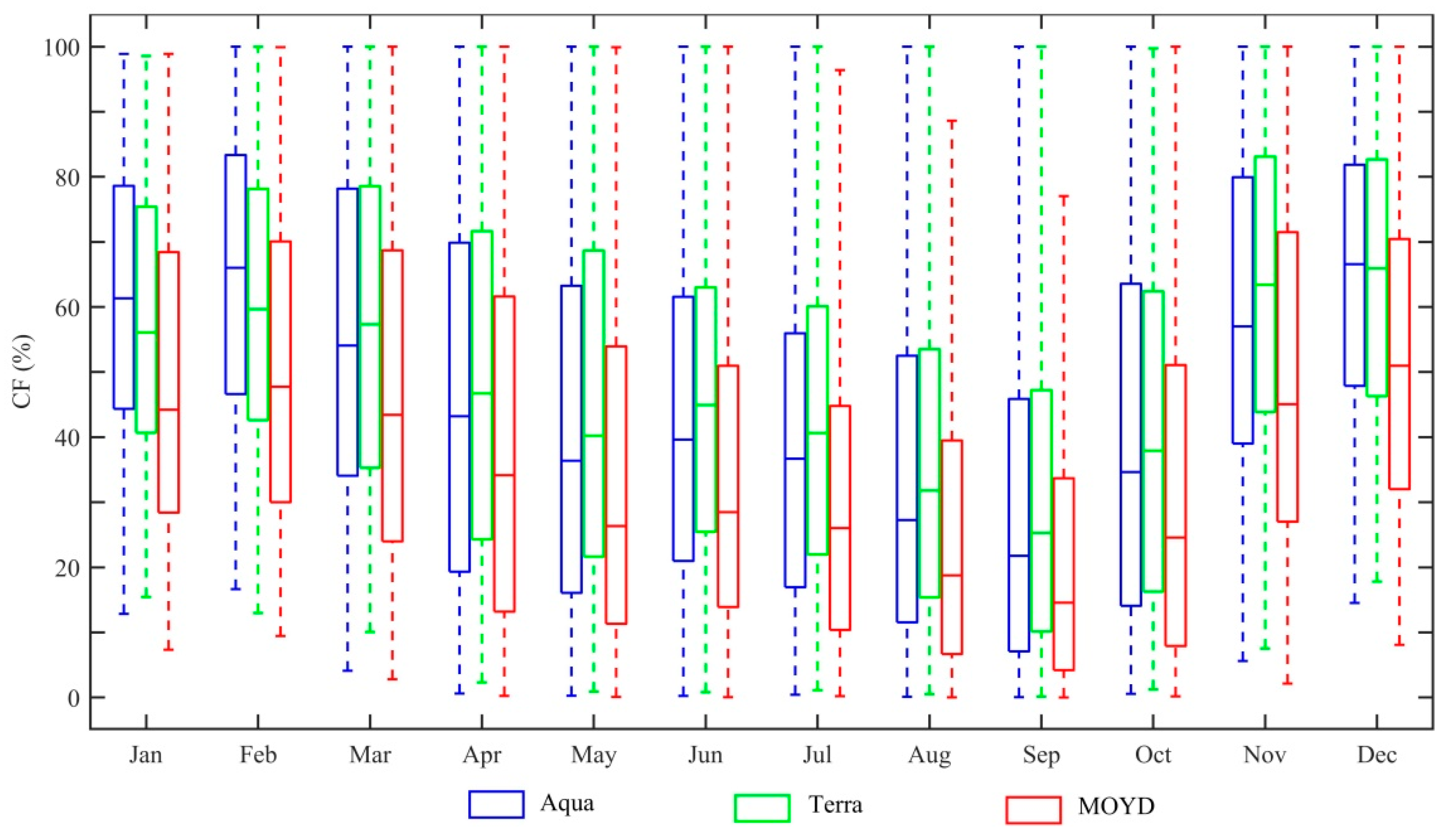
Based on the gap-filling method proposed in this paper, daily cloud-free MODIS SCE products for 2001–2018 in northern Xinjiang, China can be produced. Figure 4 shows the monthly variation in the cloud fraction (CF) for Terra, Aqua, and MOYD. For the original MODIS data, the CF of the Aqua products is similar to that of the Terra products. After TAC, the CF of MOYD is reduced by 8.99% on average compared to the Terra products. However, the remainder of the average CF is still 38.67%. Following STCPI, all the residual clouds are removed completely, and this method is effective in filling large cloud gaps. TAC has been extensively proven to have high accuracy, so we only evaluate the accuracy of STCPI for the generated daily cloud-free MODIS SCE products. The cloud assumption and Landsat–8 validation are implemented in the following.
4.1.1. Validation Based on the Cloud Assumption
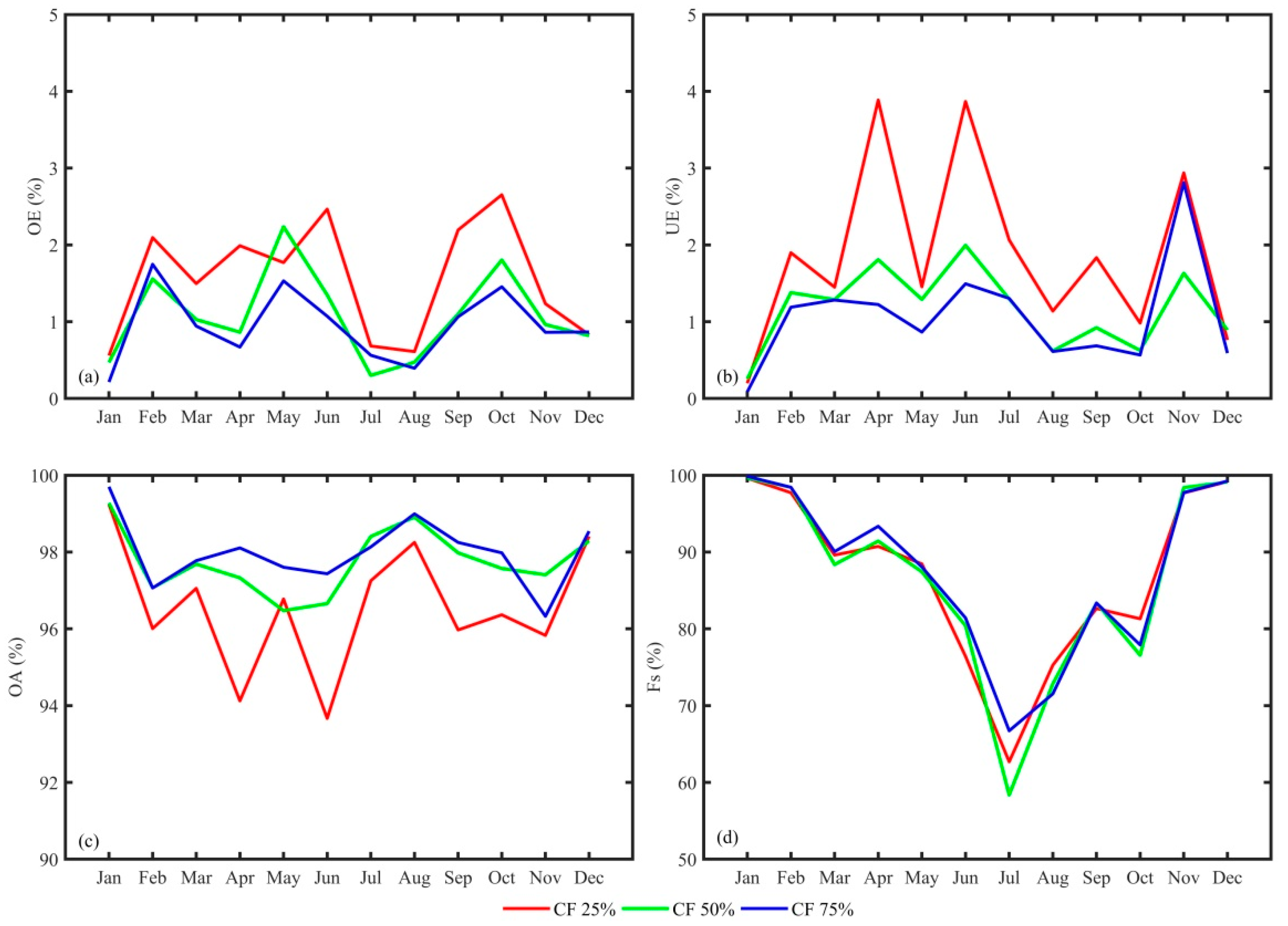
To evaluate the effectiveness of STCPI, the MOYD images with the lowest CF were selected in every month in 2018 as the true images, and a CF close to 25%, 50%, and 75% for every month in 2017 is applied to mask the true images. Figure 5 shows the STCPI prediction accuracy of the selected images. The average values of overestimation error, underestimation error, overall accuracy, and F-score are 1.19%, 1.37%, 97.44%, and 86.76%, respectively.
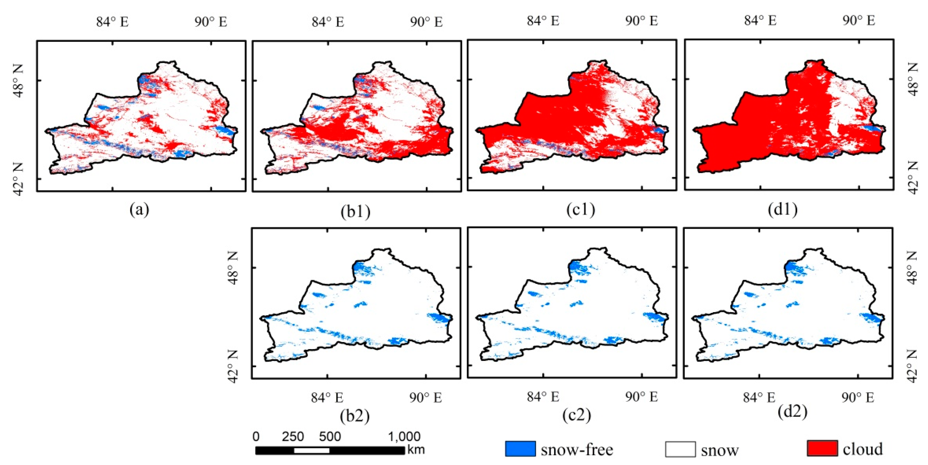
From Figure 5, we can draw the following four conclusions: (1) STCPI can effectively fill the gaps in binary snow cover and maintain high accuracy because OA maintains a high value all year. (2) The average OE is close to UE, which shows that the STCPI method does not lead to an overall overestimation or underestimation of the SCE. (3) Fs in summer is lower than that in winter, this is because the snow fraction of northern Xinjiang, China, is very small in summer, such as the snow fraction of only 2.35% on June 06, 2018. When there is little snow cover in summer and the image is covered by clouds, there is no effective neighborhood information that can be used to recover the snow information under the cloud coverage. This small part of the snow information recovery error does not affect the overall snow recovery results, which still have a high OA value. (4) A greater amount of CF shows better accuracy, which is related to the different spatial distribution of cloud-free pixels and the total number of cloud pixels for calculating accuracy. The recovered the snow condition of the pixel masked by cloud based on the neighborhood spatiotemporal information is more likely to cause misclassification at the boundary between snow and snow-free pixels. The larger cloud fraction usually includes smaller proportion of boundary pixels, and so a better precision can be achieved. Meanwhile, the gap-filling accuracy of STCPI is similar for different CF, which indicates that the STCPI method can remove large gaps in binary snow cover effectively. Figure 6 shows an example: STCPI removes CFs of 25.06%, 57.77%, and 77.38% and has an OA value of 97.72%, 98.41%, and 98.43%, respectively. Compared with the true images, the snow cover information is perfectly recovered visually.
4.1.2. Validation Based on Landsat–8 OLI
Validation based on the cloud assumption can effectively evaluate the accuracy of the gap-filling method, but the accuracy of the generated daily cloud-free MODIS SCE products is influenced by the gap-filling method and the original MODIS snow classification method, so we further evaluate the daily cloud-free MODIS SCE products using Landsat–8 OLI. OE, UE, OA, and Fs were calculated to validate the accuracy of the daily cloud-free MODIS SCE products acquired in this study.
We selected a total of 20 Landsat–8 OLI images (CF < 5%) in northern Xinjiang, China, from 2018 for validation. Table 2 shows the accuracy of the four assessment indicators and the CF of MOYD. We found that the average OE, 6.96%, of the daily cloud-free MODIS SCE products is higher than the UE, 2.70%, based on Landsat–8 OLI validation, which may be affected by the accuracy of the binary snow cover generated by the NDSI threshold. However, on the whole, the generated SCE has a high agreement with the Landsat–8 OLI image, with OA and Fs values of 90.34% and 92.87%, respectively.
4.2. Snow Cover Variability
Based on the generated daily cloud-free MODIS SCE products, we analyzed the variability of snow cover over northern Xinjiang, China, from 2001 to 2018. The main characteristics include the intra-annual variability, spatial distribution, and interannual variability.
4.2.1. Intra-Annual Variability of Snow Cover
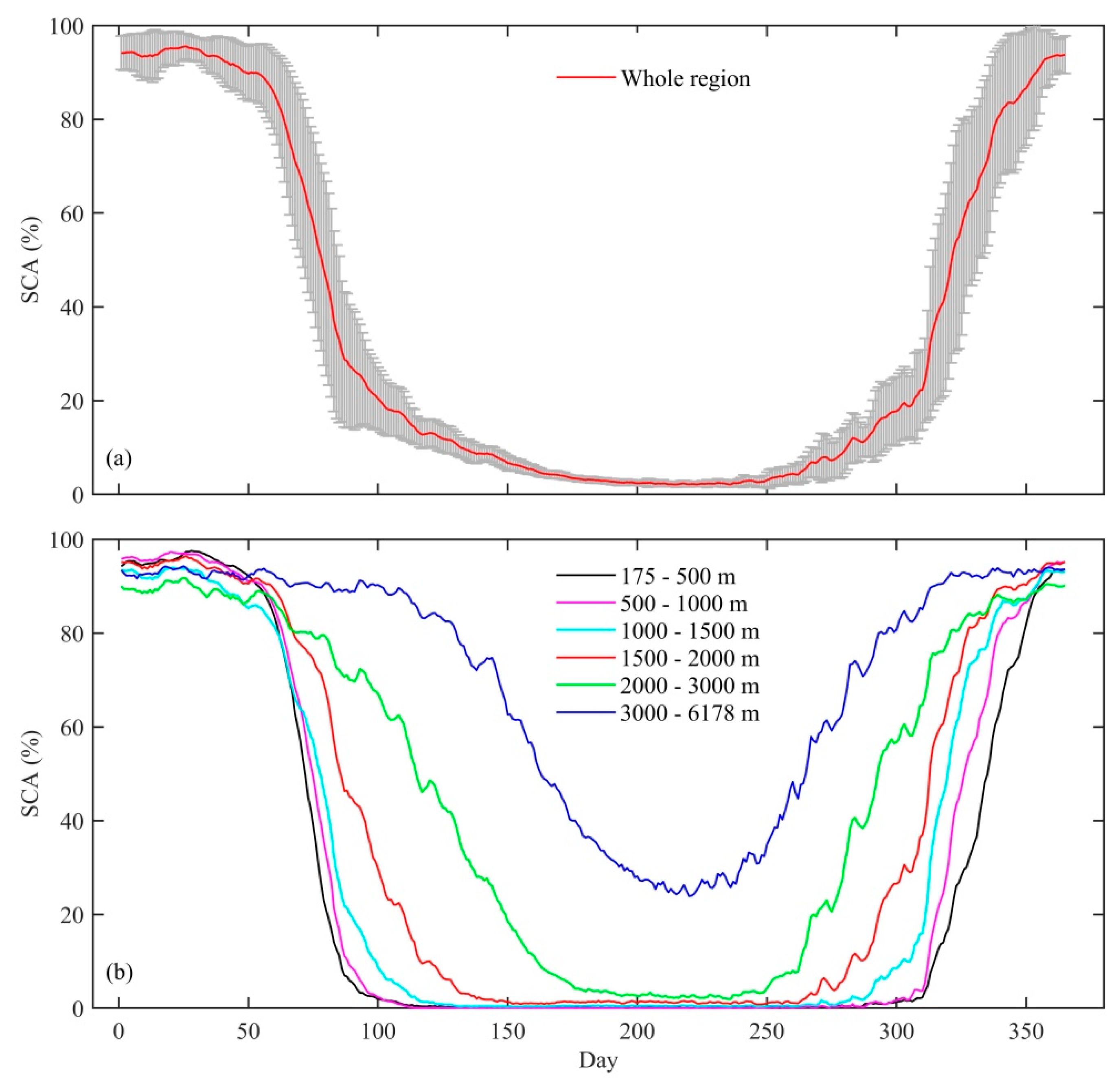
The SCA is widely used to analyze intra-annual snow cover changes. Figure 7 shows the time series of the daily SCA (%) for the whole region and six altitudinal zones from 2001 to 2018. The SCA in the study area has a strong seasonal variation. For all of northern Xinjiang, China, the SCA from December to February is greater than 60% as a stable snow period; in the March–April period, the SCA progressively decreases as snow melts; in the May–August period, the SCA is less than 5%; and in the September–November period, the SCA progressively increases as snow accumulation. From the perspective of the change in the standard deviation, the value in the May–August period is low, so the interannual fluctuation is slow, and the change is relatively large the rest of the time (Figure 7a).
At different altitudinal zones, the difference in SCA in terms of seasonal fluctuation shows obviously climatic characteristics (Figure 7b). On the whole, with the increase in elevation, the SCA increases gradually, the snowmelt period moves back, and the snow accumulation period moves forward. In the subregion with elevation > 3000 m, the lowest SCA is 23.88%, even in summer. Furthermore, 69.70% of northern Xinjiang, China, has an elevation < 1500 m, and the SCA variation in these areas has an obvious seasonal characteristic: the snow fraction is more than 80% in winter and close to 0 in summer.
4.2.2. Spatial Distribution of Snow Cover
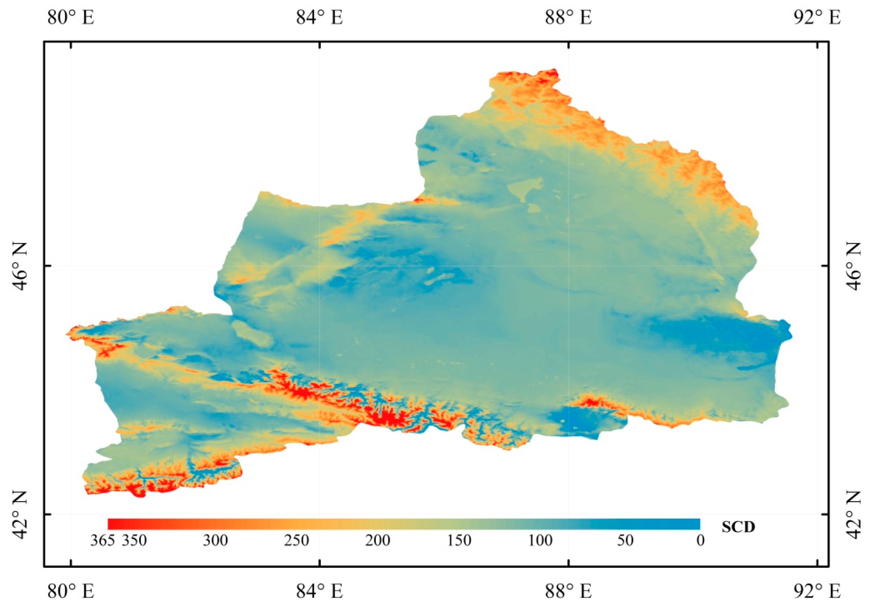
The mean SCD from 2001 to 2018 reflects the spatial distribution of the snow cover in northern Xinjiang, China (Figure 8). The average SCD and elevation have a positive correlation (r = 0.76), which shows that the SCD gradually increases as the elevation increases. SCD > 60 days, which is regarded as the stable SCA, occupies 96.64% of northern Xinjiang, China. Compared with the stable SCA, the unstable SCA, with SCD ≤ 60 days, occupies only 3.36%. The area with SCD > 200 days, occupying 10.85%, is mainly distributed in the Altai Mountains and the Tianshan Mountains.
4.2.3. Interannual Variability of Snow Cover
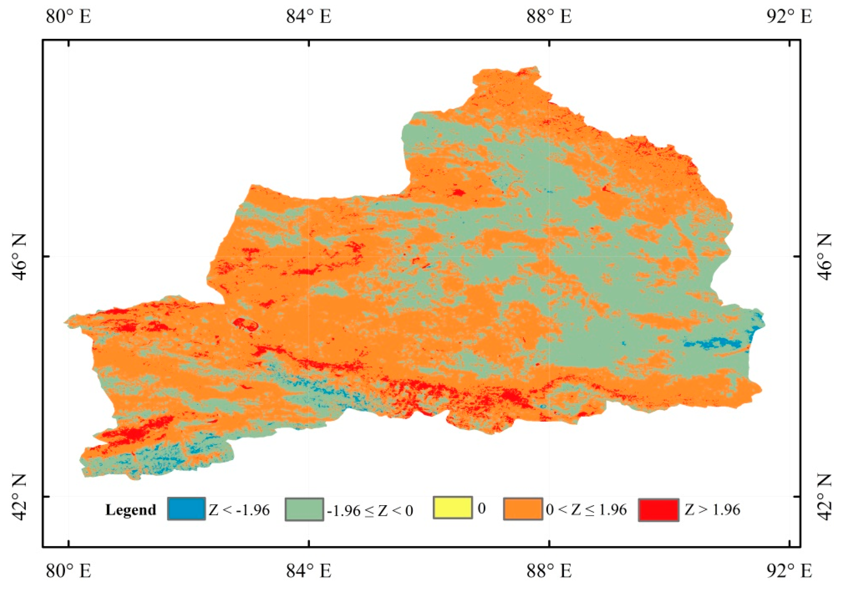
We used the Mann–Kendall and Sen’s median methods to analyze the trend and significance of SCD for northern Xinjiang, China, from 2001 to 2018 at the pixel scale. As shown in Figure 9, the SCD in 34.39% of the area decreased (Z < 0) during the 18 years and was mainly distributed in the Junggar Basin. The area of decrease was significant in 0.86% of the total area (Z < −1.96). In addition, the area with increasing SCD accounted for 59.96% of the total area, and 3.80% of the area experienced a significant increase; this region was mainly distributed in the Altai Mountains and the Tianshan Mountains. On the whole, SCD has a slight increasing trend in northern Xinjiang, China, from 2001 to 2018.
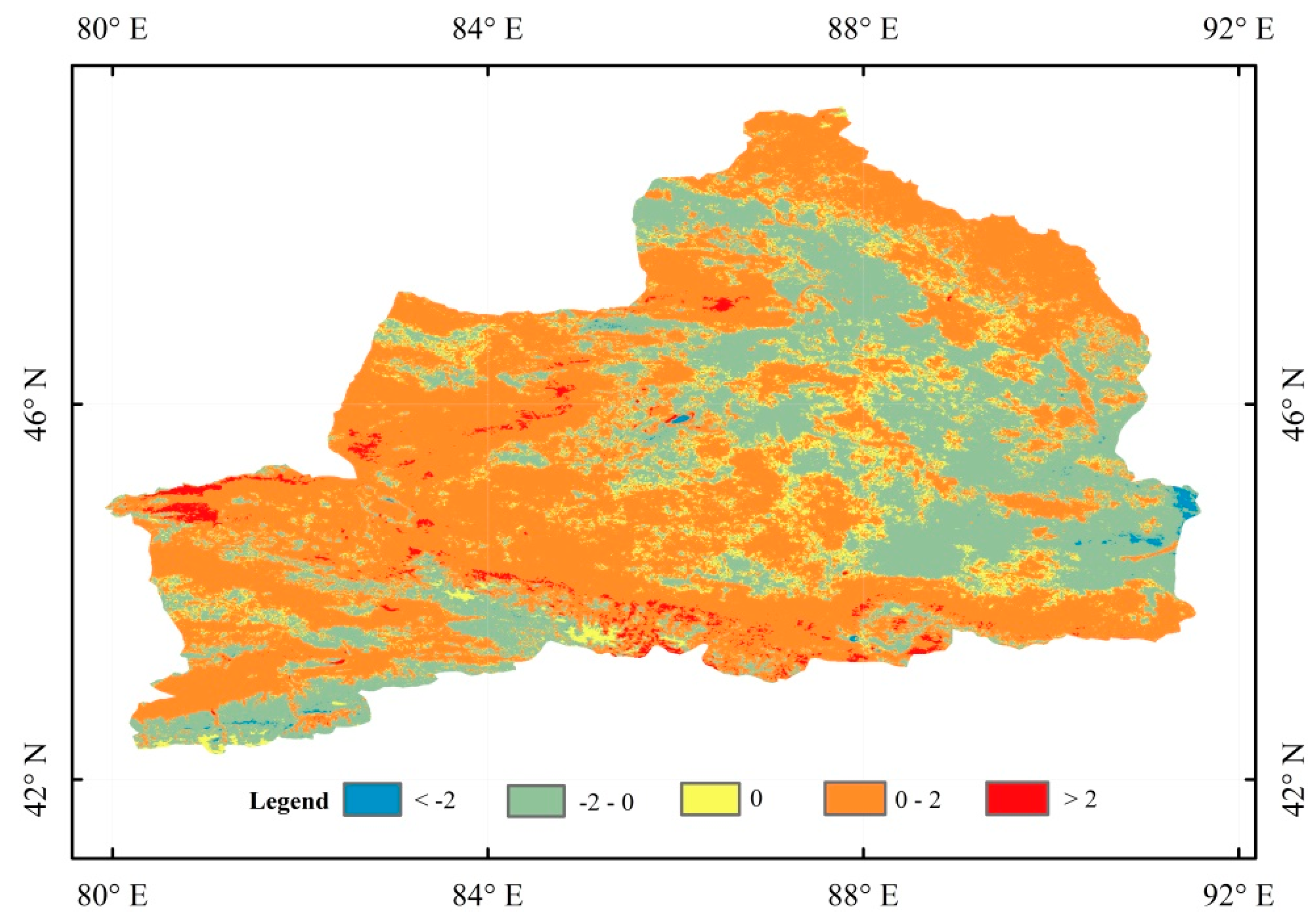
The slope of the SCD variation in northern Xinjiang, China, is shown in Figure 10. The SCD variation within 2 days/year has a proportion of 97.75%. In particular, the SCD shows an increased trend (β > 0) over 57.21% of the area, and the SCD shows a decreasing trend (β < 0) over 31.88% of the area. This also shows that the SCD has a slightly increased trend in northern Xinjiang, China, from 2001 to 2018, which is similar to the analysis result of the Mann–Kendall method. The increasing tendency of the SCD is consistent with previous studies that show snowfall has significantly increased in northern Xinjiang, China in the last few decades [12,64,65].
5. Discussion
MODIS version 6 snow products are used to generate daily cloud-free SCE products, and the accuracy of version 6 products is greatly improved compared with version 5 products due to better handling of atmospheric correction, cloud and snow misclassification, recovering Aqua band 6 [48]. Meanwhile, the original NDSI threshold of 0.4 applied in version 5 products has been proved by many studies to cause serious underestimation of snow cover in forest areas [55,66,67], which will reduce the credibility of the research on the spatial and temporal variation of snow cover. Based on MODIS version 6 products and NDSI threshold of 0.1, the accuracy of snow products is greatly improved. Therefore, a new cloud removal algorithm of STCPI is used to generate higher accuracy daily cloud-free MODIS SCE products.
STCPI can effectively fill large cloud gaps to generate SCE scenes, which may be attributed primarily to the following two advantages: (1) this method makes full use of adjacent space-time information; the spatial filter and temporal filter method uses spatiotemporal information step by step, which loses a large amount of information in the space-time cube, so it does not completely fill the cloud gaps in the image [13,68]. Conversely, STCPI makes full use of adjacent space-time information that can completely fill cloud gaps in one step and maintain high accuracy even with large cloud gaps in the image. (2) STCPI first calculates the conditional probability of the central pixel and every neighboring pixel in the space-time windows has the same snow condition. Generally, the closer the conditional probability is to 1, the more consistent the snow conditions of the neighboring pixels and central pixels [40]. The conditional probability established for fixed-position pixels is equivalent to considering the land cover, elevation, local environment information, and so on in the spatial neighborhood. Additionally, only a conditional probability > 0.8 was selected to calculate the snow probability of the central pixel because many neighboring pixels have different snow conditions from the central pixel, especially in mountain areas.
In addition, the STCPI shows that Fs in summer is lower than in winter in the validation of the cloud assumption. A difficult problem in image restoration is when there is little snow cover in summer and is covered by clouds [69], because there is no effective neighborhood information that can be used to recover the snow conditions under cloud coverage. This problem needs further study in the future. Moreover, the accuracy of the daily cloud-free MODIS SCE products is commonly influenced by the gap-filling method and the original MODIS snow classification method. Therefore, a higher-precision snow classification method can effectively improve the quality of the final daily cloud-free MODIS SCE products.
Under the background of global warming, snow cover change has a significant impact on social economy and regional climate. Therefore, it is very important to study the temporal and spatial changes of snow cover in northern Xinjiang, China. The snow cover has obvious seasonal variation trend in this region. The amount of snow cover is large in winter but little distribution in high altitude mountainous areas in summer. Chen et al. [43] and Li et al. [68] analyzed the relationship between snow cover and altitude, and showed that the distribution of snow cover had a clear positive correlation with altitude, we also obtained an correlation coefficient 0.76 in northern Xinjiang, China. Based on multivariate data fusion method among MODIS version 5 snow products, the advanced microwave scanning radiometer for earth observing system daily snow water equivalent products and IMS products, the analyses of the snow cover changes in northern hemisphere show that SCD of Altay Mountain and Tianshan Mountain is significantly reduced [32]. Tang et al. [44] generated cloud-free MODIS fractional snow cover products based on cubic spline function interpolation method and analyzed the SCD variation of Tianshan Mountain, they found that 26.39% of that region shows a downward trend and 34.26% shows a upward trend from 2001 to 2015. It is rare to use MODIS snow products to research the spatial and temporal variation of snow cover in northern Xinjiang, China. Yang et al. [42] and Wang et al. [12] analyzed the spatial-temporal changes of snow cover using the site data, and obtained the conclusion that the snowfall increased in northern Xinjiang, China, in the past decades, which is consistent with the slight increase trend of SCD in northern Xinjiang, China in this study.
6. Conclusions
This study proposed a new gap-filling method that produced high-precision daily cloud-free MODIS SCE products for northern Xinjiang, China, from 2001 to 2018 through TAC and STCPI. Through the validation of the cloud assumption, the OA of STCPI reached 97.44%. The OA of the final daily cloud-free MODIS SCE products is 90.34%, as validated by Landsat–8 OLI.
Based on the generated daily cloud-free MODIS SCE products, the snow cover variability was analyzed. The spatiotemporal variation characteristics of the snow cover from 2001 to 2018 provide further evidence for climate change in northern Xinjiang, China. It was found that the interannual change of SCA gradually decreases as the elevation increases and that the SCD has a positive correlation with elevation. Furthermore, based on Mann–Kendall and Sen’s median methods, we analyzed the changing tendency of the interannual snow cover. The results show that the area of SCD increase is higher than that of decrease during the 18 years. In the future, the relationship between snow cover variation and temperatures needs to be analyzed in detail under the conditions of a warming climate.
Author Contributions
Conceptualization, S.C. and X.W.; methodology, S.C. and X.W.; validation, S.C. and H.G.; writing—original draft preparation, S.C.; writing—review and editing, X.W., P.X., J.W. and X.H. All authors have read and agreed to the published version of the manuscript.
Funding
This research received no external funding.
Acknowledgments
This research was funded by the National Natural Science Foundation of China (No. 41771373, 41971325) and the Science and Technology Basic Resources Investigation Program of China (No. 2017FY100500).
Conflicts of Interest
The authors declare no conflict of interest.
References
- Yang, M.X.; Wang, X.J.; Pang, G.J.; Wang, G.N.; Liu, Z.C. The Tibetan Plateau cryosphere: Observations and model simulations for current status and recent changes. Earth Sci. Rev. 2019, 190, 353–369. [Google Scholar] [CrossRef]
- Kang, S.C.; Xu, Y.W.; You, Q.L.; Flugel, W.A.; Pepin, N.; Yao, T.D. Review of climate and cryospheric change in the Tibetan Plateau. Environ. Res. Lett. 2010, 5, 015101. [Google Scholar] [CrossRef]
- Xiao, C.D.; Qin, D.H.; Yao, T.D.; Ding, Y.J.; Liu, S.Y.; Zhao, L.; Liu, Y.J. Progress on observation of cryospheric components and climate-related studies in China. Adv. Atmos. Sci. 2008, 25, 164–180. [Google Scholar] [CrossRef]
- Tan, X.J.; Wu, Z.N.; Mu, X.M.; Gao, P.; Zhao, G.J.; Sun, W.Y.; Gu, C.J. Spatiotemporal changes in snow cover over China during 1960–2013. Atmos. Res. 2019, 218, 183–194. [Google Scholar] [CrossRef]
- Brown, R.D.; Mote, P.W. The Response of Northern Hemisphere Snow Cover to a Changing Climate. J. Clim. 2009, 22, 2124–2145. [Google Scholar] [CrossRef]
- Huang, X.; Deng, J.; Wang, W.; Feng, Q.; Liang, T. Impact of climate and elevation on snow cover using integrated remote sensing snow products in Tibetan Plateau. Remote Sens. Environ. 2017, 190, 274–288. [Google Scholar] [CrossRef]
- Keller, F.; Goyette, S.; Beniston, M. Sensitivity analysis of snow cover to climate change scenarios and their impact on plant habitats in alpine terrain. Clim. Chang. 2005, 72, 299–319. [Google Scholar] [CrossRef]
- Yang, J.T.; Jiang, L.M.; Menard, C.B.; Luojus, K.; Lemmetyinen, J.; Pulliainen, J. Evaluation of snow products over the Tibetan Plateau. Hydrol. Process. 2015, 29, 3247–3260. [Google Scholar] [CrossRef]
- Barnett, T.P.; Adam, J.C.; Lettenmaier, D.P. Potential impacts of a warming climate on water availability in snow-dominated regions. Nature 2005, 438, 303–309. [Google Scholar] [CrossRef]
- Zhang, G.Q.; Xie, H.J.; Yao, T.D.; Liang, T.G.; Kang, S.C. Snow cover dynamics of four lake basins over Tibetan Plateau using time series MODIS data (2001–2010). Water Resour. Res. 2012, 48. [Google Scholar] [CrossRef]
- Mingle, J. IPCC Special Report on the Ocean and Cryosphere in a Changing Climate. N. Y. Rev. Books 2020, 67, 49–51. [Google Scholar]
- Wang, S.; Ding, Y.; Jiang, F.; Anjum, M.N.; Iqbal, M. Defining Indices for the Extreme Snowfall Events and Analyzing their Trends in Northern Xinjiang, China. J. Meteorol. Soc. Jpn. Ser. II 2017, 95, 287–299. [Google Scholar] [CrossRef] [Green Version]
- Li, X.H.; Jing, Y.H.; Shen, H.F.; Zhang, L.P. The recent developments in cloud removal approaches of MODIS snow cover product. Hydrol. Earth Syst. Sci. 2019, 23, 2401–2416. [Google Scholar] [CrossRef] [Green Version]
- Frei, A.; Tedesco, M.; Lee, S.; Foster, J.; Hall, D.K.; Kelly, R.; Robinson, D.A. A review of global satellite-derived snow products. Adv. Space Res. 2012, 50, 1007–1029. [Google Scholar] [CrossRef] [Green Version]
- Egidijus, R.; Justas, K.; Sigita, B.; Indrė, G. Snow cover variability in Lithuania over the last 50 years and its relationship with large-scale atmospheric circulation. Boreal Environ. Res. 2014, 19, 337–357. [Google Scholar]
- Bulygina, O.N.; Razuvaev, V.N.; Korshunova, N.N. Changes in snow cover over Northern Eurasia in the last few decades. Environ. Res. Lett. 2009, 4, 045026. [Google Scholar] [CrossRef]
- Woo, M.K.; Thorne, R. Snowmelt contribution to discharge from a large mountainous catchment in subarctic Canada. Hydrol. Process. 2006, 20, 2129–2139. [Google Scholar] [CrossRef]
- Pu, Z.; Xu, L.; Salomonson, V.V. MODIS/Terra observed seasonal variations of snow cover over the Tibetan Plateau. Geophys. Res. Lett. 2007, 34. [Google Scholar] [CrossRef] [Green Version]
- Foster, J.L.; Hall, D.K.; Chang, A.T.C.; Rango, A. An Overview of Passive Microwave Snow Research and Results. Rev. Geophys. 1984, 22, 195–208. [Google Scholar] [CrossRef]
- Tait, A.B.; Hall, D.K.; Foster, J.L.; Armstrong, R.L. Utilizing Multiple Datasets for Snow-Cover Mapping. Remote Sens. Environ. 2000, 72, 111–126. [Google Scholar] [CrossRef]
- Hall, D.K.; Riggs, G.A. Accuracy assessment of the MODIS snow products. Hydrol. Process. 2007, 21, 1534–1547. [Google Scholar] [CrossRef]
- Klein, A.G.; Barnett, A.C. Validation of daily MODIS snow cover maps of the Upper Rio Grande River Basin for the 2000–2001 snow year. Remote Sens. Environ. 2003, 86, 162–176. [Google Scholar] [CrossRef]
- Maurer, E.P.; Rhoads, J.D.; Dubayah, R.O.; Lettenmaier, D.P. Evaluation of the snow-covered area data product from MODIS. Hydrol. Process. 2003, 17, 59–71. [Google Scholar] [CrossRef]
- Huang, X.D.; Liang, T.G.; Zhang, X.T.; Guo, Z.G. Validation of MODIS snow cover products using Landsat and ground measurements during the 2001–2005 snow seasons over northern Xinjiang, China. Int. J. Remote Sens. 2011, 32, 133–152. [Google Scholar] [CrossRef]
- Rittger, K.; Painter, T.H.; Dozier, J. Assessment of methods for mapping snow cover from MODIS. Adv. Water Resour. 2013, 51, 367–380. [Google Scholar] [CrossRef]
- Liang, T.; Huang, X.; Wu, C.; Liu, X.; Li, W.; Guo, Z.; Ren, J. An application of MODIS data to snow cover monitoring in a pastoral area: A case study in Northern Xinjiang, China. Remote Sens. Environ. 2008, 112, 1514–1526. [Google Scholar] [CrossRef]
- Gao, Y.; Xie, H.J.; Lu, N.; Yao, T.D.; Liang, T.G. Toward advanced daily cloud-free snow cover and snow water equivalent products from Terra-Aqua MODIS and Aqua AMSR-E measurements. J. Hydrol. 2010, 385, 23–35. [Google Scholar] [CrossRef]
- Huang, X.; Hao, X.; Feng, Q.; Wang, W.; Liang, T. A new MODIS daily cloud free snow cover mapping algorithm on the Tibetan Plateau. Sci. Cold Arid Reg. 2014, 6, 116–123. [Google Scholar] [CrossRef]
- Liang, T.G.; Zhang, X.T.; Xie, H.J.; Wu, C.X.; Feng, Q.S.; Huang, X.D.; Chen, Q.G. Toward improved daily snow cover mapping with advanced combination of MODIS and AMSR-E measurements. Remote Sens. Environ. 2008, 112, 3750–3761. [Google Scholar] [CrossRef]
- Yu, J.; Zhang, G.; Yao, T.; Xie, H.; Zhang, H.; Ke, C.; Yao, R. Developing Daily Cloud-Free Snow Composite Products From MODIS Terra–Aqua and IMS for the Tibetan Plateau. IEEE Trans. Geosci. Remote Sens. 2016, 54, 2171–2180. [Google Scholar] [CrossRef]
- Gao, Y.; Xie, H.J.; Yao, T.D.; Xue, C.S. Integrated assessment on multi-temporal and multi-sensor combinations for reducing cloud obscuration of MODIS snow cover products of the Pacific Northwest USA. Remote Sens. Environ. 2010, 114, 1662–1675. [Google Scholar] [CrossRef]
- Wang, Y.; Huang, X.; Liang, H.; Sun, Y.; Feng, Q.; Liang, T. Tracking Snow Variations in the Northern Hemisphere Using Multi-Source Remote Sensing Data (2000–2015). Remote Sens. 2018, 10, 136. [Google Scholar] [CrossRef] [Green Version]
- Hao, X.H.; Luo, S.Q.; Che, T.; Wang, J.; Li, H.Y.; Dai, L.Y.; Huang, X.D.; Feng, Q.S. Accuracy assessment of four cloud-free snow cover products over the Qinghai-Tibetan Plateau. Int. J. Digit. Earth 2019, 12, 375–393. [Google Scholar] [CrossRef]
- Parajka, J.; Blöschl, G. Spatio-temporal combination of MODIS images—Potential for snow cover mapping. Water Resour. Res. 2008, 44. [Google Scholar] [CrossRef]
- Gafurov, A.; B’ardossy, A. Cloud removal methodology from MODIS snow cover product. Hydrol. Earth Syst. Sci. 2009, 13, 1361–1373. [Google Scholar] [CrossRef] [Green Version]
- Paudel, K.P.; Andersen, P. Monitoring snow cover variability in an agropastoral area in the Trans Himalayan region of Nepal using MODIS data with improved cloud removal methodology. Remote Sens. Environ. 2011, 115, 1234–1246. [Google Scholar] [CrossRef]
- Kilpys, J.; Pipiraitė-Januškienė, S.; Rimkus, E. Snow climatology in Lithuania based on the cloud-free moderate resolution imaging spectroradiometer snow cover product. Int. J. Climatol. 2020. [Google Scholar] [CrossRef]
- Dozier, J.; Painter, T.H.; Rittger, K.; Frew, J.E. Time-space continuity of daily maps of fractional snow cover and albedo from MODIS. Adv. Water Resour. 2008, 31, 1515–1526. [Google Scholar] [CrossRef]
- Huang, Y.; Liu, H.; Yu, B.; Wu, J.; Kang, E.L.; Xu, M.; Wang, S.; Klein, A.; Chen, Y. Improving MODIS snow products with a HMRF-based spatio-temporal modeling technique in the Upper Rio Grande Basin. Remote Sens. Environ. 2018, 204, 568–582. [Google Scholar] [CrossRef]
- Dong, C.; Menzel, L. Producing cloud-free MODIS snow cover products with conditional probability interpolation and meteorological data. Remote Sens. Environ. 2016, 186, 439–451. [Google Scholar] [CrossRef]
- Gafurov, A.; Vorogushyn, S.; Farinotti, D.; Duethmann, D.; Merkushkin, A.; Merz, B. Snow-cover reconstruction methodology for mountainous regions based on historic in situ observations and recent remote sensing data. Cryosphere 2015, 9, 451–463. [Google Scholar] [CrossRef] [Green Version]
- Yang, T.; Li, Q.; Liu, W.; Liu, X.; Li, L.; De Maeyer, P. Spatiotemporal variability of snowfall and its concentration in northern Xinjiang, Northwest China. Theor. Appl. Climatol. 2019, 139, 1247–1259. [Google Scholar] [CrossRef]
- Chen, W.; Ding, J.; Wang, J.; Zhang, J.; Zhang, Z. Temporal and spatial variability in snow cover over the Xinjiang Uygur Autonomous Region, China, from 2001 to 2015. PeerJ 2020, 8, e8861. [Google Scholar] [CrossRef] [PubMed] [Green Version]
- Tang, Z.; Wang, X.; Wang, J.; Wang, X.; Li, H.; Jiang, Z. Spatiotemporal Variation of Snow Cover in Tianshan Mountains, Central Asia, Based on Cloud-Free MODIS Fractional Snow Cover Product, 2001–2015. Remote Sens. 2017, 9, 1045. [Google Scholar] [CrossRef] [Green Version]
- Yang, T.; Li, Q.; Ahmad, S.; Zhou, H.; Li, L. Changes in Snow Phenology from 1979 to 2016 over the Tianshan Mountains, Central Asia. Remote Sens. 2019, 11, 499. [Google Scholar] [CrossRef] [Green Version]
- Li, Y.; Chen, Y.; Li, Z. Climate and topographic controls on snow phenology dynamics in the Tienshan Mountains, Central Asia. Atmos. Res. 2020, 236, 104813. [Google Scholar] [CrossRef]
- Dozier, J. Spectral Signature of Alpine Snow Cover from the Landsat Thematic Mapper. Remote Sens. Environ. 1989, 28, 9–22. [Google Scholar] [CrossRef]
- Riggs, G.A.; Hall, D.K.; Román, M.O. MODIS Snow Products Collection 6 User Guide; National Snow and Ice Data Center: Boulder, CO, USA, 2015. [Google Scholar]
- Da Ronco, P.; Avanzi, F.; De Michele, C.; Notarnicola, C.; Schaefli, B. Comparing MODIS snow products Collection 5 with Collection 6 over Italian Central Apennines. Int. J. Remote Sens. 2020, 41, 4174–4205. [Google Scholar] [CrossRef]
- Zhang, H.B.; Zhang, F.; Zhang, G.Q.; Che, T.; Yan, W.; Ye, M.; Ma, N. Ground-based evaluation of MODIS snow cover product V6 across China: Implications for the selection of NDSI threshold. Sci. Total Environ. 2019, 651, 2712–2726. [Google Scholar] [CrossRef]
- Hou, J.; Huang, C.; Zhang, Y.; Guo, J.; Gu, J. Gap-Filling of MODIS Fractional Snow Cover Products via Non-Local Spatio-Temporal Filtering Based on Machine Learning Techniques. Remote Sens. 2019, 11, 90. [Google Scholar] [CrossRef] [Green Version]
- Chen, S.; Wang, X.; Guo, H.; Xie, P.; Sirelkhatim, A.M. Spatial and Temporal Adaptive Gap-Filling Method Producing Daily Cloud-Free NDSI Time Series. IEEE J. Sel. Top. Appl. Earth Obs. Remote Sens. 2020, 13, 2251–2263. [Google Scholar] [CrossRef]
- Hall, D.K.; Riggs, G.A.; Salomonson, V.V. Development of Methods for Mapping Global Snow Cover Using Moderate Resolution Imaging Spectroradiometer Data. Remote Sens. Environ. 1995, 54, 127–140. [Google Scholar] [CrossRef]
- Dagrun, V.; Rune, S. Subpixel mapping of snow cover in forests by optical remote sensing. Remote Sens. Environ. 2003, 84, 69–82. [Google Scholar]
- Klein, A.G.; Hall, D.K.; Riggs, G.A. Improving snow cover mapping in forests through the use of a canopy reflectance model. Hydrol. Process. 1998, 12, 1723–1744. [Google Scholar] [CrossRef]
- Wang, X.; Wang, J.; Che, T.; Huang, X.; Hao, X.; Li, H. Snow Cover Mapping for Complex Mountainous Forested Environments Based on a Multi-Index Technique. IEEE J. Sel. Top. Appl. Earth Obs. Remote Sens. 2018, 11, 1433–1441. [Google Scholar] [CrossRef]
- Metsämäki, S.; Mattila, O.-P.; Niemi, K. Continental use of SCAmod fractional snow cover mapping method in boreal forest and tundra belt. In Proceedings of the 2012 IEEE International Geoscience and Remote Sensing Symposium, Munich, Germany, 22–27 July 2012; pp. 1578–1581. [Google Scholar]
- Painter, T.H.; Rittger, K.; McKenzie, C.; Slaughter, P.; Davis, R.E.; Dozier, J. Retrieval of subpixel snow covered area, grain size, and albedo from MODIS. Remote Sens. Environ. 2009, 113, 868–879. [Google Scholar] [CrossRef] [Green Version]
- Hao, S.R.; Jiang, L.M.; Shi, J.C.; Wang, G.X.; Liu, X.J. Assessment of MODIS-Based Fractional Snow Cover Products over the Tibetan Plateau. IEEE J. Sel. Top. Appl. Earth Obs. Remote Sens. 2019, 12, 533–548. [Google Scholar] [CrossRef]
- Liu, C.; Li, Z.; Zhang, P.; Zeng, J.; Gao, S.; Zheng, Z. An Assessment and Error Analysis of MOD10A1 Snow Product Using Landsat and Ground Observations over China During 2000–2016. IEEE J. Sel. Top. Appl. Earth Obs. Remote Sens. 2020, 13, 1467–1478. [Google Scholar] [CrossRef]
- Guo, M.; Li, J.; He, H.; Xu, J.; Jin, Y. Detecting Global Vegetation Changes Using Mann-Kendal (MK) Trend Test for 1982–2015 Time Period. Chin. Geogr. Sci. 2018, 28, 907–919. [Google Scholar] [CrossRef] [Green Version]
- Chaudhuri, S.; Dutta, D. Mann-Kendall trend of pollutants, temperature and humidity over an urban station of India with forecast verification using different ARIMA models. Environ. Monit. Assess. 2014, 186, 4719–4742. [Google Scholar] [CrossRef]
- Theil, H. A Rank-Invariant Method of Linear and Polynomial Regression Analysis. In Henri Theil’s Contributions to Economics and Econometrics; Advanced Studies in Theoretical and Applied Econometrics; Raj, B., Koerts, J., Eds.; Springer: Dordrecht, The Netherlands, 1992; Volume 23. [Google Scholar] [CrossRef]
- Zhou, B.; Wang, Z.; Shi, Y.; Xu, Y.; Han, Z. Historical and Future Changes of Snowfall Events in China under a Warming Background. J. Clim. 2018, 31, 5873–5889. [Google Scholar] [CrossRef]
- Li, Q.; Yang, T.; Qi, Z.; Li, L. Spatiotemporal Variation of Snowfall to Precipitation Ratio and Its Implication on Water Resources by a Regional Climate Model over Xinjiang, China. Water 2018, 10, 1463. [Google Scholar] [CrossRef] [Green Version]
- Hall, D.K.; Foster, J.L.; Chang, A.T.; Benson, C.S.; Chien, J.Y. Deternlination of snow-covered area in different land covers in central Alaska, U.S.A., from aircraft data—April 1995. Ann. Glaciol. 1998, 26, 149–155. [Google Scholar] [CrossRef] [Green Version]
- Hall, D.K.; Foster, J.L.; Salomonson, V.V.; Klein, A.G.; Chien, J.Y.L. Development of a technique to assess snow-cover mapping errors from space. IEEE Trans. Geosci. Remote Sens. 2001, 39, 432–438. [Google Scholar] [CrossRef]
- Li, X.H.; Fu, W.X.; Shen, H.F.; Huang, C.L.; Zhang, L.P. Monitoring snow cover variability (2000–2014) in the Hengduan Mountains based on cloud-removed MODIS products with an adaptive spatio-temporal weighted method. J. Hydrol. 2017, 551, 314–327. [Google Scholar] [CrossRef]
- Li, Y.; Chen, Y.; Li, Z. Developing Daily Cloud-Free Snow Composite Products From MODIS and IMS for the Tienshan Mountains. Earth Space Sci. 2019, 6, 266–275. [Google Scholar] [CrossRef] [Green Version]
Figure 1.
Topographical relief of northern Xinjiang, China.

Figure 2.
Flowchart for generating the daily cloud-free MODIS snow cover extent (SCE) products.

Figure 3.
Conditional probability maps for the snow condition of central pixel with coordinates (x,y,t) and neighboring pixel with coordinates (x+2,y+2,t+2).
Figure 3.
Conditional probability maps for the snow condition of central pixel with coordinates (x,y,t) and neighboring pixel with coordinates (x+2,y+2,t+2).

Figure 4.
Monthly medians and interquartile ranges of cloud fraction (CF) in the original MODIS Aqua, Terra, and MOYD images. The remaining clouds were completely removed by conditional probability interpolation method based on a space-time cube (STCPI).
Figure 4.
Monthly medians and interquartile ranges of cloud fraction (CF) in the original MODIS Aqua, Terra, and MOYD images. The remaining clouds were completely removed by conditional probability interpolation method based on a space-time cube (STCPI).

Figure 5.
Quantitative evaluation results with the cloud assumption.

Figure 6.
STCPI procedure for different CFs. (a) Selected true MOYD SCE on 10 February 2018. (b1,c1,d1) Generated mask images with CFs of 25.06%, 57.77%, and 77.38%. (b2,c2,d2) The cloud-free images generated by STCPI.
Figure 6.
STCPI procedure for different CFs. (a) Selected true MOYD SCE on 10 February 2018. (b1,c1,d1) Generated mask images with CFs of 25.06%, 57.77%, and 77.38%. (b2,c2,d2) The cloud-free images generated by STCPI.

Figure 7.
Intra-annual dynamic changes in the snow cover area (SCA) for the whole region (a) and for six altitudinal zones (b) during 2001–2018.
Figure 7.
Intra-annual dynamic changes in the snow cover area (SCA) for the whole region (a) and for six altitudinal zones (b) during 2001–2018.

Figure 8.
The mean snow cover days (SCD) from 2000 to 2018 in northern Xinjiang, China.

Figure 9.
Significance of the SCD variation in northern Xinjiang, China based on the Mann–Kendall method from 2001 to 2018.
Figure 9.
Significance of the SCD variation in northern Xinjiang, China based on the Mann–Kendall method from 2001 to 2018.

Figure 10.
Variation slope of the SCD in northern Xinjiang, China based on Sen’s median method from 2001 to 2018.
Figure 10.
Variation slope of the SCD in northern Xinjiang, China based on Sen’s median method from 2001 to 2018.


Table 1.
Confusion matrix.
| Results: Snow | Results: Snow-Free | |
|---|---|---|
| Truth: snow | a | b |
| Truth: snow-free | c | d |
Table 2.
Landsat–8 OLI validation of the performance of cloud-free MODIS SCE products.
| Landsat–8 Path/Row | Acquisition Day | CF of MOYD (%) | OE (%) | UE (%) | OA (%) | Fs (%) |
|---|---|---|---|---|---|---|
| 142/30 | 7 January 2018 | 26.08 | 13.21 | 1.18 | 85.61 | 88.79 |
| 143/26 | 30 January 2018 | 29.74 | 9.75 | 2.70 | 87.55 | 92.56 |
| 143/30 | 30 January 2018 | 33.79 | 13.45 | 5.69 | 80.86 | 87.60 |
| 147/30 | 10 January 2018 | 22.33 | 10.14 | 1.80 | 88.06 | 93.28 |
| 141/28 | 17 February 2018 | 65.99 | 5.46 | 4.73 | 89.81 | 93.74 |
| 141/30 | 1 February 2018 | 18.45 | 7.47 | 0.74 | 91.79 | 91.55 |
| 145/26 | 13 February 2018 | 8.54 | 4.10 | 1.88 | 94.02 | 96.41 |
| 145/27 | 13 February 2018 | 22.33 | 5.24 | 4.56 | 90.20 | 92.10 |
| 143/26 | 3 March 2018 | 31.82 | 2.25 | 3.56 | 94.19 | 95.65 |
| 142/27 | 13 April 2018 | 5.87 | 1.49 | 3.57 | 94.94 | 94.82 |
| 145/26 | 27 October 2018 | 4.41 | 2.66 | 1.53 | 95.81 | 97.01 |
| 145/30 | 27 October 2018 | 8.65 | 7.32 | 6.56 | 86.12 | 88.66 |
| 141/29 | 16 November 2018 | 46.85 | 4.65 | 0.89 | 94.46 | 94.63 |
| 143/30 | 14 November 2018 | 31.03 | 9.78 | 3.43 | 86.79 | 90.56 |
| 147/29 | 26 November 2018 | 45.48 | 6.31 | 3.56 | 90.13 | 91.71 |
| 147/30 | 26 November 2018 | 33.36 | 5.83 | 1.11 | 93.07 | 95.14 |
| 143/27 | 16 December 2018 | 28.56 | 6.48 | 1.20 | 92.32 | 95.12 |
| 144/28 | 7 December 2018 | 45.53 | 4.66 | 1.42 | 93.91 | 92.59 |
| 145/27 | 14 December 2018 | 46.73 | 6.64 | 2.33 | 91.03 | 93.85 |
| 145/30 | 14 December 2018 | 19.01 | 12.26 | 1.64 | 86.09 | 91.63 |
| Mean value | 28.73 | 6.96 | 2.70 | 90.34 | 92.87 | |
Publisher’s Note: MDPI stays neutral with regard to jurisdictional claims in published maps and institutional affiliations. |
© 2020 by the authors. Licensee MDPI, Basel, Switzerland. This article is an open access article distributed under the terms and conditions of the Creative Commons Attribution (CC BY) license (http://creativecommons.org/licenses/by/4.0/).
Share and Cite
MDPI and ACS Style
Chen, S.; Wang, X.; Guo, H.; Xie, P.; Wang, J.; Hao, X. A Conditional Probability Interpolation Method Based on a Space-Time Cube for MODIS Snow Cover Products Gap Filling. Remote Sens. 2020, 12, 3577. https://doi.org/10.3390/rs12213577
AMA Style
Chen S, Wang X, Guo H, Xie P, Wang J, Hao X. A Conditional Probability Interpolation Method Based on a Space-Time Cube for MODIS Snow Cover Products Gap Filling. Remote Sensing. 2020; 12(21):3577. https://doi.org/10.3390/rs12213577
Chicago/Turabian StyleChen, Siyong, Xiaoyan Wang, Hui Guo, Peiyao Xie, Jian Wang, and Xiaohua Hao. 2020. "A Conditional Probability Interpolation Method Based on a Space-Time Cube for MODIS Snow Cover Products Gap Filling" Remote Sensing 12, no. 21: 3577. https://doi.org/10.3390/rs12213577
Note that from the first issue of 2016, this journal uses article numbers instead of page numbers. See further details here.