Assessing the Performance of Multi-GNSS PPP-RTK in the Local Area


1
GNSS Research Center, Wuhan University, Wuhan 430079, China
2
Department of Geoscience and Remote Sensing, Delft University of Technology, 2600 AA Delft, The Netherlands
3
Fugro Innovation & Technology B.V., 2631 RT Leidschendam, The Netherlands
*
Author to whom correspondence should be addressed.
Remote Sens. 2020, 12(20), 3343; https://doi.org/10.3390/rs12203343
Submission received: 27 August 2020
/
Revised: 1 October 2020
/
Accepted: 9 October 2020
/
Published: 13 October 2020
(This article belongs to the Special Issue Real-time GNSS Precise Positioning Service and its Augmentation Technology)
Abstract
:The benefits of an increased number of global navigation satellite systems (GNSS) in space have been confirmed for the robustness and convergence time of standard precise point positioning (PPP) solutions, as well as improved accuracy when (most of) the ambiguities are fixed. Yet, it is still worthwhile to investigate fast and high-precision GNSS parameter estimation to meet user needs. This contribution focuses on integer ambiguity resolution-enabled Precise Point Positioning (PPP-RTK) in the use of the observations from four global navigation systems, i.e., GPS (Global Positioning System), Galileo (European Global Navigation Satellite System), BDS (Chinese BeiDou Navigation Satellite System), and GLONASS (Global’naya Navigatsionnaya Sputnikova Sistema). An undifferenced and uncombined PPP-RTK model is implemented for which the satellite clock and phase bias corrections are computed from the data processing of a group of stations in a network and then provided to users to help them achieve integer ambiguity resolution on a single receiver by calibrating the satellite phase biases. The dataset is recorded in a local area of the GNSS network of the Netherlands, in which 12 stations are regarded as the reference to generate the corresponding corrections and 21 as the users to assess the performance of the multi-GNSS PPP-RTK in both kinematic and static positioning mode. The results show that the root-mean-square (RMS) errors of the ambiguity float solutions can achieve the same accuracy level of the ambiguity fixed solutions after convergence. The combined GNSS cases, on the contrary, reduce the horizontal RMS of GPS alone with 2 cm level to GPS + Galileo/GPS + Galileo + BDS/GPS + Galileo + BDS + GLONASS with 1 cm level. The convergence time benefits from both multi-GNSS and fixing ambiguities, and the performances of the ambiguity fixed solution are comparable to those of the multi-GNSS ambiguity float solutions. For instance, the convergence time of GPS alone ambiguity fixed solutions to achieve 10 cm three-dimensional (3D) positioning accuracy is 39.5 min, while it is 37 min for GPS + Galileo ambiguity float solutions; moreover, with the same criterion, the convergence time of GE ambiguity fixed solutions is 19 min, which is better than GPS + Galileo + BDS + GLONASS ambiguity float solutions with 28.5 min. The experiments indicate that GPS alone occasionally suffers from a wrong fixing problem; however, this problem does not exist in the combined systems. Finally, integer ambiguity resolution is still necessary for multi-GNSS in the case of fast achieving very-high-accuracy positioning, e.g., sub-centimeter level.

1. Introduction
Global navigation satellite systems (GNSS) are widely used in scientific and industrial applications for providing positioning, navigation, and timing services on a worldwide basis [1,2]. In recent years, the satellite navigation community is witnessing a dramatic change of the rapid development of multi-constellation GNSS. Next to the full operational capability of Global Positioning System (GPS) and Global’naya Navigatsionnaya Sputnikova Sistema (GLONASS), the BeiDou Navigation Satellite System (BDS) has launched the latest satellite to complete global navigation constellation, while the European Global Navigation Satellite System (Galileo) is also set to be completed in 2020 [3,4,5]. Therefore, the technique of precise point positioning (PPP) [6,7] also takes advantage of the multiple GNSSs which can significantly increase the number of observations and optimize the geometry between satellite and receiver, thus leading to an improvement of the positioning accuracy and an acceleration of the convergence speed. Furthermore, the growing availability of GNSS data will improve redundancy, while being quite useful in quality control.
The ionosphere-free (IF) combined pseudo-range and carrier phase is one of the mainly used observables in PPP. On the basis of this combination, Cai and Gao reported a significantly reduced convergence time by the fusion of GPS and GLONASS [8]; Zhao et al. assessed the positioning solutions with the fusion of different systems and orbit types [9]; Li et al. studied the precise orbit and clock determination by means of four navigation satellite systems (GPS, Galileo, BDS and GLONASS) to validate the capability of multi-GNSS real-time precise positioning service [10]. On the other hand, PPP based on uncombined observables with a lower noise level provides alternative solutions. Liu et al. proposed a joint-processing model for multi-GNSS in which the inter-system biases and inter-frequency biases are carefully considered [11]; Pan et al. investigated the positional contribution of combined systems to accelerate convergence and initialization time of PPP in kinematic and static mode [12]; Aggrey and Bisnath studied the atmospheric influences on positioning and proposed an improved approach to model ionospheric delays for multi-GNSS PPP [13]. Psychas et al. investigated the potential of multi-GNSS positioning on a smartphone, and the results indicated that the accuracy of the horizontal components is improved more than 40% by combining GPS and Galileo observations as compared to the GPS alone case [14].
However, due to the presence of the satellite and receiver phase biases, the carrier phase cannot act as a highly precise observable because the ambiguities are not able to preserve their integer nature; therefore, the standard PPP cannot fix the ambiguities to integer values [15]. This may hinder fast and high-precision applications in PPP platform; thus, a latency compensation step must be considered to resolve integer ambiguities, and various integer ambiguity resolution-enabled PPP (PPP-RTK) models have been developed and proposed.
The uncalibrated phase bias estimation model was proposed for the IF PPP-RTK by separating the ionosphere-free combined ambiguities into narrow-lane and integer wide-lane ambiguity [16,17,18,19,20]. However, the pseudo-range observable, which is a hundred times noisier than the carrier phase, must be used to resolve the wide-lane ambiguities. In this case, this study implements the uncombined observations, and the uncombined model has a straightforward way of constructing the observation variance–covariance matrix and has the advantage of preserving all estimable parameters for further scientific research or model strengthening, e.g., being able to be augmented by the ionospheric delay corrections.
The uncombined PPP and PPP-RTK model was developed by means of reparametrizing the undifferenced GNSS observation equations so as to eliminate the rank defects [21,22]. A large number of multi-GNSS PPP-RTK experiments have also been conducted on the basis of the uncombined observable. Verhagen indicated that dual-constellation GNSS will enhance the ambiguity resolution performance dramatically [23]. Odijk et al. presented the results of PPP-RTK according to GPS + BDS data and proved that the benefits of multiple constellations are mainly felt in a decrease of convergence time or time to first fix [24]. To correct the inter-system biases (ISBs), Khodabandeh and Teunissen proposed an ISB look-up table which allows users to search for their receiver type and select the corresponding ISBs [25]. In addition to scientific studies, multi-GNSS PPP-RTK services have been provided by commercial companies. For instance, ambiguity-fixed solutions of GPS + GLONASS were adopted by the Fugro G2+ service which provides clients with the real-time satellite orbit and clock corrections, as well as additional hardware biases to enhance positioning services with integer ambiguity resolution [26].
Once the ambiguities have been estimated in a float form by an estimator, e.g., least-squares or Kalman filter [27], they can be fixed into integer values through a proper method because their integer nature has been recovered after the satellite and receiver phase biases are separated. Currently, in terms of the fast integer ambiguity resolution, various methods have been developed, e.g., least-squares ambiguity decorrelation adjustment (LAMBDA) [28,29], precise and fast method of ambiguity resolution (PREFMAR) [30], three-carrier ambiguity resolution (TCAR) [31], and cascading integer resolution (CIR) [32]. Each of them can reliably fix the ambiguity under a specific condition. Theoretically, the ambiguity fixed parameters are more precise than those of the ambiguity float if the ambiguities are successfully fixed.
The high-accuracy GNSS positioning technique is widely used in aerial and marine navigation [33,34,35,36,37,38,39], land surveying [40,41,42], geodesy, and geodynamics [43,44,45,46]. Since the core of fast and high-accuracy PPP positioning is the ability to fix carrier phase ambiguities, this study focuses on the phase bias estimation according to the GPS (G), Galileo (E), BDS (C), and GLONASS (R) four-system observable model to achieve the multi-GNSS integer ambiguity resolution. The contribution of the multi-GNSS observations to ambiguity resolution is investigated, and performances of positioning accuracy and convergence time are evaluated and compared to that achieved with a single or combined constellation. Additionally, this study carefully models the inter-system bias which would result in a catastrophic failure of integer ambiguity resolution if it is ignored in multi-GNSS data processing; thus, rigorous algorithms are needed to link and integrate multi-GNSS observations to the estimable of interest. In this case, this study describes and analyzes the physical interpretation of the parameters being estimated. This is not usually addressed in the literature but is crucial for users to know what is involved in the estimable parameters. Meanwhile, this study also assesses to what extent the multi-GNSS fusion can shorten the PPP convergence time since the presence of the atmospheric delays may slow down the convergence of the ambiguities before they can be reliably fixed to integers. The additional constellations, on the contrary, can bring an enormous increase in observations as compared to one constellation and, thus, may fill the gap of absence of the atmospheric constraint.
It is worth noting that only the ambiguities of the code division multiple access (CDMA) systems, i.e., GPS, Galileo, and BDS, can be fixed in this study, which means that the frequency division multiple access (FDMA) system, GLONASS, would always keep the ambiguities as float values because extra corrections of the satellite/frequency/receiver-specific inter-frequency biases caused by the FDMA technique need to be implemented for fixing GLONASS ambiguities. Readers are referred to [47,48,49] for more information of the GLONASS integer ambiguity resolution.
This article is organized as follows: Section 2 briefly introduces an undifferenced and uncombined PPP-RTK model for which the satellite and receiver phase biases are separated from the ambiguities and, therefore, the integer nature of the ambiguities can be assured. Section 3 assesses the PPP-RTK performances for multi-GNSS scenarios using the GNSS network of the Netherlands. Both positioning accuracy and convergence time in terms of achieving a certain accuracy level are compared between GPS alone and different multi-GNSS combinations. Section 4 contains the conclusions and discussions of what positioning accuracy can be achieved by adding constellations and how fast these different combinations converge to 10 cm and 1 cm level.
2. PPP-RTK Model
To fully understand the estimability and interpretation of the multi-GNSS PPP-RTK functional model, we start from the construction of an individual single system’s measurement equations. The linearized undifferenced and uncombined single system’s observation equations in a GNSS network containing receiver and tracking satellite on frequency read as follows [21]:
where is the expectation operator, and are the so-called observed-minus-computed phase and code observations on frequency from satellite to receiver (m), denotes the line-of-sight unit vector from the satellite to the receiver, is the increment of the receiver position, is the zenith tropospheric delay while its corresponding mapping function which introduces an elevation-dependent scaling factor for each satellite, denotes the slant ionospheric delay on the first frequency with as the coefficient, and are the receiver and satellite clock offsets, respectively (note that they are common to both phase and code observation), and are the receiver and satellite phase biases (m), and are the receiver and satellite code biases, denotes the wavelength, and denotes the integer ambiguity (cycles).
However, not all parameters in Equation (1) are estimable due to the rank deficiency. To solve this problem, the S-system theory is implemented [50]. It is worth noting that the interpretations of the estimable parameters under one S-basis would be different from others. Examples of the applicability of the S-system theory to PPP-RTK can be found in [51,52]. It is emphasized that some of the estimable parameters might be the combinations of the original parameters after applying this method, i.e., not all estimable parameters are their original counterparts. Therefore, the choices of the S-basis are restricted to practical purposes and objectives. For instance, geodetic users may prefer unbiased coordinates rather than unbiased atmospheric delays in PPP-RTK applications; scientific research, on the contrary, may want an unbiased tropospheric delay or ionospheric delay to study their behaviors or make a comparison to other sensors. The full rank observation equations used in this study can be constructed as
where the tilde on top of the estimable parameters is to distinguish them from their original counterparts of Equation (1). The interpretations of the estimable parameters are as follows:
. These are the only two parameters remaining identical to their original counterparts. Although Equation (2) assumes the receiver positions are unknown, they can be a priori known in case of continuously operating reference station (CORS) network and, thus, the model can be strengthened. An accuracy receiver–satellite range can be computed and eliminated in the pseudo-range observables once the precise satellite orbits are provided, e.g., from the International GNSS Service (IGS).
. There are no ionospheric delay corrections implemented in this study because we focus on evaluating the performances of the underlying multi-GNSS PPP-RTK model in the absence of any atmospheric corrections due to the fact that these corrections are not always available in some applications. In other words, Equation (2) is the so-called ionosphere-float model. However, one can easily augment Equation (2) with the external ionospheric delay corrections by making use of precise network-derived slant ionospheric corrections on the basis of the best linear unbiased prediction method [53]. It needs to be noted that satellite and receiver differential code biases (DCB) are lumped into the estimable ionospheric delay; therefore, one must carefully take into account the DCBs when implementing the external ionospheric delay corrections into the PPP-RTK model to ensure the absence of biases in the functional model of the ionosphere-corrected PPP-RTK user.
and . The notation refers to the pivot receiver or satellite, which is always selected as the first receiver in the data processing and the satellite with the highest elevation angle. In this study, both the receiver and satellite clock offsets are considered unlinked in time, which means that they are modeled without any between-epoch constraint. In addition, the satellite clock offset can be modeled by a dynamic model due to the temporal behavior of atomic clocks, e.g., by using a second-order polynomial and sinusoidal terms [54] or a constant velocity with a drift parameter [55].
and . The satellite phase biases occur when using the fundamental frequency (e.g., 10.23 MHz) to generate different carriers and modulations. The receiver also has a similar phenomenon when it generates replica signals. These are the major concern of the integer ambiguity resolution because they are merged into the ambiguity term so that they cannot preserve the integer nature. It has been concluded with certitude that the phase biases get more stable in time and converge to a constant value [56,57], thereby making it possible to introduce a dynamic model for the phase biases in the data processing.
. An astute reader may have noticed that the estimable ambiguity is actually in a double-differenced (DD) form, since the receiver and satellite phase biases have been separated from the ambiguities, such that they are possible to be fixed into integer values using a proper method.
By applying the same S-basis, the full rank user model reads
where the interpretations of the estimable parameters in Equation (3) are the same as those of Equation (2), and the only difference is that the subscript has been replaced by . One can see that the satellite-dependent parameters, satellite clock offset , and satellite phase bias have been corrected in the phase and code observables. This is because the satellite-dependent parameters are the same for all the ground observing receivers. The receiver phase biases, on the contrary, need to be determined on the individual receiver, which is the same as the receiver clock offset.
Since the full rank PPP-RTK model of Equations (2) and (3) holds for any single system, the full-rank multi-GNSS model can be made in a similar way, as presented in Equation (4) of the network and Equation (5) of the user.
where the index . As for the multi-GNSS case, one needs to be aware of the receiver-dependent biases, which are different from system to system [58]. Under this assumption, the receiver clock offset and receiver phase bias in a single system are replaced by system-specific biases and in the multi-GNSS case, respectively. Moreover, one pivot satellite per system must be selected to form the DD ambiguity or because the pivot satellite of each system is taken into the S-basis. It is worth noting that frequency-dependent biases of GLONASS caused by the FDMA technique are not considered in this study and, thus, only G, E, and C’s ambiguities are fixed.
3. Results and Analysis
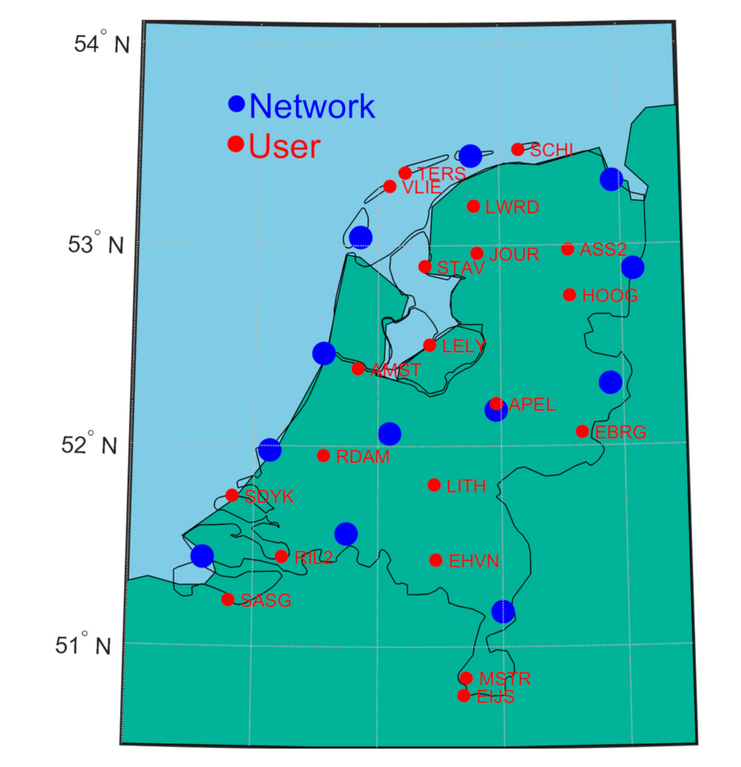
The Netherlands CORS network maintained by Kadaster is composed of 38 permanent stations, among which 12 stations are chosen as the reference to provide the satellite clock and phase bias corrections, and the average baseline length is about 100 km. Another 21 stations within or at the edge of the network are considered as the user locations to validate the solutions of the multi-GNSS PPP-RTK. The locations of the reference and user stations can be seen in Figure 1.
Table 1 summarizes the configurations of data processing. Precise a priori positions of the reference stations are applied in the data processing, and, at the network stations, the multi-GNSS data are processed in position-fixed mode, while, at the user stations, both kinematic and static positioning experiments are carried out. Precise multi-GNSS satellite orbits are assumed to be known and provided by the Center for Orbit Determination in Europe (CODE), which is contributed as a global analysis center to the IGS. A sample rate of 30 s is applied to balance between the change of receiver–satellite geometry and computational burden. An elevation cutoff angle of is set since satellites at low elevation angles are easily affected by many error sources, e.g., larger ionospheric and tropospheric delays due to the longer distance of passing through the atmosphere, and severe multipath in urban areas. All these errors may lead to a low signal-to-noise ratio and finally increase the measurement noise, which is why we apply the elevation-dependent weighting strategy.
The forward Kalman filter is implemented in the data processing, which means that this procedure can be easily applied in the real-time case as long as the precise real-time orbits are provided. Typically, the standard deviation of carrier-phase noise is less than 1 mm in the case of high carrier-to-noise-power-density ratio, and the code measurements are empirically weighted at least 100 times lower than the carrier phase due to their high noise. Therefore, taking into account the quality of the geodetic receivers, the standard deviation of the phase and code observables are set to 0.005 m and 0.5 m, respectively. We simply consider that the satellite and receiver clock offsets are unlinked in time, as well as the ionospheric delay, due to their properties of high temporal variations. The tropospheric delay, on the contrary, is highly constrained by a spectral density of because of its characterization of stability. Both satellite and receiver phase biases and ambiguities are considered as constant values. As mentioned before, only the ambiguities of GPS, Galileo, and BDS can be fixed to integers, while the GLONASS ambiguities are always kept as float values. The partial integer ambiguity resolution of LAMBDA is implemented in the data processing, which means that only a subset of ambiguities are fixed to integer values such that a user-defined success rate criterion, 0.999 in this study, is met, rather than fixing all ambiguities [59,60]. The positioning solutions with partial ambiguity resolution have the advantage of short convergence time since a long time might be needed to achieve a full ambiguity resolution.
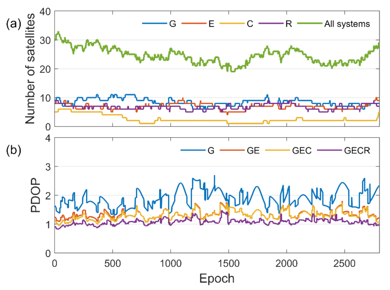
Figure 2 presents the number of satellites and position dilution of precision (PDOP) values at station APEL which is located at the center of the network. Since this is a local network, the number of the observed satellites would be more or less uniform in different stations. It can be seen that BDS does not have too many satellites observed because the receivers equipped in the network can only track one frequency of BDS-3 satellites and, therefore, only BDS-2 satellites are involved in the data processing.
A significant improvement in PDOP values can be seen at the bottom of Figure 2 from GPS alone to GPS + Galileo due to the increased number of observed satellites. However, the PDOPs are not distinguishable for GE and GEC after the 600th epoch because the number of observed BDS-2 satellites is not large enough to improve the geometry of GE. In addition, the improvement of the PDOP is marginal if one takes into account the contribution of GLONASS satellites since the geometry of GEC (or GE) is already good enough.
3.1. Kinematic Positioning Accuracy
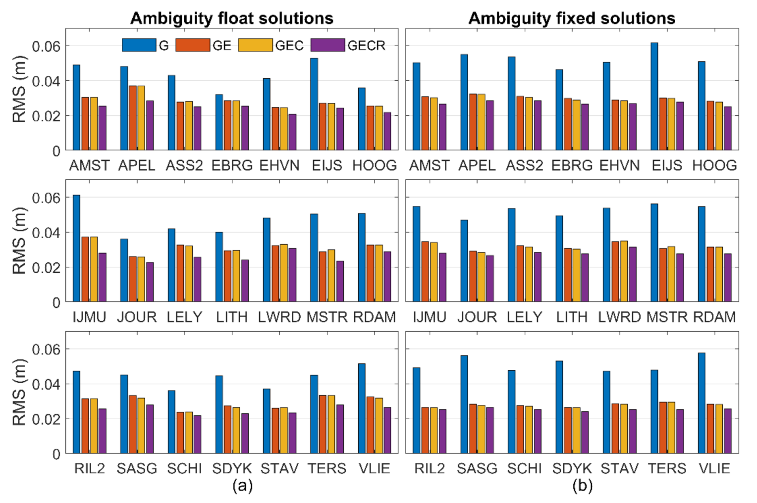
The data of 21 user stations are processed in kinematic mode without any constraints in the positioning parameters between epochs. Note that the user stations are stationary so that the accurate coordinates can be used for assessing the performances of the kinematic positioning. The positioning accuracy of the three-dimensional (3D) root-mean-square (RMS) errors are shown in Figure 3 in which the left column contains the ambiguity float solutions while the right column contains ambiguity fixed solutions. Note that the RMS statistics are calculated from the fourth hour to the end, during which positioning solutions are already fully converged. The accuracy improvements can be seen from GPS alone to GE for both ambiguity float and fixed solutions due to the strengthened geometry, and it is reasonable to see the similar performances achieved by GE and GEC due to the limited number of BDS satellites. There is no doubt that GECR has the most accurate positioning solutions as compared to other scenarios. However, the advantage of using GLONASS is insignificant for the ambiguity fixed solutions because, on the one hand, the geometry of GE/GEC is already strong enough; on the other hand, the float GLONASS solutions restrict the further improvement might be obtained by fixing GLONASS ambiguities.
One can see the abnormal behavior that the accuracies of the ambiguity fixed solutions of some stations in the GPS alone case are worse than those of the corresponding ambiguity float solutions. This is due to the incorrect integer ambiguity estimation, which may result in large positioning errors [61]. It is worthwhile to note that the wrong fixing is just an occasional issue that may be caused by many reasons, e.g., inaccurate corrections, data quality, and model errors. This might be caused by the drawback of LAMBDA which relies on the variance–covariance matrix of the estimations. Therefore, one may choose another integer ambiguity resolution method, e.g., precise and fast method of ambiguity resolution (PREFMAR), which can reliably fix the ambiguities without the information of variance matrix. However, this phenomenon does not exist in the combined systems which have more robust ambiguity fixed solutions. This is because both model strength and model errors are crucial for successful integer ambiguity resolution [62], yet the success rate criterion can only ensure a certain level of underlying model strength. As for the other factor model errors, obviously, they could severely impact the ambiguity estimation when the satellite–receiver geometry is not strong enough as the GPS alone case such that the integer ambiguities cannot be fixed correctly.
One can see in Figure 1 that most of the user stations are inside the network; however, there are still some stations on the edge of the network (e.g., SCHI, TERS, VLIE, and SDYK) or even outside the network (e.g., MSTR, EIJS, and SASG). As can be seen in Figure 3, the performances are not distinguishable between the seven specially located stations mentioned above and other inside network stations. This is because the PPP-RTK model is able to work well in the regional area and, thus, a global network is not necessary for generating the corresponding corrections. Furthermore, although some user stations are located outside, the distances are not far from the network. In such a case, all these stations are analyzed together as described below.
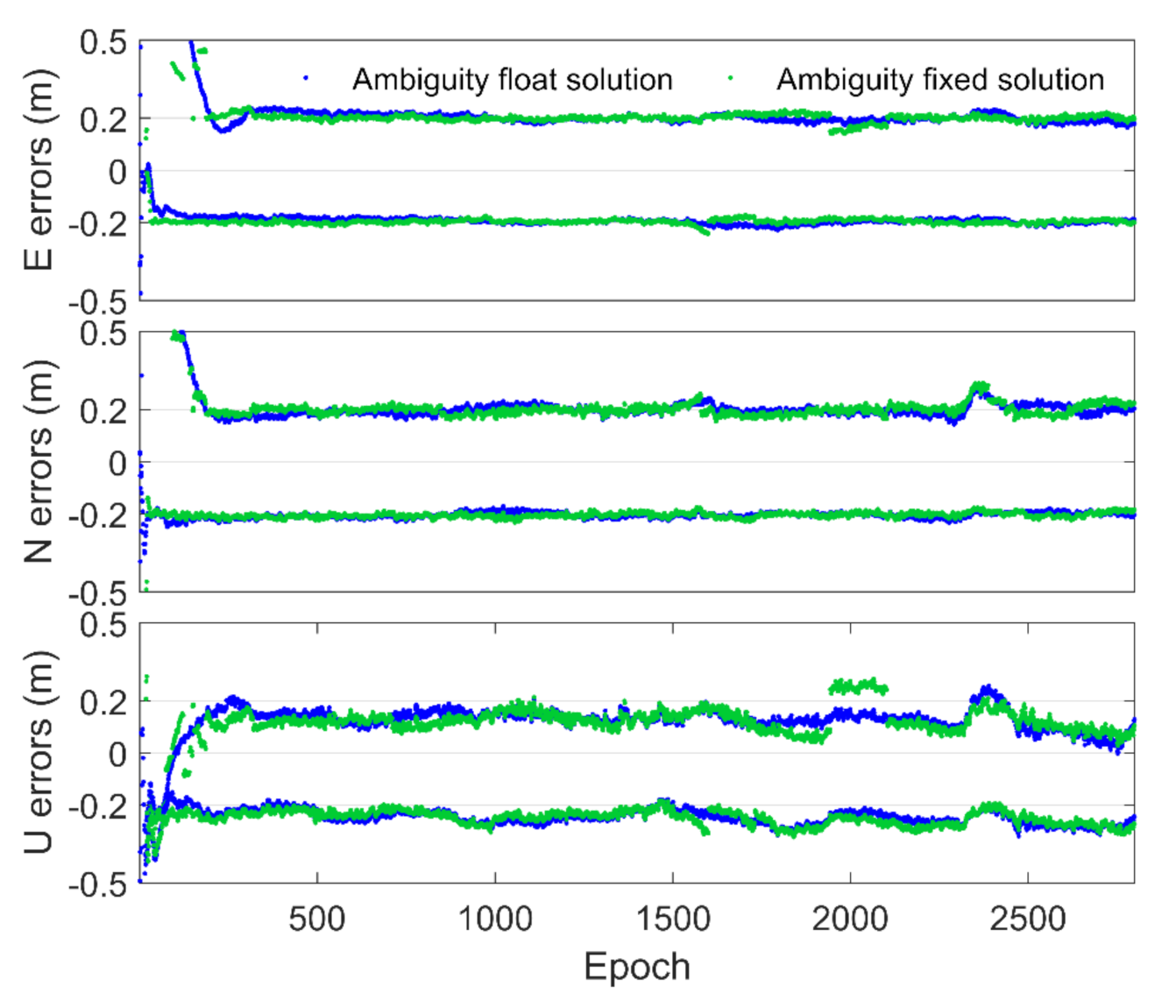
An example of the positioning solutions affected by wrongly fixed integer ambiguities is shown in Figure 4. The station HOOG is selected due to the greatest accuracy degradation of the ambiguity fixed solutions caused by the wrong fixing. One can see that unexpected U errors occur within the period of the 1700th to 2200th epoch in the GPS alone case; meanwhile, such errors disappear in the GPS + Galileo combination. It is obvious that the up component is mainly influenced, possibly due to the fact that the geometry of the vertical direction is not as good as that of the horizontal component.
Table 2 presents the average RMSs of the 3D and horizontal component of different combined systems. Except for GPS alone case for which the ambiguity fixed solutions are influenced by the wrong fixing problem, the ambiguity float and fixed solution performances of the remaining three combinations are almost the same. This is because, as can be seen in Figure 5, describing the gain in 3D precision which is the comparison of the ambiguity float precision and the ambiguity fixed precision, the contribution of fixing ambiguities on positions is insignificant after a long processing time, e.g., 500 epochs. This indicates that, theoretically, the ambiguity float solutions and the ambiguity fixed solutions can achieve the same positioning accuracy level after convergence. As for the GPS alone case, the deterioration of accuracy of the ambiguity fixed solution in the horizontal component is less than that of the 3D component thanks to the stronger geometry in the horizontal direction.
A large improvement in 3D ambiguity float solutions of more than 30% can be seen from G with 4.46 cm to GE/GEC with 2.99 cm/2.98 cm, and this is even more significant for the horizontal component with an improvement of 48%. This is consistent with the improved PDOP values in Figure 2 showing that multi-GNSS models are always stronger than GPS alone. It holds true even after convergence because of the large number of observed satellites. On the other hand, the contribution of additional GLONASS to ambiguity float positioning accuracy is insignificant when comparing GE/GEC and GECR, for which the improvement in 3D is 15%, and that in the horizontal component is 17%. Therefore, users of kinematic positioning may consider abandoning BDS in Western Europe if the receiver can only track BDS-2 satellites because GE can achieve almost the same performance as GEC. In addition, users may also exclude one or two systems to reduce the computational burden and complexity in the data processing since a stronger model results in less improvement when additional systems are introduced to the model.
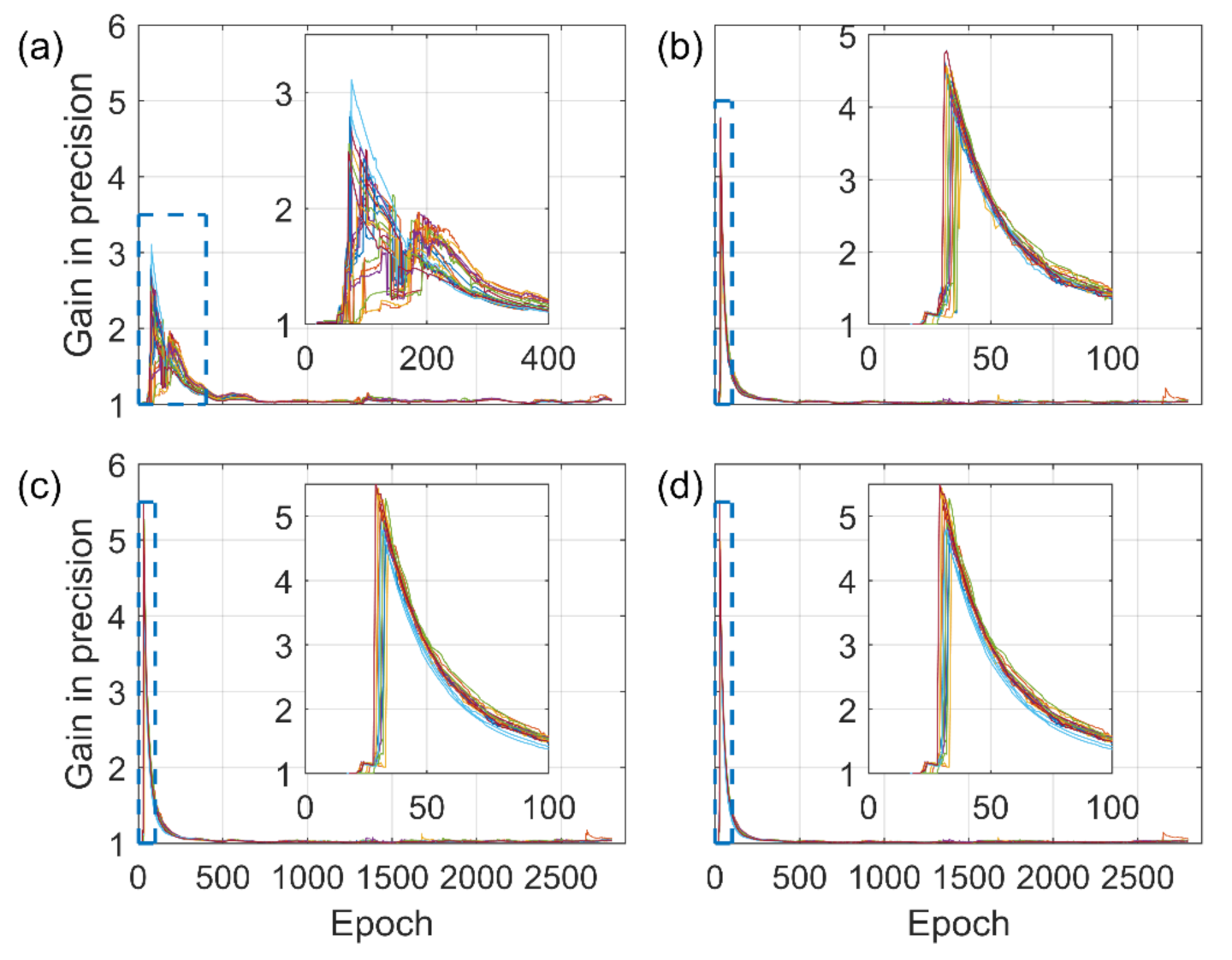
It can be seen in Figure 5 that the advantages of fixing ambiguities are not obvious after convergence when the ambiguity float model is already strong enough. However, these advantages appeared at the beginning of data processing, which can be clearly seen in the small windows of the subfigures. The values of gain in precision are 1 during the first dozens of epochs since no ambiguities are fixed due to the weak model strength; thus, for these epochs, the ambiguity fixed solutions are actually equivalent to the ambiguity float solutions. Then, the gain in precision rises since more ambiguities are getting fixed, and it drops after reaching a peak because the ambiguity float model is getting stronger with the accumulation of observations. For more information about how the fixed ambiguities contribute to the positioning precision, one can refer to [63,64].
One may have noticed that U curves appear around the 170th epoch for the GPS alone case. This might be because of the rise of new satellites which enhance the geometry of the ambiguity float solutions, while they do not contribute to the ambiguity fixed solutions because their ambiguities cannot be fixed immediately. Although, in Figure 5, each line represents one user station, the gain in precision of GPS + Galileo reaches a maximum value of 4.8, which is larger than GPS alone case with 3.1. Moreover, the time to achieve the maximum gain value decreases from an average of 70 epochs of GPS alone to 33 epochs of GPS + Galileo. The patterns of gain in precision of GEC are similar to those of GE, except for the insignificant improvements in maximum value with 5.5 and the average time to achieve maximum gain with 31 epochs. Since we do not fix the GLONASS ambiguities, the gain in precision of GECR is exactly the same as that of GEC.
Both improved maximum value and reduced time to achieve maximum gain indicate that the ambiguity fixed solutions of the combined systems would have shorter convergence times. Such improvements, although not evident, can even be seen when comparing GEC and GE. One may have seen this phenomenon in Figure 4 that ambiguity float and fixed positioning errors of GPS + Galileo can reduce to a certain accuracy level faster than those of GPS alone. Since the convergence time is another interest for users applying surveying and geodetic applications, we investigate the performances in terms of the convergence time of multi-GNSS PPP-RTK in the sections below.
3.2. Convergence Time of the Kinematic Positioning Mode
In order to obtain as many convergence times as possible to quantify the potential benefits offered by multi-GNSS PPP-RTK, the data processing was re-initialized for each user station at each integer hour from 0 h to 21 h, which means that, for each user station, we could have 22 convergence time solutions. The criterion for convergence was the last time the positioning errors, e.g., 3D, horizontal, and up components, decreased to a 10 cm level.
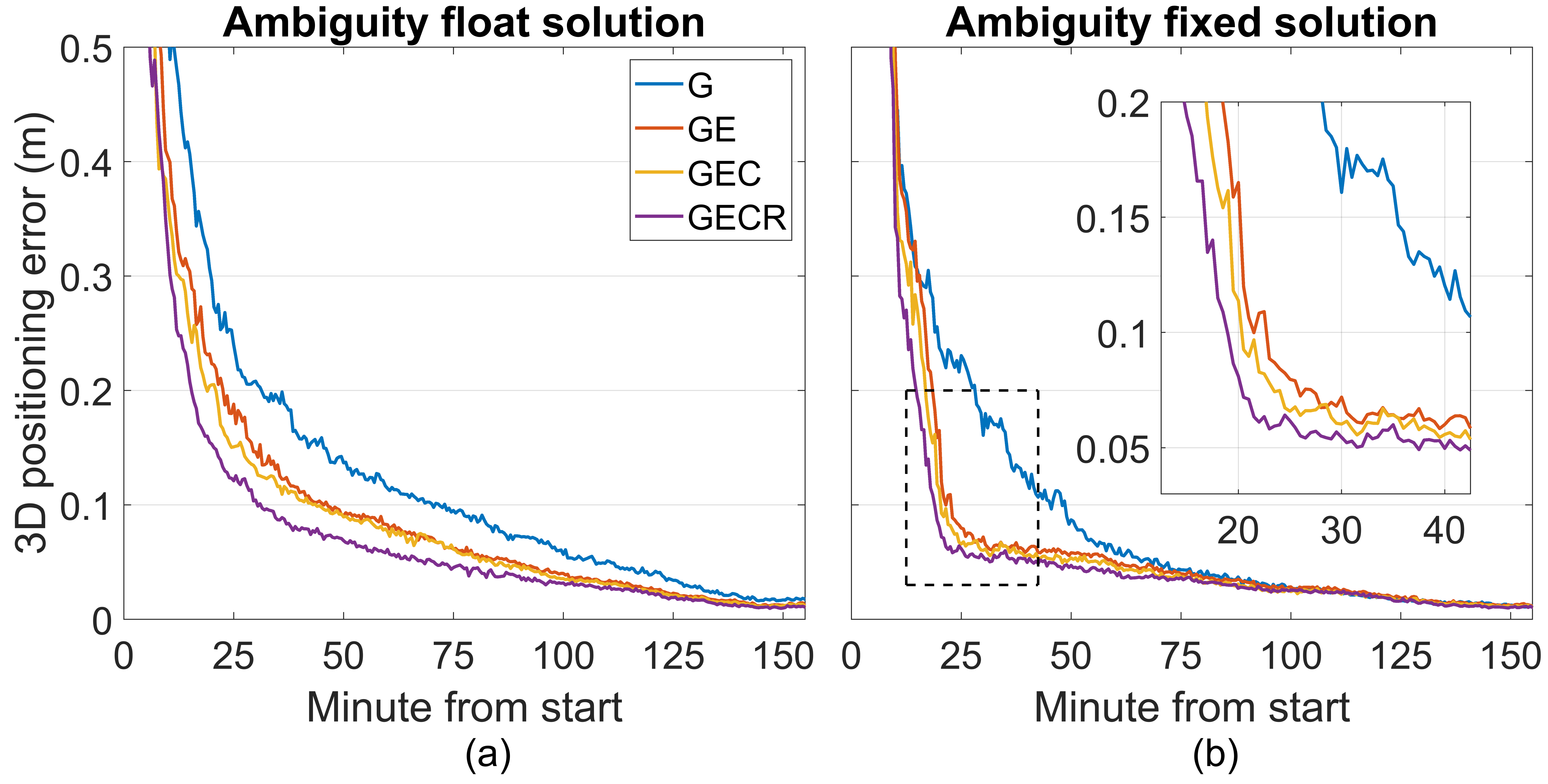
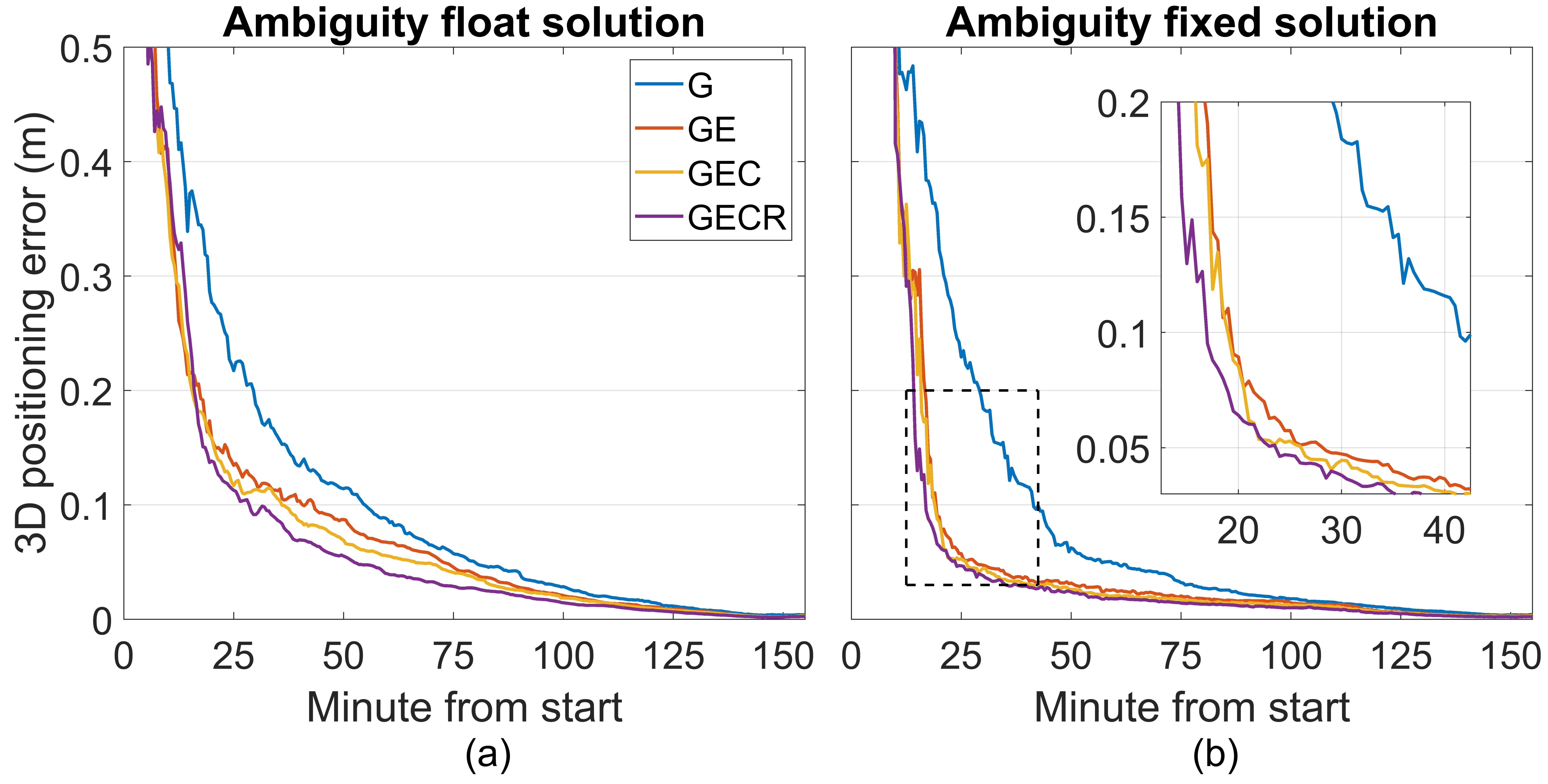
Figure 6 illustrates the overall performances of the ambiguity float and fixed solutions with 90% probability, which means that 90% of the positioning errors are smaller than those shown in the figure. The reason for not taking into account all convergence solutions is to avoid the unexpected model errors which might cause unusual positioning behavior in data processing. One can see that, unlike the time series of the ambiguity float positioning errors in the shape of a curve, the ambiguity fixed errors decrease rapidly once most of the ambiguities are successfully fixed, except for the GPS alone case due to the wrong fixing problem. The ambiguity fixed solutions of GPS alone are mainly affected within the period of the 1700th to 2200th epochs, as can be seen in the example of the user station HOOG in Figure 4. This causes the unusual behavior of the GPS ambiguity fixed positioning errors.
As for the combinations GE, GEC, and GECR, on the contrary, the ambiguity fixed positioning errors are significantly decreased within the 15th to 20th min, which is consistent with the peak values of the gain in precision shown in Figure 5 (30th to 40th epochs). This demonstrates that successful integer ambiguity resolution is the key to fast and high-accuracy GNSS positioning. Additionally, it is worth noting that, after a long convergence time, the ambiguity float solutions can achieve a similar accuracy level to the ambiguity fixed solutions. This also holds true for the multi-GNSS case and GPS alone case, although the latter suffers from the wrong fixing problem. Therefore, we can conclude that one of the purposes of fixing ambiguities is identical to that of the multi-GNSS, i.e., to reduce the convergence time.
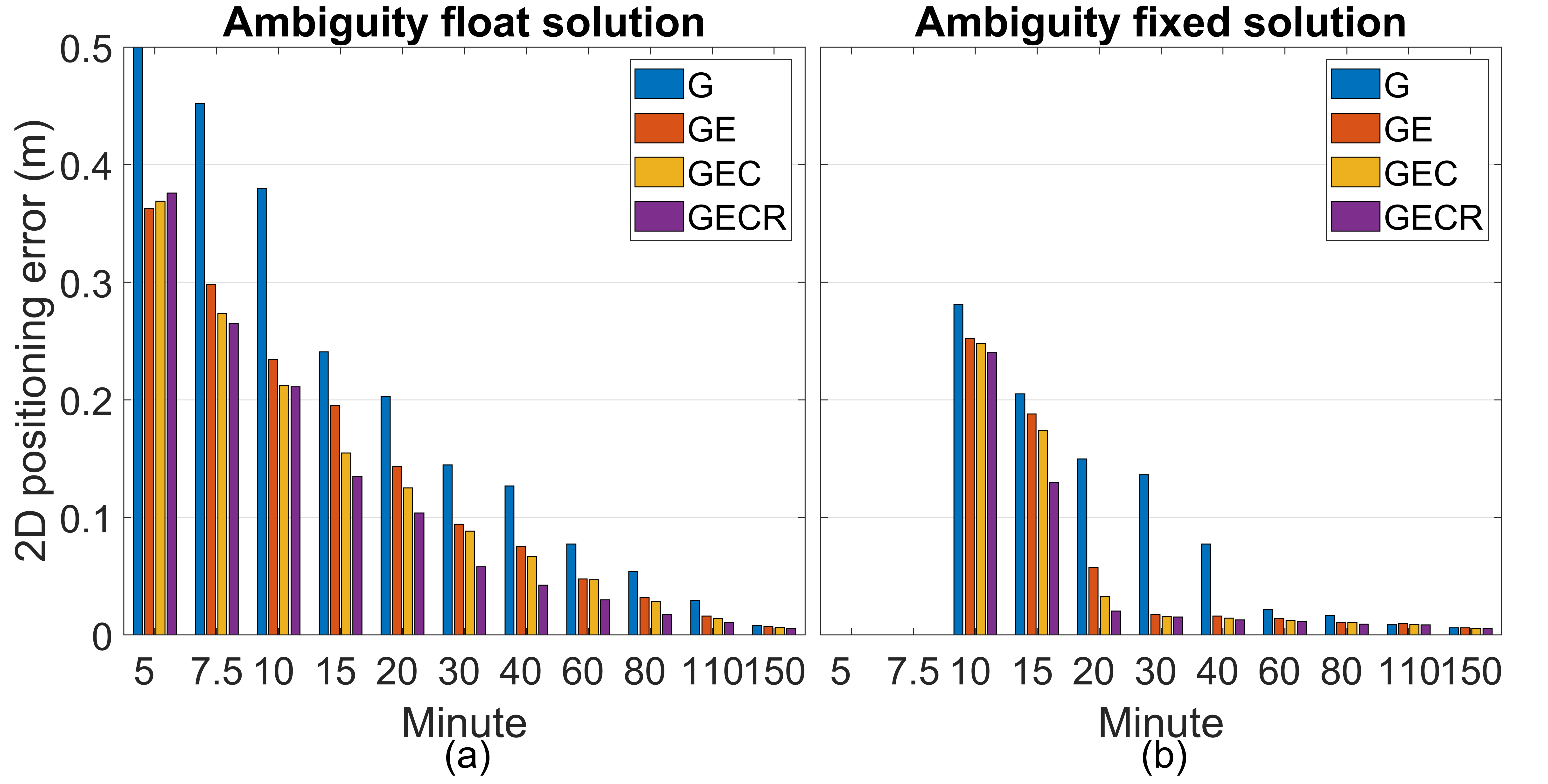
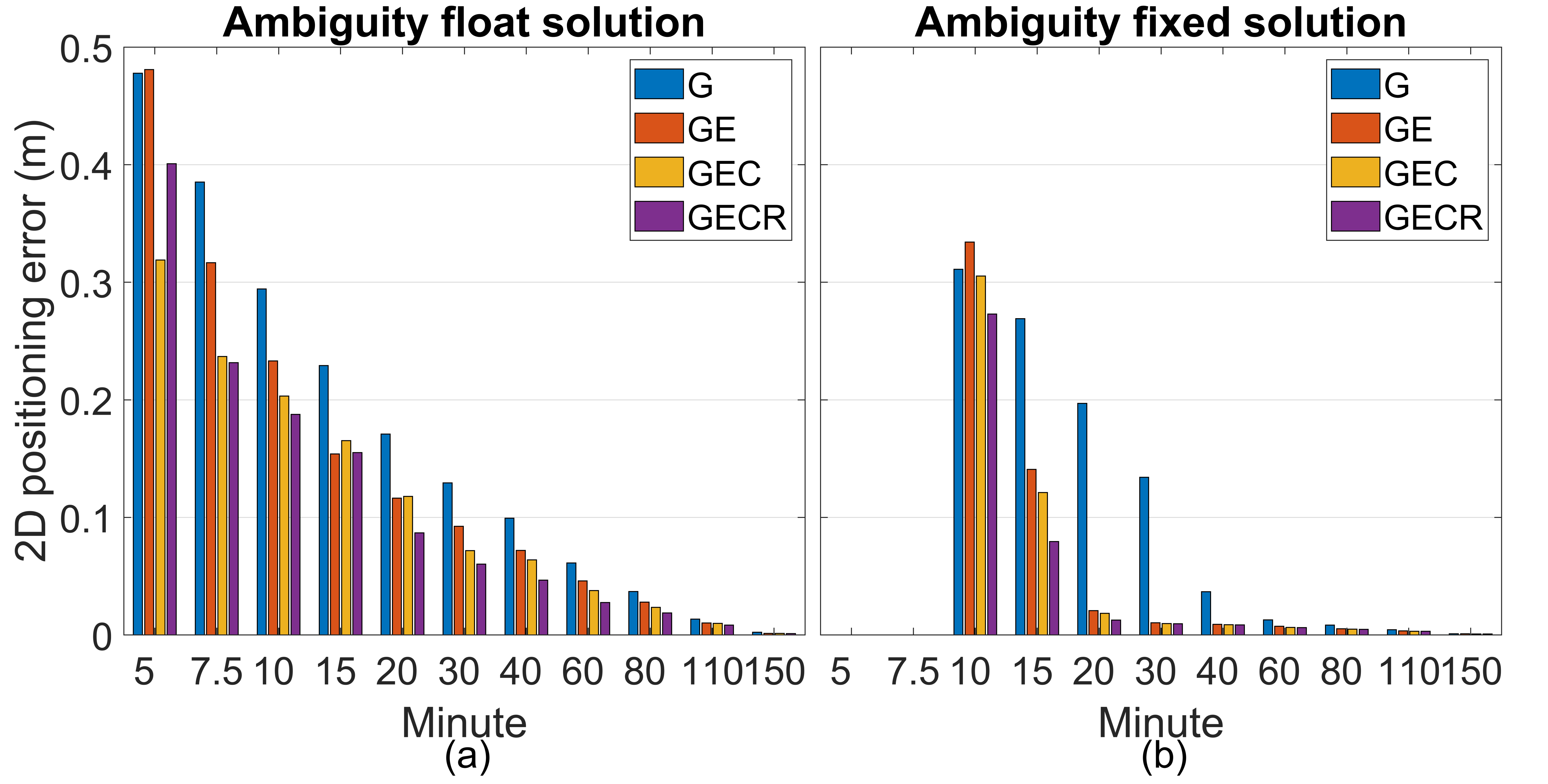
The overall horizontal ambiguity float and fixed positioning errors at specific minutes are presented in Figure 7. Since the first ambiguity is fixed no earlier than the 15th epoch for all combined GNSS cases, the ambiguity fixed solutions are absent at the fifth and 7.5th min. Users could use the ambiguity float solutions at the beginning of data processing when the ambiguity fixed solutions are not available in practical applications. The large improvements in ambiguity fixed GE, GEC, and GECR solutions can be confidently seen from the 15th to 20th min during which the gain in precision of most user stations achieves the maximum value. As for the GPS alone case, such a significant improvement in ambiguity fixed solution appeared within the 40th to 60th min, which is identical to the same period when the gain in precision of GPS alone reached the peak height (Figure 5).
Figure 7 shows that, at the 150th min, i.e., 2.5 h, the ambiguity float and fixed positioning solutions of all cases arrive the same accuracy level. Before that moment, both ambiguity float and fixed positioning solutions benefited from the extra GNSS system, although not too many BDS-2 satellites could be observed. However, the advantage of multi-GNSS is marginal as the positioning models are getting stronger when new constellations are added.
Table 3 presents a summary of the convergence times in different GNSS combinations. It can be seen that the ambiguity fixed solutions can achieve similar performances to those of multi-system ambiguity float solutions. For instance, the ambiguity fixed convergence time of GPS alone in 3D is 46.5 min, which is approximate to the ambiguity float of GE with 45.5 min and GEC with 43.5 min. Although, for the horizontal component, the ambiguity fixed convergence time of GPS alone is longer than the ambiguity float of GE/GEC, the ambiguity fixed GE is better than the ambiguity float GEC/GECR for both 3D and horizontal component.
One can see the significant improvements from GPS alone to GPS + Galileo, but not from GE to GEC or from GEC to GECR. This is because the geometry of GE/GEC is already good enough for the ambiguity float solutions as compared to GPS alone (seen in Figure 2 the PDOP values), and the float GLONASS ambiguities have a further shortened convergence time for GREC ambiguity fixed solutions.
3.3. Convergence Time of the Static Positioning Mode
The convergence time is also crucial for static positioning mode in geodetic applications, for instance, the stop-and-go surveying technique for which the coordinates of the receiver are only of interest when it is stationary. Applying multi-GNSS observations and/or fixing ambiguities could improve the efficiency and productivity of this technology because the receiver continues to function while it is being moved from one stationary setup to the next.
As can be seen in Figure 8, showing the 3D positioning errors of different combinations, only the GPS alone case has a relatively large improvement when compared to the corresponding kinematic positioning errors of Figure 6. This is because the underlying models of the combined cases are already strong enough and, therefore, less sensitive to the positions regarded as constant values. The improved GPS alone performance also indicates that the static positioning mode with a stronger model is less likely to suffer from the wrong fixing problem.
The static positioning errors are closer to 0 after a certain convergence time as compared to those of the kinematic positioning solutions. This phenomenon is evident for the ambiguity fixed solutions of 3D in Figure 8 and the horizontal component in Figure 9, showing the horizontal positioning errors at specific minutes. This indicates that the static positioning with the integer ambiguity resolution has the potential benefits to achieve a sub-centimeter error level within a short period. As can be seen the ambiguity fixed solutions in Figure 9, the combined systems GE/GEC/GECR are very accurate at the 30th min, and GPS alone achieves a similar accuracy level at the 60th min. On the other hand, for the kinematic positioning solutions shown in Figure 7, it takes 80 and 110 min for the combined systems and GPS alone, respectively.
Table 4 contains not only the convergence times to achieve the sub-decimeter 10 cm accuracy level, but also those to achieve sub-centimeter 1 cm accuracy. As already discussed before, only the GPS alone case sees substantial improvements in the 10 cm criterion compared to Table 3, showing the kinematic positioning solutions, e.g., from the 3D kinematic ambiguity float with 70 min to that of the static ambiguity float with 53 min.
The overall convergence time performances of the static positioning are similar to those of the kinematic solutions. Furthermore, it is worth noting that the integer ambiguity resolution has a major contribution to sub-centimeter level accuracy, as presented in Table 4, where the numbers in brackets are the convergence criterion of 1 cm. Due to the high correlation between ambiguities and the horizontal component, the shortened convergence times to the sub-centimeter level of the horizontal component are more obvious than those of the 3D positioning solutions. In general, one could expect around 1 h of observation length to obtain 1 cm positioning accuracy for GPS alone and 0.5 h for the combined systems GE/GEC/GECR.
4. Discussions
Positioning results have shown that the ambiguity fixed solutions of GPS alone occasionally suffer from wrong fixing problem. This might be due to the drawback of LAMBDA which relies on the covariance matrix of ambiguity, and in the GPS-only case, the covariance matrix may be over-optimistic for describing the actual uncertainty of the ambiguity. One way to correctly fix ambiguities is, as demonstrated in this contribution, using combined systems GE/GEC/GECR. Another way is to choose another integer ambiguity resolution method which may reliably fix the ambiguities without the information of variance matrix. Besides, using atmospheric augmentation is also a method to strengthen the GPS-alone model, and another choice is applying the ratio test with fixed failure rate.
As the contributions brought from the additional constellations are only marginal, users may consider the computational burden and complexity by involving extra systems since exclude one or two systems to simplify the data processing because the stronger the model is, the less the improvement is when additional systems are introduced in the model. On the other hand, the RMSs of the ambiguity fixed solutions are close to those of the ambiguity float solutions because the gain in precision of fixing ambiguities is limited after convergence.
5. Conclusions
In this contribution, the performances of the multi-GNSS PPP-RTK are assessed since both multi constellations and integer ambiguity resolution bring with them improvements in productivity and efficiency. An undifferenced and uncombined PPP-RTK model is constructed, and the CORS network of the Netherlands containing 12 reference stations and 21 user stations is used to verify the positioning accuracy and convergence time of the multi-GNSS PPP-RTK model.
In the positioning experiments, the accuracy of ambiguity float and fixed solutions is improved as extra constellation being added into data processing because the geometry is strengthened. However, such improvements are marginal when more GNSS systems are included, for example, around 30% improvement of the 3D ambiguity float solutions can be seen from G with 4.32 cm to GE with 2.99 cm; however, only 15% from GEC with 2.98 cm to GECR with 2.52 cm.
As for the convergence time experiments, the ambiguity fixed errors of the combined systems are significantly decreased within the period 15th to 20th minute during which the gain in precision of most user stations reaches to the maximum value. The overall convergence time performances of kinematic and static mode are similar to those of the positioning experiments, which are a significant improvement from G to GE/GEC and insignificant from GE/GEC to GECR. The contribution of fixing ambiguities on reducing the convergence times is seen for all cases, including GPS alone affected by wrong fixing. Besides, the results also indicate that integer ambiguity resolution is still necessary for sub-centimeter level accuracy for the multi-GNSS case.
Author Contributions
Methodology, H.M. and S.V.; software, H.M. and D.P.; validation, Q.Z. and X.L.; investigation, H.M.; writing—original draft preparation, H.M.; writing—review and editing, Q.Z., S.V., X.L., and D.P.; visualization, H.M.; supervision, S.V. and X.L. All authors read and agreed to the published version of the manuscript.
Funding
The first and fourth authors received funding from the European Union’s Horizon 2020 research and innovation program under the Marie-Sklodowska Grant No 722023. This research was also partially supported by National Natural Science Foundation of China (Grant No 41774035).
Acknowledgments
The authors would like to thank Kadaster for maintaining the Netherlands GNSS network. The authors are thankful to the Center for Orbit Determination in Europe for providing the precise satellite orbits.
Conflicts of Interest
The authors declare no conflict of interest.
References
- Langley, R.B.; Teunissen, P.J.; Montenbruck, O. Introduction to GNSS. In Springer Handbook of Global Navigation Satellite Systems, 1st ed.; Teunissen, P., Montenbruck, O., Eds.; Springer: Berlin/Heidelberg, Germany, 2017; pp. 3–23. [Google Scholar] [CrossRef]
- Montenbruck, O.; Steigenberger, P.; Prange, L.; Deng, Z.; Zhao, Q.; Perosanz, F.; Schmid, R. The Multi-GNSS Experiment (MGEX) of the International GNSS Service (IGS)–achievements, prospects and challenges. Adv. Space Res. 2017, 59, 1671–1697. [Google Scholar] [CrossRef]
- Yang, Y.; Li, J.; Xu, J.; Tang, J.; Guo, H.; He, H. Contribution of the compass satellite navigation system to global PNT users. Chin. Sci. Bull. 2011, 56, 2813–2824. [Google Scholar] [CrossRef] [Green Version]
- Steigenberger, P.; Hugentobler, U.; Loyer, S.; Perosanz, F.; Prange, L.; Dach, R.; Montenbruck, O. Galileo orbit and clock quality of the IGS Multi-GNSS Experiment. Adv. Space Res. 2015, 55, 269–281. [Google Scholar] [CrossRef]
- Odolinski, R.; Teunissen, P.J.; Odijk, D. Combined bds, Galileo, qzss and gps single-frequency rtk. Gps Solut. 2015, 19, 151–163. [Google Scholar] [CrossRef]
- Zumberge, J.F.; Heflin, M.B.; Jefferson, D.C.; Watkins, M.M.; Webb, F.H. Precise point positioning for the efficient and robust analysis of GPS data from large networks. J. Geophys. Res. Sol. Earth 1997, 102, 5005–5017. [Google Scholar] [CrossRef] [Green Version]
- Kouba, J.; Héroux, P. Precise point positioning using IGS orbit and clock products. Gps Solut. 2001, 5, 12–28. [Google Scholar] [CrossRef]
- Cai, C.; Gao, Y. Modeling and assessment of combined GPS/GLONASS precise point positioning. Gps Solut. 2013, 17, 223–236. [Google Scholar] [CrossRef]
- Zhao, Q.; Wang, C.; Guo, J.; Liu, X. Assessment of the Contribution of BeiDou GEO, IGSO, and MEO Satellites to PPP in Asia—Pacific Region. Sensors 2015, 15, 29970–29983. [Google Scholar] [CrossRef] [Green Version]
- Li, X.; Ge, M.; Dai, X.; Ren, X.; Fritsche, M.; Wickert, J.; Schuh, H. Accuracy and reliability of multi-GNSS real-time precise positioning: GPS, GLONASS, BeiDou, and Galileo. J. Geod. 2015, 89, 607–635. [Google Scholar] [CrossRef]
- Liu, T.; Yuan, Y.; Zhang, B.; Wang, N.; Tan, B.; Chen, Y. Multi-GNSS precise point positioning (MGPPP) using raw observations. J. Geod. 2017, 91, 253–268. [Google Scholar] [CrossRef]
- Pan, Z.; Chai, H.; Kong, Y. Integrating multi-GNSS to improve the performance of precise point positioning. Adv. Space Res. 2017, 60, 2596–2606. [Google Scholar] [CrossRef]
- Aggrey, J.; Bisnath, S. Performance analysis of atmospheric constrained uncombined multi-GNSS PPP. In Proceedings of the ION GNSS+, Institute of Navigation, Portland, OR, USA, 18–23 September 2017; pp. 15–20. [Google Scholar]
- Psychas, D.; Bruno, J.; Massarweh, L.; Darugna, F. Towards Sub-meter Positioning using Android Raw GNSS Measurements. In Proceedings of the ION GNSS+, Institute of Navigation, Miami, FL, USA, 16–20 September 2019; pp. 3917–3931. [Google Scholar]
- Teunissen, P.J. Carrier phase integer ambiguity resolution. In Springer Handbook of Global Navigation Satellite Systems, 1st ed.; Teunissen, P., Montenbruck, O., Eds.; Springer: Berlin/Heidelberg, Germany, 2017; pp. 661–685. [Google Scholar] [CrossRef]
- Ge, M.; Gendt, G.; Rothacher, M.A.; Shi, C.; Liu, J. Resolution of GPS carrier-phase ambiguities in precise point positioning (PPP) with daily observations. J. Geod. 2008, 82, 389–399. [Google Scholar] [CrossRef]
- Qu, L.; Zhao, Q.; Guo, J.; Wang, G.; Guo, X.; Zhang, Q.; Luo, L. BDS/GNSS real-time kinematic precise point positioning with un-differenced ambiguity resolution. In Proceedings of the China Satellite Navigation Conference, China Satellite Navigation Office, Xi’an, China, 13–15 May 2015; Volume III, pp. 13–29. [Google Scholar] [CrossRef]
- Li, X.; Li, X.; Yuan, Y.; Zhang, K.; Zhang, X.; Wickert, J. Multi-GNSS phase delay estimation and PPP ambiguity resolution: GPS, BDS, GLONASS, Galileo. J. Geod. 2018, 92, 579–608. [Google Scholar] [CrossRef]
- Geng, J.; Chen, X.; Pan, Y.; Zhao, Q. A modified phase clock/bias model to improve PPP ambiguity resolution at Wuhan University. J. Geod. 2019, 93, 2053–2067. [Google Scholar] [CrossRef]
- Geng, J.; Li, X.; Zhao, Q.; Li, G. Inter-system PPP ambiguity resolution between GPS and BeiDou for rapid initialization. J. Geod. 2019, 93, 383–398. [Google Scholar] [CrossRef]
- Teunissen, P.J.; Odijk, D.; Zhang, B. PPP-RTK: Results of CORS network-based PPP with integer ambiguity resolution. J. Aeronaut. Astronaut. Aviat. Ser. A 2010, 42, 223–230. [Google Scholar] [CrossRef]
- Zhang, B.; Teunissen, P.J.; Odijk, D. A novel un-differenced PPP-RTK concept. J. Navig. 2011, 64, 180–191. [Google Scholar] [CrossRef] [Green Version]
- Verhagen, S.; Odijk, D.; Teunissen, P.J.; Huisman, L. Performance improvement with low-cost multi-GNSS receivers. In Proceedings of the ESA workshop on satellite navigation technologies and European workshop on GNSS signals and signal processing, ESA, Noordwijk, The Netherlands, 8–10 December 2010; pp. 1–8. [Google Scholar] [CrossRef] [Green Version]
- Odijk, D.; Zhang, B.; Teunissen, P.J. Multi-GNSS PPP and PPP-RTK: Some GPS+ BDS Results in Australia. In Proceedings of the China Satellite Navigation Conference, China Satellite Navigation Office, Xi’an, China, 13–15 May 2015; Volume II, pp. 613–623. [Google Scholar] [CrossRef]
- Khodabandeh, A.; Teunissen, P.J.G. PPP-RTK and inter-system biases: The ISB look-up table as a means to support multi-system PPP-RTK. J. Geod. 2016, 90, 837–851. [Google Scholar] [CrossRef] [Green Version]
- Liu, X.; Goode, M.; Tegedor, J.; Vigen, E.; Oerpen, O.; Strandli, R. Real-time multi-constellation precise point positioning with integer ambiguity resolution. In Proceedings of the International Association of Institutes of Navigation World Congress (IAIN), Prague, Czech Republic, 20–23 October 2015; pp. 1–7. [Google Scholar] [CrossRef]
- Verhagen, S.; Teunissen, P.J. Least-squaRes. estimation and Kalman filtering. In Springer Handbook of Global Navigation Satellite Systems, 1st ed.; Teunissen, P., Montenbruck, O., Eds.; Springer: Berlin/Heidelberg, Germany, 2017; pp. 639–660. [Google Scholar] [CrossRef]
- Teunissen, P.J. Least-squaRes. estimation of the integer GPS ambiguities. In Proceedings of the Invited Lecture, Section IV Theory and Methodology, IAG General Meeting, Beijing, China, 6–13 August 1993. [Google Scholar]
- Teunissen, P.J. The least-squaRes. ambiguity decorrelation adjustment: A method for fast GPS integer ambiguity estimation. J. Geod. 1995, 70, 65–82. [Google Scholar] [CrossRef]
- Bakuła, M. Precise Method of Ambiguity Initialization for Short Baselines with L1-L5 or E5-E5a GPS/GALILEO Data. Sensors 2020, 20, 4318. [Google Scholar] [CrossRef]
- Vollath, U.; Birnbach, S.; Landau, L.; FRAILE-ORDOÑEZ, J.M.; Martí-Neira, M. Analysis of Three-Carrier Ambiguity Resolution Technique for Precise Relative Positioning in GNSS-2. Navigation 1999, 46, 13–23. [Google Scholar] [CrossRef]
- Hatch, R.; Jung, J.; Enge, P.; Pervan, B. Civilian GPS: The benefits of three frequencies. Gps Solut. 2000, 3, 1–9. [Google Scholar] [CrossRef]
- Ruwisch, F.; Jain, A.; Schön, S. Characterisation of GNSS Carrier Phase Data on a Moving Zero-Baseline in Urban and Aerial Navigation. Sensors 2020, 20, 4046. [Google Scholar] [CrossRef]
- Krasuski, K.; Ciećko, A.; Bakuła, M.; Wierzbicki, D. New Strategy for Improving the Accuracy of Aircraft Positioning Based on GPS SPP Solution. Sensors 2020, 20, 4921. [Google Scholar] [CrossRef] [PubMed]
- Krasuski, K.; Wierzbicki, D.; Jafernik, H. Utilization PPP method in aircraft positioning in post-processing mode. Aircr. Eng. Aerosp. Technol. 2018, 90, 202–209. [Google Scholar] [CrossRef]
- Alkan, R.M.; Öcalan, T. Usability of the GPS precise point positioning technique in marine applications. J. Navig. 2013, 66, 579–588. [Google Scholar] [CrossRef] [Green Version]
- El-Diasty, M. Integrity analysis of real-time PPP technique with Igs-Rts service for maritime navigation. Int. Arch. Photogramm. Remote Sens. Spat. Inf. Sci. 2017, 42, 61–66. [Google Scholar] [CrossRef] [Green Version]
- Liu, Y.; Liu, F.; Gao, Y.; Zhao, L. Implementation and analysis of tightly coupled global navigation satellite system precise point positioning/inertial navigation system (GNSS PPP/INS) with insufficient satellites for land vehicle navigation. Sensors 2018, 18, 4305. [Google Scholar] [CrossRef] [Green Version]
- Krasuski, K.; Ciećko, A.; Grunwald, G.; Wierzbicki, D. Assessment of velocity accuracy of aircraft in the dynamic tests using GNSS sensors. Facta Univ. Ser. Mech. Eng. 2020, 18, 301–313. [Google Scholar] [CrossRef]
- Bakuła, M.; Przestrzelski, P.; Kaźmierczak, R. Reliable technology of centimeter GPS/GLONASS surveying in forest environments. IEEE Trans. Geosci. Remote Sens. 2014, 53, 1029–1038. [Google Scholar] [CrossRef]
- Hinüber, E.L.; Reimer, C.; Schneider, T.; Stock, M. INS/GNSS integration for aerobatic flight applications and aircraft motion surveying. Sensors 2017, 17, 941. [Google Scholar] [CrossRef] [PubMed] [Green Version]
- Bakuła, M. An approach to reliable rapid static GNSS surveying. Surv. Rev. 2012, 44, 265–271. [Google Scholar] [CrossRef]
- Bruni, S.; Rebischung, P.; Zerbini, S.; Altamimi, Z.; Errico, M.; Santi, E. Assessment of the possible contribution of space ties on-board GNSS satellites to the terrestrial reference frame. J. Geod. 2018, 92, 383–399. [Google Scholar] [CrossRef]
- Zanutta, A.; Negusini, M.; Vittuari, L.; Cianfarra, P.; Salvini, F.; Mancini, F.; Capra, A. Monitoring geodynamic activity in the Victoria Land, East Antarctica: Evidence from GNSS measurements. J. Geodyn. 2017, 110, 31–42. [Google Scholar] [CrossRef]
- Uradziński, M.; Bakuła, M. Assessment of static positioning accuracy using low-cost smartphone GPS devices for geodetic survey points’ determination and monitoring. Appl. Sci. 2020, 10, 5308. [Google Scholar] [CrossRef]
- Bakuła, M. Study of reliable rapid and ultrarapid static GNSS surveying for determination of the coordinates of control points in obstructed conditions. J. Surv. Eng. 2013, 139, 188–193. [Google Scholar] [CrossRef]
- Wanninger, L. Carrier-phase inter-frequency biases of GLONASS receivers. J. Geod. 2012, 86, 139–148. [Google Scholar] [CrossRef] [Green Version]
- Banville, S.; Collins, P.; Lahaye, F. GLONASS ambiguity resolution of mixed receiver types without external calibration. Gps Solut. 2013, 17, 275–282. [Google Scholar] [CrossRef]
- Teunissen, P.J.G.; Khodabandeh, A. GLONASS ambiguity resolution. Gps Solut. 2019, 23, 101–116. [Google Scholar] [CrossRef] [Green Version]
- Teunissen, P. Zero Order Design: Generalized Inverses, Adjustment, the Datum Problem and S-Transformations, 1st ed.; Springer: Berlin/Heidelberg, Germany, 1985; pp. 11–55. [Google Scholar]
- Odijk, D.; Zhang, B.; Khodabandeh, A.; Odolinski, R.; Teunissen, P.J. On the estimability of parameters in undifferenced, uncombined GN network and PPP-RTK user models by means of S-system theory. J. Geod. 2016, 90, 15–44. [Google Scholar] [CrossRef]
- Psychas, D.; Verhagen, S.; Liu, X.; Memarzadeh, Y.; Visser, H. Assessment of ionospheric corrections for PPP-RTK using regional ionosphere modelling. Meas. Sci. Technol. 2018, 30, 014001. [Google Scholar] [CrossRef] [Green Version]
- Psychas, D.; Verhagen, S. Real-Time PPP-RTK Performance Analysis Using Ionospheric Corrections from Multi-Scale Network Configurations. Sensors 2020, 20, 3012. [Google Scholar] [CrossRef] [PubMed]
- El-Mowafy, A.; Deo, M.; Kubo, N. Maintaining real-time precise point positioning during outages of orbit and clock corrections. Gps Solut. 2017, 21, 937–947. [Google Scholar] [CrossRef]
- Wang, K.; Khodabandeh, A.; Teunissen, P. A study on predicting network corrections in PPP-RTK processing. Adv. Space Res. 2017, 60, 1463–1477. [Google Scholar] [CrossRef] [Green Version]
- Khodabandeh, A.; Teunissen, P.J.G. Array-based satellite phase bias sensing: Theory and GPS/BeiDou/QZSS results. Meas. Sci. Technol. 2014, 25, 095801. [Google Scholar] [CrossRef] [Green Version]
- Henkel, P.; Psychas, D.; Günther, C.; Hugentobler, U. Estimation of satellite position, clock and phase bias corrections. J. Geod. 2018, 92, 1199–1217. [Google Scholar] [CrossRef]
- Odijk, D.; Teunissen, P.J. Characterization of between-receiver GPS-Galileo inter-system biases and their effect on mixed ambiguity resolution. Gps Solut. 2013, 17, 521–533. [Google Scholar] [CrossRef]
- Verhagen, S.; Teunissen, P.J.; van der Marel, H.; Li, B. GNSS ambiguity resolution: Which subset to fix. In Proceedings of the International Global Navigation Satellite Systems Society, IGNSS Symposium, University of New South Wales, Australia, 15–17 November 2011; pp. 1–15. [Google Scholar]
- Teunissen, P.; Verhagen, S. GNSS Carrier phase ambiguity resolution: Challenges and open problems. In Observing Our Changing Earth, 1st ed.; Sideris, M.G., Ed.; Springer: Berlin/Heidelberg, Germany, 2009; pp. 133–145. [Google Scholar] [CrossRef] [Green Version]
- Verhagen, S.; Li, B.; Teunissen, P.J. Ps-LAMBDA: Ambiguity success rate evaluation software for interferometric applications. Comput. Geosci. 2013, 54, 361–376. [Google Scholar] [CrossRef] [Green Version]
- Li, B.; Verhagen, S.; Teunissen, P.J. Robustness of GNSS integer ambiguity resolution in the presence of atmospheric biases. Gps Solut. 2014, 18, 283–296. [Google Scholar] [CrossRef]
- Teunissen, P.J. Success probability of integer GPS ambiguity rounding and bootstrapping. J. Geod. 1998, 72, 606–612. [Google Scholar] [CrossRef] [Green Version]
- Teunissen, P.J.G. The distribution of the GPS baseline in case of integer least-squaRes. ambiguity estimation. Artif. Satell. 1998, 33, 65–75. [Google Scholar]
Figure 1.
Global navigation satellite system (GNSS) network of the Netherlands, where blue points represent reference stations and red points are user stations.
Figure 1.
Global navigation satellite system (GNSS) network of the Netherlands, where blue points represent reference stations and red points are user stations.

Figure 2.
(a) Number of satellites and (b) position dilution of precision (PDOP) at station APEL.

Figure 3.
Three-dimensional (3D) positioning accuracy of the (a) ambiguity float solution and (b) ambiguity fixed solution.
Figure 3.
Three-dimensional (3D) positioning accuracy of the (a) ambiguity float solution and (b) ambiguity fixed solution.

Figure 4.
Time series of the ambiguity float and fixed solutions of station HOOG in the case of GPS alone and GPS + Galileo. The solutions of G and GE are shifted by +0.2 m and −0.2 m, respectively.
Figure 4.
Time series of the ambiguity float and fixed solutions of station HOOG in the case of GPS alone and GPS + Galileo. The solutions of G and GE are shifted by +0.2 m and −0.2 m, respectively.

Figure 5.
Gain in 3D precision of the four multi-GNSS combing cases with (a) GPS only, (b) GE, (c) GEC, and (d) GECR. Each line represents one user station.
Figure 5.
Gain in 3D precision of the four multi-GNSS combing cases with (a) GPS only, (b) GE, (c) GEC, and (d) GECR. Each line represents one user station.

Figure 6.
(a) The 3D ambiguity float positioning errors and (b) 3D ambiguity fixed positioning errors of different combinations with a 90% probability.
Figure 6.
(a) The 3D ambiguity float positioning errors and (b) 3D ambiguity fixed positioning errors of different combinations with a 90% probability.

Figure 7.
(a) Horizontal ambiguity float positioning errors and (b) horizontal ambiguity fixed positioning errors of different combinations at specific minutes with a 90% probability.
Figure 7.
(a) Horizontal ambiguity float positioning errors and (b) horizontal ambiguity fixed positioning errors of different combinations at specific minutes with a 90% probability.

Figure 8.
(a) The 3D ambiguity float positioning errors and (b) 3D ambiguity fixed positioning errors of different combinations with a 90% probability.
Figure 8.
(a) The 3D ambiguity float positioning errors and (b) 3D ambiguity fixed positioning errors of different combinations with a 90% probability.

Figure 9.
(a) Horizontal ambiguity float positioning errors and (b) horizontal ambiguity fixed positioning errors of different combinations at specific minutes with a 90% probability.
Figure 9.
(a) Horizontal ambiguity float positioning errors and (b) horizontal ambiguity fixed positioning errors of different combinations at specific minutes with a 90% probability.


Table 1.
Summary of the strategy of data processing. GPS, Global Positioning System; Galileo, European Global Navigation Satellite System; BDS, BeiDou Navigation Satellite System; GLONASS, Global’naya Navigatsionnaya Sputnikova Sistema; CODE, Center for Orbit Determination in Europe.
Table 1.
Summary of the strategy of data processing. GPS, Global Positioning System; Galileo, European Global Navigation Satellite System; BDS, BeiDou Navigation Satellite System; GLONASS, Global’naya Navigatsionnaya Sputnikova Sistema; CODE, Center for Orbit Determination in Europe.
| Parameter | Strategy and Value |
|---|---|
| Positioning mode | Static (network) and Kinematic/Static (user) |
| Frequency | GPS (G): L1/L2; Galileo (E): E1/E5a; BDS (C): C2/C7; GLONASS (R): R1/R2 |
| Satellite orbits | CODE |
| Interval | |
| Elevation cutoff angle | 10° |
| Weighting strategy | Elevation dependent |
| Kalman filter | Forward |
| Standard deviation of phase/code observable | |
| Satellite/receiver clock offset | Epoch independent |
| Ionospheric delay | Estimate as epoch independent parameter |
| Zenith wet delay | Estimated as random walker with |
| Satellite/receiver phase bias | Constant |
| Ambiguity | Constant |
| Integer ambiguity resolution | GEC: float/fixed; R: float |
| Fixing ambiguity strategy | Partial (with the success rate criterion ) |
Table 2.
Average root-mean-square (RMS) errors of the 3D and horizontal component of different combinations. The unit is cm.
Table 2.
Average root-mean-square (RMS) errors of the 3D and horizontal component of different combinations. The unit is cm.
| Combination | 3D | Horizontal | ||
|---|---|---|---|---|
| Ambiguity Float | Ambiguity Fixed | Ambiguity Float | Ambiguity Fixed | |
| G | 4.46 | 5.21 | 2.35 | 2.58 |
| GE | 2.99 | 3.00 | 1.21 | 1.16 |
| GEC | 2.98 | 2.97 | 1.20 | 1.15 |
| GECR | 2.52 | 2.50 | 1.00 | 1.00 |
Table 3.
Convergence times (min) to achieve 10 cm positioning accuracy of the 3D and horizontal component of different combinations in a 90% probability.
Table 3.
Convergence times (min) to achieve 10 cm positioning accuracy of the 3D and horizontal component of different combinations in a 90% probability.
| Combination | 3D | Horizontal | ||
|---|---|---|---|---|
| Ambiguity Float | Ambiguity Fixed | Ambiguity Float | Ambiguity Fixed | |
| G | 70 | 46.5 | 44.5 | 33 |
| GE | 45.5 | 22.5 | 27.5 | 18.5 |
| GEC | 43.5 | 20 | 24 | 17.5 |
| GECR | 30.5 | 18.5 | 21 | 15.5 |
Table 4.
Convergence times (min) to achieve 10 cm positioning accuracy of the 3D and horizontal components of different combinations in a 90% probability (numbers in brackets are the criterion of 1 cm).
Table 4.
Convergence times (min) to achieve 10 cm positioning accuracy of the 3D and horizontal components of different combinations in a 90% probability (numbers in brackets are the criterion of 1 cm).
| Combination | 3D | Horizontal | ||
|---|---|---|---|---|
| Ambiguity Float | Ambiguity Fixed | Ambiguity Float | Ambiguity Fixed | |
| G | 53 (130) | 39.5 (116.5) | 38 (117) | 31 (65) |
| GE | 37 (123.5) | 19 (94.5) | 23 (112.5) | 16 (32.5) |
| GEC | 35.5 (122) | 18.5 (87) | 21.5 (108.5) | 16 (31) |
| GECR | 28.5 (114) | 16.5 (83.5) | 18.5 (102.5) | 14 (27.5) |
© 2020 by the authors. Licensee MDPI, Basel, Switzerland. This article is an open access article distributed under the terms and conditions of the Creative Commons Attribution (CC BY) license (http://creativecommons.org/licenses/by/4.0/).
Share and Cite
MDPI and ACS Style
Ma, H.; Zhao, Q.; Verhagen, S.; Psychas, D.; Liu, X. Assessing the Performance of Multi-GNSS PPP-RTK in the Local Area. Remote Sens. 2020, 12, 3343. https://doi.org/10.3390/rs12203343
AMA Style
Ma H, Zhao Q, Verhagen S, Psychas D, Liu X. Assessing the Performance of Multi-GNSS PPP-RTK in the Local Area. Remote Sensing. 2020; 12(20):3343. https://doi.org/10.3390/rs12203343
Chicago/Turabian StyleMa, Hongyang, Qile Zhao, Sandra Verhagen, Dimitrios Psychas, and Xianglin Liu. 2020. "Assessing the Performance of Multi-GNSS PPP-RTK in the Local Area" Remote Sensing 12, no. 20: 3343. https://doi.org/10.3390/rs12203343
Note that from the first issue of 2016, this journal uses article numbers instead of page numbers. See further details here.