Hyperspectral Imagery Classification Based on Multiscale Superpixel-Level Constraint Representation


1
Center of Hyperspectral Imaging in Remote Sensing, Information Science and Technology College, Dalian Maritime University, Dalian 116026, China
2
College of Environmental Sciences and Engineering, Dalian Maritime University, Dalian 116026, China
3
School of Geosciences, University of South Florida, Tampa, FL 33620, USA
4
The Key Laboratory of Digital Earth Science, Aerospace Information Research Institute, Chinese Academy of Sciences, Beijing 100094, China
*
Author to whom correspondence should be addressed.
Remote Sens. 2020, 12(20), 3342; https://doi.org/10.3390/rs12203342
Submission received: 2 September 2020
/
Revised: 10 October 2020
/
Accepted: 10 October 2020
/
Published: 13 October 2020
(This article belongs to the Special Issue Advances in Hyperspectral Data Exploitation)
Abstract
:Sparse representation (SR)-based models have been widely applied for hyperspectral image classification. In our previously established constraint representation (CR) model, we exploited the underlying significance of the sparse coefficient and proposed the participation degree (PD) to represent the contribution of the training sample in representing the testing pixel. However, the spatial variants of the original residual error-driven frameworks often suffer the obstacles to optimization due to the strong constraints. In this paper, based on the object-based image classification (OBIC) framework, we firstly propose a spectral–spatial classification method, called superpixel-level constraint representation (SPCR). Firstly, it uses the PD in respect to the sparse coefficient from CR model. Then, transforming the individual PD to a united activity degree (UAD)-driven mechanism via a spatial constraint generated by the superpixel segmentation algorithm. The final classification is determined based on the UAD-driven mechanism. Considering that the SPCR is susceptible to the segmentation scale, an improved multiscale superpixel-level constraint representation (MSPCR) is further proposed through the decision fusion process of SPCR at different scales. The SPCR method is firstly performed at each scale, and the final category of the testing pixel is determined by the maximum number of the predicated labels among the classification results at each scale. Experimental results on four real hyperspectral datasets including a GF-5 satellite data verified the efficiency and practicability of the two proposed methods.
1. Introduction
Hyperspectral remote sensing is a leading technology developed from remote sensing (RS) in the field of Earth observation, which accesses multidimensional information by combining imaging technology and spectral technology [1,2]. Hyperspectral image (HSI) can be viewed as a data cube with a diagnostic continuous spectrum, providing abundant spectral–spatial information, and different substances usually exhibit diverse spectral curves [3,4]. Because of the ability of characterization and discrimination of ground objects, HSI has become an indispensable technology in a wide range of applications such as civil construction and military fields [5,6]. As one of the popular applications in remote sensing, HSI classification (HSIC) is to use a mapping function to assign each pixel with a class label via its spectral characteristic and spatial information [7,8,9]. At present, a large number of HSIC methods have been proposed successively, mainly including the following two aspects: one is the classification based on the spectral information, which mainly focuses on the study of spectral features and spectral classifiers, such as support vector machines (SVM) and the maximum likelihood classifier (MLC). The other is realized by extracting spatial features to assist the discrimination, for example, SVM-based Markov Random Field (SVM-MRF) and some segmentation-based classification frameworks [10,11,12,13]. However, due to the high dimensionality of HSI, the high correlation and redundancy have been discovered in both the spectral and spatial domains, it can be inferred that HSI is mainly low-rank and can be represented sparsely, though the original HSI is not sparse [14,15].
In this context, sparse representation (SR)-based methods have been widely applied for HSIC and accompanied a state-of-the-art performance [16]. The classic SR-based classifier (SRC) is to use as few samples as possible to better represent the testing pixel [17]. Concretely, SRC firstly constructs a dictionary by labeling samples in different classes, and then represents the testing pixel by a mean of a linear combination of the dictionary and a weight coefficient under a sparse constraint. After obtaining the approximation of the testing pixel, the classification can be realized by analyzing which class yields the least reconstruction error [18]. However, this residual error-driven mechanism ignores the underlying significance and property of the sparse coefficient to a certain extent. The sparse coefficient plays a decisive role in the constraint representation (CR) model, and the category of the testing pixel is determined by the maximum participant degree (PD) in CR, of which PD is the contribution of labeled samples from different classes in representing the testing pixel. The CR model makes full use of a sparse principle to deal with the sparse coefficient, and achieves an equivalent and simplified effect to the classic SRC. As a powerful pattern recognition, both the SRC model and the CR model are the effective representational-based model, and generate a rather accurate result compared with SVM and some other spectral classifiers [19].
However, due to the sparse coefficients are susceptible to suffer spectral variability, some joint representation (JR)-based frameworks have successively appeared with consideration of the local spatial consistency, such as the joint sparse representational-based classifier (JSRC) and the joint collaborate representative-based classifier (JCRC) [20,21]. Similarly, based on the concept of PD and the PD-driven decision mechanism, adjacent CR (ACR) utilizes the PD of adjacent pixels as class-dependent constraints to classify the testing pixel. The adjacent pixels are defined in a fixed window in ACR, lacking consideration of the correlation of ground object, although there is no strong constraint in comparison with JSRC model. Therefore, in order to better characterize the image for classification, it is reasonable to utilize various features from spectral and spatial domains in the image [22,23].
Object-based image classification (OBIC) is a widely adopted classification framework with spatial discriminant characteristics. OBIC usually performs classification after segmentation [24]. Segmentation technology divides an image into several non-overlapping homogeneous regions according to the agreed similarity criteria. Some segmentation algorithms have shown an effective result in HSI, such as partitioned clustering and watershed segmentation [25,26,27,28]. In particular, the combination of the vector quantization clustering methods and the representation based has shown a well classification performance in some related literatures [29]. Therefore, the OBIC is a well-established framework, which can be widely applied for the HSIC tasks.
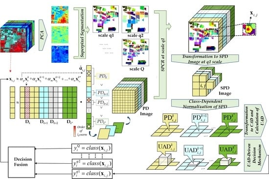
In this paper, a superpixel-level constraint representation (SPCR) model is proposed, combining a spatial constraint, simple linear iterative clustering (SLIC) superpixel segmentation, to the CR model [30]. Differing from the ACR model, the proposed SPCR method extracts the spectral–spatial information of pixels inside the superpixel block, preserves most of the edge information in the image, and estimates the real distribution of ground objects [31]. In general, the SPCR model utilizes the spectral feature of adjacent pixels, and transforms the individual PD to united activity degree (UAD) through a relaxed and adaptive constraint. As shown on the right side of Figure 1, the decision mechanism of the SPCR model is to classify the testing pixel into the category with the maximum UAD. However, like most OBIC-based methods, the constrained representation classification with a single fixed scale needs to find the optimal scale. To address this issue, it is necessary to propose a multiscale OBIC framework to comprehensively utilize image information [32]. As illustrated in Figure 1, we proposed an improved version based on the above SPCR model, called the multiscale superpixel-level constraint representation (MSPCR) method.
The MSPCR merges the classification maps generated by SPCR at different superpixel segmentation scales, which is implemented in three steps: (1) a segmentation step, in which the processed hyperspectral image is segmented into superpixel images with different scales by the SLIC algorithm; (2) a classification step, in which the PD of pixels inside the superpixel is utilized to shape the class-dependent constraint of the testing pixel; and (3) a decision fusion step, in which the final classification map of MSPCR is obtained through the decision fusion processed, based on the classification result of SPCR at each scale.
As mentioned above, the CR model classifies the testing pixel based on the PD-driven decision mechanism, and obtains a reliable performance with relatively low computational time. Considering the influence of the spectral variability, the ACR model adopts the PD of adjacent pixels to obtain the category of the testing pixel. However, the ACR only regards the pixels within a fixed window as adjacent pixels, lacking consideration to the correlation of ground objects. To address this issue, the SPCR model is firstly established by joining the CR model with the SLIC superpixel segmentation algorithm. Then, the MSPCR approach is successively proposed to alleviate the impact of the segmentation scale on the classification result of the SPCR method, and obtains high accuracies. Experimental results on four real hyperspectral datasets including a GF-5 satellite data are used to evaluate the classification performance of the proposed SPCR and MSPCR methods.
The rest of this paper is organized as follows. Section 2 reviews the related models, including classic representation-based classification methods and superpixel segmentation algorithm, i.e., SLIC that we used in this paper. Section 3 presents our proposed methods, firstly introduces the CR method and the ACR classifier, then presents the SPCR model and the MSPCR method proposed in this paper. Section 4 evaluates the classification performance of our proposed methods and other related methods via the experimental results on three real hyperspectral datasets. Section 5 takes a practical application and analysis to our proposed methods via the experiment on a GF-5 satellite data. Section 6 concludes this paper with some remarks.
2. Related Methods
In this section, we introduce several related methods of our framework. The classic sparse representation (SR)-based model and the joint representation (JR)-based framework are firstly reviewed in Section 2.1. Then the simple linear iterative clustering (SLIC) is presented in Section 2.2.
2.1. Representation-Based Classification Methods
Defining a testing pixel in the location of HSI which contains spectral bands and pixels ( and index the row and column of scene). The dictionary can be denoted as , in which each column of is the samples selected from class ( is the number of classes).
2.1.1. Sparse Representation-Based Model
Since pixels in HSI can be represented sparsely, representation-based methods have been widely applied to process HSI due to their no assumption of data density distribution [33]. The SRC is a classic SR-based model, implementing classification based on several steps as follows. Firstly, it constructs a dictionary by training the available labeled samples, then represents the testing pixel by a sparse linear combination of the dictionary. Moreover, in order to use as few labeled samples as possible to represent the testing pixel, the weighted coefficients used in representation are sparsely constrained. Finally, the classification is conducted by a residual error-driven decision mechanism, which classifies the testing pixel as the class with minimum class-dependent residual error using the following formula:
where denotes the l1-norm and is the l2-norm, due to the optimization of l0-norm is a combinatorial NP-hard problem, the sparse constraint of weight coefficients adopts l1-norm to substitute l0-norm, where l1-norm is the closet convex function to the l0-norm. Moreover, is a scalar regularization parameter. As an indicator function, can assign zero to the element that does not belong to the class . The weight vector, , can be optimized by the basis pursuit (BP) or basis pursuit denoising (BPDN) algorithm.
2.1.2. Joint Representation-Based Framework
HSIC initially focused on the spectral information because of its data characteristic, while the spatial information can be further exploited to reduce classification errors, according to the similar spectral characteristic among neighborhood pixels. As the second generation of SRC, the joint SRC (JSRC) is introduced under the JR-based framework, which has a solid classification performance after integrating spectral information with the local spatial coherence.
Based on the local spatial consistency, the fundamental assumption of JSRC is that the sparse vectors related with the adjacent pixels could share a common sparsity support [34]. In the JSRC, both the testing pixel and its neighboring pixels are stacked into the joint signal matrix, and sparsely represented using the dictionary and a row-sparse coefficient matrix [35]. The final classification result of JSRC is obtained by calculating the minimum total residual error as follows:
where is a pixel-sized square neighborhood centered on , and is the corresponding coefficient matrix. is the Frobenius norm and is the l1,2-norm, in which is the s-th row of .
2.2. Simple Linear Iterative Clustering
The OBIC is a widely used spectral–spatial classification framework, and it utilizes the spatial information after the procedure of segmentation [36]. As one of the widely used segmentation methods, the SLIC algorithm identifies superpixels by the over-segmentation approach. The idea of SLIC is to locally apply the K-means algorithm to obtain an effectively cluster segmentation result. Specifically, it measures the distance from each cluster center to pixels within a block, where . Here, is the number of pixels, and is the number of clustering centers which equals to the total number of superpixels [37].
In general, the SLIC algorithm can be implemented in several steps as follows: the first step is to select initial clustering centers from the original image. Then it classifies each pixel to the nearest clustering center, and constructs various clusters respectively. The iterative clustering process is performed until the position of the cluster center became stable. As stated above, the original K-means algorithm calculates the distance from the whole map, while the searching area of SLIC is in the local area of each superpixel, thereby the SLIC algorithm alleviates the computation complexity to a great extent. The distance in SLIC is defined as follows:
where is a spectral distance, which is used to ensure the homogeneity inside the superpixel, and the spectral distance between pixel and pixel is described as follows:
where is the value of pixel in band , and represents the spatial distance, which is used to control the compact and regularity of the superpixels, the spatial distance between pixel and pixel is defined as follows:
where is the location of pixel , , and in Equation (3) are the scale parameter of superpixels.
3. Proposed Approach
As introduced in Section 2.1, both the classic SR-based model and the variant JR-based method conduct the classification using the class-dependent minimum residual error between the original observation and the approximate representation value. However, the residual error-based decision mechanism in the SR-based and JR-based frameworks ignore the importance of sparse coefficients. Section 3.1 introduces that the CR method and the ACR classifier can exploit the characteristic of the sparse coefficient. After that, we present the details of SPCR and the MSPCR in Section 3.2. Both methods are generally based on the spatial correlation. Specifically, the SPCR utilizes the spectral consistency feature among adjacent pixels in ACR, and then MSPCR achieves comprehensive utilization of various regional distribution.
3.1. Constraint Representation (CR) and Adjacent CR (ACR)
3.1.1. CR Model
According to the principle of representation-based model, it can be regarded as representing the testing pixel via a sparse linear combination of the labeled samples. For the sake of understanding, a simple case can be assumed as Equation (6). The testing pixel is represented by a single element with nonzero coefficient () from some certain classes () as follows [38]:
Since is sparsely constrained, the labeled samples which contributes to representing the testing pixel are the ones whose coefficients are not zero. In the process of representation, the larger measurement of the coefficient value, the higher contribution in representing the testing pixel, such that the testing pixel more likely belongs to the corresponding category. Therefore, CR directly exploits the sparse coefficient to conduct the classification, which is concise and equivalent to the residual error-driven determination mechanism. Specifically, it defines the participant degree (PD) from the perspective of the sparse coefficient, which estimates the contribution of labeled samples from different classes in representing the testing pixel . The PD of each class is calculated by the corresponding weight vector with ld-normed measurement (d = 1 or d = 2) as follows:
The PD-driven decision mechanism of CR is to determine the category with the maximum PD, which can be expressed in Equation (8):
3.1.2. ACR Model
Based on the PD-driven mechanism, an improved version, ACR has been proposed to correct spectral variation by imposing spatial constraints during the classification. According to the spectral similarity characteristic among the adjacent pixels, the adjacent pixels more likely belong to the same class [39]. In this context, the ACR brings better classification performance than that of the CR model through innovating the PD-driven mechanism with the spatial consistency of the adjacent pixels. The main principle of ACR is to use the PD of adjacent pixels as a constraint to determine the category of the testing pixel. Specifically, the ACR firstly defines adjacent pixels within a pixel-sized window centered on the testing pixel, then constructs a k-dimensional PD image, and each dimensionality of the PD image shows the PD values of pixels in one class. The class-dependent activity degree (CAD) of each element is obtained after successively normalizing the PD image at each dimensionality, which could be expressed as follows:
where denotes the class index, and are the location of the testing pixel. With consideration of the spatial constraint of the adjacent pixels, the relative activity degree (RAD) is generated by combining the CAD of the testing pixel with the inactivity degree of its adjacent pixels through a scale compensation parameter , where the index of the adjacent pixels is . The ACR uses the RAD as the final contribution degree in representing the testing pixel , and the class of can be determined by the maximum RAD as follows:
3.2. Superpixel-Level CR (SPCR) and Multiscale SPCR (MSPCR)
3.2.1. SPCR Model
As mentioned above, the ACR model defines the adjacent pixels as pixels within a fixed pixel-sized window centered on the testing pixel. However, it does not consider the real distribution of ground objects. The superpixel block obtained by the superpixel segmentation algorithm is made up of some neighborhood pixels with similar spatial characteristics. Through combing the superpixel segmentation algorithm, we establish the SPCR model to further utilize the spectral consistency feature from the subset of adjacent pixels. In this way, the SPCR model conducts class-dependent constrained represent according to the PD of pixels inside the superpixel block centered on the testing pixel, which preserves most edge information of image in comparison to the sample selection in fixed window in ACR, and has a more objective consideration to the spatial distribution of the testing pixel. As illustrated in Figure 1, the schematic diagram of SPCR model is equal to MSPCR at a single segment scale, which can be implemented in several steps as follows.
Firstly, we obtain superpixel blocks by the SLIC algorithm. Since the SLIC can only process an image in the CIELAB color space, it is necessary to convert an HSI to a three bands image before processed by the SLIC algorithm. Therefore, the principal component analysis (PCA) method is adopted to reduce the spectral dimensionality in the SPCR method, which selects the first three components as the input of SLIC to generate a stable superpixel segmentation result [40]. Then, the category of the testing pixel can be measured by calculating the PD values of pixels inside the superpixel where the testing pixel is located. Specifically, using the PD values of pixels at the corresponding position of the superpixel, we built a SPD image surrounding with dimension, and each dimension of SPD image shows the PD values of pixels in one class. Similar to ACR, the normalized value of each pixel in the SPD image is defined as the class-dependent activity degree (CAD) with regard to the class .
In order to further utilize the correlation of ground objects, SPCR combines the CAD of with CAD of other pixels insides superpixel through the scale compensation parameter, such that other pixels can give a properly constraint in classifying the testing pixel . Compared to the constraint with the local spatial information in RAD shown in formula (10), the united activity degree (UAD) utilizes the correlation of ground object via a similar combination, represented as follows:
where indicates the element index in superpixel block, represents a scale compensation parameter. Moreover, the SPCR model classifies by analyzing which class leads to the maximum as follows:
3.2.2. MSPCR Model
As shown in the aforementioned algorithm, the proposed SPCR method based on the OBIC framework generates solid performance through exploiting the spatial contextual information. However, as the classification results of SPCR with different segmentation scales are not the same, the superpixel segmentation-based HSI classification may not generate a comprehensive and stable result under a fixed segmentation scale. Thus, in particular, the performance of SPCR is highly affected by the scale level [41]. In order to solve these problems, it is reasonable to propose multiscale OBIC framework to comprehensively utilize image information. In this paper, MSPCR is firstly proposed by means of decision fusion with the classification result maps obtained by SPCR method at different segmentation scales. Compared with SPCR, the improved MSPCR not only uses multiple scales to balance the different size and distribution of ground objects, but also solves the problem of selecting the optimal segmentation scale.
Specifically, Figure 1 and Algorithm 1 illustrate the general schematic diagram and pseudo procedures of the MSPCR method, respectively. Firstly, similar to the workflow of the SPCR method, we simultaneously obtain the classification results of the testing pixel at different superpixel segmentation scales. In this process, the superpixel block is generated by inputting the result of PCA into the SLIC algorithm, then classify the testing pixel by a relaxed and adaptive constraint inside the superpixel. After performing the SPCR method at each scale, a decision fusion process is applied to obtain the classification result of MSPCR, in which the category of the testing pixel is determined by the maximum number of labels of the testing pixel among the classification results at each scale, and the decision fusion process is expressed as follows:
where is denoted as the final class label of , represents the classification result of when the segmentation scale parameter is described as , and mod is a modular function which defines with the most frequency category in .
| Algorithm 1. The proposed MSPCR method |
| Input: A hyperspectral image (HSI) image , dictionary , the testing pixel , regularization parameter , scale compensation parameter . |
| Step 1: Reshape into a color image by compositing the first three principal component analysis (PCA) bands. Step 2: Obtain multiscale superpixel segmentation images of according to SLIC in Equations (3) to (5). Step 3: Obtain the participation degree (PD) image of according to Equation (7). Step 4: Extract superpixel centered on the testing pixel from the PD image of to get multiscale SPD image. Step 5: Class-dependent normalization at each scale according to Equation (9). Step 6: Calculate the united activity degree (UAD) according to Equation (11). Step 7: Assign the class of at each scale according to Equation (12). Step 8: Determine the final class label by the decision fusion according to Equation (13). Output: The class labels . |
4. Experimental Results and Analysis
In this section, we investigated the effectiveness of the proposed SPCR and MSPCR models with three hyperspectral datasets. The detailed description of the applied datasets is given in Section 4.1. The parameter tuning related to the proposed models and other compared methods is presented in Section 4.2. We evaluate the performance of two proposed methods in comparison with the methods in the spectral domain and the spectral–spatial domain. The classic SR-based method, including SRC as well as its simplified model CR, and the classic SVM are firstly selected in the comparative experiments in the spectral domain. Then, the classic JR-based model JSRC, the typical model with post-processing of spatial information SVM-MRF, and the previously proposed ACR are further tested in the spectral–spatial domain. We randomly selected training samples 20 times in each experiment and calculated the overall accuracy (OA) and class-dependent accuracy (CA). We analyzed the experimental results of the two proposed methods and other related methods in Section 4.3, Section 4.4, and Section 4.5.
4.1. Experimental Data Description
4.1.1. Airborne Visible/Infrared Imaging Spectrometer (AVIRIS) Indian Pines Scene
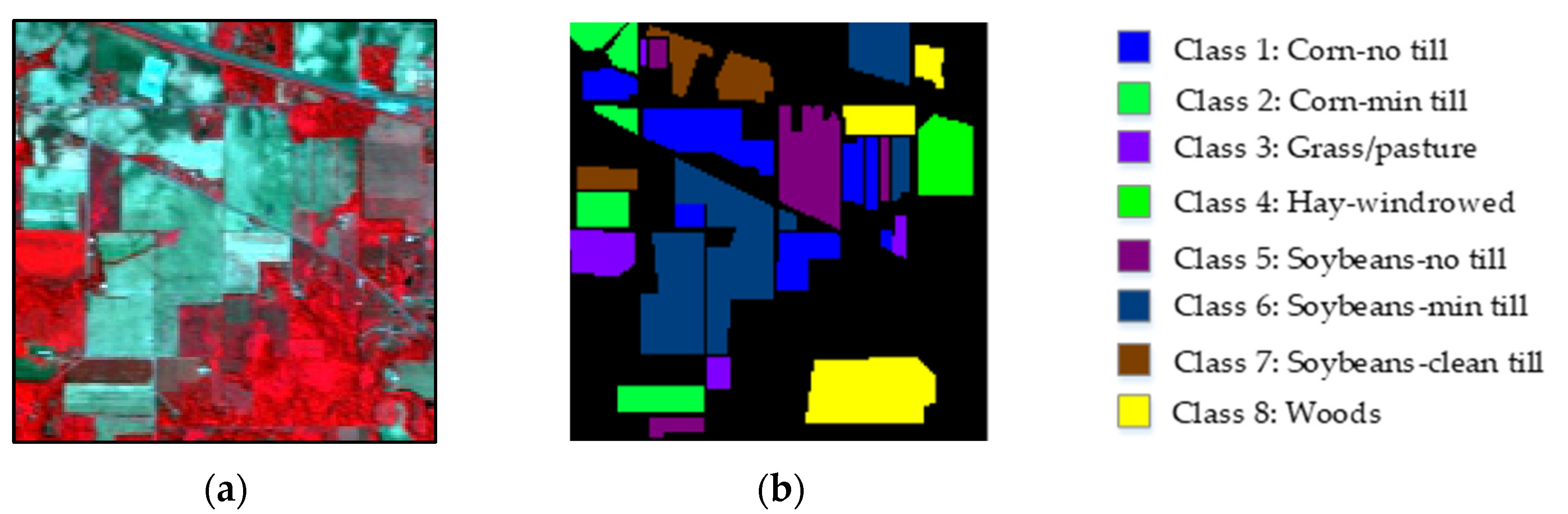
The first data are of the Indian Pines scene acquired by the Airborne Visible/Infrared Imaging Spectrometer (AVIRIS) sensors in the Northwestern Indiana, with a spatial resolution of 20 m. The scene covers 220 spectral bands ranging from 0.4 to 2.5 μm, and the size of the image is . In order to satisfy the sparse thought, eight ground-truth classes with a total of 8624 labeled samples are extracted from the original sixteen categories reference data. Figure 2a,b shows the false-color composite image and the reference map of this scene, respectively.
4.1.2. Reflective Optics Spectrographic Imaging System (ROSIS) University of Pavia Scene
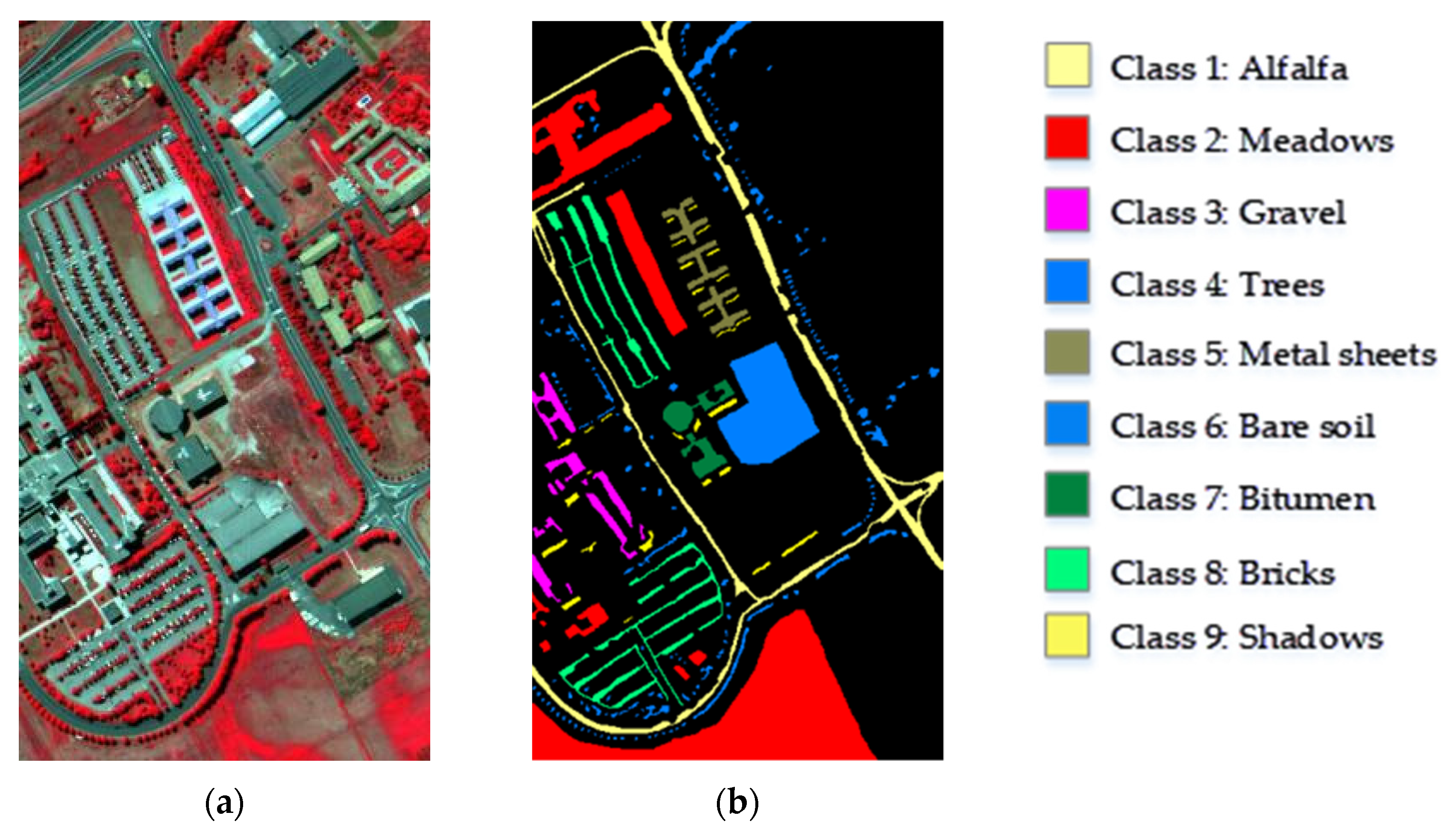
The second data are of the University of Pavia scene collected by the Reflective Optics Spectrographic Imaging System (ROSIS) over a downtown area near the University of Pavia in Italy, with a spatial resolution of 1.3 m. After removing 12 bands with high noise and water absorption, the scene has 103 spectral bands ranging from 0.43 to 0.86 μm, with pixels. Nine ground-truth classes with a total of 42,776 labeled samples are contained in the reference data. Figure 3a,b shows the false-color composite image and the reference map of this scene, respectively.
4.1.3. Hyperspectral Digital Image Collection Experiment (HYDICE) Washington, DC, National Mall Scene
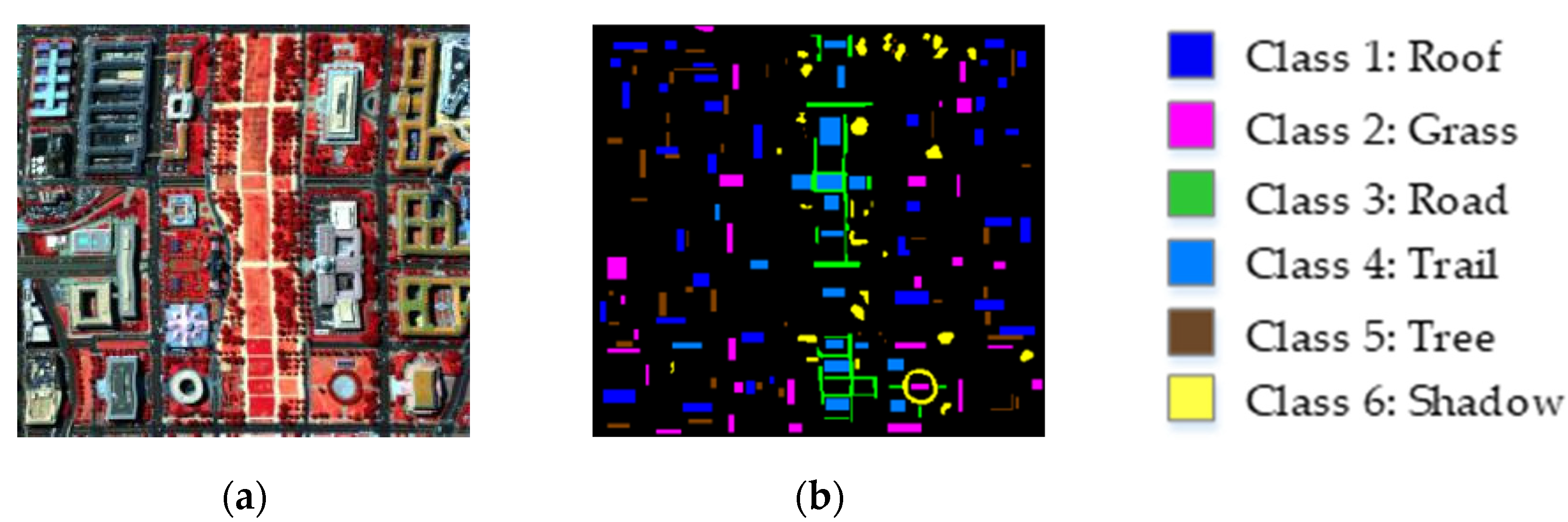
The third data are of the Washington, DC, National Mall scene captured by the Hyperspectral Digital Image Collection Experiment (HYDICE) sensor over the Washington, DC, in USA, with a spatial resolution of 3 m. The original scene contains 210 spectral bands ranging from 0.4 to 2.5 μm, with pixels. After removing the atmospheric absorption bands from 0.9 to 1.4 μm, 191 bands were remaining. Six ground-truth classes with a total of 10190 labeled samples were included in the reference data. Figure 4a,b shows the false-color composite image and the reference map of this scene, respectively.
4.2. Parameter Tuning
In the experiment of this paper, the regularization parameter for all SR-based models was selected from to . For the scale compensation parameter and in ACR and SPCR-based methods, we set them in a properly range according to the value of and the number of superpixels . Due to the different value of , the distributions of the ground objects in the pixel-sized window centered on the testing pixel are different. This fact produces a critical constraint based on the assumption that the adjacent pixels inside the window belong to the same class. Referring to the definition of in [22], each scene usually has a proper with a consideration of the spatial consistency, and the exceeded size could influence the result. Therefore, in order to obtain a high classification accuracy, we optimized the size of the window in each experimental scene.
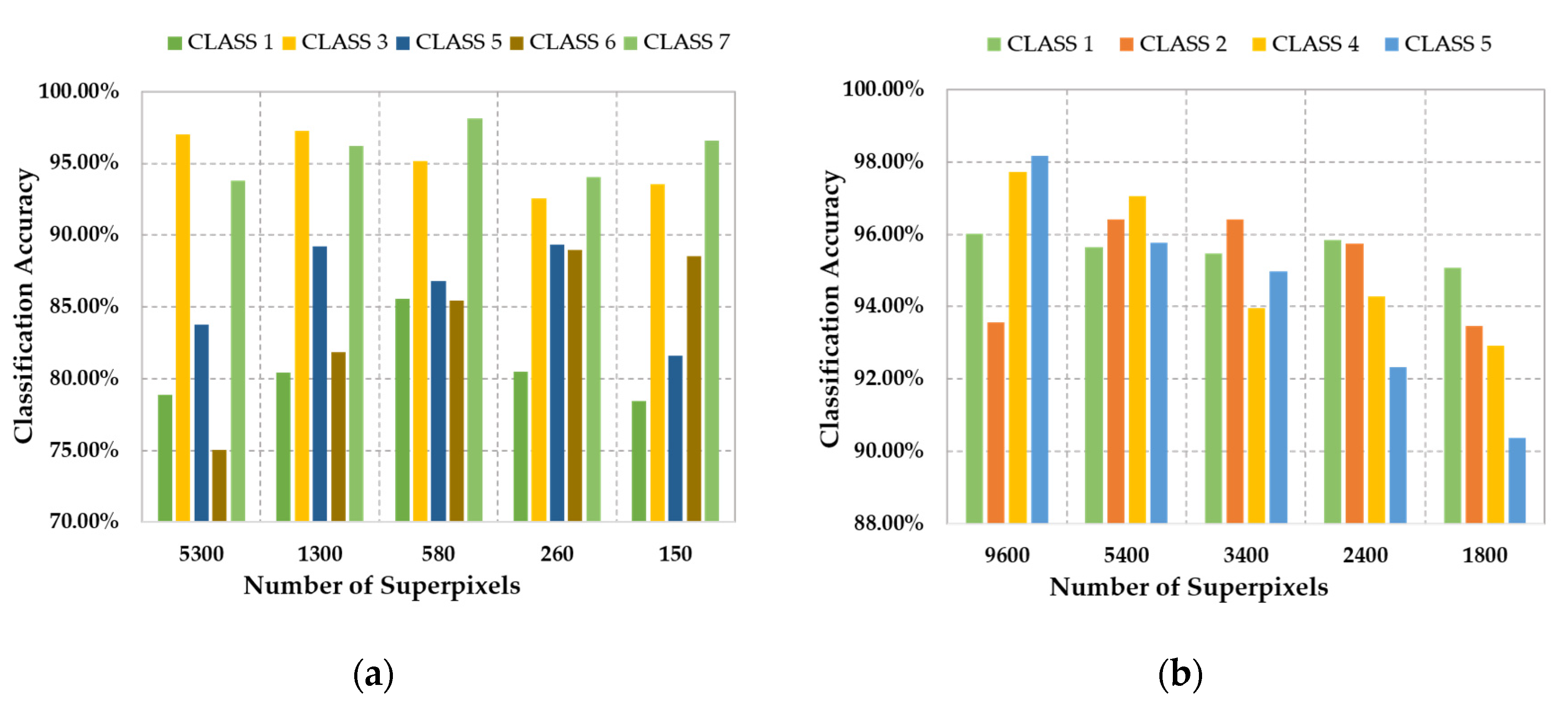
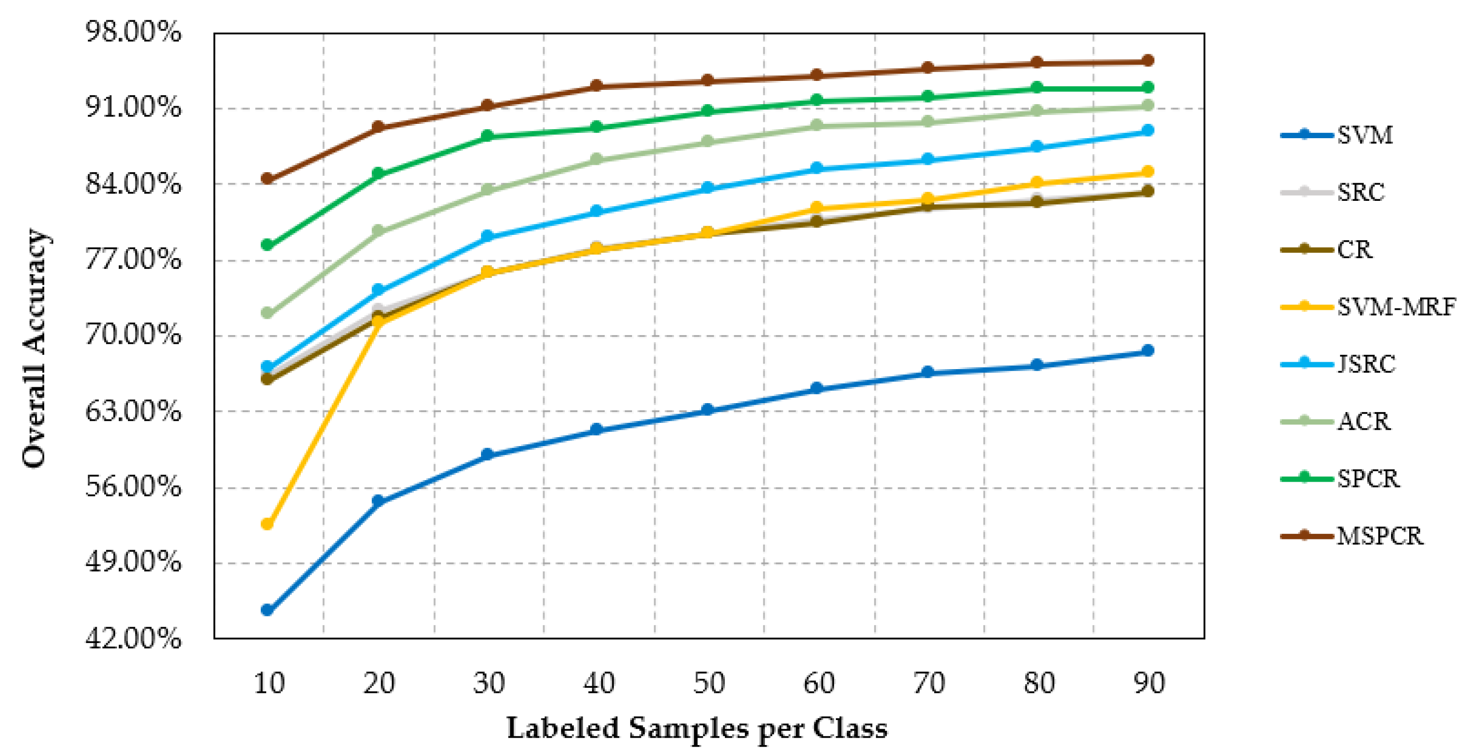
In addition, the number of superpixels in SPCR and MSPCR classifier is decided by the segmentation scale and the number of the pixels via . The corresponding experimental analysis about and the classification accuracy is illustrated in Figure 5 and Figure 6. We can infer the relationship between the segmentation scale and the classification accuracy, which is equal to the relationship of and the classification results. Firstly, Figure 5 shows the impact of the number of superpixels on the classification accuracy (50 samples per class). We mainly select five and four classes to display from the AVIRIS Indian Pines dataset and HYDICE Washington, DC, National Mall dataset, respectively. As illustrated in Figure 5a, the result indicates that the optimal segmentation scale is various for different classes. For example, the optimal segmentation scale of the class 2 is distinct from the other three classes in Figure 5b. In addition, the relationship of the number of superpixels, overall accuracy and the number of the labeled samples is shown in Figure 6. Generally, the overall accuracy increased with the number of labeled samples at each segmentation scale. It is notable that under different number of labeled samples, the segmentation scale is various in order to achieve the highest classification accuracy. Like the most OBIC frameworks, the proposed SPCR method also needs to set the optimal segmentation scale, while the improved MSPCR method can overcome this drawback through taking fusion the spatial–spectral characteristics of HSI at different segmentation scales.
4.3. Experiments with the AVIRIS Indian Pines Scene
In the first experiment with the AVIRIS Indian Pines hyperspectral scene, we randomly selected 90 labeled samples per class with a total of 720 samples to construct a dictionary and the training model. The selected training samples constitutes the approximately 8.35% of the labeled samples in the reference map, and the other remained samples are used in validation. As illustrated in Table 1, the OAs and the CAs of different methods are calculated, and the corresponding classification maps are presented in Figure 7. We analyzed the classification results as follows:
- 1
- As a widely applied supervised classification framework, the SVM classifier has a feasible performance in the classification of HSI. However, there are some isolated pixels appeared in the result due to the noise and spectral variability, as shown in Figure 7. Compared with the SVM, the classic SRC method gains a better classification result, which proves that the SR-based classifier is suitable for the hyperspectral image classification tasks. Compared with the SRC, the CR model obtains an approximate equivalent classification result with a lower computational cost than that of SRC. The result not only underlines the CR model simplified the SRC model via an improved procedure without the calculation of residual error, but also verifies the effectiveness of the PD-driven decision mechanism in the process of HSIC.
- 2
- In the spectral–spatial domain, as shown in Figure 7, SVM-MRF model outperforms the SVM classifier, which demonstrates the exploration of the spatial information can bring a further improvement on the spectral classifiers. Similarly, since the JSRC conducts the classification by sharing a common sparsity support among all neighborhood pixels, the improvement of overall accuracy also appeared in JSRC compared to SRC. Compared with the CR model, the ACR classifier obtains a significant improvement. It solves the spectral variability problem in CR by setting a spatial constraint, and proves that the innovation of decision mechanism from PD-driven to RAD-driven is effective for the HSIC tasks. As mentioned above, the improvements of SVM-MRF, JSRC, and ACR models relative to their original counterparts SVM, SRC, and CR confirm the effectiveness of introducing spatial information into the spectral domain classifiers.
- 3
- From Figure 7, the JSRC has a better classification performance than the SVM-MRF in the AVIRIS Indian Pines scene. As illustrated in Table 1, the ACR classifier achieves a better classification result in comparison to JSRC and SVM-MRF, of which the overall accuracy is 2.38% higher than that of JSRC and 6.11% higher than that of SVM-MRF. On one hand, the RAD-driven mechanism in ACR is more effective than the hybrid norm constraint in JSRC. On the other hand, the post-processing of spatial information in SVM-MRF takes more emphasis on adjusting the initial classification result generated from spectral features, lacking an effective strategy integrating spatial information with spectral information.
- 4
- Compared with the ACR, the proposed SPCR has a slightly higher OA. Table 1 demonstrates the effectiveness of introducing the superpixel segmentation, which preserves the edge information and fully considers the distribution of ground object. In addition, the practicability and reliability of the sparse coefficient, which plays an important role in the PD-driven decision mechanism and the UAD-driven decision mechanism. Thus, the combination of superpixel segmentation and sparse coefficients is effective, the overall accuracy of SPCR reaches to 92.90%, which is 1.66%, 4.04%, and 7.77% higher than ACR, JSRC, and SVM-MRF, respectively.
- 5
- Compared with the SPCR, the proposed MSPCR model brings an improvement. Firstly, it verifies that the MSPCR performs better than the SPCR via alleviating the impact of superpixel segmentation scale on the classification results. Then, it also indicates that the decision fusion takes a comprehensive consideration to the different spatial features and distributions of various categories of objects, which elevates the final classification accuracy.
In general, the proposed MSPCR obtains an overall accuracy of 95.30%, which is 2.40% and 4.06% higher than SPCR and ACR, and also 12.11% higher than CR, respectively. For individual class accuracy, it provides great results, especially for the classes 2, 6, and 7. The classification maps in Figure 7 verify the improvement achieved by the MSPCR.
In the second test with the AVIRIS Indian Pines scene, we randomly selected 10 to 90 samples per class as the training samples to measure the proposed SPCR and MSPCR. Figure 8 shows the overall classification accuracies acquired by different methods with different number of labeled samples. The results can be summarized as follows:
- The classification results demonstrate that the overall accuracy has a positive relationship with the number of the labeled samples, the overall accuracy is increased by the number of labeled samples. Besides, this phenomenon only be satisfied under a certain number of the labeled samples, the growth trend would be stopped when the labeled samples reach a certain number.
- The integration of the spatial and spectral information benefits precision classification than the pixel-based classification method, which can be verified by the improvement of SVM-MRF, JSRC, ACR, SPCR, and MSPCR relative to their original counterparts, i.e., SVM, SRC, and CR.
- Compared to the traditional classifiers, the PD-driven classifiers provide a better classification performance. This can be confirmed by the overall accuracies of ACR and SPCR toward JSRC and SVM-MRF, as well as CR toward SVM. Moreover, the proposed MSPCR achieved the best performance among these classifiers.
4.4. Experiments with the ROSIS University of Pavia Scene
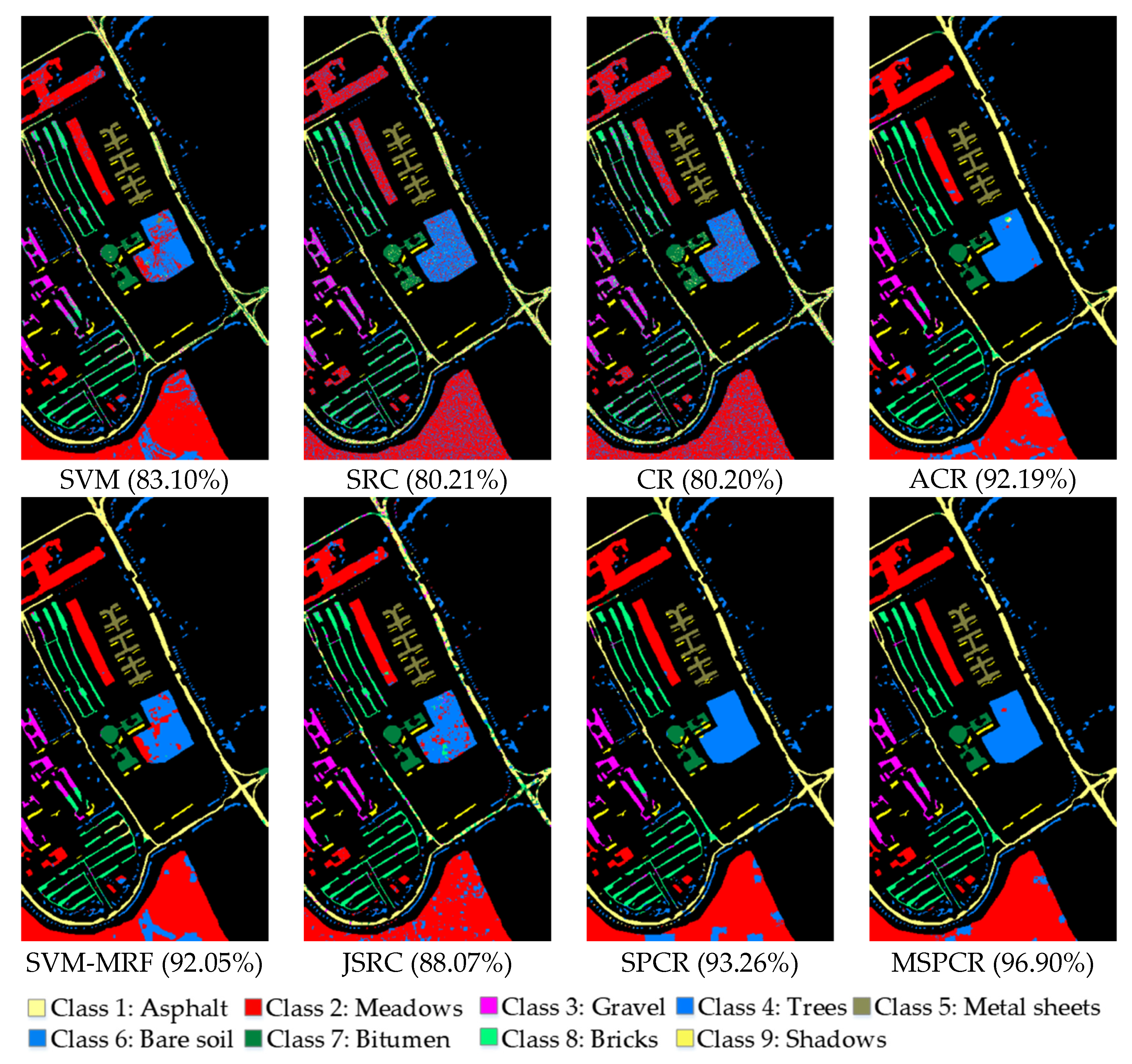
In the first test of the experiment with the ROSIS University of Pavia scene, we select 90 labeled samples per class with a total of 810 samples (which constitutes approximately 1.89% of the available labeled samples in the reference map), and the remaining labeled samples are used for validation. Table 2 and Figure 9 show the OAs and CAs for the classifiers, and the corresponding classification maps. From the experimental results, we have similar results with those obtained under the AVIRIS Indian Pines dataset: First, SRC and CR achieved similar classification results, with comparative result in comparison with the SVM in the spectral domain. In the spatial domain, SVM-MRF, JSRC, and ACR bring significant improvement to the SVM, SRC, and CR model by integrating the spatial information. Moreover, SVM-MRF owns a better classification accuracy than JSRC, different from the performance of these two methods in AVIRIS Indian Pines dataset. In comparison with the ACR, the introduction of the superpixel segmentation algorithm contributes to a higher accuracy in SPCR. Last but not the least, the proposed MSPCR achieves the best classification result with the overall accuracy of 96.90%, which is 3.64% and 4.71% higher than SPCR and ACR, and also 16.7% higher than CR, respectively. Additionally, it brings considerable improvements for individual class accuracy, especially for class 2 and class 4, which can be proved by the classification maps shown in Figure 9.
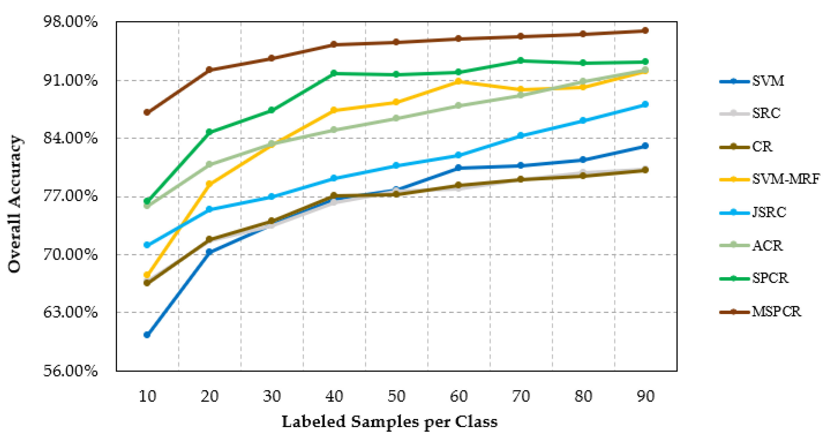
Our second test of the ROSIS University of Pavia scene measured the proposed SPCR and MSPCR with various sizes of labeled samples (from 10 to 90 samples per class). Figure 10 shows the overall classification accuracies obtained by different testing methods, under different number of training samples. With the number of the labeled sample increased, most of measured methods have an increase trend in accuracy. In comparison to the overall classification accuracy of SVM, the SRC and CR firstly have better performances, then perform worse as the number of the labeled samples increased. Considering the correlation of ground object, the classification performance of ACR and SVM-MRF, achieved significant improvements with the increase of the number of samples, with a higher classification accuracy than the JSRC in most cases. In addition, the combination of the PD-decision mechanism and the superpixel segmentation algorithm brings reliable and stable improvement, which can be confirmed by the overall classification accuracies obtained by SPCR method in all cases. From Figure 10, MSPCR method achieves the best classification result among these compared methods, as a result of applying the decision fusion which alleviates the challenge of adapting the fixed single segmentation scale to the spatial characteristic of all categories in the image.
4.5. Experiments with the HYDIC Washington, DC, National Mall Scene
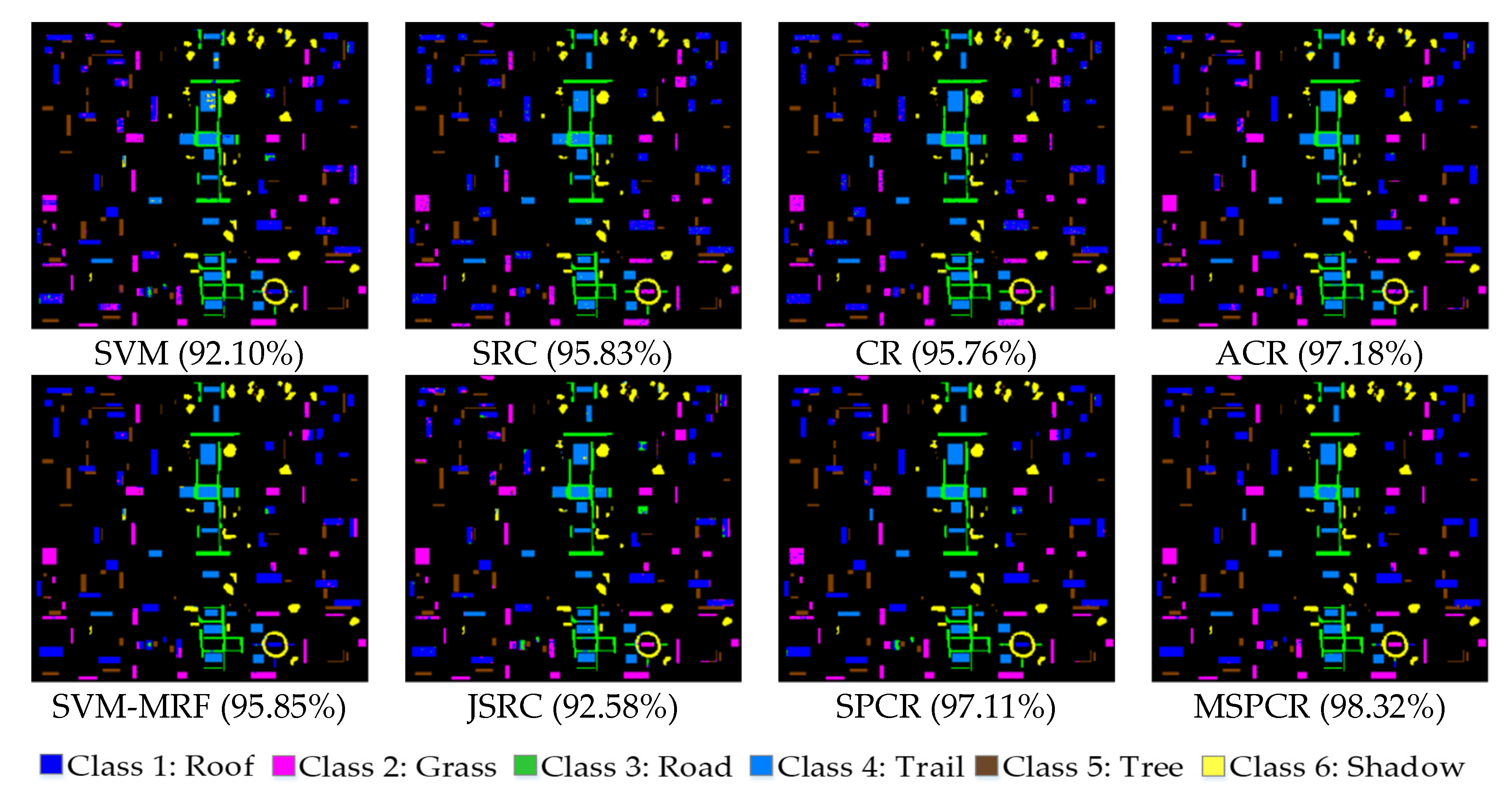
In our first test with the HYDICE Washington, DC, National Mall scene, we first randomly select 50 labeled samples per class with a total of 300 samples for training and dictionary construction (which constitutes approximately 2.94% of the available labeled samples), the remaining samples are applied for validation. Table 3 shows the OAs and CAs obtained in different tested methods, and Figure 11 shows the corresponding classification maps. In the spectral domain, the traditional SRC provides an approximately equivalent result to CR, and both of them outperform the traditional SVM method, once again proving that the sparse coefficient is powerful to represent the spectral characteristics. In the spectral–spatial domain, the SVM-MRF, ACR, and SPCR perform well toward their original counterparts, i.e., SVM and CR. In addition, it also can be seen from the overall accuracies of the SRC method and the JSRC model that an improperly spatial constraint may have a negative impact on the classification performance. Distinct from the classification results in the above two datasets, the ACR gains a better classification performance than the proposed SPCR method in the HYDICE Washington, DC, National Mall scene, indicating that the SPCR model is susceptible to the superpixel segmentation scale. That is the original intention for us to propose MSPCR method, which eliminates the impact of the number of superpixels on classification by fusing the classification results at different segmentation scales. Furthermore, it can be found that the proposed MSPCR method achieves the highest accuracy 98.32%, which is similar with the results in the AVIRIS Indian Pines hyperspectral scene and the ROSIS University of Pavia scene. In addition, the proposed MSPCR provides reliable individual classification accuracy for each class, especially for class 1 and 2, which can be seen from the classification maps in Figure 11.
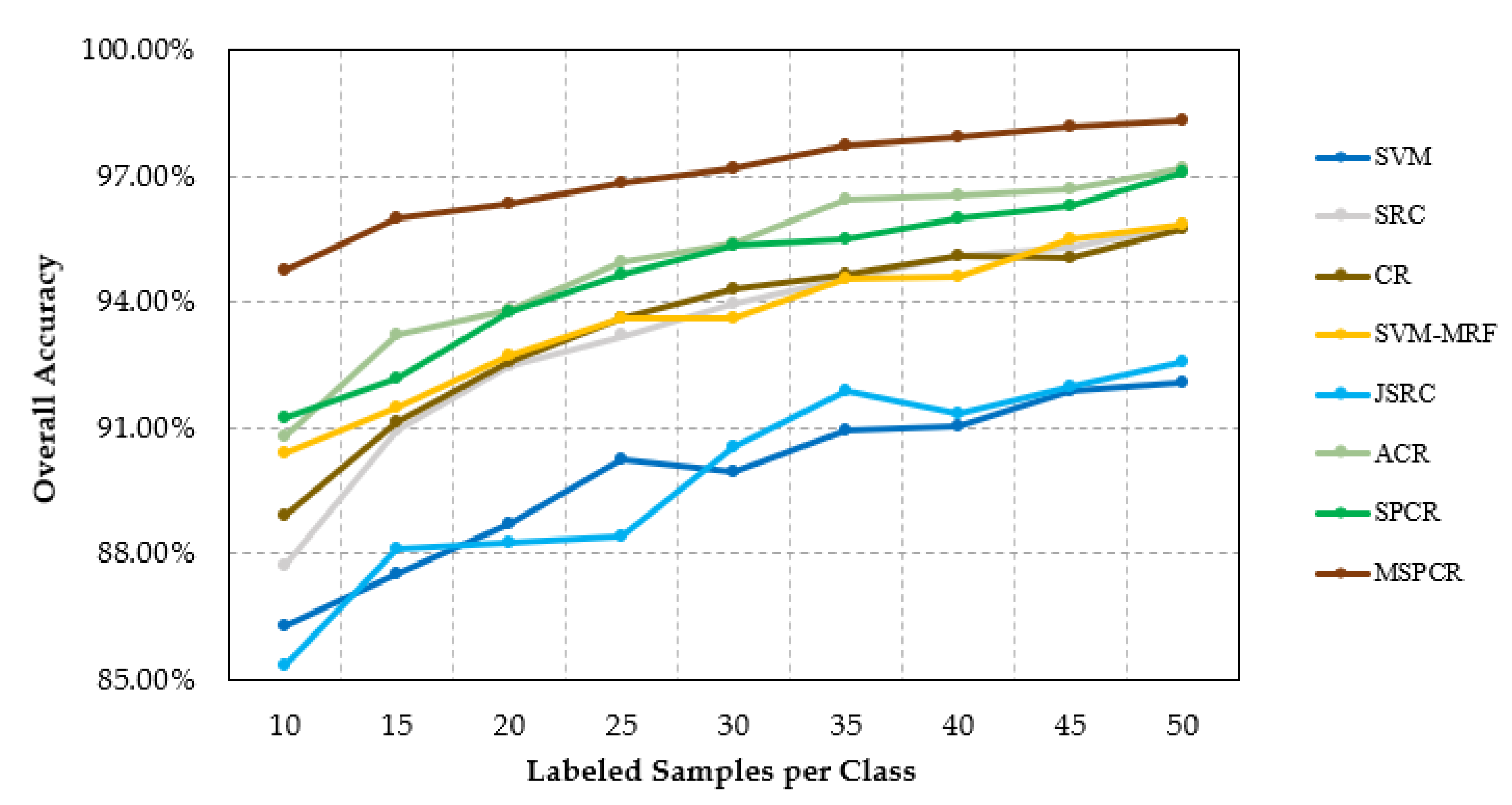
In our second test with the HYDICE Washington, DC, National Mall scene, we evaluated the classification performance of our proposed methods from the spectral–spatial domain with different numbers of training samples. As shown in Figure 12, the classification result shows a rising tendency with the increase of the number of training samples, and curve tends to be flat when the number of training samples reaches to a certain amount. Firstly, the SRC and CR gain a better classification results toward SVM with the increase of the number of the labeled samples in the spectral domain. Though JSRC obtains relatively poor results than SRC, the SVM-MRF, ACR, and SPCR still provide competitive classification performances toward the SVM and CR with the increase of the number of training samples, which proves the integration of the spectral feature discrimination and spatial coherence is a reliable processing framework for the HSIC in most cases. On the other hand, improvement also appeared by the combination of the PD-driven and spatial constraint, which is indicated by the performance of ACR and SPCR-based method versus SVM-MRF and JSRC. In the spectral–spatial domain for all cases, the proposed MSPCR yields the best overall accuracy in comparison with the other related methods, and makes a significant improvement in comparison to the proposed SPCR.
In addition, we compared the calculation cost of some spectral–spatial-based methods in the above three hyperspectral datasets, and the setting of the labeled samples corresponds to the cases in Table 1, Table 2 and Table 3. As shown in Figure 13, for the experiments on the above three datasets, the JSRC has the fastest speed but with the lowest classification accuracy. The proposed MSPCR not only achieves the best classification accuracy, which also has an increase in the time-consuming (about five times), as compared to the SPCR, due to the decision fusion process. On the ROSIS University of Pavia dataset and the AVIRIS Indian Pines dataset, the SPCR is the second best with an approximately equivalent time-consuming to ACR. On the HYDIC Washington, DC, National Mall dataset, the ACR achieves the second highest classification accuracy with a similar speed to SPCR.
Synthesizing the above experimental results and analysis, the firstly proposed SPCR method obtains a considerable overall and individual classification accuracy. The improved MSPCR gets better classification performance than the SPCR method. Moreover, the experimental results in different datasets also show that MSPCR outperforms several other related methods. Furthermore, the classification experimental results under different number of training samples also indicate the superiority and practicability of the proposed SPCR and MSPCR methods.
It should also be noted that the computational cost of the proposed MSPCR is relatively high, which is also the part of optimization in the future. Moreover, there are some potential points, for instance, the sample selection mechanism with related to the adaptive capability of method could be the follow-up research line.
5. Practical Application and Analysis
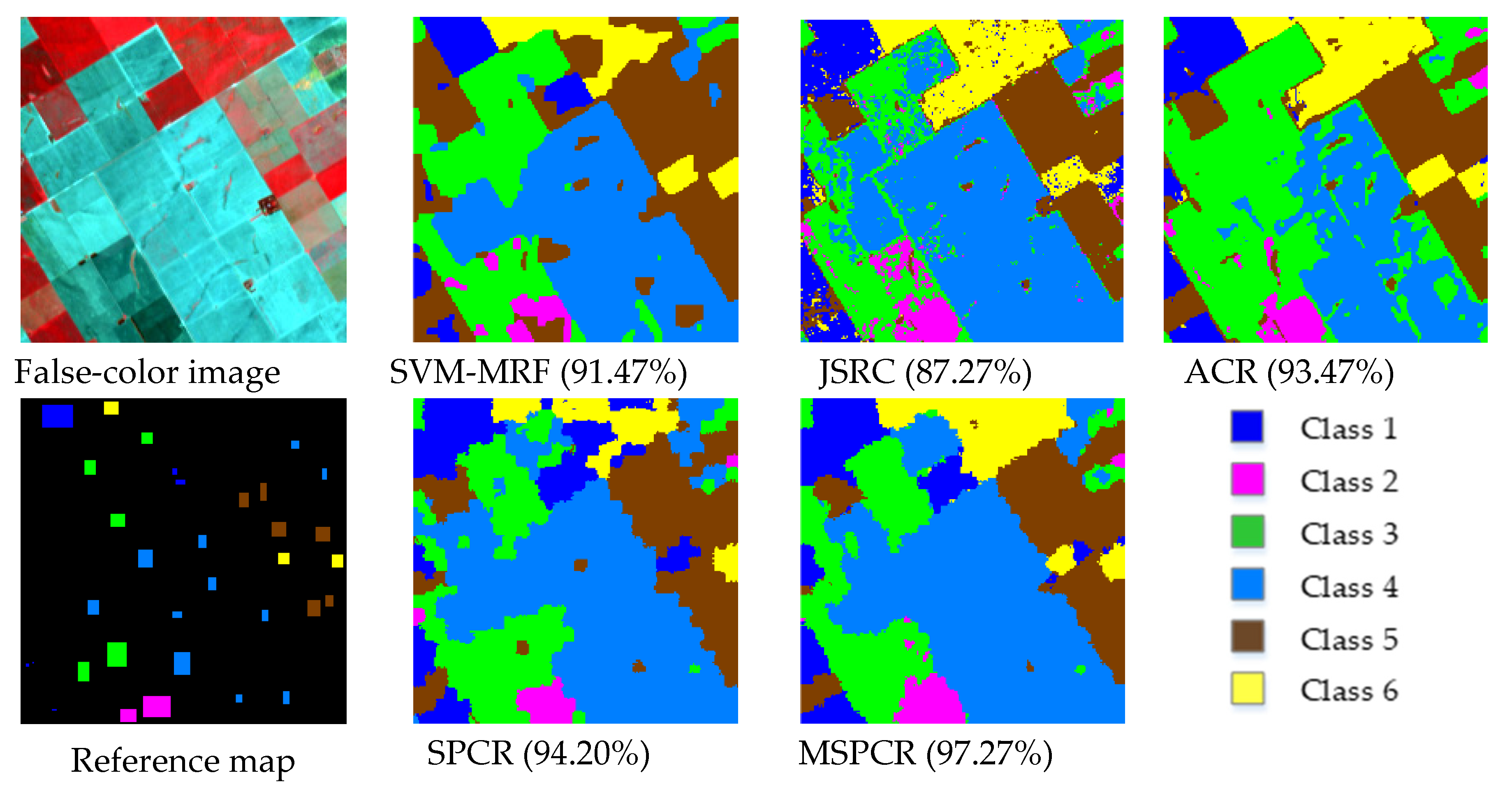
Different from the above three experimental datasets, we adopt the hyperspectral image data collected by the GF-5 satellite, to measure the practicability of the proposed SPCR and MSPCR method. GF-5 is the first hyperspectral comprehensive observation satellite of China, with a spatial resolution of 30 m. There are six payloads on GF-5, including two land imagers and four atmospheric sounders. In this paper, we select a scene from the hyperspectral image data obtained by visible short wave infrared hyperspectral camera.
First, we select the range of visible light to near infrared spectrum in the original data. After the atmospheric correction and radiation correction processing, the scene covers 150 spectral bands ranging from 0.4 to 2.5 μm, and the size of the image is . Six ground-truth classes with a total of 2216 labeled samples are contained in the reference data. Figure 14 shows the false-color composite image and the reference map of this scene.
In the experiment with the GF-5 satellite dataset, we randomly selected five labeled samples per class with a total of 30 samples to construct a dictionary and the training model. The selected training samples constitute the approximately 1.35% of the labeled samples in the reference map, and the other remaining samples are used in validation. Figure 14 displays the classification maps of different methods. We analyzed the classification results as follows:
Compared with the SVM-MRF and JSRC, the ACR has a better classification performance, of which the overall accuracy is 6.20% higher than that of JSRC and 2.00% higher than that of SVM-MRF. It confirms that the PD-driven-based decision mechanism plays an important role in classification. Compared with the ACR, the SPCR method obtains a better classification result, which verifies the effectiveness of integrating the PD-driven mechanism with the superpixel segmentation algorithm. The MSPCR outperforms the SPCR and yields the best accuracy in comparison to other related methods, which not only proves the MSPCR alleviates the impact of superpixel segmentation scale on the classification effect, but also indicates the decision fusion processing plays a decisive role in adapting different spatial characteristics of various categories of objects.
6. Conclusions
In this paper, a novel classification framework based on sparse representation, called the superpixel-level constraint representation (SPCR), was firstly proposed for hyperspectral imagery classification. SPCR uses the characteristics of spectral consistency of pixels inside the superpixel to determine the category of the testing pixel. Besides this, we proposed an improved multiscale superpixel-level constraint representation (MSPCR) method, obtaining the final classification result through fusing the classification maps of SPCR at different segmentation scales. The proposed SPCR method exploits the latent property of sparse coefficient and improves the contextual constraint, with consideration of spatial characterization. Moreover, the proposed MSPCR achieves comprehensive utilization of various regional distribution, resulting in strong classification performance. The experimental results with four real hyperspectral datasets including a GF-5 satellite data demonstrated that the SPCR outperforms several other classification methods, and the MSPCR yields a better classification accuracy than SPCR.
Author Contributions
Conceptualization, H.Y. and J.H.; formal analysis, M.S.; methodology, H.Y. and X.Z.; writing—original draft preparation, H.Y. and X.Z.; writing—review and editing, Q.G. and L.G. All authors have read and agreed to the published version of the manuscript.
Funding
This research was funded by the National Nature Science Foundation of China, grant numbers 61971082 and 61890964; Fundamental Research Funds for the Central Universities, grant numbers 3132020218 and 3132019341.
Acknowledgments
The authors would like to thank the Key Laboratory of Digital Earth Science, Aerospace Information Research Institute, Chinese Academy of Sciences for generously providing the GF-5 satellite data.
Conflicts of Interest
The authors declare no conflict of interest.
References
- Hong, D.; Gao, L.; Yokoya, N.; Yao, J.; Chanussot, J.; Du, Q.; Zhang, B. More Diverse Means Better: Multimodal Deep Learning Meets Remote-Sensing Imagery Classification. IEEE Trans. Geosci. Remote Sens. 2020. [Google Scholar] [CrossRef]
- Hong, D.; Gao, L.; Yao, J.; Zhang, B.; Plaza, A.; Chanussot, J. Graph Convolution Networks for Hyperspectral Image Classification. IEEE Trans. Geosci. Remote Sens. 2020. [Google Scholar] [CrossRef]
- He, L.; Li, J.; Liu, C.; Li, S. Recent Advances on Spectral-Spatial Hyperspectral Image Classification: An Overview and New guidelines. IEEE Trans. Geosci. Remote Sens. 2018, 56, 1579–1597. [Google Scholar] [CrossRef]
- Tong, F.; Tong, H.; Jiang, J.; Zhang, Y. Multiscale Union Regions Adaptive Sparse Representation for Hyperspectral Image Classification. Remote Sens. 2017, 9, 872. [Google Scholar] [CrossRef] [Green Version]
- Cui, B.; Cui, J.; Lu, Y.; Guo, N.; Gong, M. A Sparse Representation-Based Sample Pseudo-Labeling Method for Hyperspectral Image Classification. Remote Sens. 2020, 12, 664. [Google Scholar] [CrossRef] [Green Version]
- Gao, L.; Yao, D.; Li, Q.; Zhuang, L.; Zhang, B.; Bioucas-Dias, J.M. A New Low-Rank Representation Based Hyperspectral Image Denoising Method for Mineral Mapping. Remote Sens. 2017, 9, 1145. [Google Scholar] [CrossRef] [Green Version]
- Ghamisi, P.; Maggiori, E.; Li, S.; Souza, R.; Tarablaka, Y.; Moser, G.; De Giorgi, A.; Fang, L.; Chen, Y.; Chi, M.; et al. New Frontiers in Spectral-Spatial Hyperspectral Image Classification: The Latest Advances Based on Mathematical Morphology, Markov Random Fields, Segmentation, Sparse Representation, and Deep Learning. IEEE Geosci. Remote Sens. Mag. 2018, 6, 10–43. [Google Scholar] [CrossRef]
- Rasti, B.; Hong, D.; Hang, R.; Ghamisi, P.; Kang, X.; Chanussot, J.; Benediktsson, J.A. Feature Extraction for Hyperspectral Imagery: The Evolution from Shallow to Deep (Overall and Toolbox). IEEE Geosci. Remote Sens. Mag. 2020. [Google Scholar] [CrossRef]
- Gao, L.; Li, J.; Khodadadzadeh, M.; Plaza, A.; Zhang, B.; He, Z.; Yan, H. Subspace-Based Support Vector Machines for Hyperspectral Image Classification. IEEE Geosci. Remote Sens. Lett. 2015, 12, 349–353. [Google Scholar]
- Wang, K.; Cheng, L.; Yong, B. Spectral-Similarity-Based Kernel of SVM for Hyperspectral Image Classification. Remote Sens. 2020, 12, 2154. [Google Scholar] [CrossRef]
- Paoletti, M.E.; Haut, J.M.; Tao, X.; Miguel, J.P.; Plaza, A. A New GPU Implementation of Support Vector Machines for Fast Hyperspectral Image Classification. Remote Sens. 2020, 12, 1257. [Google Scholar] [CrossRef] [Green Version]
- Hu, S.; Peng, J.; Fu, Y.; Li, L. Kernel Joint Sparse Representation Based on Self-Paced Learning for Hyperspectral Image Classification. Remote Sens. 2019, 11, 1114. [Google Scholar] [CrossRef] [Green Version]
- Yu, H.; Gao, L.; Li, J.; Li, S.S.; Zhang, B.; Benediktsson, J.A. Spectral-Spatial Hyperspectral Image Classification Using Subspace-Based Support Vector Machines and Adaptive Markov Random Fields. Remote Sens. 2016, 8, 355. [Google Scholar] [CrossRef] [Green Version]
- Jia, S.; Deng, B.; Zhu, J.; Jia, X.; Li, Q. Superpixel-Based Multitask Learning Framework for Hyperspectral Image Classification. IEEE Trans. Geosci. Remote Sens. 2017, 55, 2575–2588. [Google Scholar] [CrossRef]
- Gao, L.; Hong, D.; Yao, J.; Zhang, B.; Gamba, P.; Chanussot, J. Spectral Superresolution of Multispectral Imagery with Joint Sparse and Low-Rank Learning. IEEE Trans. Geosci. Remote Sens. 2020. [Google Scholar] [CrossRef]
- Yang, J.; Li, Y.; Chan, J.C.-W.; Shen, Q. Image Fusion for Spatial Enhancement of Hyperspectral Image via Pixel Group Based Non-Local Sparse Representation. Remote Sens. 2017, 9, 53. [Google Scholar] [CrossRef] [Green Version]
- Gao, Q.; Lim, S.; Jia, X. Improved Joint Sparse Models for Hyperspectral Image Classification Based on a Novel Neighbour Selection Strategy. Remote Sens. 2018, 10, 905. [Google Scholar] [CrossRef] [Green Version]
- Zhang, S.; Li, S.; Fu, W.; Fang, L. Multiscale Superpixel-Based Sparse Representation for Hyperspectral Image Classification. Remote Sens. 2017, 9, 139. [Google Scholar] [CrossRef] [Green Version]
- Li, W.; Du, Q. Collaborative Representation for Hyperspectral Anomaly Detection. IEEE Trans. Geosci. Remote Sens. 2015, 53, 1463–1474. [Google Scholar] [CrossRef]
- Wang, J.; Jiao, L.; Wang, S.; Hou, B.; Liu, F. Adaptive Nonlocal Spatial–Spectral Kernel for Hyperspectral Imagery Classification. IEEE J. Sel. Top. Appl. Earth Obs. Remote Sens. 2016, 9, 4086–4101. [Google Scholar] [CrossRef]
- Geng, J.; Wang, H.; Fan, J.; Ma, X.; Wang, B. Wishart Distance-Based Joint Collaborative Representation for Polarimetric SAR Image Classification. IET Radar Sonar Navig. 2017, 11, 1620–1628. [Google Scholar] [CrossRef]
- Yu, H.; Shang, X.; Zhang, X.; Gao, L.; Song, M.; Hu, J. Hyperspectral Image Classification Based on Adjacent Constraint Representation. IEEE Geosci. Remote Sens. Lett. 2020. [Google Scholar] [CrossRef]
- Liang, J.; Zhou, J.; Qian, Y.; Wen, L.; Bai, X.; Gao, Y. On the Sampling Strategy for Evaluation of Spectral-Spatial Methods in Hyperspectral Image Classification. IEEE Trans. Geosci. Remote Sens. 2017, 55, 862–880. [Google Scholar] [CrossRef] [Green Version]
- Yu, H.; Gao, L.; Liao, W.; Zhang, B.; Pižurica, A.; Philips, W. Multiscale Superpixel-Level Subspace-Based Support Vector Machines for Hyperspectral Image Classification. IEEE Geosci. Remote Sens. Lett. 2017, 14, 2142–2146. [Google Scholar] [CrossRef]
- Wang, J.; Zhu, C.; Zhou, Y.; Zhu, X.; Wang, Y.; Zhang, W. From Partition-Based Clustering to Density-Based Clustering: Fast Find Clusters with Diverse Shapes and Densities in Spatial Databases. IEEE Access. 2018, 6, 1718–1729. [Google Scholar] [CrossRef]
- Garg, I.; Kaur, B. Color Based Segmentation Using K-Mean Clustering and Watershed Segmentation. In Proceedings of the 2016 3rd International Conference on Computing for Sustainable Global Development (INDIACom), New Delhi, India, 16–18 March 2016; pp. 3165–3169. [Google Scholar]
- Sun, H.; Ren, J.; Zhao, H.; Yan, Y.; Zabalza, J.; Marshall, S. Superpixel based Feature Specific Sparse Representation for Spectral-Spatial Classification of Hyperspectral Images. Remote Sens. 2019, 11, 536. [Google Scholar] [CrossRef] [Green Version]
- Sharma, J.; Rai, J.K.; Tewari, R.P. A Combined Watershed Segmentation Approach Using K-Means Clustering for Mammograms. In Proceedings of the 2015 2nd International Conference on Signal Processing and Integrated Networks (SPIN), Noida, India, 19–20 February 2015; pp. 109–113. [Google Scholar]
- Jia, S.; Deng, B.; Jia, X. Superpixel-Level Sparse Representation-Based Classification for Hyperspectral Imagery. IGARSS 2016, 3302–3305. [Google Scholar] [CrossRef]
- Csillik, O. Fast Segmentation and Classification of Very High Resolution Remote Sensing Data Using SLIC Superpixels. Remote Sens. 2017, 9, 243. [Google Scholar] [CrossRef] [Green Version]
- Jia, S.; Deng, B.; Zhu, J.; Jia, X.; Li, Q. Local Binary Pattern-Based Hyperspectral Image Classification with Superpixel Guidance. IEEE Geosci. Remote Sens. 2018, 56, 749–759. [Google Scholar] [CrossRef]
- Li, G.; Li, L.; Zhu, H.; Liu, X.; Jiao, L. Adaptive Multiscale Deep Fusion Residual Network for Remote Sensing Image Classification. IEEE Trans. Geosci. Remote Sens. 2019, 57, 8506–8521. [Google Scholar] [CrossRef]
- Shao, Z.; Wang, L.; Wang, Z.; Deng, J. Remote Sensing Image Super-Resolution Using Sparse Representation and Coupled Sparse Autoencoder. IEEE J. Sel. Top. Appl. Earth Obs. Remote Sens. 2019, 12, 2663–2674. [Google Scholar] [CrossRef]
- Li, W.; Du, Q.; Xiong, M. Kernel Collaborative Representation with Tikhonov Regularization for Hyperspectral Image Classification. IEEE Geosci. Remote Sens. Lett. 2015, 12, 48–52. [Google Scholar]
- Zhang, H.; Li, J.; Huang, Y.; Zhang, L. A Nonlocal Weighted Joint Sparse Representation Classification Method for Hyperspectral Imagery. IEEE J. Sel. Top. Appl. Earth Obs. Remote Sens. 2014, 7, 2056–2065. [Google Scholar] [CrossRef]
- Zou, B.; Xu, X.; Zhang, L. Object-Based Classification of PolSAR Images Based on Spatial and Semantic Features. IEEE J. Sel. Top. Appl. Earth Obs. Remote Sens. 2020, 13, 609–619. [Google Scholar] [CrossRef]
- Xie, F.; Lei, C.; Yang, J.; Jin, C. An Effective Classification Scheme for Hyperspectral Image Based on Superpixel and Discontinuity Preserving Relaxation. Remote Sens. 2019, 11, 1149. [Google Scholar] [CrossRef] [Green Version]
- Zhu, L.; Wen, G. Hyperspectral Anomaly Detection via Background Estimation and Adaptive Weighted Sparse Representation. Remote Sens. 2018, 10, 272. [Google Scholar]
- Yu, H.; Gao, L.; Liao, W.; Zhang, B.; Zhuang, L.; Song, M.; Chanussot, J. Global Spatial and Local Spectral Similarity-Based Manifold Learning Group Sparse Representation for Hyperspectral Imagery Classification. IEEE Trans. Geosci. Remote Sens. 2020, 58, 3043–3056. [Google Scholar] [CrossRef]
- Li, S.; Ni, L.; Jia, X.; Gao, L.; Zhang, B.; Peng, M. Multi-Scale Superpixel Spectral–Spatial Classification of Hyperspectral Images. Int. J. Remote Sens. 2016, 37, 4905–4922. [Google Scholar] [CrossRef]
- Jia, S.; Deng, X.; Zhu, J.; Xu, M.; Zhou, J.; Jia, X. Collaborative Representation-Based Multiscale Superpixel Fusion for Hyperspectral Image Classification. IEEE Trans. Geosci. Remote Sens. 2019, 57, 7770–7784. [Google Scholar] [CrossRef]
Figure 1.
The workflow of multiscale superpixel-level constraint representation (MSPCR).

Figure 2.
The Airborne Visible/Infrared Imaging Spectrometer (AVIRIS) Indian Pines scene: (a) false-color composite image and (b) reference map.
Figure 2.
The Airborne Visible/Infrared Imaging Spectrometer (AVIRIS) Indian Pines scene: (a) false-color composite image and (b) reference map.

Figure 3.
The Reflective Optics Spectrographic Imaging System (ROSIS) University of Pavia scene: (a) false-color composite image and (b) reference map.
Figure 3.
The Reflective Optics Spectrographic Imaging System (ROSIS) University of Pavia scene: (a) false-color composite image and (b) reference map.

Figure 4.
The Hyperspectral Digital Image Collection Experiment (HYDICE) Washington, DC, National Mall scene: (a) false-color composite image; (b) reference map.
Figure 4.
The Hyperspectral Digital Image Collection Experiment (HYDICE) Washington, DC, National Mall scene: (a) false-color composite image; (b) reference map.

Figure 5.
The sensitivity analysis of the number of superpixels on classification accuracy (50 samples per class). (a) the AVIRIS Indian Pines dataset. (b) the HYDICE Washington, DC, National Mall dataset.
Figure 5.
The sensitivity analysis of the number of superpixels on classification accuracy (50 samples per class). (a) the AVIRIS Indian Pines dataset. (b) the HYDICE Washington, DC, National Mall dataset.

Figure 6.
The sensitivity analysis of the number of superpixels versus training size. (a) the AVIRIS Indian Pines dataset. (b) the HYDICE Washington, DC, National Mall dataset.
Figure 6.
The sensitivity analysis of the number of superpixels versus training size. (a) the AVIRIS Indian Pines dataset. (b) the HYDICE Washington, DC, National Mall dataset.

Figure 7.
Classification maps obtained by the different tested methods with 90 samples per class for the AVIRIS Indian Pines dataset (overall accuracy (OA) is in parentheses). SVM = support vector machine; MRF = Markov Random Field; SRC = sparse-representation-based classifier; CR = constraint representation; ACR = adjacent constraint representation; JSRC = joint sparse representational-based classifier; SPCR = superpixel-level constraint representation.

Figure 8.
Overall classification accuracy obtained by different tested methods with different numbers of labeled samples for the AVIRIS Indian Pines scene.
Figure 8.
Overall classification accuracy obtained by different tested methods with different numbers of labeled samples for the AVIRIS Indian Pines scene.

Figure 9.
Classification maps obtained by the different tested methods with 90 samples per class for the ROSIS University of Pavia dataset (OAs are in parentheses).
Figure 9.
Classification maps obtained by the different tested methods with 90 samples per class for the ROSIS University of Pavia dataset (OAs are in parentheses).

Figure 10.
Overall classification accuracy obtained by the different tested methods with different numbers of labeled samples for the ROSIS University of Pavia scene.
Figure 10.
Overall classification accuracy obtained by the different tested methods with different numbers of labeled samples for the ROSIS University of Pavia scene.

Figure 11.
Classification maps obtained by the different tested methods with 50 samples per class for the HYDICE Washington, DC, National Mall dataset (OAs are in parentheses).
Figure 11.
Classification maps obtained by the different tested methods with 50 samples per class for the HYDICE Washington, DC, National Mall dataset (OAs are in parentheses).

Figure 12.
Overall classification accuracy obtained by the different tested methods with different numbers of labeled samples for the HYDICE Washington, DC, National Mall scene.
Figure 12.
Overall classification accuracy obtained by the different tested methods with different numbers of labeled samples for the HYDICE Washington, DC, National Mall scene.

Figure 13.
Calculation time-consuming comparison schematic diagram of different tested methods for (a) the AVIRIS Indian Pines dataset, (b) the ROSIS University of Pavia dataset, and (c) the HYDICE Washington, DC, National Mall dataset. The experiments are carried out using MATLAB on Intel(R) Core (TM) i7-6700K CPU machine with 16 GB of RAM.

Figure 14.
Classification maps obtained by the different tested methods with 5 samples per class for the GF-5 satellite dataset (OAs are in parentheses).
Figure 14.
Classification maps obtained by the different tested methods with 5 samples per class for the GF-5 satellite dataset (OAs are in parentheses).


Table 1.
Overall and classification accuracies (in percent) obtained by the different tested methods for the AVIRIS Indian Pines scene. In all cases, 720 labeled samples in total (90 samples per class) were used for training.
Table 1.
Overall and classification accuracies (in percent) obtained by the different tested methods for the AVIRIS Indian Pines scene. In all cases, 720 labeled samples in total (90 samples per class) were used for training.
| Class | Samples | SVM | SRC | CR | SVM-MRF | JSRC | ACR | SPCR | MSPCR |
|---|---|---|---|---|---|---|---|---|---|
| 1 | 1460 | 55.60% | 77.29% | 77.00% | 73.51% | 82.29% | 83.97% | 87.53% | 89.74% |
| 2 | 834 | 57.82% | 83.62% | 84.36% | 82.77% | 91.92% | 93.53% | 94.24% | 97.84% |
| 3 | 497 | 88.99% | 97.53% | 97.38% | 95.52% | 98.79% | 98.98% | 96.38% | 97.44% |
| 4 | 489 | 98.90% | 99.84% | 99.88% | 99.34% | 100.00% | 100.00% | 99.39% | 99.82% |
| 5 | 968 | 71.45% | 81.94% | 81.60% | 89.00% | 92.13% | 94.41% | 87.93% | 94.12% |
| 6 | 2468 | 56.22% | 70.47% | 70.19% | 77.95% | 78.76% | 81.23% | 91.75% | 93.41% |
| 7 | 614 | 68.72% | 91.35% | 91.68% | 95.73% | 96.06% | 96.81% | 93.55% | 99.49% |
| 8 | 1294 | 94.41% | 99.61% | 99.62% | 98.36% | 99.66% | 99.85% | 99.91% | 99.92% |
| OA | 68.44% | 83.27% | 83.19% | 85.13% | 88.86% | 91.24% | 92.90% | 95.30% | |
Table 2.
Overall and classification accuracies (in percent) obtained by the different tested methods for the ROSIS University of Pavia scene. In all cases, 810 labeled samples in total (90 samples per class) were used for training.
Table 2.
Overall and classification accuracies (in percent) obtained by the different tested methods for the ROSIS University of Pavia scene. In all cases, 810 labeled samples in total (90 samples per class) were used for training.
| Class | Samples | SVM | SRC | CR | SVM-MRF | JSRC | ACR | SPCR | MSPCR |
|---|---|---|---|---|---|---|---|---|---|
| 1 | 6631 | 75.04% | 76.12% | 75.76% | 91.06% | 65.12% | 93.94% | 90.62% | 94.79% |
| 2 | 18649 | 80.69% | 78.43% | 78.83% | 88.76% | 92.35% | 87.98% | 93.37% | 96.83% |
| 3 | 2099 | 80.50% | 78.04% | 78.91% | 89.26% | 95.90% | 92.09% | 89.48% | 93.67% |
| 4 | 3064 | 94.31% | 94.96% | 95.47% | 97.06% | 92.20% | 97.03% | 89.15% | 98.18% |
| 5 | 1345 | 99.21% | 99.80% | 99.82% | 99.55% | 100.00% | 100.00% | 97.62% | 99.93% |
| 6 | 5029 | 87.32% | 80.06% | 79.58% | 96.08% | 84.91% | 98.19% | 98.71% | 98.86% |
| 7 | 1330 | 92.82% | 89.28% | 89.83% | 96.37% | 99.85% | 97.59% | 96.42% | 99.83% |
| 8 | 3682 | 83.07% | 70.65% | 68.66% | 94.18% | 93.29% | 91.47% | 95.43% | 96.96% |
| 9 | 947 | 99.86% | 98.27% | 98.34% | 99.90% | 96.62% | 99.68% | 83.44% | 96.96% |
| OA | 83.10% | 80.21% | 80.20% | 92.05% | 88.07% | 92.19% | 93.26% | 96.90% | |
Table 3.
Overall and classification accuracies (in percent) obtained by the different tested methods for the HYDICE Washington, DC, National Mall scene. In all cases, 300 labeled samples in total (50 samples per class) were used for training.
Table 3.
Overall and classification accuracies (in percent) obtained by the different tested methods for the HYDICE Washington, DC, National Mall scene. In all cases, 300 labeled samples in total (50 samples per class) were used for training.
| Class | Samples | SVM | SRC | CR | SVM-MRF | JSRC | ACR | SPCR | MSPCR |
|---|---|---|---|---|---|---|---|---|---|
| 1 | 2916 | 85.56% | 94.47% | 93.54% | 93.08% | 85.08% | 92.77% | 95.79% | 98.36% |
| 2 | 1819 | 88.47% | 90.22% | 91.32% | 94.33% | 94.48% | 95.61% | 94.22% | 97.81% |
| 3 | 1264 | 96.12% | 98.72% | 98.54% | 97.00% | 95.81% | 97.24% | 98.57% | 97.50% |
| 4 | 1790 | 96.96% | 98.73% | 98.89% | 98.32% | 96.91% | 99.22% | 98.77% | 98.32% |
| 5 | 1120 | 98.38% | 99.51% | 99.49% | 98.87% | 94.30% | 92.35% | 99.42% | 98.13% |
| 6 | 1281 | 96.22% | 96.81% | 96.74% | 97.25% | 96.24% | 97.58% | 98.43% | 99.89% |
| OA | 92.10% | 95.83% | 95.76% | 95.85% | 92.58% | 97.18% | 97.11% | 98.32% | |
© 2020 by the authors. Licensee MDPI, Basel, Switzerland. This article is an open access article distributed under the terms and conditions of the Creative Commons Attribution (CC BY) license (http://creativecommons.org/licenses/by/4.0/).
Share and Cite
MDPI and ACS Style
Yu, H.; Zhang, X.; Song, M.; Hu, J.; Guo, Q.; Gao, L. Hyperspectral Imagery Classification Based on Multiscale Superpixel-Level Constraint Representation. Remote Sens. 2020, 12, 3342. https://doi.org/10.3390/rs12203342
AMA Style
Yu H, Zhang X, Song M, Hu J, Guo Q, Gao L. Hyperspectral Imagery Classification Based on Multiscale Superpixel-Level Constraint Representation. Remote Sensing. 2020; 12(20):3342. https://doi.org/10.3390/rs12203342
Chicago/Turabian StyleYu, Haoyang, Xiao Zhang, Meiping Song, Jiaochan Hu, Qiandong Guo, and Lianru Gao. 2020. "Hyperspectral Imagery Classification Based on Multiscale Superpixel-Level Constraint Representation" Remote Sensing 12, no. 20: 3342. https://doi.org/10.3390/rs12203342
Note that from the first issue of 2016, this journal uses article numbers instead of page numbers. See further details here.