Reconstruction of Wet Refractivity Field Using an Improved Parameterized Tropospheric Tomographic Technique


1
School of Geosciences and Info-Physics, Central South University, Changsha 410000, China
2
Laboratory of GeoHazards Perception, Cognition and Predication, Central South University, Changsha 410000, China
3
Key Laboratory of Metallogenic Prediction of Nonferrous Metals and Geological Environment Monitoring Ministry of Education, School of Geoscience and Info-physics, Central South University, Changsha 410000, China
4
GNSS Research Centre, Wuhan University, Wuhan 430000, China
5
Hunan Province Mapping and Science and Technology Investigation Institute, Changsha 410000, China
*
Author to whom correspondence should be addressed.
Remote Sens. 2020, 12(18), 3034; https://doi.org/10.3390/rs12183034
Submission received: 23 August 2020
/
Revised: 12 September 2020
/
Accepted: 15 September 2020
/
Published: 17 September 2020
(This article belongs to the Special Issue GNSS for Geosciences)
Abstract
:In most previous studies of tropospheric tomography, water vapor is assumed to have a homogeneous distribution within each voxel. The parameterization of voxels can mitigate the negative effects of the improper assumption to the tomographic solution. An improved parameterized algorithm is proposed for determining the water vapor distribution by Global Navigation Satellite System (GNSS) tomography. Within a voxel, a generic point is determined via horizontal inverse distance weighted (IDW) interpolation and vertical exponential interpolation from the wet refractivities at the eight surrounding voxel nodes. The parameters involved in exponential and IDW interpolation are dynamically estimated for each tomography by using the refractivity field of the last process. By considering the quasi-exponential behavior of the wet refractivity profile, an optimal algorithm is proposed to discretize the vertical layers of the tomographic model. The improved parameterization algorithm is validated with the observational data collected over a 1-month period from 124 Global Positioning System (GPS) stations of Hunan Province, China. Assessments by GPS, radiosonde, and European Centre for Medium-Range Weather Forecasts (ECMWF) ReAnalysis 5 (ERA5) data, demonstrate that the improved model outperforms the traditional nonparametric model and the parameterized model using trilinear interpolation. In the assessment by GPS data, the improved model performs better than the traditional model and the trilinear parameterized model by 54% and 10%, respectively. Such improvements are 31% and 10% in the validation by radiosonde profiles. In comparison with the ERA5 reanalysis, the improved model yields a minimum overall root mean square (RMS) error of 8.94 mm/km, while those of the traditional and trilinear parametrized models are 10.79 and 9.73 mm/km, respectively. The RMS errors vertically decrease from ~20 mm/km at the bottom to ~5 mm/km at the top layer.
1. Introduction
Water vapor in the troposphere represents a mere fraction of the total atmospheric volume but is strongly associated with climate change, atmospheric radiation, weather pattern, and hydrologic cycle [1,2,3,4]. Accurate information on water vapor not only leads to a better understanding of the aforementioned fields but also to an enhanced natural hazard mitigation (e.g., floods and landslides) because water vapor observations are crucial for initializing the numerical weather prediction (NWP) models [5,6,7]. Nevertheless, atmospheric water vapor is one of the poorly described components in the atmosphere because of its highly spatiotemporal variability [8,9,10].
The global navigation satellite system (GNSS)-based tropospheric tomography has become a powerful technique for retrieving the water vapor fields with both high spatial and temporal resolutions owing to the rapid development of the GNSS [11,12,13,14,15,16]. The first research work was carried out by Flores et al.; they reconstructed the 3D wet refractivity fields with the tomographic method by using rays from a global positioning system (GPS) network in Hawaii, USA [11]. After this successful trial, a number of significant studies have been performed in terms of the theoretical models and experimental analysis for GNSS-based tropospheric tomography [5,16,17,18,19,20,21,22]. The vital significance of tomographic water vapor products for scientific research (e.g., heavy precipitation monitoring [23,24,25], precise point positioning (PPP) augmentation [26], and assimilation into NWP models [27]) has justified the various efforts in tomographic modeling.
The tomographic space is normally partitioned into many 3D closed voxels assuming that the water vapor of each voxel is constant and evenly distributed during the modeled time period. The wet refractivity field can be retrieved from a large number of slant wet delays (SWDs) penetrating the probed space from various directions via the tomographic technique. The number of crossing SWDs per voxel is dependent on the geometry defined by the constellation of GNSS satellites, the geographic distribution of ground-based receivers, and the integration time and on the model resolution [28]. The tomographic equation is often ill-conditioned, and some voxels are underdetermined because having enough GNSS satellites and ground sites to allocate sufficient rays for each voxel is impossible. The following are the four ways to mitigate the ill-posed problem in the tomographic equation: (1) Addition of intervoxel constraints (e.g., horizontal and vertical constraints) to tomographic equations [11,16,29]; (2) assimilation of non-GNSS measurements (e.g., radiosonde, NWP, and radio occultation) [8,17,30]; (3) optimization of voxel discretization [16,20,31]; and (4) usage of advanced algorithms, such as singular value decomposition, Kalman filter approach, and algebraic reconstruction technique, to solve the tomographic equations [11,32,33].
As previously stated, considerable progress has been achieved in the tropospheric tomography in the past decades. In most previous studies, a critical deficiency in the tomographic model is to assume that the water vapor content in each voxel follows a homogeneous distribution. Water vapor greatly varies with space in the voxel, particularly in the vertical direction. The negative effects caused by the improper assumption can be mitigated by applying a high resolution. This approach will increase the computational complexity and the effect of intervoxel constraints on the solutions. In the field of 2D image reconstruction, Andersen and Kak [34] applied the discrete approximation to the ray integrals of a continuous image by using bilinear interpolation. Their study proved the superior performance of the continuous image representation with bilinear elements over the traditional pixel-based method. Ding et al. [31] reported a method to determine the water vapor density at a certain point via inverse distance weighted (IDW) interpolation in the horizontal direction for the troposphere tomography. However, water vapor is assumed to have no vertical variations within a layer, which is unreasonable in cases of the large thickness of the voxel layer or strong vertical changes in water vapor. Perler et al. [33] proposed a new voxel parameterization method by modeling the wet refractivity at a certain point by utilizing trilinear/spline functions from its eight adjacent voxel nodes. The new parameterized tomographic model is shown to be a valid means to reduce the impacts of discretization while negligibly increasing the computational costs. Nevertheless, bilinear/spline interpolations adopted in the parameterization do not consider the physical characteristic of the water vapor changes. Chen et al. [35] applied the method of Perler et al. [33] in ionospheric tomography with modified interpolations, showing significantly better performance than the traditional nonparametric method. Compared with the troposphere, the spatiotemporal distribution of the ionospheric electron density is more stable, thus constant parameters were used in the interpolations. On the basis of the studies of Perler et al. [33] and Chen et al. [35], we developed an improved parameterized algorithm to refine the tropospheric tomographic model to enhance the performance of the wet refractivity reconstruction. Horizontal IDW interpolation and vertical exponential interpolation are introduced to our improved model, and their parameters are dynamically estimated for every tomographic process. In addition, an optimal algorithm is proposed to determine the vertical discretization of the tomographic model.
Section 2 describes the methodology of the improved parameterized water vapor tomography. Section 3 presents the voxel discretization and the datasets exploited to carry out the tomographic experiments. The assessments of the parameterized tomographic model by GPS, radiosonde, and European Centre for Medium-Range Weather Forecasts (ECMWF) ReAnalysis 5 (ERA5) data, are also shown in this section. Finally, Section 4 provides the conclusions and outlook of this study.
2. Retrieval of the Wet Refractivity Field with Improved Parameterized Tomography
GNSS signals will be significantly delayed due to the refraction of the neutral atmosphere as they travel through the troposphere. The tropospheric delay is normally divided into 2 components: A hydrostatic part caused by the neutral hydrostatic atmosphere and a wet part induced by the water vapor. At present, the zenith tropospheric delay (ZTD) can be estimated with a high accuracy of several millimeters. High-accuracy zenith hydrostatic delay (ZHD) can be attained using empirical models with surface meteorological observations; thus, the zenith wet delay (ZWD) can be extracted from ZTD minus ZHD. The SWD along the ray path from a receiver to a satellite can then be derived as follows:
where and are the satellite zenith distance and azimuth angle, respectively; refers to the wet mapping function (global mapping function is used here); and are the components of the wet delay gradient in the north–south and east–west directions, respectively; and refers to the post-fit residuals. The exploitation of the post-fit residuals can mitigate the adverse effects of only using the gradient terms for accounting for the anisotropy of the local troposphere [17].
The relationship between SWD and wet refractivity along the signal from a satellite to a receiver can be expressed by:
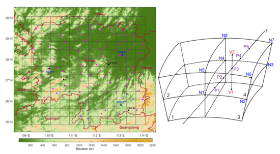
where is the wet refractivity, and is the propagation path of the signal through the troposphere. Given that the effect of a ray bending to SWD can be neglected for elevations greater than 15° [36], is usually taken as a straight line in the tomography. The model space is discretized into many voxels to reconstruct the wet refractivity field from the massive SWDs interweaving in the troposphere across different directions (Figure 1). The water vapor distribution is generally assumed to be homogeneous for each voxel over the reconstruction period. In this case, each SWD is approximately equal to the sum of the product of wet refractivity and the length of the ray path crossing each voxel. Therefore, Equation (2) can be approximated by:
where is the number of voxels along the SWD ray path, is the wet refractivity in voxel , and is the intercept of ray by voxel .
In the parameterized tomographic model, the wet refractivity of each voxel is no more regarded as invariable but varies with the position. The wet refractivity of a generic point is expressed by a weighted mean of the wet refractivity values at the 8 voxel nodes, where the point is located. For example, Figure 1 demonstrates that the wet refractivity of any point along P1–P5 can be determined from the 8 nodes (i.e., ) of voxel 4. Accordingly, the SWD can be expressed as an integral of the wet refractivities at the voxel nodes. The integral can hardly be analytically expressed; thus, the Newton–Cotes quadrature is used to solve the integral [33]. Figure 1 displays that the integral of wet refractivity along P1–P5 can be discretized as follows:
where is the intercept of ray by voxel 4; , , , , and are 5 equidistant points on the intercept; and the 4 constant values (i.e., 90, 7, 32, and 12) are coefficients for the 4-order Newton–Cotes quadrature formula. Perler et al. [33] adopted trilinear and bilinear/spline functions to interpolate the wet refractivity of point . In this work, an improved parameterization method was developed by considering the characteristic of the water vapor changes. The wet refractivity vertically follows the exponential distribution [8], thus taking as an instance, and its wet refractivity can be vertically interpolated by using points and :
where , , and refer to the altitudes of points , , and , respectively; and is a parameter describing the exponential variation of the wet refractivity, and it can be estimated from the following expression:
where represents the elevation of the lower surface of the vertical layer, and represents the elevation of a generic point within the layer. Variable is estimated for each voxel by using the wet refractivity profiles of the last tomographic period to improve the modeling performance. The initial profiles are derived from the National Centers for Environmental Prediction (NCEP) FNL Analysis products.
The wet refractivities of and are determined by the IDW interpolation:
where is the distance between and ; is the power of the distance; and represent the 4 neighboring voxel nodes of the grid surface, where point is located. For example, Figure 1 shows that the 4 surrounding nodes of point are , , , and . Here, we propose to estimate for each tomographic process to refine the modeling. In each voxel layer, is estimated from Equation (7) by using the wet refractivity field of the last tomographic period.
A large sparse system of linear equations is established by collecting all the SWD measurements over the tomographic period (30 min in this study):
where is a column vector with a set of SWDs, is the unknown parameter vector that consists of the wet refractivities of all voxel nodes, and is a matrix with elements denoting the contributions of on the SWDs. An inversion algorithm should be carried out to solve the unknowns. However, not all the voxels have ray crossings in most cases; thus, design matrix in Equation (8) is a large sparse matrix. To overcome the problem of ill-posedness, the horizontal and vertical constraints were imposed to regularize the linear least-square inversion. These constraints were added according to Equations (4) and (6). The a priori wet refractivity field provided by the National Centers for Environmental Prediction Final (NCEP FNL) analysis dataset was used to constrain the solution. The Helmert variance component estimation method was adopted to determine the weight of the a priori information for the tomographic solution [8].
However, the tomographic solution obtained from Equation (8) was just an approximate wet refractivity field. We thus further implemented the multiplicative algebraic reconstruction technique (MART) to improve the least square solution from Equation (8) due to its advantage of converging to a good result within a short processing time [16,32]. In the th MART iteration, the ratio between the observed y and reconstructed is computed to produce corrections for involved voxel nodes. Given the generic th ray and the generic th voxel node, the wet refractivity after the th iteration is calculated as follows:
where is the relaxation parameter (an empirical value of 0.9 used here). The wet refractivity field solved by Equation (8) was used as the initial for the iteration. The iteration was terminated when the standard deviation of the differences between GNSS-estimated and tomographically reconstructed SWDs was less than 0.5 mm. For cases the MART solution was unable to converge to 0.5 mm, the maximum iterations were set to 50. An accurate wet refractivity field will be obtained after performing the combined reconstruction algorithm [30,36,37,38]. Tomographic results solved from the parameterized method were wet refractivities of the voxel nodes. The vertical interpolation in Equation (5) and horizontal interpolation in Equation (7) must be implemented using the wet refractivities of the 8 voxel nodes of that voxel to obtain the wet refractivity of a generic point within a voxel. In the traditional tomography, the wet refractivity of a generic point is equal to that of its located voxel.
3. Validation of the Improved Parameterized Tomography
3.1. Experiment Description and Voxel Discretization
Various tests have been conducted to validate the performance of the proposed improved parameterized tomographic model. The tomographic experiment is carried out based on GPS observations collected from 124 stations with an average separation distance of 41 km (Figure 2) from the CORS network of Hunan Province, China. The time span of the GPS data used in the tests was from 1 to 30 June 2018, which is the most humid month in that year in Hunan. Tomography was consecutively implemented with an interval of 30 min. The SWDs from HNRC (113.34°E, 25.54°N, 499.061 m), SYDK (110.61°E, 27.03°N, 321.878 m), and XTXX (112.51°E, 27.75°N, 70.008 m) stations (black triangles shown in Figure 2) were excluded in the input dataset; they were used for self-consistency validation purposes. Most GPS stations were equipped with Trimble or Leica receivers and had a typical sampling rate of 30 s. In this work, Bernese 5.2 software was exploited to estimate the ZTDs with the PPP technique [39]. The ZTDs and horizontal gradients were estimated every 30 min and 12 h, respectively, while the global mapping function (GMF) was adopted [40] in the estimation. The comparison with radiosonde measurements revealed an accuracy of ~9 mm for our estimated ZTDs [41]. The quality-assured atmospheric profiles observed at 3 radiosonde stations (blue diamonds in Figure 2) from the Integrated Global Radiosonde Archive (IGRA) [42] will be used to validate the tomographic solutions.
The tomographic region covered from 108.85°E–114.05°E in longitude and 24.85°N–30.05°N in latitude. Radiosonde profiles revealed that wet refractivities approached zero at the altitude of 11 km. Therefore, the selection of 11 km as the top boundary of the tomographic region in Hunan and regarding the atmosphere above 11 km as dry air was reasonable. The water vapor variations in the latitude and longitude directions were comparable; thus, a uniform resolution of 0.4° in the 2 horizontal directions was adopted. The water vapor content rapidly decreased with altitude and was negligible in the upper troposphere. Considering the quasi-exponential behavior of the wet refractivity profile, we derived the following expression to determine the vertical layer distribution:
where denotes the altitude of the upper boundary of layer number , is the total number of vertical layers, is the minimal surface altitude within the target area, is the top height of the tomographic region, and is the exponential variation parameter that can be determined using (6) with history radiosonde data. Within the bottom and uppermost layer, this expression was established to distribute the intermediate layers for ensuring that the integral of the wet refractivity (i.e., ZWD) in each layer was approximately constant.
In this study, and were set as 0 and 11 km, respectively. A value of −0.28 was estimated for by using the historical radiosonde profiles collected over the whole month of June 2017. Flores et al. [11] suggested that the thickness of a vertical layer should be more than 350 m; otherwise, the noise will affect the tomographic solutions. Accordingly, the total number of layers was determined as 10 to ensure that the thickness of the lowest layer was larger than 350 m. Finally, 10 nonuniform layers were discretized with their thicknesses of 358, 398, 448, 513, 598, 719, 902, 1209, 1842, and 4013 m. The SWDs with elevation angles <10° were rejected in the tomography to minimize the multipath effects. Three schemes were used in the tomographic modeling to assess the performance of the improved method.
Tomo-I: Using the traditional nonparametric method that water vapor was assumed to have a homogeneous distribution within each voxel.
Tomo-II: Using the trilinear parameterization method developed in Perler et al. [33]. The bilinear/spline approach was not included here since it has a worse performance than the trilinear one in the assessment with real data. The wet refractivity at a generic point within a voxel was determined by trilinear interpolation from the wet refractivities at the 8 nodes of that voxel.
Tomo-III: Using the improved parameterized method developed in this study. As previously stated, the wet refractivity of any point within a voxel was expressed via vertical exponential interpolation and horizontal IDW interpolation by using the 8 refractivity values of the voxel corners.
3.2. Self-Consistency Validation by GPS Data
As previously mentioned, 3 GPS stations (i.e., HNRC, SYDK, and XTXX) were excluded from the tomographic experiment; however, they were adopted for self-consistency validation. The SWD along a generic ray path was calculated by an integral of wet refractivities with respect to its propagation path by using the tomographic results. The tomographic SWDs were then directly compared with those estimated from GPS measurements. Figure 3 exhibits the overall statistical results derived from the 3 stations during the period of 1–30 June 2018. The SWD derived from Tomo-I performed badly because its root mean square (RMS) error of 24.68 mm was approximately twice those of schemes Tomo-II and Tomo-III. With regard to the mean bias, the 3 schemes consistently yielded positive values in the range of 1.50 to 3.50 mm. This phenomenon was likely due to the neglect of the troposphere above altitude 11 km in the tomographic model as GPS-derived SWDs contained a small portion from the space above 11 km. RMS errors obtained from both the parameterized schemes were much smaller than the nonparametric scheme. The improvements attained by the parameterized method were 49% and 54% for schemes Tomo-II and Tomo-III, respectively. Tomo-III achieved the best performance with an RMS error of 11.40 mm, which corresponds to an improvement of approximately 10% with respect to Tomo-II.
Figure 4a shows the RMS errors of the SWD comparison at 8 different elevation intervals. The RMS errors quickly decreased with the increase in elevation in all comparisons. The RMS errors of the SWD differences for elevations between 10° and 20° were 2.7, 4.0, and 4.5 times those for elevations 80°–90° for Tomo-I, Tomo-II, and Tomo-III, respectively. The significant increase of the RMS error with elevation decrease occurred because the GPS rays will cost a longer time to travel through the troposphere at a low elevation, thereby leading to a larger wet delay. For this reason, Figure 4b further displays the change of relative RMS with elevations. The relative RMS was defined as the averaged GPS-estimated SWD divided by the corresponding RMS error. Tomo-I obtained relative RMS varying from 3% to 5%, whilst much smaller relative RMS values in the range of 1.5% to 2% were yielded for parameterized methods Tomo-II and Tomo-III. The relative RMS of Tomo-I, in general, increased with the elevation increase; however, slight decreases were found for Tomo-II and Tomo-III. This finding shows that the parameterized method was more robust than the traditional one because no evident changes in performance were observed at different elevations. Table 1 further illustrates the respective statistics of the reconstructed SWDs by the 3 schemes at the 3 GPS stations. Consistent with the overall statistics, Tomo-III performed best at all the stations, followed by Tomo-II.
3.3. Validation of the Tomographic Solutions by Radiosonde Profiles
Although the tomographic SWDs were in agreement with the GPS-estimated ones, the vertical profiles of wet refractivity were not necessarily correctly modeled. In this section, we further exploit radiosonde data to assess the tomographic wet refractivity profiles. Figure 2 shows that 3 radiosonde stations were located in Hunan Province. However, only 2 stations (i.e., RSCZ and RSHH) can provide observations for the period of the tomographic experiment. The measured radiosonde and the reconstructed tomographic wet refractivity profiles were resampled to heights with an interval of 200 m to conduct a straightforward comparison. In the traditional method, the wet refractivity of an arbitrary point was equal to that of the voxel where the point was located. The matchup wet refractivities of the parameterized methods were obtained by two steps: (1) Searching the voxel where the point was located; and (2) interpolating the wet refractivities of the 8 voxel nodes to the point by trilinear interpolation for Tomo-II or exponential/IDW interpolation for Tomo-III. The comparison between radiosonde and Tomo-I yielded a bias of 0.69 mm/km and an RMS error of 10.17 mm/km, respectively. The bias and RMS error of the wet refractivity profiles for Tomo-II were 0.27 and 7.81 mm/km, respectively. In scheme Tomo-III, the obtained bias and RMS error were −0.33 and 7.00 mm/km, respectively. The overall statistics showed that the tomographic profiles by Tomo-III have a great agreement with those observed by the radiosonde.
Figure 5 exhibits the change of RMS errors and relative RMS at various altitudes. Here, the relative RMS was defined as the averaged radiosonde-observed wet refractivity divided by the corresponding RMS of the layer. Tomo-III consistently showed the optimal performance with the RMS error decrease from ~10 mm/km at the bottom layers (0–1 km) to ~3 mm/km at the upper layers (9–11 km). The RMS errors of Tomo-I were larger than those of Tomo-II at various altitudes, particularly exceeding 30 mm/km at the bottommost layer. The relative RMS values for Tomo-III increased from 8% at the lowest layer to 443% at the uppermost layer with altitude. Figure 5b demonstrated that the relative RMS exceeded 100% at an altitude above 8 km for all the schemes. In the worst scheme Tomo-I, the relative RMS approached 1100% at the uppermost layer. This finding indicates the difficulty of tomography in reconstructing water vapor profiles of high-altitude layers. The water vapor content in the upper layers is small, and a minor error in the tomographic modeling would cause relatively large discrepancies in wet refractivity for the top layers.
3.4. Comparison of the Wet Refractivity Fields between Tomography and ERA5 Reanalysis
The limited spatial coverage of the benchmark datasets of the above 2 assessments hampered the comprehensive understanding of the tomographic solutions. ERA5 was the latest (5th generation) European Centre for Medium-Range Weather Forecasts atmospheric reanalyses of the global climate, which will replace its predecessor ERA-Interim within several years [43]. ERA5 reanalysis has been greatly upgraded in the spatiotemporal resolution and assimilation method compared with ERA-Interim [44]. ERA5 can provide hourly atmospheric parameters at 37 pressure levels from 1000 to 0.1 hPa at horizontal grids of 0.25° × 0.25°. ERA5 reanalysis offers us a chance to assess our tomographic solutions from the perspective of high spatial and temporal resolutions. Tomo-I, Tomo-II, and Tomo-III yielded biases of 3.27, 3.67, and 2.79 mm/km, respectively, by stacking 1-month comparison data of all voxels. The RMS errors of 10.79, 9.73, and 8.94 mm/km were obtained for Tomo-I, Tomo-II, and Tomo-III, respectively. Tomo-III had the optimal overall agreement with ERA5 data.
Figure 6a–c present the spatial distribution of the RMS errors of the wet refractivity differences between ERA5 and tomography over the study region. At each horizontal grid, the RMS error was calculated considering all the vertical voxels over this grid. The RMS errors of Tomo-I, Tomo-II, and Tomo-III varied from 7.0 mm/km to 16.8 mm/km, 5.9 mm/km to 15.8 mm/km, and 6.0 mm/km to 11.0 mm/km, respectively, depending on the location. In Tomo-I, large RMS errors exceeding 15 mm/km occurred in the southeast portion of the study area. In Tomo-II, the north part of the study area achieved a worse performance with RMS errors greater than 12 mm/km, with reasons unknown. In Tomo-III, a majority of the area was populated with RMS errors less than 10 mm/km, thereby showing an evidently enhanced consistency with ERA5. Figure 6d–f display the RMS differences between each of the two schemes. Figure 6d exhibits that the RMS errors of Tomo-I are larger than those of Tomo-II in most regions, except for the north above 29°N where the RMS differences of −1 to −3 mm/km are found. Tomo-III significantly performed better than Tomo-I because positive RMS differences were observed in the vast majority of the study area (Figure 6e). In Figure 6f, positive values could be observed everywhere, thereby demonstrating the improvements brought by Tomo-III versus Tomo-II for the parameterized method. The large RMS errors occurred in the boundary regions as less GPS rays interweaved in the troposphere. The southwest consistently obtained relatively good performance in all the 3 schemes, while no GPS sites were located there. The tomographic solutions of voxels over the southwest were highly dependent on the initial information due to the lack of GPS ray crossings. In this study, the NCEP FNL analysis was used to provide the a priori water vapor fields for the tomography. The NCEP FNL analysis had a good consistency with the ERA5 reanalysis, thereby leading to a low RMS error in the southwest. Figure 7 further shows the RMS error and relative RMS at 10 vertical layers. The RMS errors basically decreased with the increase in altitude from ~20 mm/km at the bottom to ~5 mm/km at the top. The relative RMS values decreased from approximately 20% at the bottom to over 90% at the top. The Tomo-III again outperformed the other 2 schemes at various vertical layers.
4. Conclusion and Outlook
The water vapor within each voxel is assumed to have homogeneous distribution in the tomographic modeling, which is unreasonable for cases with coarse voxel discretization and highly variable water vapor changes in the space. The parameterization of voxels can reduce the effects of discretization. In this study, we presented an improved parameterized algorithm for tropospheric tomography and validated its superiority in several tests. In the improved algorithm, the wet refractivity of a generic point is expressed via vertical exponential interpolation and horizontal IDW interpolation by using the eight refractivity values at the voxel nodes in which the point is located. The parameters involved in exponential and IDW interpolation are dynamically estimated for each tomography by using the wet refractivity field of the last process. In addition, an optimal expression is derived to discretize the vertical layers of the tomographic model, considering the quasi-exponential behavior of the wet refractivity profile. Various tomographic tests were carried out using SWD measurements estimated from 124 GPS sites of Hunan, China, over the whole month of June of 2018 to examine the performance of the improved parameterized method. Tomographic tests using the traditional nonparametric model and parameterized model with trilinear interpolation were also performed for a straightforward comparison with the improved model.
The tomographic water vapor results were fully evaluated with independent datasets derived from GPS, radiosonde, and ERA5 reanalysis. All assessments demonstrated the better performance of the improved model over the nonparametric model and the trilinear parameterized model. In the assessment by GPS-inferred SWD measurements, the improved model outperformed the traditional model and the trilinear parameterized model by 54% and 10%, respectively. In the evaluation of the wet refractivity profiles by radiosonde, the improved model yielded an RMS error of 7.00 mm/km with respect to 10.17 and 7.81 mm/km for the traditional model and the trilinear parameterized model, respectively. The RMS error vertically decreases from ~10 mm/km at the lowest layers (0–1 km) to ~3 mm/km at the uppermost layers (9–11 km). The relative RMS values increase from 8% (from the bottom) to 443%. The improved model achieved an optimal consistency with ERA5 reanalysis data with an overall RMS error of 8.94 mm/km. The RMS errors of the refractivity differences between ERA5 and the improved model vary from 6.0 mm/km to 11.0 mm/km throughout the study area. In the vertical profiles, the relative RMS increases from ~20% at the bottom to ~90% at the altitude of 9 km. Both assessments of the vertical profiles by radiosonde and ERA5 reanalysis reveal the difficulty of tomography in the reconstructing wet refractivity of altitudes above 8 km because the relative RMS may reach up to 1000% in the uppermost layer.
The high-quality water vapor fields retrieved by the tomography have many application potentials (e.g., atmospheric research, rainfall monitoring and forecasting, and GNSS positioning). In our study, the improved voxel parameterization methods have been developed to refine the spatial modeling. Future work will focus on the parameterized tomographic modeling with high temporal resolution (e.g., 5 min). The improvement in the standard and precise point positioning brought by the tomographic SWDs will be examined. The assimilation of the tomographic refractivity fields into a numerical prediction model to enhance the capability of precipitation forecasting should be considered in the future.
Author Contributions
B.C. designed this study, developed the methodology, performed the analysis, and wrote the manuscript. P.X. offered constructive suggestions in conceiving the experiment. W.D., M.A., and J.T. provided guidance and helped polish the manuscript. All authors have read and agreed to the published version of the manuscript.
Funding
This work was supported by the National Natural Science Foundation of China (grant no. 41904032, 41904025), the Natural Science Foundation of Hunan Province, China (grant no. 2019JJ50764), the Research Grant for Specially Hired Associate Professor of Central South University (project no. 202045005), and the Opening Foundation of Hunan Engineering and Research Center of Natural Resource Investigation and Monitoring (project no. 2020-11).
Acknowledgments
We want to thank the National Oceanic and Atmospheric Administration (NOAA) for providing the IGRA radiosonde data. The European Centre for Medium-Range Weather Forecasts is appreciated for contributing the ERA5 reanalysis data. The Hunan Province Mapping and Science and Technology Investigation Institute is grateful to provide the GPS observations of Hunan network. Finally, the authors want to thank the National Centers for Environmental Prediction/National Weather Service/NOAA/U.S. Department of Commerce for providing the NCEP FNL dataset.
Conflicts of Interest
The authors declare no conflict of interest.
Abbreviations
The following abbreviations are used in this manuscript:
| ECMWF | European Centre for Medium-Range Weather Forecasts |
| ERA5 | ECMWF ReAnalysis 5 |
| GNSS | Global Navigation Satellite System |
| GPS | Global Positioning System |
| GMF | Global Mapping Function |
| IDW | Inverse Distance Weighted |
| IGRA | Integrated Global Radiosonde Archive |
| MART | Multiplicative Algebraic Reconstruction Technique |
| NWP | Numerical Prediction Model |
| NCEP | National Centers for Environmental Prediction |
| NCEP FNL | NCEP Final |
| PPP | Precise Point Positioning |
| RMS | Root Mean Square |
| SWD | Slant Wet Delay |
| ZHD | Zenith Hydrostatic Delay |
| ZTD | Zenith Tropospheric Delay |
| ZWD | Zenith Wet Delay |
References
- Held, I.M.; Soden, B.J. Robust responses of the hydrological cycle to global warming. J. Clim. 2006, 19, 5686–5699. [Google Scholar]
- Chen, B.; Dai, W.; Liu, Z.; Wu, L.; Xia, P. Assessments of GMI-Derived Precipitable Water Vapor Products over the South and East China Seas Using Radiosonde and GNSS. Adv. Meteorol. 2018, 2018, 1–12. [Google Scholar] [CrossRef]
- Chen, B.; Liu, Z. Global Water Vapor Variability and Trend from the Latest 36-Year (1979 to 2014) Data of ECMWF and NCEP Reanalyses, Radiosonde, GPS and Microwave Satellite. J. Geophys. Res. Atmos. 2016, 121, 11442–11462. [Google Scholar] [CrossRef]
- Niell, A.E.; Coster, A.J.; Solheim, F.S.; Mendes, V.B.; Toor, P.C.; Langley, R.B.; Upham, C.A. Comparison of Measurements of Atmospheric Wet Delay by Radiosonde, Water Vapor Radiometer, GPS, and VLBI. J. Atmos. Ocean. Technol. 2001, 18, 830–850. [Google Scholar]
- Perler, D. Water Vapor Tomography Using Global Navigation Satellite Systems; Eidgenössische Technische Hochschule (ETH) Zürich: Zürich, Switzerland, 2012. [Google Scholar]
- Jacob, D.; Bärring, L.; Christensen, O.B.; Christensen, J.H.; Castro, M.; Déqué, M.; Giorgi, F.; Hagemann, S.; Hirschi, M.; Jones, R.; et al. An inter-comparison of regional climate models for Europe: Model performance in present-day climate. Clim. Chang. 2007, 81, 31–52. [Google Scholar] [CrossRef]
- Falconer, R.; Cobby, D.; Smyth, P.; Astle, G.; Dent, J.; Golding, B. Pluvial flooding: New approaches in flood warning, mapping and risk management. J. Flood Risk Manag. 2009, 2, 198–208. [Google Scholar]
- Chen, B.; Liu, Z. Assessing the performance of troposphere tomographic modeling using multi-source water vapor data during Hong Kong’s rainy season from May to October 2013. Atmos. Meas. Tech. 2016, 9, 5249–5263. [Google Scholar] [CrossRef] [Green Version]
- Rocken, C.; Van Hove, T.; Ware, R. Near real-time GPS sensing of atmospheric water vapor. Geophys. Res. Lett. 1997, 24, 3221–3224. [Google Scholar]
- Lee, S.; Kouba, J.; Schutz, B.; Kim, D.H.; Lee, Y.J. Monitoring precipitable water vapor in real-time using global navigation satellite systems. J. Geod. 2013, 87, 923–934. [Google Scholar] [CrossRef]
- Flores, A.; Ruffini, G.; Rius, A. 4D tropospheric tomography using GPS slant wet delays. Ann. Geophys. 2000, 18, 223–234. [Google Scholar]
- Rohm, W.; Bosy, J. The verification of GNSS tropospheric tomography model in a mountainous area. Adv. Space Res. 2011, 47, 1721–1730. [Google Scholar] [CrossRef]
- Rohm, W.; Zhang, K.; Bosy, J. Limited constraint, robust Kalman filtering for GNSS troposphere tomography. Atmos. Meas. Tech. 2014, 7, 1475–1486. [Google Scholar] [CrossRef] [Green Version]
- Bender, M.; Stosius, R.; Zus, F.; Dick, G.; Wickert, J.; Raabe, A. GNSS water vapour tomography—Expected improvements by combining GPS, GLONASS and Galileo observations. Adv. Space Res. 2011, 47, 886–897. [Google Scholar] [CrossRef]
- Yao, Y.; Zhao, Q. Maximally Using GPS Observation for Water Vapor Tomography. IEEE Trans. Geosci. Remote Sens. 2016, 54, 7185–7196. [Google Scholar] [CrossRef]
- Chen, B.; Liu, Z. Voxel-optimized regional water vapor tomography and comparison with radiosonde and numerical weather model. J. Geod. 2014, 88, 691–703. [Google Scholar] [CrossRef]
- Bi, Y.; Mao, J.; Li, C. Preliminary Results of 4D water vapor tomography in theTroposphere Using GPS. Adv. Space Res. 2006, 23, 551–560. [Google Scholar]
- Rohm, W. The precision of humidity in GNSS tomography. Atmos. Res. 2012, 107, 69–75. [Google Scholar] [CrossRef]
- Bender, M.; Raabe, A. Preconditions to ground based GPS water vapour tomography. Ann. Geophys. 2007, 25, 1727–1734. [Google Scholar]
- Zhao, Q.; Yao, Y. An improved troposphere tomographic approach considering the signals coming from the side face of the tomographic area. Ann. Geophys. 2017, 35, 87–95. [Google Scholar] [CrossRef] [Green Version]
- Ding, N.; Zhang, S.B.; Wu, S.Q.; Wang, X.M.; Zhang, K.F. Adaptive Node Parameterization for Dynamic Determination of Boundaries and Nodes of GNSS Tomographic Models. J. Geophys. Res. Atmos. 2018, 123, 1990–2003. [Google Scholar] [CrossRef]
- Shangguan, M.; Bender, M.; Ramatschi, M.; Dick, G.; Wickert, J.; Raabe, A.; Galas, R. GPS tomography: Validation of reconstructed 3-D humidity fields with radiosonde profiles. Ann. Geophys. 2013, 31, 1491–1505. [Google Scholar] [CrossRef]
- Chen, X.; Su, Y.; Liao, J.; Shang, J.; Dong, T.; Wang, C.; Liu, W.; Zhou, G.; Liu, L. Detecting significant decreasing trends of land surface soil moisture in eastern China during the past three decades (1979–2010): China’s 32 Year Soil Moisture. J. Geophys. Res. Atmos. 2016, 121, 5177–5192. [Google Scholar] [CrossRef] [Green Version]
- Manning, T.; Zhang, K.; Rohm, W.; Choy, S.; Hurter, F. Detecting severe weather in Australia using GPS tomography. J. Glob. Position. Syst. 2012, 11, 58–70. [Google Scholar]
- Zhang, K.; Manning, T.; Wu, S.; Rohm, W.; Silcock, D.; Choy, S. Capturing the signature of severe weather events in Australia using GPS measurements. IEEE J. Sel. Top. Appl. Earth Obs. Remote Sens. 2015, 8, 1839–1847. [Google Scholar] [CrossRef]
- Yu, W.; Chen, B.; Dai, W.; Luo, X. Real-Time Precise Point Positioning Using Tomographic Wet Refractivity Fields. Remote Sens. 2018, 10, 928. [Google Scholar] [CrossRef] [Green Version]
- Trzcina, E.; Rohm, W. Estimation of 3D wet refractivity by tomography, combining GNSS and NWP data: First results from assimilation of wet refractivity into NWP. Q. J. R. Meteorol. Soc. 2019, 145, 1034–1051. [Google Scholar] [CrossRef]
- Troller, M. GPS Based Determination of the Integrated and Spatially Distributed Water Vapor in the Troposphere; Swiss Federal Insititute of Technology Zurich: Zurich, Switzerland, 2004. [Google Scholar]
- Rohm, W.; Bosy, J. Local tomography troposphere model over mountains area. Atmos. Res. 2009, 93, 777–783. [Google Scholar] [CrossRef]
- Xia, P.; Cai, C.; Liu, Z. GNSS troposphere tomography based on two-step reconstructions using GPS observations and COSMIC profiles. Ann. Geophys. 2013, 31, 1805–1815. [Google Scholar] [CrossRef] [Green Version]
- Ding, N.; Zhang, S.; Zhang, Q. New parameterized model for GPS water vapor tomography. Ann. Geophys. 2017, 35, 311–323. [Google Scholar] [CrossRef] [Green Version]
- Bender, M.; Dick, G.; Ge, M.; Deng, Z.; Wickert, J.; Kahle, H.-G.; Raabe, A.; Tetzlaff, G. Development of a GNSS water vapour tomography system using algebraic reconstruction techniques. Adv. Space Res. 2011, 47, 1704–1720. [Google Scholar] [CrossRef] [Green Version]
- Perler, D.; Geiger, A.; Hurter, F. 4D GPS water vapor tomography: New parameterized approaches. J. Geod. 2011, 85, 539–550. [Google Scholar] [CrossRef] [Green Version]
- Andersen, A.H.; Kak, A.C. Simultaneous Algebraic Reconstruction Technique (SART): A superior implementation of the ART algorithm. Ultrason. Imaging 1984, 6, 81–94. [Google Scholar]
- Chen, B.; Wu, L.; Dai, W.; Luo, X.; Xu, Y. A new parameterized approach for ionospheric tomography. GPS Solut. 2019, 23. [Google Scholar] [CrossRef] [Green Version]
- Jiang, P.; Ye, S.R.; Liu, Y.Y.; Zhang, J.J.; Xia, P.F. Near real-time water vapor tomography using ground-based GPS and meteorological data: Long-term experiment in Hong Kong. Ann. Geophys. 2014, 32, 911–923. [Google Scholar] [CrossRef] [Green Version]
- Notarpietro, R.; Cucca, M.; Gabella, M.; Venuti, G.; Perona, G. Tomographic reconstruction of wet and total refractivity fields from GNSS receiver networks. Adv. Space Res. 2011, 47, 898–912. [Google Scholar] [CrossRef]
- Wen, D.; Yuan, Y.; Ou, J.; Zhang, K.; Liu, K. A hybrid reconstruction algorithm for 3-D ionospheric tomography. IEEE Trans. Geosci. Remote Sens. 2008, 46, 1733–1739. [Google Scholar] [CrossRef] [Green Version]
- Dach, R.; Lutz, S.; Walser, P.; Fridez, P. Bernese GNSS Software Version 5.2; Astronomical Institute, University of Bern: Bern, Swizerland, 2015. [Google Scholar]
- Boehm, J.; Niell, A.; Tregoning, P.; Schuh, H. Global Mapping Function (GMF): A new empirical mapping function based on numerical weather model data. Geophys. Res. Lett. 2006, 33. [Google Scholar] [CrossRef] [Green Version]
- Chen, B.; Dai, W.; Liu, Z.; Wu, L.; Kuang, C.; Ao, M. Constructing a precipitable water vapor map from regional GNSS network observations without collocated meteorological data for weather forecasting. Atmos. Meas. Tech. 2018, 11, 5153–5166. [Google Scholar] [CrossRef] [Green Version]
- Durre, I.; Vose, R.S.; Wuertz, D.B. Overview of the integrated global radiosonde archive. J. Clim. 2006, 19, 53–68. [Google Scholar]
- Hersbach, H.; Dee, D. ERA5 reanalysis is in production. ECMWF Newslett. 2016, 147, 5–6. [Google Scholar]
- Zhang, W.; Zhang, H.; Liang, H.; Lou, Y.; Cai, Y.; Cao, Y.; Zhou, Y.; Liu, W. On the suitability of ERA5 in hourly GPS precipitable water vapor retrieval over China. J. Geod. 2019, 93, 1897–1909. [Google Scholar] [CrossRef]
Figure 1.
Schematic representation of voxel discretization for the tomographic model.

Figure 2.
Geographic distribution of global positioning system (GPS) (triangles) and radiosonde (blue diamonds) stations in Hunan Province, China. The black triangles represent the GPS stations used for self-validation. The gray grids indicate the voxel discretization in the horizontal directions.
Figure 2.
Geographic distribution of global positioning system (GPS) (triangles) and radiosonde (blue diamonds) stations in Hunan Province, China. The black triangles represent the GPS stations used for self-validation. The gray grids indicate the voxel discretization in the horizontal directions.

Figure 3.
Biases and root mean square (RMS) errors of the tomographic slant wet delays (SWDs) solved using schemes Tomo-I, Tomo-II, and Tomo-III.
Figure 3.
Biases and root mean square (RMS) errors of the tomographic slant wet delays (SWDs) solved using schemes Tomo-I, Tomo-II, and Tomo-III.

Figure 4.
Change of the (a) RMS errors and (b) relative RMS with elevation for slant wet delay (SWD) comparisons between GPS and tomography.
Figure 4.
Change of the (a) RMS errors and (b) relative RMS with elevation for slant wet delay (SWD) comparisons between GPS and tomography.

Figure 5.
(a) RMS errors and (b) relative RMS of the differences between the wet refractivity profiles derived from radiosonde and tomography on the different altitude layers.
Figure 5.
(a) RMS errors and (b) relative RMS of the differences between the wet refractivity profiles derived from radiosonde and tomography on the different altitude layers.

Figure 6.
Maps of the RMS error of the wet refractivity differences between ERA5 and (a) Tomo-I, (b) Tomo-II, and (c) Tomo-III over the study area. Maps of (d–f) are the RMS differences between Tomo-I and Tomo-II, Tomo-I and Tomo-III, and Tomo-II and Tomo-III, respectively. The purple triangles represent the GPS sites used in tomography.

Figure 7.
Changes of the (a) RMS error and (b) relative RMS of the wet refractivity differences between ERA5 and tomography at different vertical layers.
Figure 7.
Changes of the (a) RMS error and (b) relative RMS of the wet refractivity differences between ERA5 and tomography at different vertical layers.


Table 1.
Biases and RMS errors of the differences between GPS-estimated SWDs and tomographic SWDs using schemes Tomo-I, Tomo-II, and Tomo-III.
Table 1.
Biases and RMS errors of the differences between GPS-estimated SWDs and tomographic SWDs using schemes Tomo-I, Tomo-II, and Tomo-III.
| Station | Tomo-I | Tomo-II | Tomo-III | |||
|---|---|---|---|---|---|---|
| Bias (mm) | RMS (mm) | Bias (mm) | RMS (mm) | Bias (mm) | RMS (mm) | |
| HNRC | 5.20 | 24.37 | 0.82 | 12.33 | 2.87 | 11.24 |
| SYDK | 0.54 | 24.12 | 6.12 | 16.40 | 0.51 | 11.37 |
| XTXX | 4.50 | 25.49 | 0.68 | 9.16 | 0.86 | 9.06 |
© 2020 by the authors. Licensee MDPI, Basel, Switzerland. This article is an open access article distributed under the terms and conditions of the Creative Commons Attribution (CC BY) license (http://creativecommons.org/licenses/by/4.0/).
Share and Cite
MDPI and ACS Style
Chen, B.; Dai, W.; Xia, P.; Ao, M.; Tan, J. Reconstruction of Wet Refractivity Field Using an Improved Parameterized Tropospheric Tomographic Technique. Remote Sens. 2020, 12, 3034. https://doi.org/10.3390/rs12183034
AMA Style
Chen B, Dai W, Xia P, Ao M, Tan J. Reconstruction of Wet Refractivity Field Using an Improved Parameterized Tropospheric Tomographic Technique. Remote Sensing. 2020; 12(18):3034. https://doi.org/10.3390/rs12183034
Chicago/Turabian StyleChen, Biyan, Wujiao Dai, Pengfei Xia, Minsi Ao, and Jingshu Tan. 2020. "Reconstruction of Wet Refractivity Field Using an Improved Parameterized Tropospheric Tomographic Technique" Remote Sensing 12, no. 18: 3034. https://doi.org/10.3390/rs12183034
Note that from the first issue of 2016, this journal uses article numbers instead of page numbers. See further details here.