Road Extraction from Very-High-Resolution Remote Sensing Images via a Nested SE-Deeplab Model


1
Institute of Agricultural Remote Sensing and Information Technology Application, College of Environmental and Resource Sciences, Zhejiang University, Hangzhou 310058, China
2
Department of Regional and Urban Planning, College of Civil Engineering and Architecture, Zhejiang University, Hangzhou 310058, China
*
Author to whom correspondence should be addressed.
Remote Sens. 2020, 12(18), 2985; https://doi.org/10.3390/rs12182985
Submission received: 4 August 2020
/
Revised: 3 September 2020
/
Accepted: 11 September 2020
/
Published: 14 September 2020
Abstract
:Automatic road extraction from very-high-resolution remote sensing images has become a popular topic in a wide range of fields. Convolutional neural networks are often used for this purpose. However, many network models do not achieve satisfactory extraction results because of the elongated nature and varying sizes of roads in images. To improve the accuracy of road extraction, this paper proposes a deep learning model based on the structure of Deeplab v3. It incorporates squeeze-and-excitation (SE) module to apply weights to different feature channels, and performs multi-scale upsampling to preserve and fuse shallow and deep information. To solve the problems associated with unbalanced road samples in images, different loss functions and backbone network modules are tested in the model’s training process. Compared with cross entropy, dice loss can improve the performance of the model during training and prediction. The SE module is superior to ResNext and ResNet in improving the integrity of the extracted roads. Experimental results obtained using the Massachusetts Roads Dataset show that the proposed model (Nested SE-Deeplab) improves F1-Score by 2.4% and Intersection over Union by 2.0% compared with FC-DenseNet. The proposed model also achieves better segmentation accuracy in road extraction compared with other mainstream deep-learning models including Deeplab v3, SegNet, and UNet.

1. Introduction
The recent, continuously expanding use of remote-sensing big data [1,2,3] has made very-high-resolution (VHR) images a vital geographic information data source because of their wide coverage and high accuracy. Information on road networks extracted from these images will have broad applicability, including in navigation, cartography, urban planning, and monitoring of geographical conditions. Roads are important artificial ground objects that form the main body of modern transport infrastructure. Maps therefore feature them prominently. Roads also constitute basic data in geographic information systems, and so the prompt updating of road information can affect anything relying on these systems: for example, map drawing, route analysis, and emergency responses. The rapid current development of unmanned vehicles relies heavily on road network information being kept up to date, and VHR remote sensing images can provide convenient, reliable, and high-quality data to support this task [4]. The automatic extraction of roads from satellite images has received much global research attention.
Deep learning is widely used in environmental remote sensing, such as land use extraction, land cover change analysis [5,6], remote sensing image classification [7,8], and object detection [9,10,11]. The deep-learning models commonly used in road extraction are convolutional neural networks (CNNs) [12], whose network structure is often used for various computer-vision tasks, and semantic segmentation technology [13,14,15,16,17,18] is another area of great research interest in image interpretation. For example, a fully convolutional network (FCN) can classify images at the pixel level [19,20,21,22,23,24], and its multi-scale feature fusion structure improves the accuracy of image segmentation. Compared with the FCN structure, a SegNet structure uses the pooled index calculated in the maximum pooling step of the corresponding encoder in the decoder structure to perform a nonlinear upsampling step, which can save more memory space and there is no need to update parameters in the upsampling stage, and many improved deep-learning models are based on the SegNet structure [25,26,27,28,29,30]. In order to improve the use of feature information in images, the long connection structure of UNet is also widely used in image segmentation, and this structure achieves the fusion of multi-scale image information to improve segmentation performance. Various improved UNet models have been developed for use in a range of fields [31,32,33,34,35], and TreeUNet can extract features in terms of the sizes and shapes of the associated ground objects [36].
Recent research has developed deep-learning methods for road detection, and deep belief networks have been applied for the first time to the task of extracting roads from airborne remote sensing images [37]. Considering the particularity of remote sensing images, Yong et al. [38] built a model based on texture features and other auxiliary feature information to realize automatic road extraction from VHR remote sensing images [38]. Deep residual UNet has been proposed to simplify the training of a deep network model, and it can extract road features from remote sensing images with less parameters compared with original UNet model [39]. Wang et al. [40] built a dynamic tracking framework based on a deep CNN and finite state machine that improves the accuracy of road extraction from VHR images. Tao et al. [41] proposed a spatial information inference structure, which aimed at the problem of extracting the roads occluded by other objects in remote sensing images, and this structure can learn both the local and global structure information of roads; they improved the continuity and accuracy of road extraction compared with other models by using this structure. Alshehhi et al. [42] designed an improved single patch-based CNN structure to achieve the extraction of buildings and roads; in the post-processing stage, the extracted features by CNN can be combined with the low-level features of roads and buildings such as asymmetry and compactness of adjacent regions, which improved the accuracy and integrity of extraction tasks. Xie et al. [43] combined the efficient LinkNet with a Middle Block to develop a HsgNet model, which made use of global semantic information, long-distance spatial information and relationships, and information of different channels to improve the performances in roads extraction with fewer parameters compared with D-LinkNet. An important aspect of research on road detection is center line extraction, which is not limited to semantic segmentation. Tejenaki et al. [44] developed an automatic hierarchical method, which improves the continuity level road detection and extraction. Liu et al. [45] extracted reliable road sections using feature filtering of the road shape and a hole filling algorithm; they extracted the center line of the road based on the fast-moving automatic sub-pixel skeleton method, but the selection of the method’s parameters and thresholds needs to be manually determined by trial and error. When performing road detection and center line extraction, there is always a problem associated with propagation error. To solve this problem, Yang et al. [46] put forward a recursive CNN model based on UNet using an end-to-end deep-learning scheme, which improves the accuracy of road detection and center line extraction compared with original UNet model. Given the original structure of Deeplab v3 model, the effective information of images and feature maps is not well preserved and used in downsampling and upsampling. Pooling layers of Deeplab v3 have lost a part of image information in the encoder part [47,48], and the receptive field of encoder output is large, so multi-scale feature information in decoder structure is not made use of well. Therefore, when extracting road features of different sizes, some smaller targets in remote sensing images are often ignored, and the integrity of image segmentation is reduced because of the problems associated with a large receptive field and the features of long and thin roads. Making full use of the feature information in VHR images can greatly reduce the training pressure of the model while improving its testing efficiency and segmentation accuracy.
Here, we propose an improved Deeplab v3 model combined with SE module for extracting roads from VHR images in the Massachusetts Roads Dataset. The remainder of this paper is organized as follows: Section 2 introduces the research methods, including the dataset used in this paper, the detailed structure of the proposed model (Nested SE-Deeplab) and different selection of loss function and backbone networks. Section 3 introduces the experimental results of each comparative study, including different loss function, backbone modules, and comparison between Nested SE-Deeplab and other deep learning models. The discussion of methods and results is provided in Section 4. Finally, Section 5 concludes the work.
2. Materials and Methods
2.1. Dataset
The dataset used here is the Massachusetts Roads Dataset [49], which was established by Volodymyr Mnih. Remote sensing images of Massachusetts, USA are collected from this dataset, with their road parts labeled to generate annotated maps. A total of 697 images are used in this study, 604 for training, 66 for validation, and 27 testing. Each of the images is 24-bit, true color tiff image with the size of 1500*1500 pixels and a resolution of 1m/pixel. Each pixel in the annotated map is classified as either road or non-road. Figure 1 shows samples from the dataset.
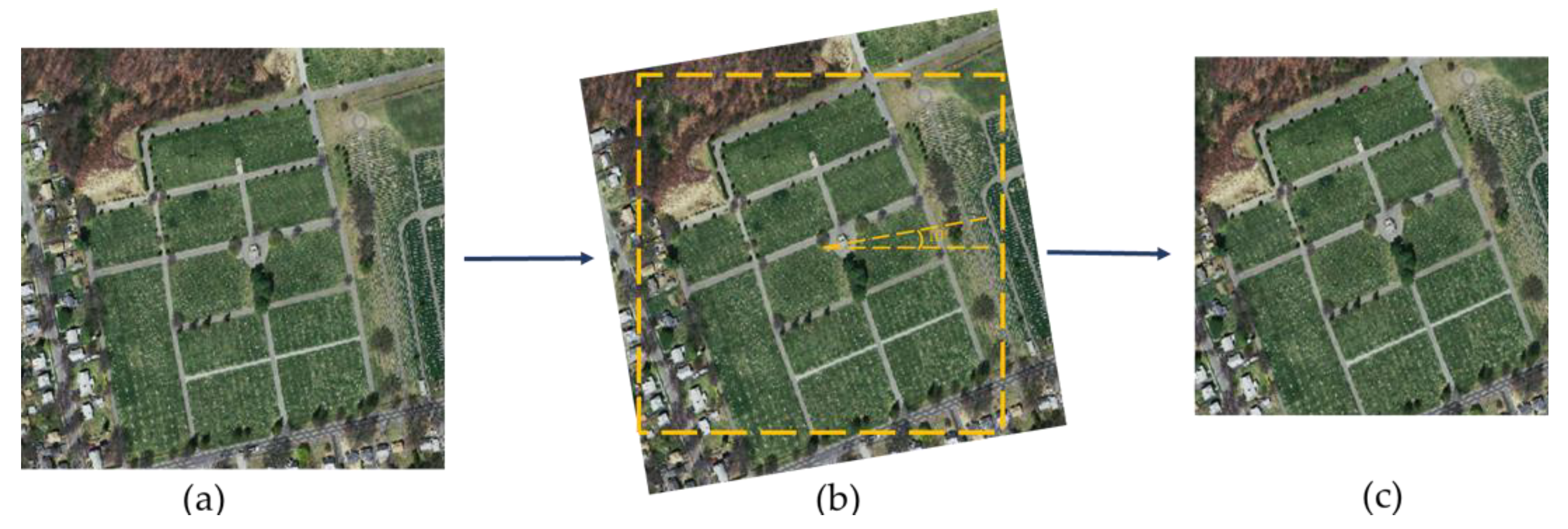
To enhance the generalizability of model prediction, data enhancement is applied by rotating and cropping the images before modeling. The original image and the annotated image are rotated 10° counterclockwise, and then cropped as shown in Figure 2. This increases the diversity of road parts in the image data, provides more features of road parts for model training, and therefore enhances the robustness of the model.
2.2. Nested SE-Deeplab
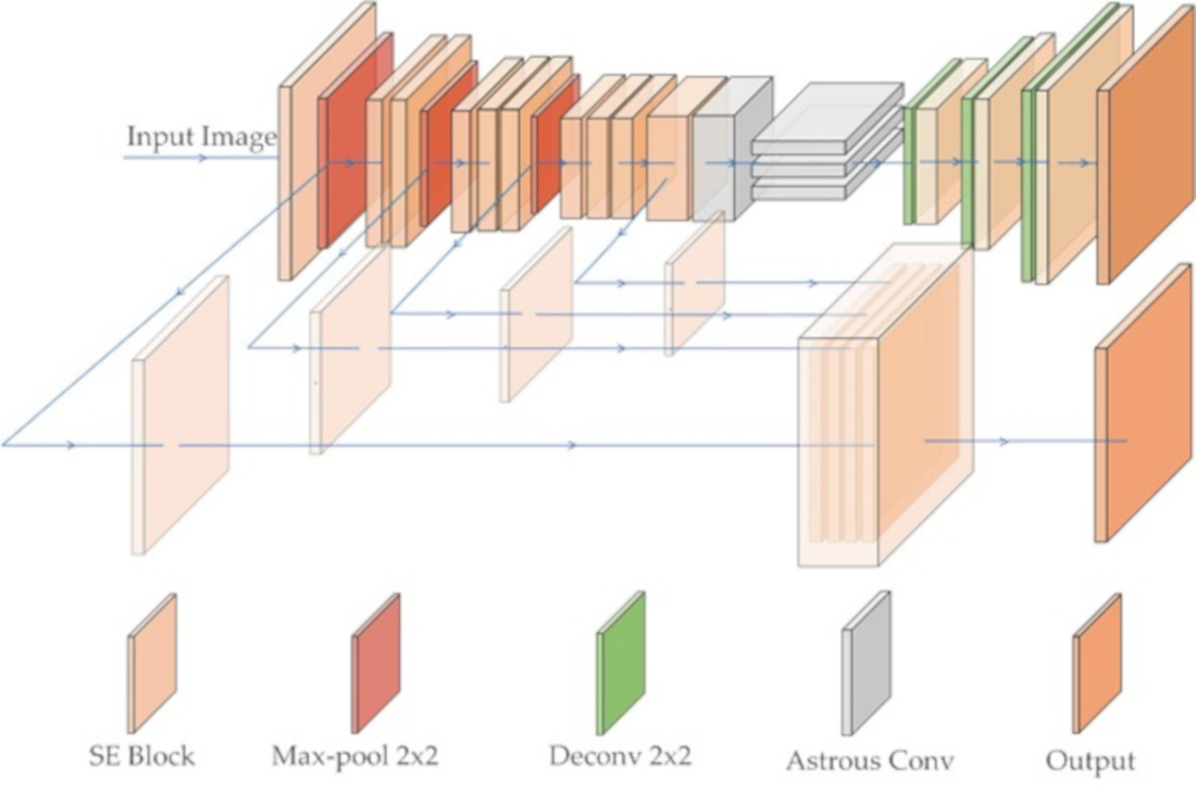
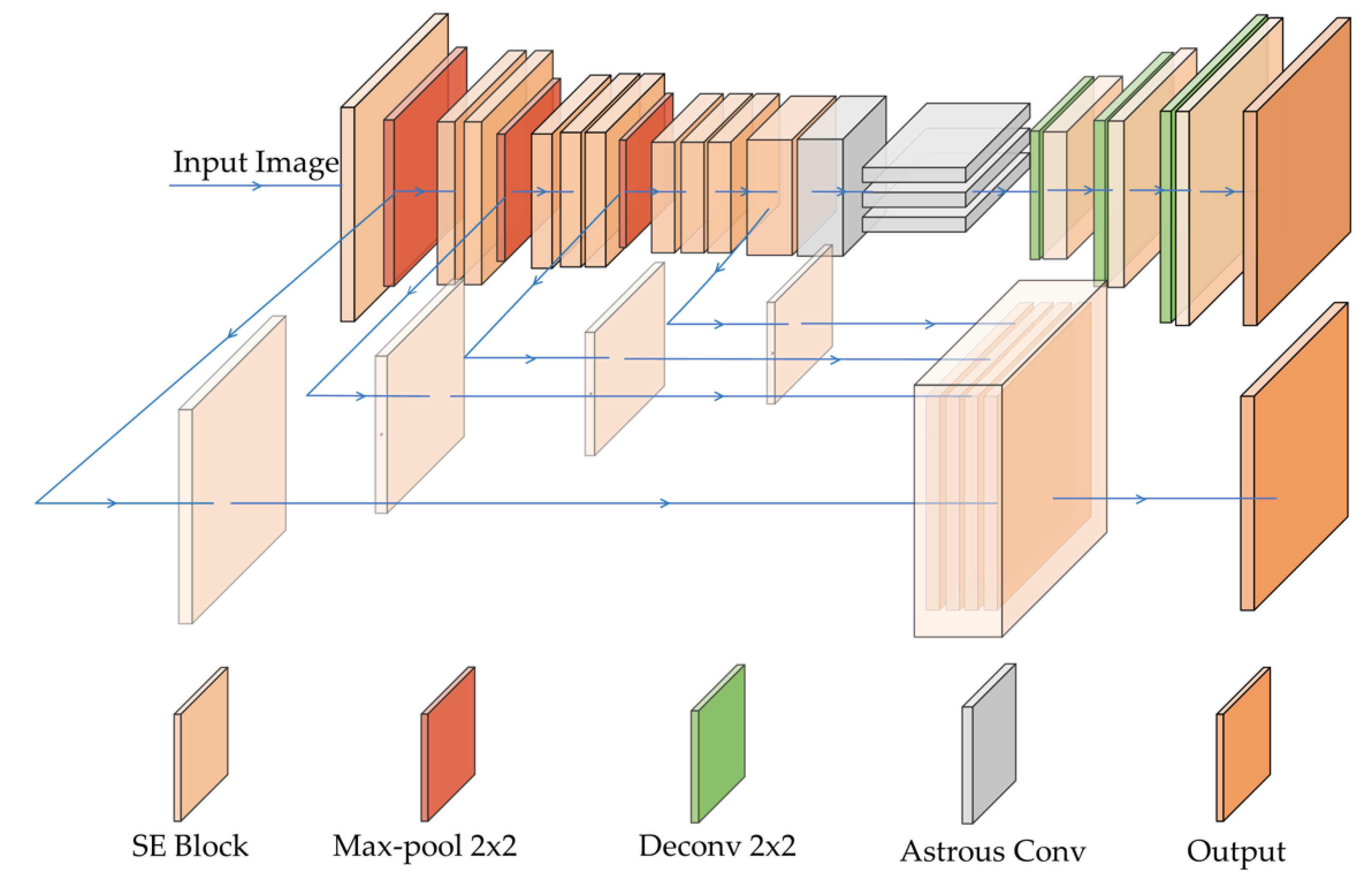
This paper proposes a deep model (Nested SE-Deeplab) for segmenting roads with different sizes in VHR remote sensing images. The structure of the model is based on Deeplab v3, with the original encoder and decoder structure reformed. It combines a SE module with a residual structure. The model mainly focuses on image information processing during prediction, and aims to effectively combine shallow and deep feature information. Compared with the original Deeplab v3, the proposed model can strengthen the important channel information and solve the problem of information loss in most CNN models. The following subsections introduce the structure and function of each part of the proposed model and the calculation process from input to output (Figure 3).
2.2.1. Squeeze-and-Excitation Module
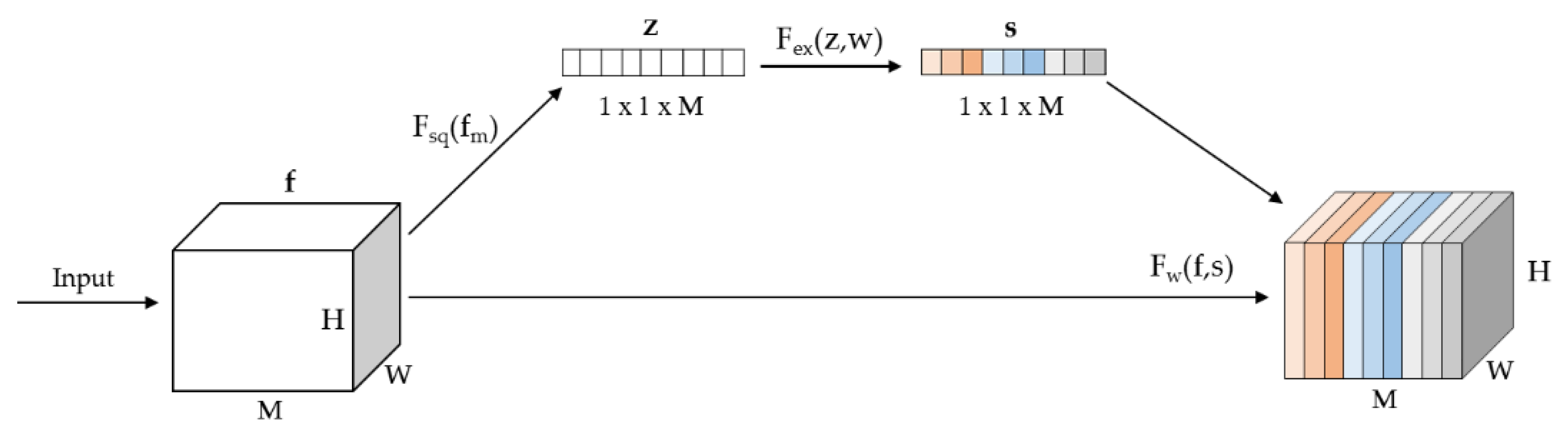
The SE module [50] considers the relationships among channels in the feature map and provides different weights for each channel. It automatically acquires the importance of each feature channel by model learning, and then strengthens useful features while suppressing those not useful to the current task according to the importance of each channel. The structure of the SE module is shown in Figure 4. Squeeze and excitement are two key operations in the SE module.
(1) The squeeze operation changes each two-dimensional feature channel into a real number by means of global average pooling. Its input and output have the same number of feature channels, and the real number has a corresponding global receptive field, which represents the spatial distribution of the corresponding features of this channel. The squeeze operation can be defined as:
where m is the index of the channel of the feature map, H is the number of the pixel of the feature map’s height, W is the number of the pixel of the width, fm is the value of the pixel whose index is (i, j) in the feature map.
(2) The excitation operation realizes the function of attention mechanism [51,52]. The process is defined by
where w including w1 and w2 is the weights in fully connected layers, δ is the ReLU function after the first fully connected layer, and σ is a sigmoid activation after the last layer to form the weights for the information of every channel.
The output of squeeze is normalized by a sigmoid function, and taken as the weight for each channel; it characterizes the correlation between each feature channel. This output can provide different weights for each channel by multiplication, and the feature information in different channels is either strengthened or suppressed. Finally, the input and output of the module are fused using a residual structure, which preserves shallow information in the original image and ensures the training depth of the model.
2.2.2. Model Encoder and Decoder
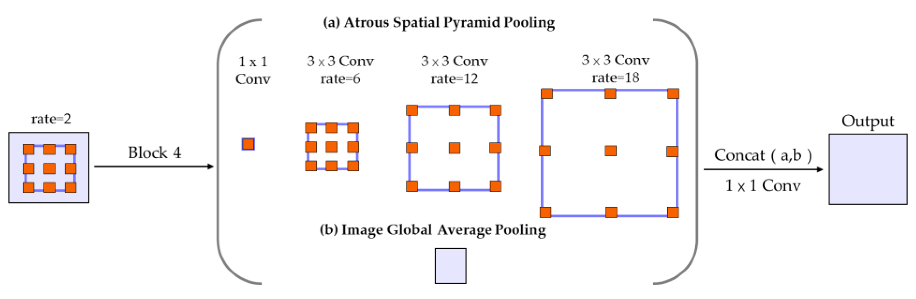
The original structure of Deeplab v3 contains atrous spatial pyramid pooling (ASPP) module [16] and four blocks with ResNet, and the output of the ASPP returns the original size by upsampling. The ASPP module is the key structure in Deeplab v3, which can explore the characteristics of different receptive fields and integrating them by atrous convolution and concat methods. The structure is shown in Figure 5. The atrous convolution in ASPP can retain more image information to improve the segmentation accuracy and increase receptive fields without pooling layers, and it can be defined as:
where y[n] is the output of the pixel whose index is n, k is the location index in kernels, r is the atrous rate that determines the size of convolution kernels and w is filters with weights. Atrous convolution kernels can be produced by inserting r−1 zeros between two weights in standard convolution kernels. Changing rates can adjust sizes of the receptive fields for different segmentation tasks.
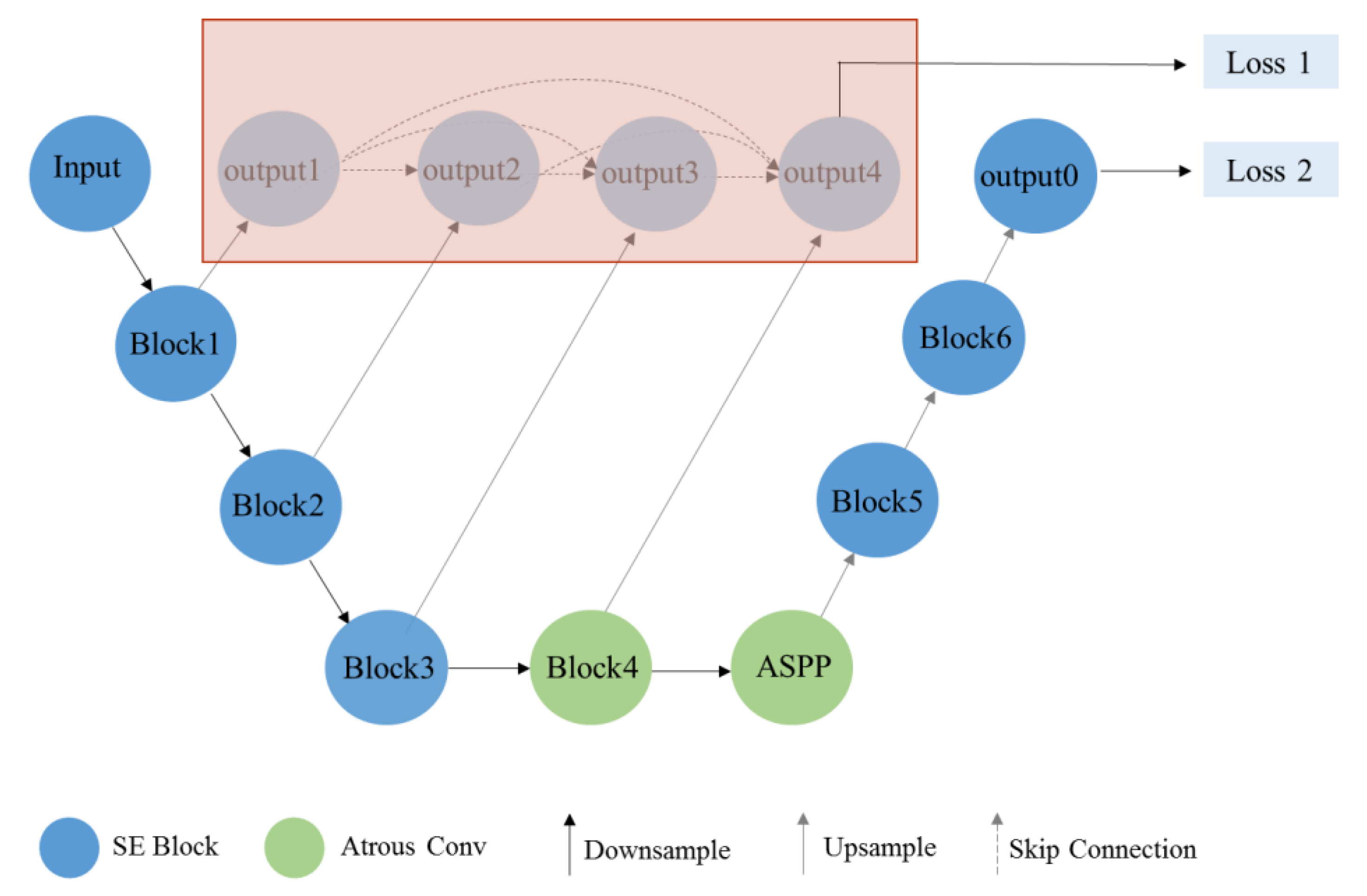
The proposed model has the structures of its encoder and decoder improved compared with those in Deeplab v3, so it can save and process image information better. In the encoder, after every downsampling step, the output of this layer will be upsampled, and the size of the feature map will be extended to the original size. Before the atrous spatial pyramid pooling (ASPP) module, the encoder carried out upsampling operations four times in total. The outputs obtained from the four upsampling steps are fused with feature information using channel concat. This output of the encoder is passed through a convolution layer to realize the function of deep supervision, and the final feature map is taken as one of the outputs of the model.
During different experimental stages including training, validation, and testing, the structure of the model is different. The structure in red in Figure 6 is needed in model’s training, and the structure in red region can be hidden without calculation during model’s validation and testing. During training, apart from the final output of the decoder, the encoder will produce an extra output, so the structure of the red region can also help the proposed model update the parameters of the encoder part. The output of this part fuses the information of various scales, which improves learning of the information of feature maps with different sizes. The structure in the red region can be discarded during validation and testing phase without affecting the final output of the model; this would reduce flops and improve the calculation efficiency. In the decoder, the proposed model upsamples the results obtained by ASPP several times, and combines the SE module with ResNet as backbone structure to get the final output layer-by-layer, which is then expanded to the original size. Compared with the structure of restoring to the original size only by one deconvolution layer, which is the decoder structure of Deeplab v3, the structure with multi-scale feature image fusion and layer-by-layer deconvolution can make better use of image information, thereby improving the model’s prediction accuracy.
2.2.3. Model Structure and Training
In the encoder, the SE module is added to the original backbone network of Deeplab v3, and SE-ResNet is taken as the baseline structure for the proposed model. Every time the model passes through a block, the number of feature channels is doubled, and the output of each block is upsampled to the original image size; these feature maps are fused by concat of channels to obtain one of the outputs of the model. After running the maximum pooling step and the fourth block, atrous convolution and ASPP structure consistent with Deeplab v3 are added. The decoder employs SE-ResNet as the backbone network to upsample the result of the encoder. After three upsampling steps in the decoder, the feature map is returned to the original image size as the second output of the model, and the two outputs of the encoder and decoder are fused as the final output during model training, which can achieve that the parameters of both shallow and deep layers can be trained better than original structure. Validation and testing can discard the calculations in the red region (upsampling in the encoder), which saves computing cost without affecting the accuracy of the model; only the encoder–decoder part is executed, and the model will eventually produce only one output which is the result of decoder.
2.3. Selection of Loss Functions
This study essentially considers a deep-learning task of binary classification, with the dataset only containing road information and non-road information. In addition, the proportions of the two classes in the dataset are different. The annotated map has far fewer road pixels than background pixels, so the positive and negative samples are unbalanced in the classification task. The loss function is an important part of measuring the relationship between predicted and true values. In a binary classification task, problems arising from having unbalanced numbers of the positive and negative classes can be reduced or avoided by selecting an appropriate loss function. Cross-entropy loss function has been widely used in building deep learning models. As the cross-entropy loss function evaluates the class prediction of each pixel vector and then averages all pixels, it can be considered that pixels have been learned equally; therefore, the effect of the loss function may worsen when the numbers of positive and negative samples are very unbalanced. Using the dice coefficient can avoid this problem. The dice-coefficient loss function focuses on the coincidence of the label and the prediction, which performs better for unbalanced samples compared with the cross-entropy loss function that focuses on the fitting level of all the pixels. However, dice loss is still sensitive to noise, and may ignore boundary information, resulting in poor boundary segmentation.
The proposed model uses four different loss functions to compare the segmentation results of VHR images. The considered loss functions are softmax cross entropy, weighted log loss, dice coefficient, and dice coefficient added with binary cross entropy (dice+bce).
(1) Softmax cross entropy has two steps, which can be defined as Equation (5). First, the output obtained by the model is processed by softmax for normalization, and the obtained class vectors are transformed into probability distribution vectors, so the output of each class corresponds to the probability of the corresponding class. Binary classification uses softmax and sigmoid functions for equivalence.
where yi is the real class of the pixel whose index is i, . the ith predicted result of the model, M is the number of classes, and N is the total number of pixels in the images as inputs.
(2) Weighted log loss uses weighted cross entropy to distribute sample weights when the positive and negative samples are unbalanced, so that the different samples can be weighted during prediction, reducing the influence of the unbalanced numbers of different categories. This loss function is shown in Equation (6):
where pi is predicted probability for the pixel, r is a weight given to balance the numbers of positive and negative samples.
(3) Dice coefficient defined as Equation (7) is derived from binary classification, which essentially measures the overlap of the predicted and real values. The index ranges from 0 to 1, where “1” means complete overlap and “0” means there is no area of overlap.
(4) dice+bce has binary cross entropy added to dice coefficient loss, and weighting these two loss functions is intended to solve the problem of an unbalanced sample distribution and improve the definition of road boundary extraction. The format of dice+bce is defined by
2.4. Selection of Backbone Networks and Modules
When a CNN is used to regress or classify targets, the gradient may disappear with the increase of network layers during training. This makes it impossible to update the parameters of the shallow network during back propagation, and the performance of the model consequently decreases. Therefore, the residual network is widely used in deep-learning models to solve the above-mentioned problem and retain more original information of feature maps [53,54]. In order to make better use of the effective information of feature maps, the attention mechanism structure can be selected to suppress the utilization of useless information and increase the weights of important information to improve prediction performance of models. Therefore, selecting appropriate backbone networks and modules can achieve segmentation tasks with better integrity.
The backbone networks used in this study are as follows. 1. ResNet block contains two or three convolutional layers. The output of the last convolutional layer has the same shape of feature maps as the input of the ResNet block, and the input is combined with the output through the residual structure to form the final output of the block. This structure solves the gradient disappearance problem caused by a deep network structure; the residual structure facilitates retention of original information through reducing information loss. 2. ResNext [55], in comparison with ResNet, has increased cardinality for a given level of layers, using a split-transform-merge strategy to improve generalization ability of the model, and shows improved network performance without increasing the depth or width of the network. 3. SE-Net, in comparison with other neural units, can build models in terms of the dependence between channels and adaptively adjust the characteristic response values of each channel: that is, it filters out the attention to each channel, and provides different weights to each channel for each layer, thus improving prediction performance.
2.5. Comparison with State-of-the-Art
To evaluate the performance of the proposed model for road extraction, it is compared with mainstream deep-learning models. The list of models used in this study includes following:
(1) Deeplab v3 is a deep-learning model using atrous convolution and multi-scale ASPP structure; it omits the pooling operation to increase retention of original information from the images.
(2) SegNet has a symmetric encoder–decoder structure based on the semantic segmentation structure of FCN; the corresponding pooled index is saved in the encoder, and index mapping is realized in the decoder. End-to-end pixel-level image segmentation is realized by an upsampling operation called unpooling.
(3) UNet is a network originally developed for biomedical image segmentation. The encoder and decoder are symmetrical in structure, and the feature maps of downsampling and upsampling are fused by skip connection and concat.
(4) FC-DenseNet has a U-shaped CNN structure constructed with dense connections, and feature maps at different levels are connected by concat to realize feature reuse.
(5) The Nested SE-Deeplab model proposed here fuses SE module and residual structure with Deeplab v3, preserves and fuses feature maps at different scales in the encoder, and produces two outputs that will be finally fused for training. The parameters (e.g., training environment, optimizer, loss function, and learning rate) are set to be the same in each network model. Road feature extraction results from previous research using the same dataset is also cited for comparison [49].
2.6. Parameter Settings
To increase the training efficiency of the model, unified processing of the input data for model training is required. Each original image and annotation map with 1500*1500 pixels is divided into some small batches of 100–200 randomly generated sub-images (with the size of 256*256 pixels and corresponding annotated maps) using any starting point in each original image. The sub-images are saved as arrays in TFRECORD files, which are taken as inputs to facilitate training. Table 1 lists the distribution of training, validation, and testing images and the numbers of corresponding sub-images.
The environment and framework used here are Python v3.6 [56], Tensorflow v1.14.0 [57], and Keras v2.1.2 [58]. Modeling process uses adaptive moment estimation to optimize the loss function. There are four samples in each iteration, and the initial learning rate is 1 × 10⁻⁵. For every 2000 iterations, the learning rate is adjusted by a factor of 0.98 (i.e., reduced by 2.0%). Attenuating the learning rate helps the loss function rapidly reach the local optimum. The hardware configuration is 64 GB memory, and the CPU is i7 9700 K and RTX2080ti GPU with 11 GB memory.
2.7. Evaluation Indexes
In this binary classification task, the proposed model and other mainstream deep-learning models are evaluated using overall accuracy, recall rate (correctness), F1-Score, and Intersection over Union (IoU). These evaluation indexes are defined by
where true positive (TP) represents the number of road pixels predicted successfully as the positive class, true negative (TN) represents the number of background pixels predicted successfully as the negative class, false negative (FN) represents the number of road pixels classified as background, and false positive (FP) represents the number of negative class pixels predicted as positive, which means background pixels classified as roads.
3. Results
3.1. Comparison of Loss Functions
This section examines the use of different loss functions in the proposed model, and compares the segmentation results of VHR remote sensing images based on different loss functions, with the goal of selecting the best one for use in subsequent research.
Figure 7 presents the segmentation results for the target roads achieved with the different loss functions. The magnifications in Figure 8 emphasize the differences between cross entropy and dice coefficient, although FNs consistently outnumber FPs in each case. The model with softmax cross entropy yields more FNs than the other loss functions. Using weighted log cross entropy does not offer a great improvement over softmax cross entropy, and there is still the loss of positive sample information. Compared with the cross-entropy loss function, the dice coefficient series improves the segmentation accuracy and integrity of road extraction under the condition of unbalanced samples. The dice coefficient is better than dice+bce in this experiment, and it achieves the lowest FN amount of all the tested loss functions. Overall, dice loss has the best integrity of road feature extraction. Table 2 summarizes evaluation indexes for the prediction results of the proposed model. The dice coefficient gives the best feature extraction for this dataset, as it achieves better integrity than the cross-entropy loss function in terms of F1-score and IoU.
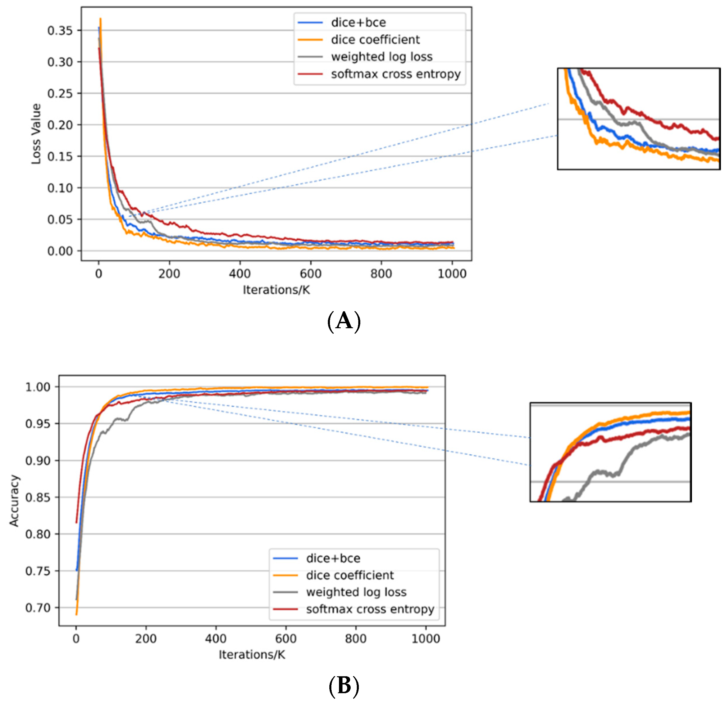
Figure 9 plots the changes in the loss value and training accuracy of the proposed model applied using the four different loss functions during training with respect to the number of iterations. The dice coefficient has loss stabilize the quickest, after which dice+bce, weighted log cross entropy, and softmax cross entropy converge in turn (Figure 9A). Comparison of the results after convergence shows dice coefficient and dice+bce having smaller loss values than the other functions. The maximum training accuracy of the four loss functions is similar, but for a given batch size and learning rate, dice coefficient and dice+bce reach the maximum training accuracy faster than softmax cross entropy and weighted log loss (Figure 9B). Therefore, the dice coefficient appears best for this dataset to improve the problem associated with an unbalanced numbers of the positive and negative samples.
3.2. Comparison of Backbone Networks
This section examines the use of different backbone networks and modules in the proposed model, and results obtained using the SE module are compared with those from other residual structures (ResNet and ResNext).
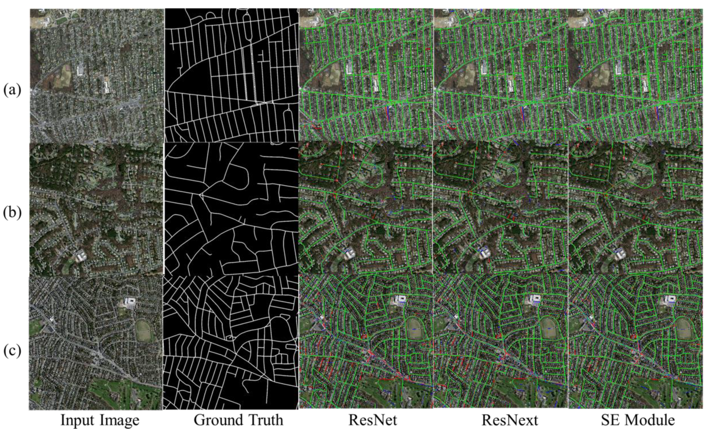
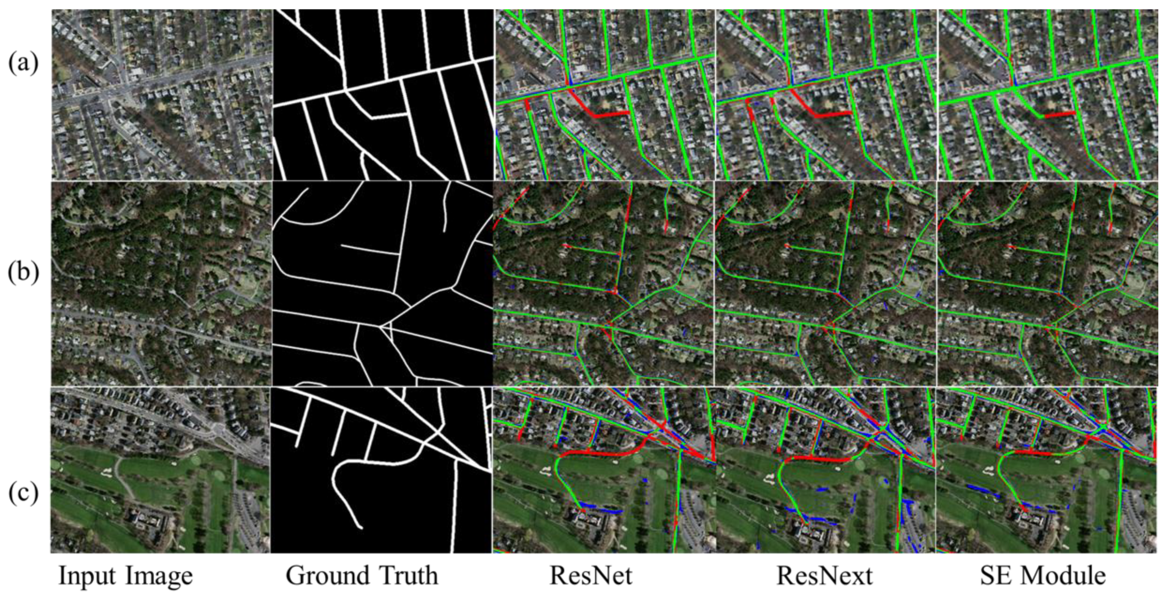
Figure 10 and Figure 11 visually compare road segmentation results from the three backbone network structures applied with the proposed model. The three structures achieve generally good results in VHR remote sensing road extraction. Compared with the ResNet originally used in Deeplab v3, ResNext and SE-Net show lower amounts of FN, and therefore better road segmentation. ResNet is not ideal for segmenting small targets such as some of the roads seen here, and there are some misclassification cases. All the structures fail to extract the complete road information. Compared with SE-Net, ResNext has more FPs (i.e., more background pixels misclassified as roads), and the proposed model added with SE module perform better in integrity of road extraction in this dataset. Overall, the SE-Net structure achieves the best road segmentation, showing fewer FNs and FPs than the other two structures.
Table 3 provides summary statistics on the three evaluation indexes of the model prediction results in this part. The SE module achieves the best road extraction, with better correctness, F1-score, and IoU values than the other backbone networks. This result is consistent with the first impression from Figure 10 and Figure 11, indicating that the SE module is a great improvement compared with ResNet originally used in Deeplab v3. ResNext shows the second best performance during testing. ResNet with single residual structure fails to make use of road information in images well and performs comparatively poorly in extracting complete road information, showing many misclassification cases.
3.3. Model Comparison
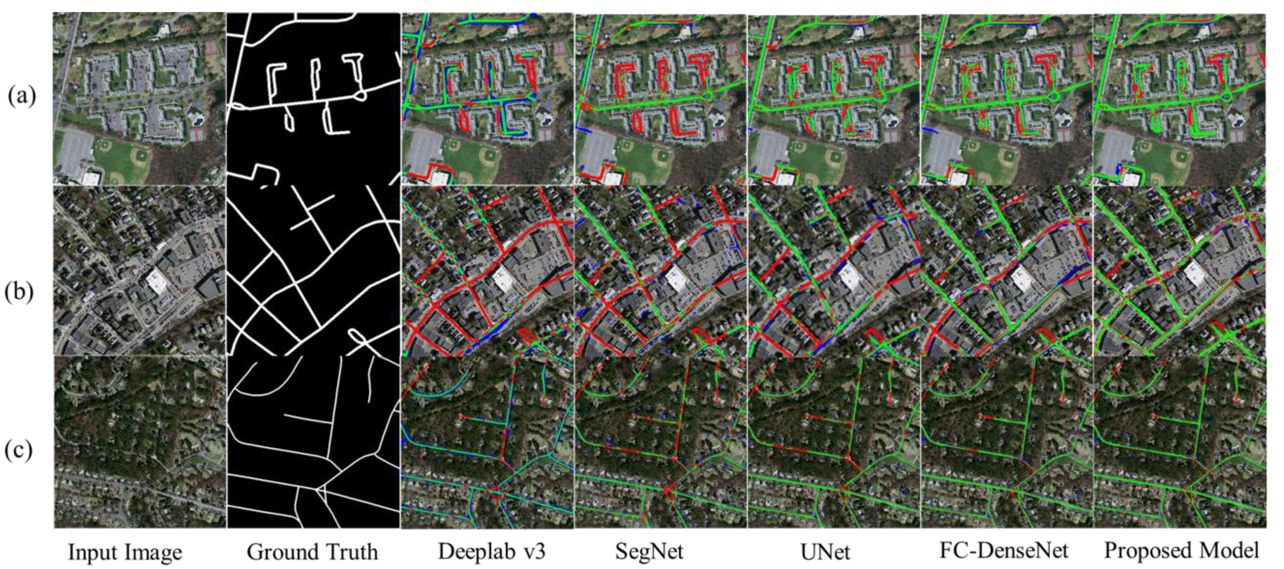
Figure 12 and Figure 13 depict the performance of the five deep-learning models for the testing dataset. The original Deeplab v3 and SegNet models perform poorly, with large amounts of FN and poor road integrity. Especially in the result of Deeplab v3, there are many discontinuous roads extracted in its segmentation results. UNet and FC-DenseNet perform better. Particularly, UNet has a long connection structure that can retain more information and improve the integrity of road segmentation. However, UNet and FC-DenseNet are not effective in extracting roads from dense distributions and small targets, and there are still many FNs and FPs. In comparison, the proposed model shows better extraction performance; it improves the integrity of road extraction and reduces FP misclassification. Although the proposed model still misses some road information when segmenting obscure roads in the images, it shows improved semantic segmentation in road extraction and better segmentation performance compared with the other models tested here.
Table 4 lists evaluation indexes for the prediction results of the different models. Among the five models tested here, the proposed model performs best in the testing dataset. Compared with the index values of FC-DenseNet, the proposed model yields an F1-score of ~2.4% higher, its IoU value is 2.0% higher, and the overall accuracy is 1.5% higher. With regard to the precision of road extraction, the performance of the proposed model is improved by 1.1% compared with ELU-SegNet-R [59]. The proposed method therefore shows improved segmentation performance for this dataset.
4. Discussion
In this study, road extraction from VHR remote sensing images is realized using an improved Deeplab v3 model, Nested SE-Deeplab. The results presented here show that, for the Massachusetts Roads Dataset, loss functions employing dice coefficient converge more quickly during training than those with cross entropy, and dice coefficient loss function has better training accuracy. They also lead to better prediction performance under the same parameter and environment settings than cross entropy. A cross-entropy loss function predicts each pixel as an independent sample, while the dice coefficient itself can be used as an index to evaluate a segmentation model. Compared with cross-entropy loss, the dice coefficient mainly measures the overlap between the prediction result and label, and calculates a loss value by taking all pixels of one class as a whole. During training, a segmentation index (e.g., IoU) is directly used as a loss function to supervise network training, and a large number of background pixels can be ignored when calculating the intersection ratio. Our comparative study of four different loss functions shows that the proposed model using dice coefficient performs better than that with dice+bce. Dice+bce can improve the performance of a model when samples have balanced amounts of data in each class. However, for the unbalanced situation of this dataset used here, as the number of iterations increases, the value of binary cross entropy will become much smaller than dice loss, which could affect the performance. Although this paper compares different loss functions to evaluate road extraction from unbalanced samples, the structure of the loss function is not improved according to the features of the roads. In further study, we can attempt to construct a loss function for road extraction according to the morphological characteristics of roads in remote sensing images, which is more targeted for road extraction during building models.
To improve the integrity of road extraction, the choice of backbone network is also considered here. Our results show that ResNext is better than ResNet for this road segmentation task. Except for the residual structure, it uses packet convolution without changing the width and depth of the network, and the feature maps obtained by different convolution paths have lower coupling than those from ResNet. ResNext’s different cardinality from ResNet’s aims at different image features, so it can complement and supplement the feature map information, therefore improving the integrity of the model in road extraction. Compared with ResNet and ResNext, the proposed model with a SE module better extracts roads from this dataset. The SE module contains the structure of an attention mechanism. During road extraction, the SE module can strengthen the information contained in important channels, and give smaller weights to channels with weak prediction function. It saves more original road information through the residual structure to ensure depth during training, which can improve the training efficiency and prediction accuracy, and thus increase the integrity of the extracted roads.
Compared with UNet and Deeplab v3, the proposed model has improved encoder and decoder structures. The output of each downsampling is given the operation of upsampling to the original image size in the encoder, so the features of different levels can be integrated with each other. By combining the features of receptive fields with different sizes, the performance of extracting roads of different sizes is improved, and image information that may have been lost due to downsampling is retained because of the upsampling structure. In the decoder, Deeplab v3 directly expands the output to the original image size with a deconvolution layer, so the prediction result of this structure will be rough for some small targets. The proposed model, in contrast, has the size of the feature map expanded layer-by-layer using SE module with residual structure, and the prediction of road segmentation is improved by multi-scale feature fusion. The proposed model has different structures for training and testing. Table 5 summarizes the durations of prediction by the proposed model with different structures. During validation and testing, some parameters and calculation steps can be hidden without affecting the result, thus improving the calculation efficiency compared with training. However, the proposed model does not greatly improve the prediction speed during training compared with other deep-learning models. Our future work will adjust the structure of the model according to different sizes and shapes of objects to reduce the time required for training. Road extraction from VHR remote sensing images is a hot research topic, but it still has some limitations in some cases such as the extraction of overpasses and flyovers, which will lose some stereoscopic information where disjoint roads in reality intersect in images. Thus, how to achieve a transformation from two-dimensional roads extraction in images to three-dimensional extraction is an important research topic.
5. Conclusions
This paper proposes an end-to-end deep-learning model combined with multi-scale image information processing. The improved Deeplab v3 model (Nested SE-Deeplab) is used to extract road features from VHR remote sensing images with different loss functions. Using a dice loss function gives better results than using cross entropy in cases such as road extraction where the two classes have unbalanced numbers. Overall, the proposed model combined with a SE module enhances the weight of effective information and suppress weak information from the images and improves the integrity of road extraction during prediction. It also effectively uses multi-scale feature information, fuses shallow and deep information, and improves the segmentation accuracy of road boundaries when extracting targets of different sizes of roads compared with original structure. Nested SE-Deeplab segments roads more effectively than the current mainstream deep-learning models tested in this paper for the considered VHR remote sensing image dataset.
Author Contributions
Conceptualization, Z.S. and Y.L.; methodology, Y.L.; software, Y.L.; validation, Y.L.; formal analysis, Y.L.; writing—original draft preparation, Y.L.; writing—review and editing, D.X., Z.S. and Q.C; visualization, Y.L.; supervision, Z.S. and Q.C.; project administration, Z.S., N.W. and Q.C.; funding acquisition, Q.C. All authors have read and agreed to the published version of the manuscript.
Funding
This research was funded by National Key R&D Program of China (2018YFD1100302).
Conflicts of Interest
The authors declare no conflict of interest.
References
- Yan, M.; Haiping, W.; Lizhe, W.; Bormin, H.; Rajiv, R.; Albert, Z.; Wei, J. Remote sensing big data computing: Challenges and opportunities. Future Gener. Comp. Syst. 2015, 51, 47–60. [Google Scholar]
- Liu, P.; Di, L.P.; Du, Q.; Wang, L.Z. Remote sensing big data: Theory, methods and applications. Remote Sens. 2018, 10, 711. [Google Scholar] [CrossRef] [Green Version]
- Casu, F.; Manunta, M.; Agram, P.S.; Crippen, R.E. Big remotely sensed data: Tools, applications and experiences. Remote Sens. Environ. 2017, 202, 1–2. [Google Scholar] [CrossRef]
- Wang, G.Z.; Huang, Y.C. Road automatic extraction of high-resolution remote sensing images. J. Geomat. 2020, 45, 34–38. [Google Scholar]
- Zhang, C.; Sargent, I.; Pan, X.; Li, H.P.; Gardiner, A.; Hare, J.; Atkinson, P.M. Joint Deep Learning for land cover and land use classification. Remote Sens. Environ. 2019, 221, 173–187. [Google Scholar] [CrossRef] [Green Version]
- Ma, L.; Liu, Y.; Zhang, X.L.; Ye, Y.X.; Yin, G.F.; Johnson, B.A. Deep learning in remote sensing applications: A meta-analysis and review. ISPRS J. Photogramm. Remote Sens. 2019, 152, 166–177. [Google Scholar] [CrossRef]
- Yang, Z.; Mu, X.D.; Zhao, F.A. Scene classification of remote sensing image based on deep network and multi-scale features fusion. Optik 2018, 171, 287–293. [Google Scholar] [CrossRef]
- Ni, K.; Wu, Y.Q. Scene classification from remote sensing images using mid-level deep feature learning. Int. J. Remote Sens. 2020, 41, 1415–1436. [Google Scholar] [CrossRef]
- Fu, K.; Chang, Z.H.; Zhang, Y.; Xu, G.L.; Zhang, K.S.; Sun, X. Rotation-aware and multi-scale convolutional neural network for object detection in remote sensing images. ISPRS J. Photogramm. Remote Sens. 2020, 161, 294–308. [Google Scholar] [CrossRef]
- Ding, P.; Zhang, Y.; Jia, P.; Chang, X.L. A comparison: Different DCNN models for intelligent object detection in remote sensing images. Neural Process. Lett. 2019, 49, 1369–1379. [Google Scholar] [CrossRef]
- Ding, P.; Zhang, Y.; Jia, P.; Chang, X.L. Vehicle object detection in remote sensing imagery based on multi-perspective convolutional neural network. Neural Process. Lett. 2018, 7, 1369–1379. [Google Scholar]
- Krizhevsky, A.; Sutskever, I.; Hinton, G.E. ImageNet classification with deep convolutional neural networks. Commun. ACM 2012, 60, 84–90. [Google Scholar] [CrossRef]
- Shelhamer, E.; Jonathan, L.; Trevor, D. Fully convolutional networks for semantic segmentation. IEEE Trans. Pattern Anal. Mach. Intel. 2017, 39, 640–651. [Google Scholar] [CrossRef] [PubMed]
- Badrinarayanan, V.; Kendall, A.; Cipolla, R. SegNet: A deep convolutional encoder-decoder architecture for image segmentation. IEEE Trans. Pattern Anal. Mach. Intel. 2017, 39, 2481–2495. [Google Scholar] [CrossRef] [PubMed]
- Ronneberger, O.; Fischer, P.; Brox, T. U-Net: Convolutional networks for biomedical image segmentation. arXiv 2015, arXiv:1505.04597. [Google Scholar]
- Chen, L.C.; Papandreou, G.; Schroff, F.; Adam, H. Rethinking atrous convolution for semantic image Segmentation. arXiv 2017, arXiv:1706.05587. [Google Scholar]
- Jégou, S.; Drozdzal, M.; Vazquez, D.; Romero, A.; Bengio, Y. The one hundred layers tiramisu: Fully convolutional denseNets for semantic segmentation. In Proceedings of the IEEE Conference on Computer Vision and Pattern Recognition Workshops (CVPRW), Honolulu, HI, USA, 21–26 July 2017; pp. 1175–1183. [Google Scholar]
- Chen, L.C.; Zhu, Y.K.; Papandreou, G.; Schroff, F.; Adam, H. Encoder-decoder with atrous separable convolution for semantic image segmentation. Computer Vision. In Proceedings of the 15th European Conference (ECCV 2018), Munich, Germany, 8–14 September 2018; pp. 833–851. [Google Scholar]
- Dong, P.; Xing, L. Robust prediction of isodose distribution with a fully convolutional networks (FCN)-based deep learning model. Int. J. Radiat. Oncol. 2018, 102, S54. [Google Scholar] [CrossRef]
- Drozdzal, M.; Chartrand, G.; Vorontsov, E.; Shakeri, M.; Di Jorio, L.; Tang, A.; Romero, A.; Bengio, Y.; Pal, C.; Kadoury, S. Learning normalized inputs for iterative estimation in medical image segmentation. Med. Image Anal. 2018, 44, 1–13. [Google Scholar] [CrossRef] [Green Version]
- Li, L.W.; Yan, Z.; Shen, Q.; Cheng, G.; Gao, L.R.; Zhang, B. Water body extraction from very high spatial resolution remote sensing data based on fully convolutional networks. Remote Sens. 2019, 11, 1162. [Google Scholar] [CrossRef] [Green Version]
- Wu, G.M.; Shao, X.W.; Guo, Z.L.; Chen, Q.; Yuan, W.; Shi, X.D.; Xu, Y.W.; Shibasaki, R. Automatic building segmentation of aerial imagery using multi-constraint fully convolutional Networks. Remote Sens. 2018, 10, 407. [Google Scholar] [CrossRef] [Green Version]
- Shrestha, S.; Vanneschi, L. Improved fully convolutional network with conditional random fields for building extraction. Remote Sens. 2018, 10, 1135. [Google Scholar] [CrossRef] [Green Version]
- Zhu, H.C.; Adeli, E.; Shi, F.; Shen, D.G. FCN based label correction for multi-atlas guided organ segmentation. Neuroinformatics 2020, 18, 319–331. [Google Scholar] [CrossRef] [PubMed]
- Hu, X.J.; Luo, W.J.; Hu, J.L.; Guo, S.; Huang, W.L.; Scott, M.R.; Wiest, R.; Dahlweid, M.; Reyes, M. Brain SegNet: 3D local refinement network for brain lesion segmentation. BMC Med. Imagin. 2020, 20, 98–111. [Google Scholar] [CrossRef] [PubMed]
- Khagi, B.; Kwon, G.R. Pixel-Label-Based Segmentation of cross-sectional brain mRI using simplified SegNet architecture-based CNN. J. Healthc. Eng. 2018, 2018, 3640705. [Google Scholar] [CrossRef] [PubMed] [Green Version]
- Wang, G.J.; Wu, M.J.; Wei, X.K.; Song, H.H. Water identification from high-resolution remote sensing images based on multidimensional densely connected convolutional neural networks. Remote Sens. 2020, 12, 795. [Google Scholar] [CrossRef] [Green Version]
- El Adoui, M.; Mahmoudi, S.A.; Larhmam, M.A.; Benjelloun, M. MRI breast tumor segmentation using different encoder and decoder CNN architectures. Computers 2019, 8, 52. [Google Scholar] [CrossRef] [Green Version]
- Majeed, Y.; Zhang, J.; Zhang, X.; Fu, L.S.; Karkee, M.; Zhang, Q.; Whiting, M.D. Deep learning based segmentation for automated training of apple trees on trellis wires. Comput. Electron. Agric. 2020, 170, 105277. [Google Scholar] [CrossRef]
- Song, C.G.; Wu, L.J.; Chen, Z.C.; Zhou, H.F.; Lin, P.J.; Cheng, S.Y.; Wu, Z.H. Pixel-level crack detection in images using SegNet. In Proceedings of the Multi-disciplinary International Conference on Artificial Intelligence (MIWAI 2019), Kuala Lumpur, Malaysia, 17–19 November 2019; pp. 247–254. [Google Scholar]
- He, N.J.; Fang, L.Y.; Plaza, A. Hybrid first and second order attention UNet for building segmentation in remote sensing images. Sci. China Inf. Sci. 2020, 63, 611–622. [Google Scholar] [CrossRef] [Green Version]
- Li, X.M.; Chen, H.; Qi, X.J.; Dou, Q.; Fu, C.W.; Heng, P.A. H-DenseUNet: Hybrid densely connected UNet for liver and tumor segmentation from CT volumes. IEEE Trans. Med. Imagin. 2018, 37, 2663–2674. [Google Scholar] [CrossRef] [Green Version]
- Javaid, U.; Dasnoy, D.; Lee, J.A. Multi-organ segmentation of chest CT images in radiation oncology: Comparison of standard and dilated UNet. In Proceedings of the International Conference on Advanced Concepts for Intelligent Vision Systems (ACIVS), Poitiers, France, 24–27 September 2018; pp. 188–199. [Google Scholar]
- Nguyen, H.G.; Pica, A.; Maeder, P.; Schalenbourg, A.; Peroni, M.; Hrbacek, J.; Weber, D.C.; Cuadra, M.B.; Sznitman, R. Ocular structures segmentation from multi-sequences mRI using 3d UNet with fully connected CRFs. In Proceedings of the 1st International Workshop on Computational Pathology (COMPAY), Granada, Spain, 16–20 September 2018; pp. 167–175. [Google Scholar]
- Zhang, Y.; Li, W.H.; Gong, W.G.; Wang, Z.X.; Sun, J.X. An improved boundary-aware perceptual loss for building extraction from VHR images. Remote Sens. 2020, 12, 1195. [Google Scholar] [CrossRef] [Green Version]
- Yue, K.; Yang, L.; Li, R.R.; Hu, W.; Zhang, F.; Li, W. TreeUNet: Adaptive tree convolutional neural networks for subdecimeter aerial image segmentation. ISPRS J. Photogramm. Remote Sens. 2019, 156, 1–13. [Google Scholar] [CrossRef]
- Hinton, G.E. A practical guide to training restricted boltzmann machines. Momentum. Neural Netw. Tricks Trade. 2012, 9, 599–619. [Google Scholar]
- Chen, Y.S.; Hong, Z.J.; He, Q.; Ma, H.B. Road extraction from high-resolution remote sensing images based on synthetical characteristics. In Proceedings of the International Conference on Measurement, Instrumentation and Automation (ICMIA), Guilin, China, 23–24 April 2013; pp. 828–831. [Google Scholar]
- Zhang, Z.X.; Liu, Q.J.; Wang, Y.H. Road extraction by deep residual U-Net. IEEE Geosci. Remote Sens. Lett. 2018, 15, 749–753. [Google Scholar] [CrossRef] [Green Version]
- Wang, J.; Song, J.W.; Chen, M.Q.; Yang, Z. Road network extraction: A neural-dynamic framework based on deep learning and a finite state machine. Int. J. Remote Sens. 2015, 36, 3144–3169. [Google Scholar] [CrossRef]
- Tao, C.; Qi, J.; Wang, H.; Li, H.F. Spatial information inference net: Road extraction using road-specific contextual information. ISPRS J. Photogramm. Remote Sens. 2019, 158, 155–166. [Google Scholar] [CrossRef]
- Alshehhi, R.; Marpu Prashanth, R.M.; Woon, W.L.; Mura, M.D. Simultaneous extraction of roads and buildings in remote sensing imagery with convolutional neural networks. ISPRS J. Photogramm. Remote Sens. 2017, 130, 139–149. [Google Scholar] [CrossRef]
- Xie, Y.; Miao, F.; Zhou, K.; Peng, J. HsgNet: A Road Extraction Network Based on Global Perception of High-Order Spatial Information. ISPRS Int. J. GeoInf. 2019, 8, 571. [Google Scholar] [CrossRef] [Green Version]
- Tejenaki, S.A.K.; Ebadi, H.; Mohammadzadeh, A. A new hierarchical method for automatic road centerline extraction in urban areas using LIDAR data. Advances in Space Research. Adv. Space. Res. 2019, 64, 1792–1806. [Google Scholar] [CrossRef]
- Liu, R.Y.; Song, J.F.; Miao, Q.G.; Xu, P.F.; Xue, Q. Road centerlines extraction from high resolution images based on an improved directional segmentation and road probability. Neurocomputing 2016, 212, 88–95. [Google Scholar] [CrossRef]
- Yang, X.F.; Li, X.T.; Ye, Y.M.; Lau, R.Y.K.; Zhang, X.F.; Huang, X.H. Road detection and centerline extraction via deep recurrent convolutional neural network U-Net. IEEE Geosci. Remote Sens. 2019, 57, 7209–7220. [Google Scholar] [CrossRef]
- Yu, F.; Koltun, V. Multi-Scale Context Aggregation by Dilated Convolutions. arXiv 2016, arXiv:1511.07122. [Google Scholar]
- He, K.M.; Zhang, X.Y.; Ren, S.Q.; Su, J. Spatial Pyramid Pooling in Deep Convolutional Networks for Visual Recognition. In Proceedings of the European Computer Vision (ECCV), Zurich, Switzerland, 6–12 September 2014; pp. 346–361. [Google Scholar]
- Mnih, V.; Hinton, G.E. Learning to detect roads in high-resolution aerial images. In Proceedings of the European Conference on Computer Vision (ECCV), Heraklion, Greece, 5–11 September 2010; pp. 210–223. [Google Scholar]
- Hu, J.; Shen, L.; Albanie, S.; Sun, G.; Wu, E.H. Squeeze-and-Excitation Networks. IEEE Trans. Pattern. Anal. 2019, 42, 2011–2023. [Google Scholar] [CrossRef] [PubMed] [Green Version]
- Zhao, B.; Wu, X.; Feng, J.S.; Peng, Q.; Yan, S.C. Diversified visual attention networks for fine-grained object classification. IEEE Trans. Multimed. 2017, 19, 1245–1256. [Google Scholar] [CrossRef] [Green Version]
- Wang, F.; Jiang, M.Q.; Qian, C.; Yang, S.; Li, C.; Zhang, H.G.; Wang, X.G.; Tang, X.O. Residual attention network for image classification. In Proceedings of the Conference on Computer Vision and Pattern Recognition (CVPR), Honolulu, HI, USA, 21–26 July 2017; pp. 6450–6458. [Google Scholar]
- He, K.M.; Zhang, X.Y.; Ren, S.Q.; Sun, J. Deep residual learning for image recognition. In Proceedings of the Conference on Computer Vision and Pattern Recognition (CVPR), Seattle, WA, USA, 27–30 June 2016; pp. 770–778. [Google Scholar]
- He, K.M.; Zhang, X.Y.; Ren, S.Q.; Sun, J. Identity mappings in deep residual networks. In Proceedings of the European Conference on Computer Vision (ECCV), Amsterdam, The Netherlands, 8–16 October 2016; pp. 630–645. [Google Scholar]
- Xie, S.N.; Girshick, R.; Dollar, P.; Tu, Z.W.; He, K.M. Aggregated residual transformations for deep neural networks. In Proceedings of the IEEE Conference on Computer Vision and Pattern Recognition (CVPR), Honolulu, HI, USA, 21–26 July 2017; pp. 5987–5995. [Google Scholar]
- Python Software Foundation. Available online: https://www.python.org (accessed on 17 July 2017).
- Abadi, M.; Agarwal, A.; Barham, P.; Brevdo, E.; Chen, Z.; Citro, C.; Corrado, G.S.; Davis, A.; Dean, J.; Devin, M.; et al. Tensorflow: Large-scale machine learning on heterogeneous distributed systems. arXiv 2016, arXiv:1603.04467. [Google Scholar]
- Chollet, F.K. Available online: https://github.com/fchollet/keras (accessed on 2 December 2017).
- He, H.; Wang, S.C.; Yang, D.F.; Wang, S.Y.; Liu, X. Remote sensing image road extraction method based on encoder-decoder network. journal of surveying and mapping. Acta Geod. Cart. Sin. 2019, 48, 330–338. [Google Scholar]
- He, H.; Yang, D.; Wang, S.; Wang, S.; Li, Y. Road extraction by using atrous spatial pyramid pooling integrated encoder-decoder network and structural similarity loss. Remote Sens. 2019, 11, 1015. [Google Scholar] [CrossRef] [Green Version]
Figure 1.
Example of images and labels from the Massachusetts Roads Dataset. (a) includes the original image and label, and the label has two classes which are road (white) and background (black). (b) is the local magnification of (a).
Figure 1.
Example of images and labels from the Massachusetts Roads Dataset. (a) includes the original image and label, and the label has two classes which are road (white) and background (black). (b) is the local magnification of (a).

Figure 2.
Example of data enhancement applied by image rotation and cropping. (a) is the original image; (b) is the result after image rotation; (c) is the result after image cropping.
Figure 2.
Example of data enhancement applied by image rotation and cropping. (a) is the original image; (b) is the result after image rotation; (c) is the result after image cropping.

Figure 3.
The structure of the proposed model (Nested SE-Deeplab) for road extraction from very-high-resolution remote sensing images.
Figure 3.
The structure of the proposed model (Nested SE-Deeplab) for road extraction from very-high-resolution remote sensing images.

Figure 4.
The structure of the Squeeze-and-Excitation module. Fsq(fm) is the process of global average pooling. Fex(z,w) is the step to obtain different weights for every channel of feature maps, and Fw(f,s) can combine the input and weights to produce the final output of this module (revised after [50]).

Figure 5.
The structure of atrous spatial pyramid pooling module used in Deeplab v3. The module consists of two steps including (a) atrous convolution and (b) image pooling, and produces the final output by a convolution layer after concatenation of feature maps (revised after [16]).
Figure 5.
The structure of atrous spatial pyramid pooling module used in Deeplab v3. The module consists of two steps including (a) atrous convolution and (b) image pooling, and produces the final output by a convolution layer after concatenation of feature maps (revised after [16]).

Figure 6.
The structure of the encoder and decoder of Nested SE-Deeplab during training and testing. The structure of red region is needed during training, and the red region can be hidden during testing.
Figure 6.
The structure of the encoder and decoder of Nested SE-Deeplab during training and testing. The structure of red region is needed during training, and the red region can be hidden during testing.

Figure 7.
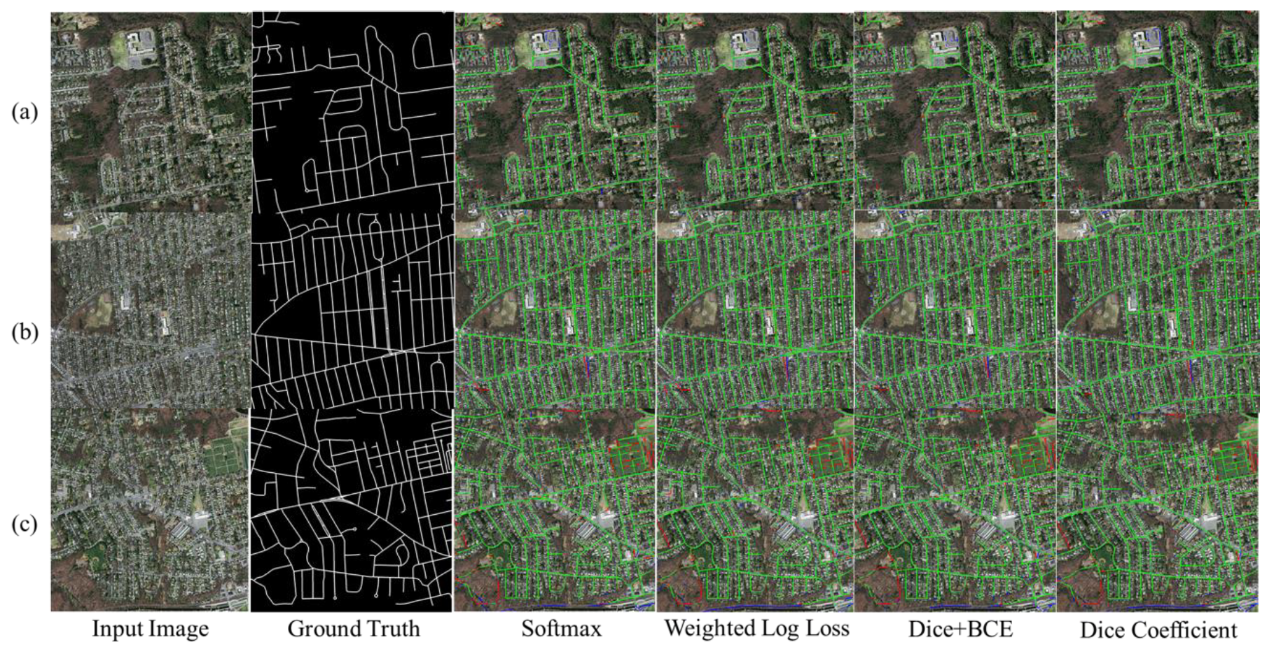
Visual comparison of four loss functions used with Nested SE-Deeplab on the testing set. True positive (TP) is marked as green, false positive (FP) as blue, and false negative (FN) as red. The three rows including (a), (b) and (c) in the figure represent visual effects of three examples in testing set, which have been tested by models with different loss functions. For each row in the figure, it contains an input image, a picture of ground truth and results of models with different loss functions including softmax cross entropy, weighted log loss, dice+bce and dice coefficient.
Figure 7.
Visual comparison of four loss functions used with Nested SE-Deeplab on the testing set. True positive (TP) is marked as green, false positive (FP) as blue, and false negative (FN) as red. The three rows including (a), (b) and (c) in the figure represent visual effects of three examples in testing set, which have been tested by models with different loss functions. For each row in the figure, it contains an input image, a picture of ground truth and results of models with different loss functions including softmax cross entropy, weighted log loss, dice+bce and dice coefficient.

Figure 8.
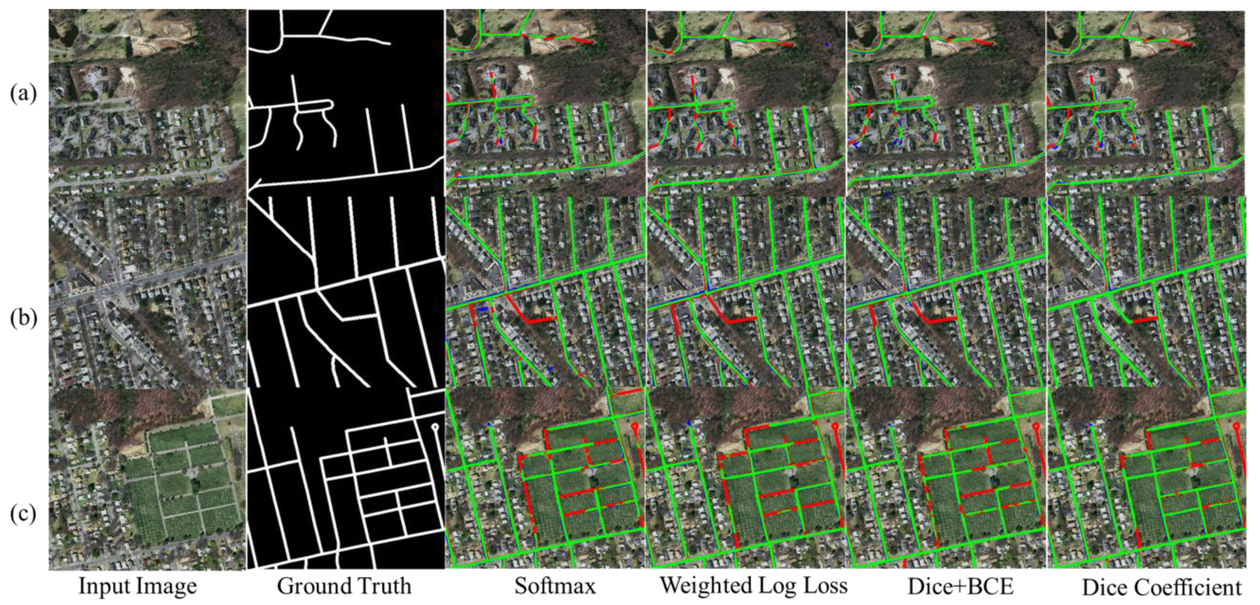
Magnification of the results in Figure 7. True positive (TP) is marked as green, false positive (FP) as blue, and false negative (FN) as red. Each subfigure in this figure is the magnification of the results shown in Figure 7.

Figure 9.
Progression of loss values (A) and training accuracy (B) for four loss functions used with Nested SE-Deeplab during training. The loss functions are softmax cross entropy (softmax), weighted log loss, dice coefficient (dice), and dice coefficient added with binary cross entropy (bce).
Figure 9.
Progression of loss values (A) and training accuracy (B) for four loss functions used with Nested SE-Deeplab during training. The loss functions are softmax cross entropy (softmax), weighted log loss, dice coefficient (dice), and dice coefficient added with binary cross entropy (bce).

Figure 10.
Visual comparison of three backbone networks used in Nested SE-Deeplab for the testing set. True positive (TP) is marked as green, false positive (FP) as blue, and false negative (FN) as red. The three rows including (a), (b) and (c) in the figure represent visual effects of three examples in testing set, which have been tested by different models. For each row in the figure, it contains an input image, a picture of ground truth and results of the proposed model combined with different backbone networks including ResNet, ResNext and SE Module.

Figure 11.
Magnification of the results in Figure 10. True positive (TP) is marked as green, false positive (FP) as blue, and false negative (FN) as red. Each subfigure in this figure is the magnification of the results shown in Figure 10.

Figure 12.
Visual comparison of Nested SE-Deeplab and other deep-learning models on the testing dataset. True positive (TP) is marked as green, false positive (FP) as blue, and false negative (FN) as red. The three rows including (a), (b) and (c) in the figure contains visual effects of three examples in testing set, which have been tested by different models. For each row in the figure, it contains an input image, a picture of ground truth and five results of road extraction models including Deeplab v3, SegNet, UNet, FC-DenseNet and Nested SE-Deeplab.

Figure 13.
Magnification of the results in Figure 12. True positive (TP) is marked as green, false positive (FP) as blue, and false negative (FN) as red. Each subfigure in this figure is the magnification of the results shown in Figure 12.


Table 1.
Detailed distribution of the dataset used in this study.
| Training Set | Validation Set | Test Set | |
|---|---|---|---|
| Images | 604 | 66 | 27 |
| Sub-Images | 96976 | 7654 | / |
Table 2.
Quantitative comparison of four loss functions for the testing dataset.
| Experiment | Methods | Correctness | F1-Score | IoU 1 |
|---|---|---|---|---|
| Figure 7a | Softmax | 0.8707 | 0.8821 | 0.7823 |
| WBCE | 0.8728 | 0.8806 | 0.7867 | |
| Dice+BCE | 0.8757 | 0.8823 | 0.7893 | |
| Dice | 0.8739 | 0.8836 | 0.7914 | |
| Figure 7b | Softmax | 0.9061 | 0.9101 | 0.8350 |
| WBCE | 0.9078 | 0.9098 | 0.8359 | |
| Dice+BCE | 0.9132 | 0.9136 | 0.8410 | |
| Dice | 0.9140 | 0.9167 | 0.8462 | |
| Figure 7c | Softmax | 0.8108 | 0.8355 | 0.7175 |
| WBCE | 0.8143 | 0.8364 | 0.7189 | |
| Dice+BCE | 0.8291 | 0.8441 | 0.7302 | |
| Dice | 0.8363 | 0.8497 | 0.7387 |
1 The full name of IoU is Intersection over Union.
Table 3.
Quantitative comparison of three backbone networks for the testing dataset.
| Experiment | Methods | Correctness | F1-Score | IoU 1 |
|---|---|---|---|---|
| Figure 10a | ResNet | 0.9100 | 0.9112 | 0.8385 |
| ResNext | 0.9088 | 0.9161 | 0.8455 | |
| SE-Net | 0.9140 | 0.9167 | 0.8462 | |
| Figure 10b | ResNet | 0.8152 | 0.8274 | 0.7056 |
| ResNext | 0.8395 | 0.8447 | 0.7312 | |
| SE-Net | 0.8380 | 0.8541 | 0.7454 | |
| Figure 10c | ResNet | 0.7941 | 0.8095 | 0.6800 |
| ResNext | 0.8120 | 0.8190 | 0.6935 | |
| SE-Net | 0.8270 | 0.8254 | 0.7027 |
1 The full name of IoU is Intersection over Union.
Table 4.
Quantitative comparison of Nested SE-Deeplab with other deep-learning models for the testing set.
Table 4.
Quantitative comparison of Nested SE-Deeplab with other deep-learning models for the testing set.
| Methods 1 | Overall Accuracy | Correctness | F1-Score | IoU 2 |
|---|---|---|---|---|
| Deeplab V3 | 0.862 | 0.694 | 0.734 | 0.5878 |
| SegNet | 0.873 | 0.695 | 0.724 | 0.6256 |
| U-Net | 0.923 | 0.793 | 0.821 | 0.6932 |
| ELU-SegNet-R | / | 0.847 | 0.812 | / |
| FC-DenseNet | 0.954 | 0.809 | 0.833 | 0.7189 |
| DCED | / | 0.839 | 0.829 | / |
| ASPP-UNet [60] | / | 0.849 | 0.832 | / |
| Our Methods | 0.967 | 0.858 | 0.857 | 0.7387 |
1 This table includes the results of this study and numerical results provided by other papers. 2 The full name of IoU is Intersection over Union.
Table 5.
Durations of two structures of Nested SE-Deeplab quantitatively compared.
| Prunning | No Prunning | |||
|---|---|---|---|---|
| Batches | Inference Time | Batches | Inference Time | |
| Nested SE-Deeplab | 10 | 1 m 42 s | 10 | 1 m 56 s |
© 2020 by the authors. Licensee MDPI, Basel, Switzerland. This article is an open access article distributed under the terms and conditions of the Creative Commons Attribution (CC BY) license (http://creativecommons.org/licenses/by/4.0/).
Share and Cite
MDPI and ACS Style
Lin, Y.; Xu, D.; Wang, N.; Shi, Z.; Chen, Q. Road Extraction from Very-High-Resolution Remote Sensing Images via a Nested SE-Deeplab Model. Remote Sens. 2020, 12, 2985. https://doi.org/10.3390/rs12182985
AMA Style
Lin Y, Xu D, Wang N, Shi Z, Chen Q. Road Extraction from Very-High-Resolution Remote Sensing Images via a Nested SE-Deeplab Model. Remote Sensing. 2020; 12(18):2985. https://doi.org/10.3390/rs12182985
Chicago/Turabian StyleLin, Yeneng, Dongyun Xu, Nan Wang, Zhou Shi, and Qiuxiao Chen. 2020. "Road Extraction from Very-High-Resolution Remote Sensing Images via a Nested SE-Deeplab Model" Remote Sensing 12, no. 18: 2985. https://doi.org/10.3390/rs12182985
Note that from the first issue of 2016, this journal uses article numbers instead of page numbers. See further details here.