Diurnal to Seasonal Variations in Ocean Chlorophyll and Ocean Currents in the North of Taiwan Observed by Geostationary Ocean Color Imager and Coastal Radar


Abstract
:
1. Introduction
1.1. Background
1.2. Objectives
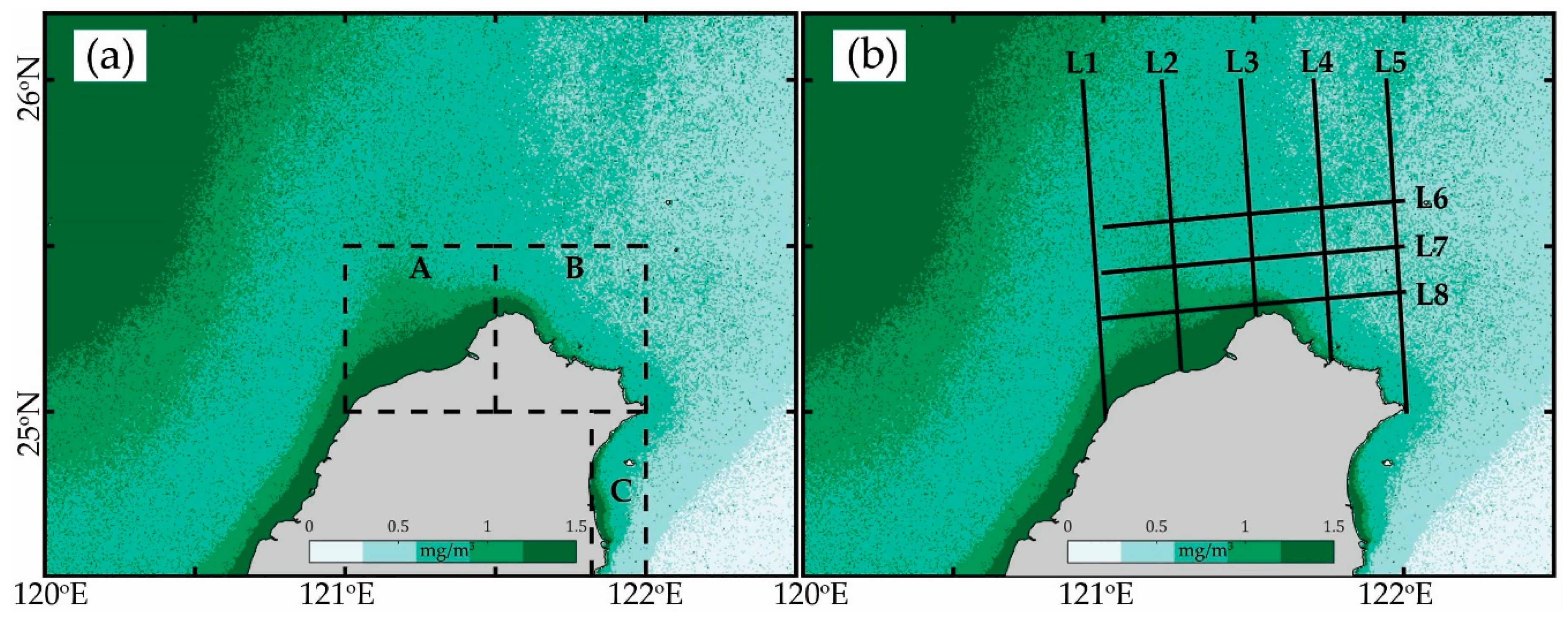
1.3. Study Area
2. Materials and Methods
2.1. Sea Surface Temperature and Chlorophyll Concentration
2.1.1. Geostationary Ocean Color Imager
2.1.2. Himawari-8
2.2. Ocean Currents
2.2.1. Buoy
2.2.2. Ship-Board ADCP
2.2.3. CODAR
2.3. Tide
2.4. Drifter
3. Results
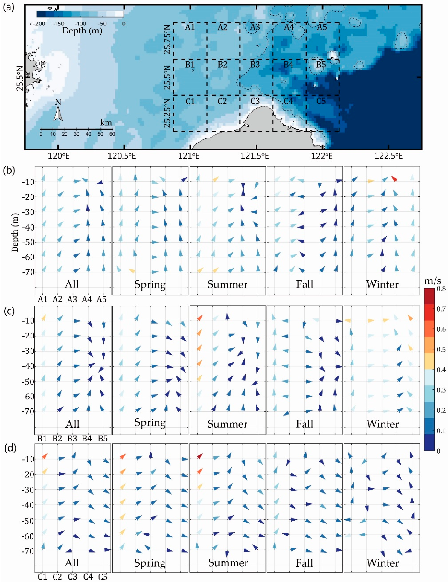
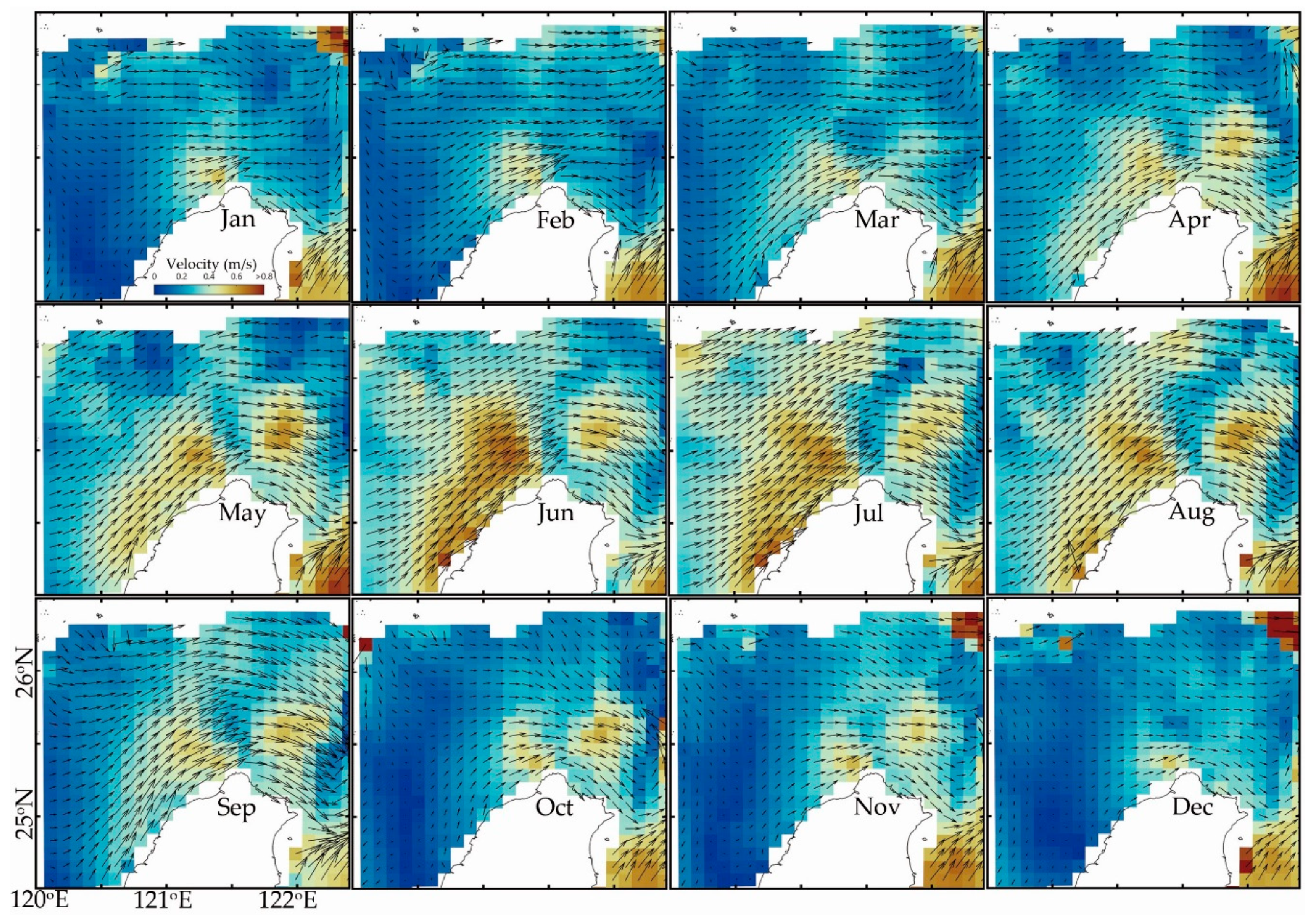
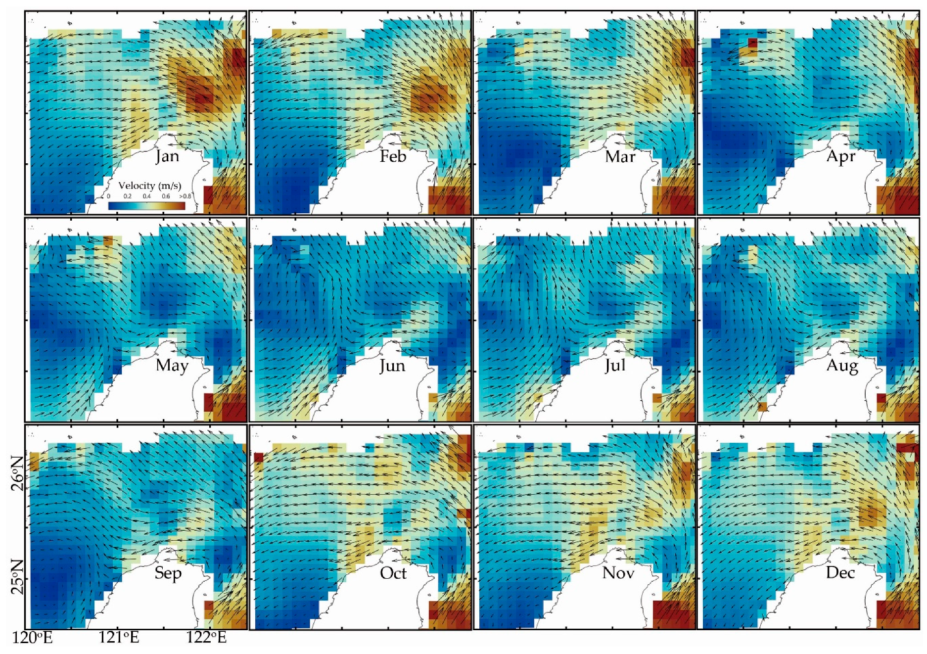
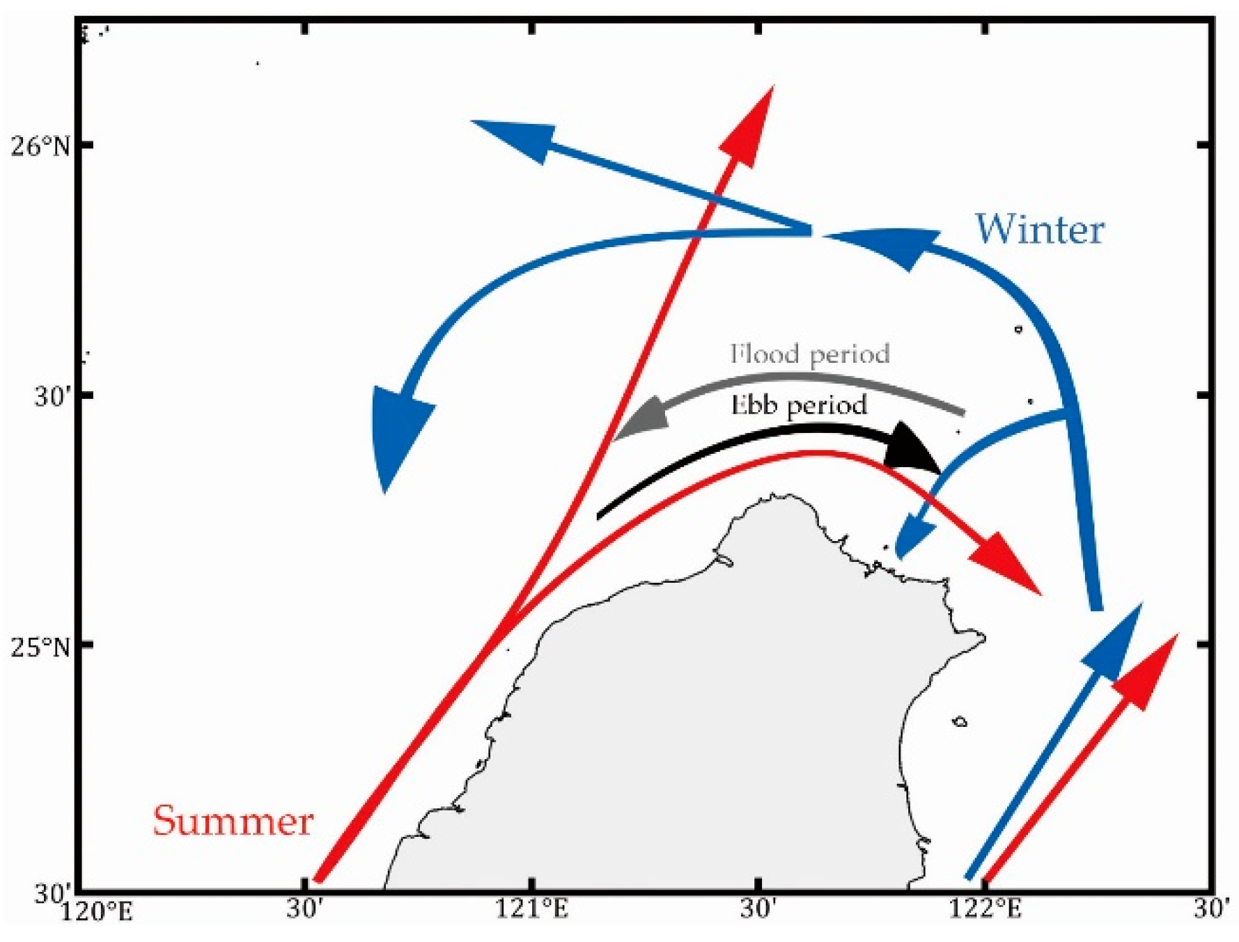
3.1. Characteristics of Ocean Current in Northern Taiwan
3.1.1. Historical Survey Observation
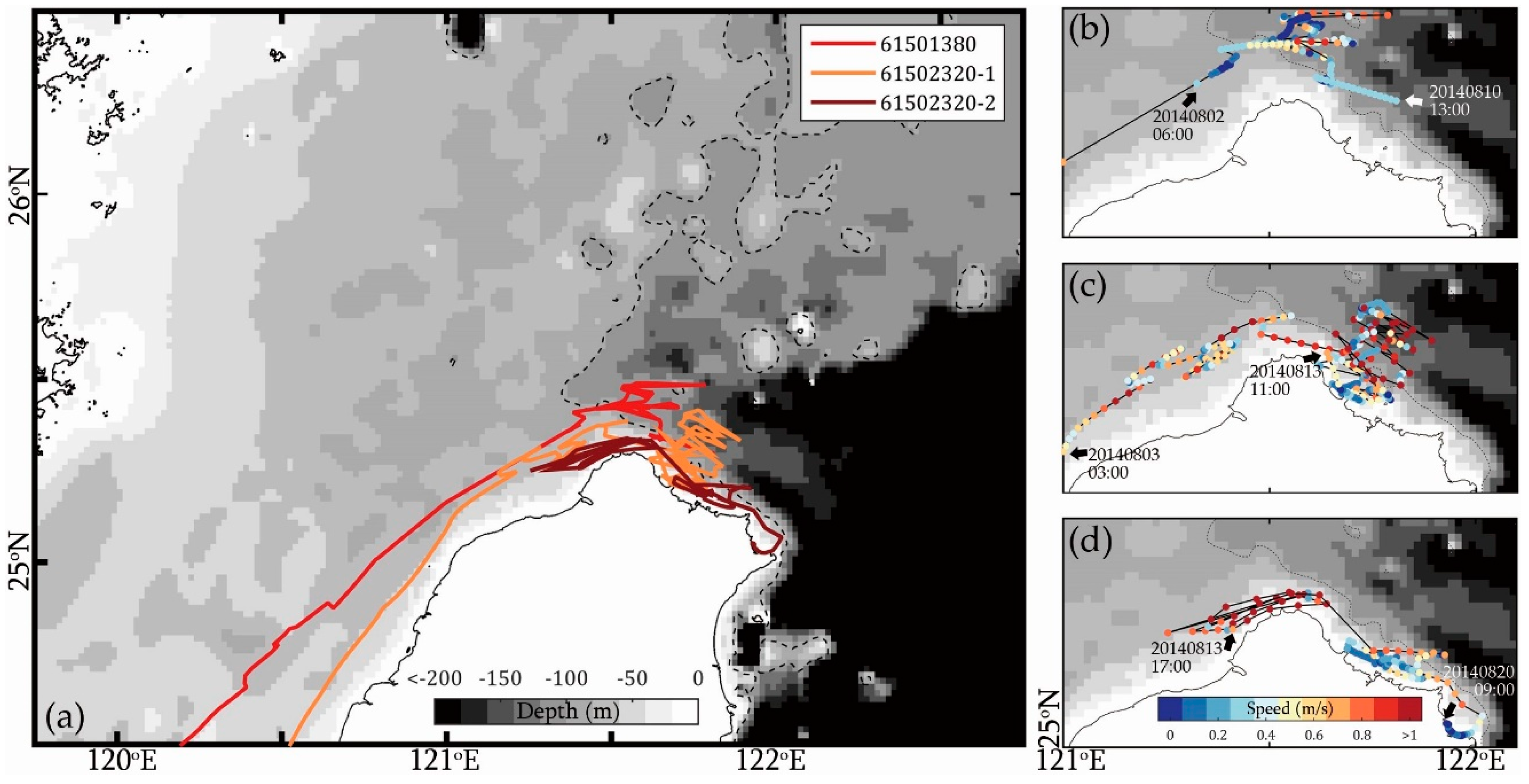
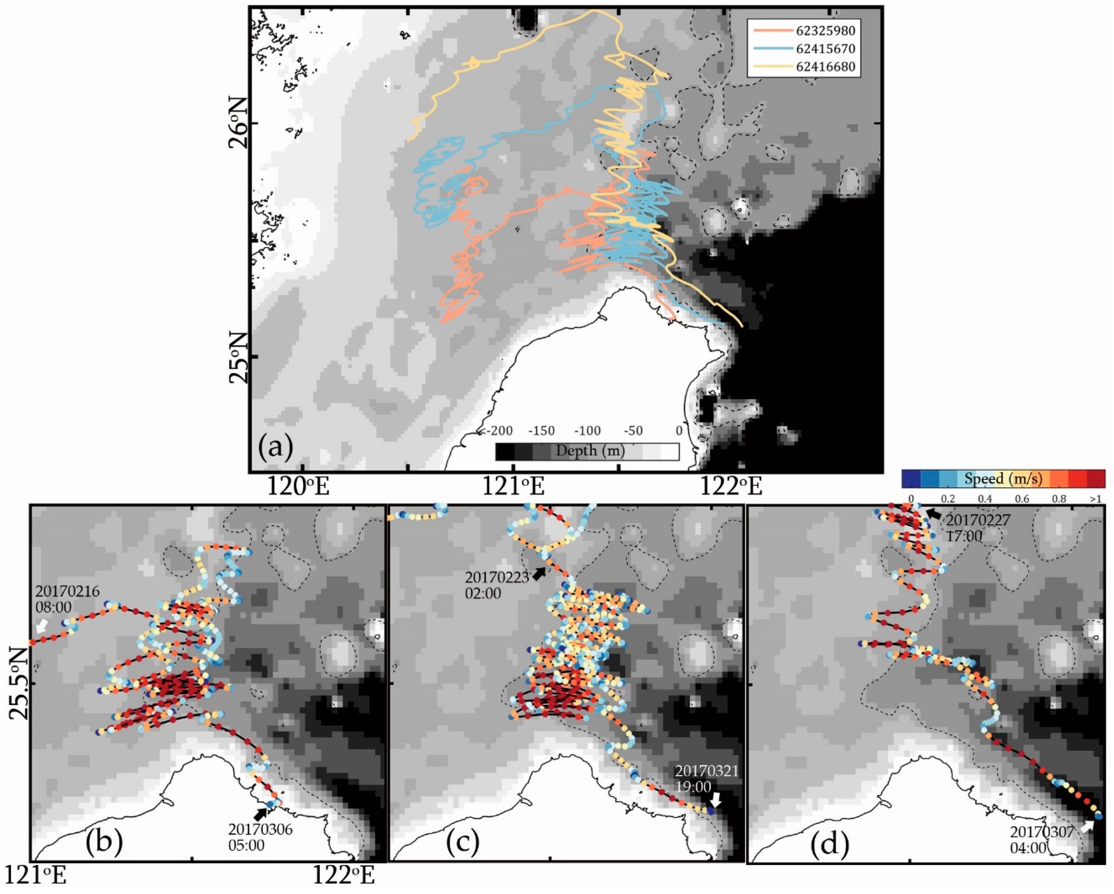
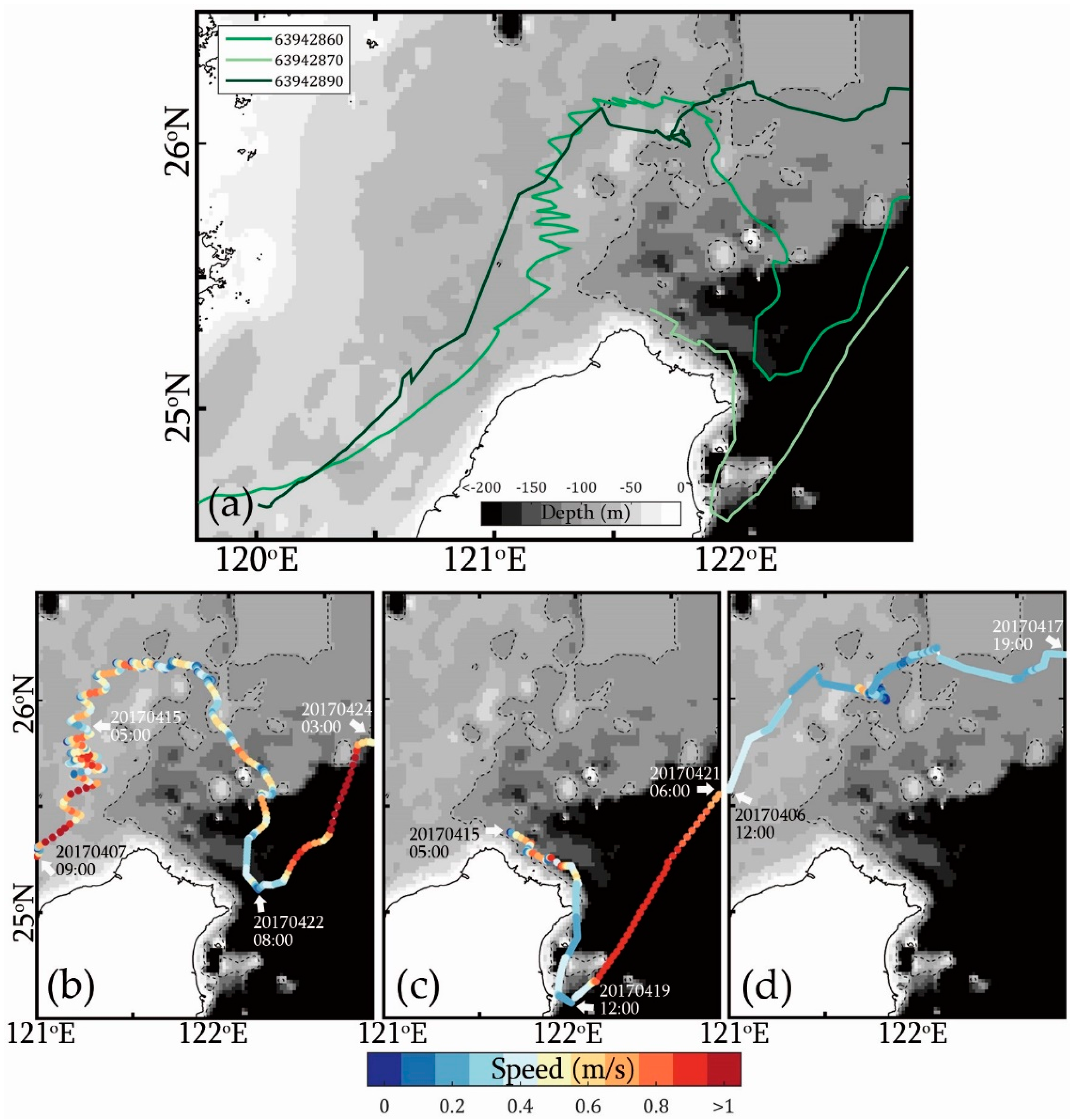
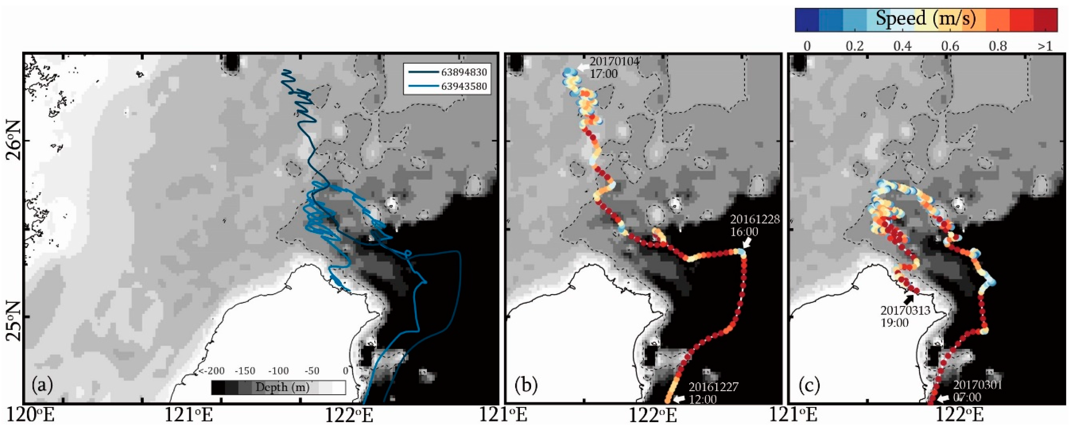
3.1.2. Drifter Experiments
3.2. Diurnal to Seasonal Changes in Chlorophyll Concentrations
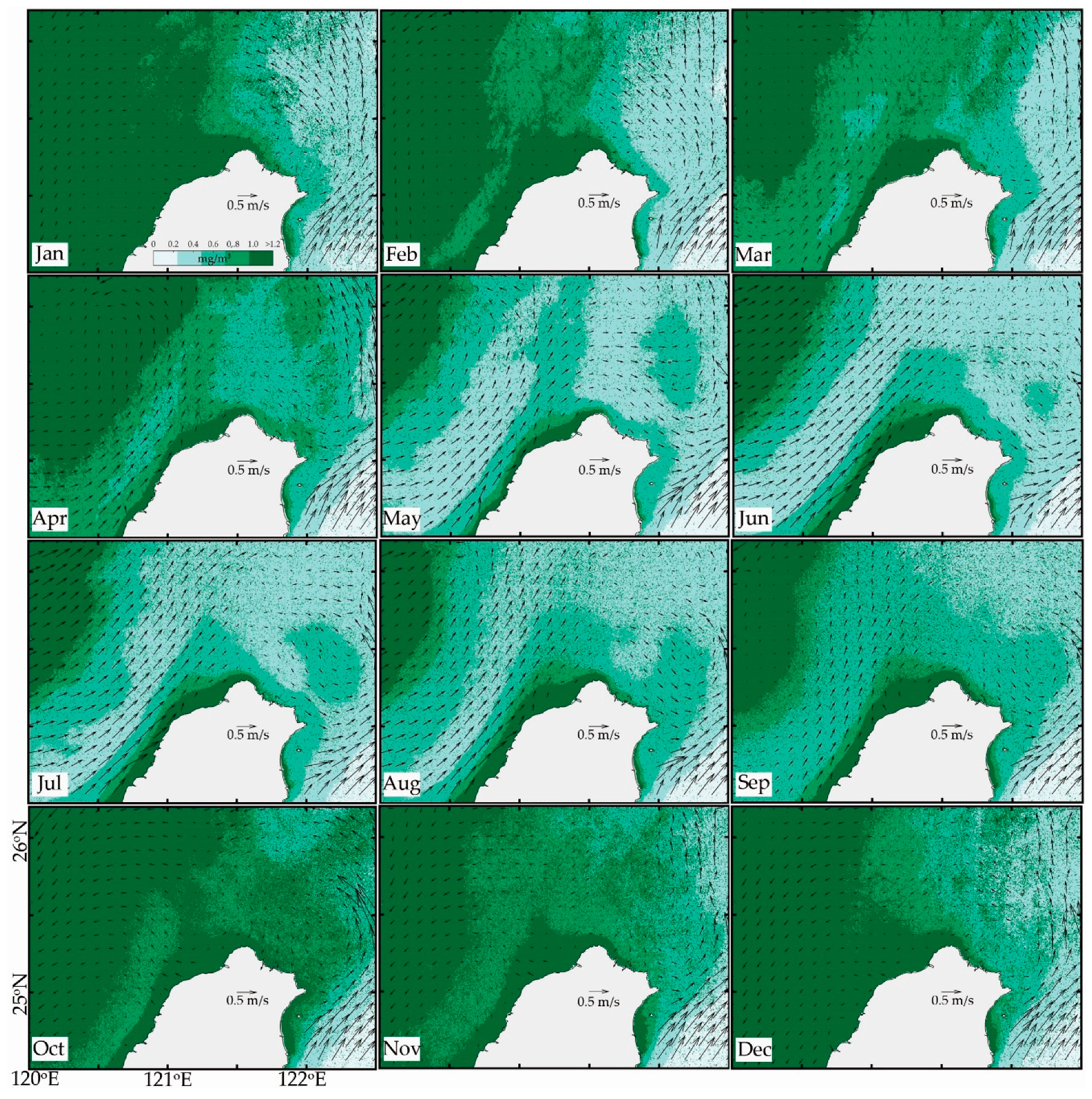
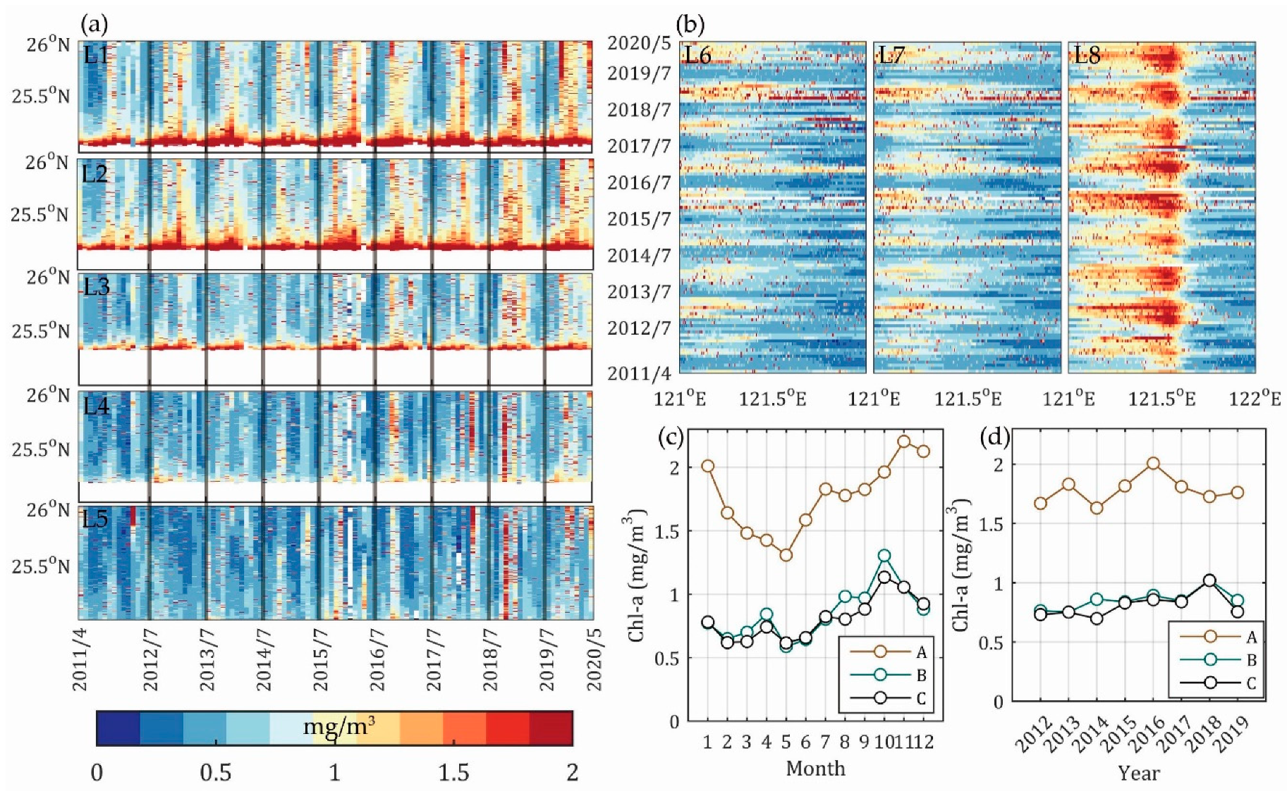
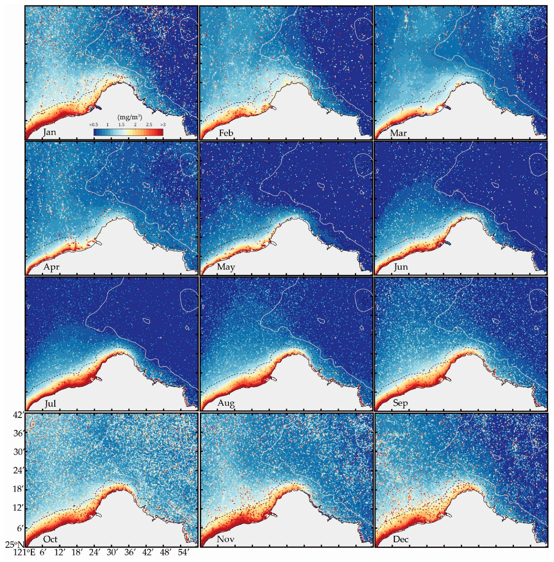
3.2.1. Monthly to Seasonal Variations
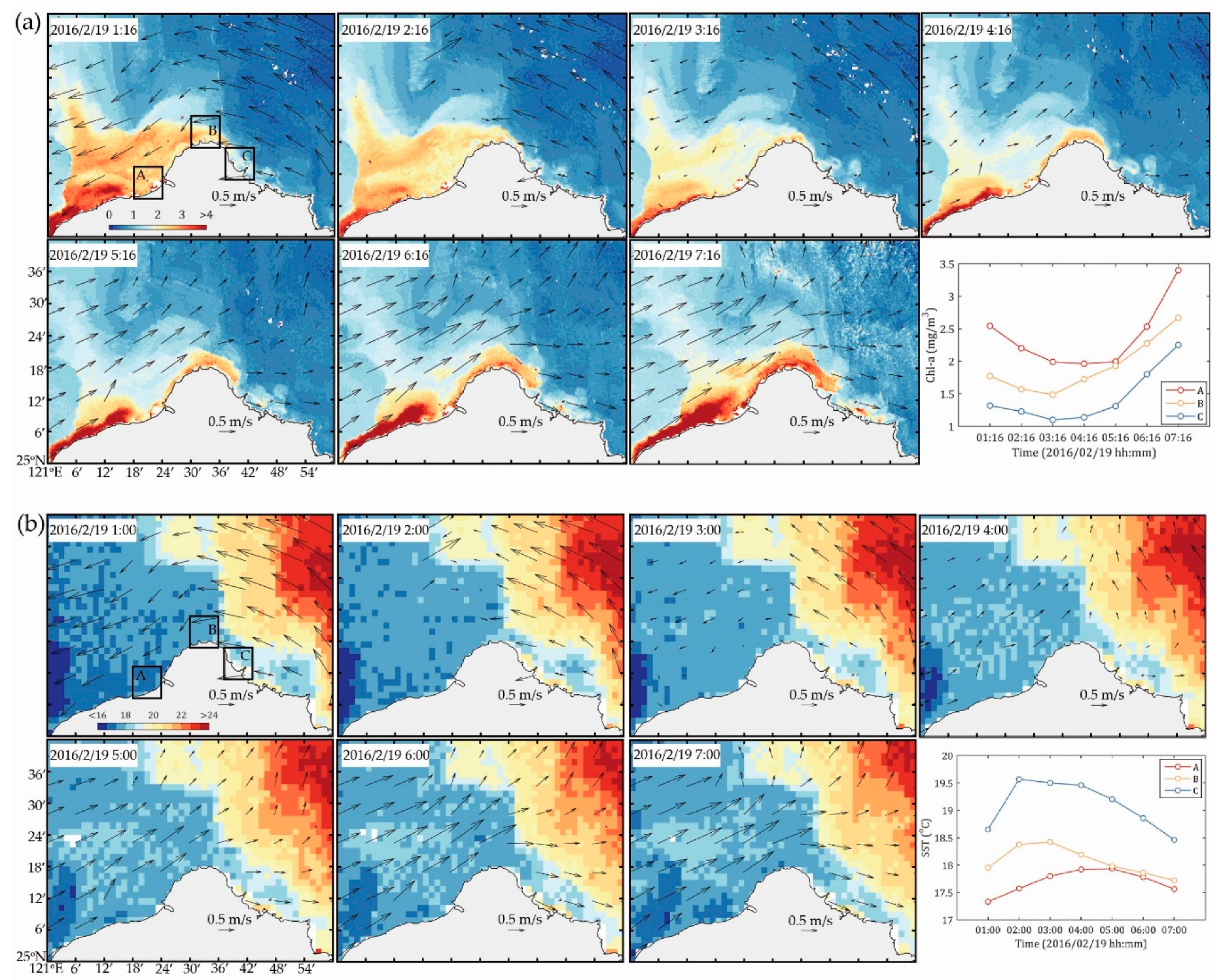
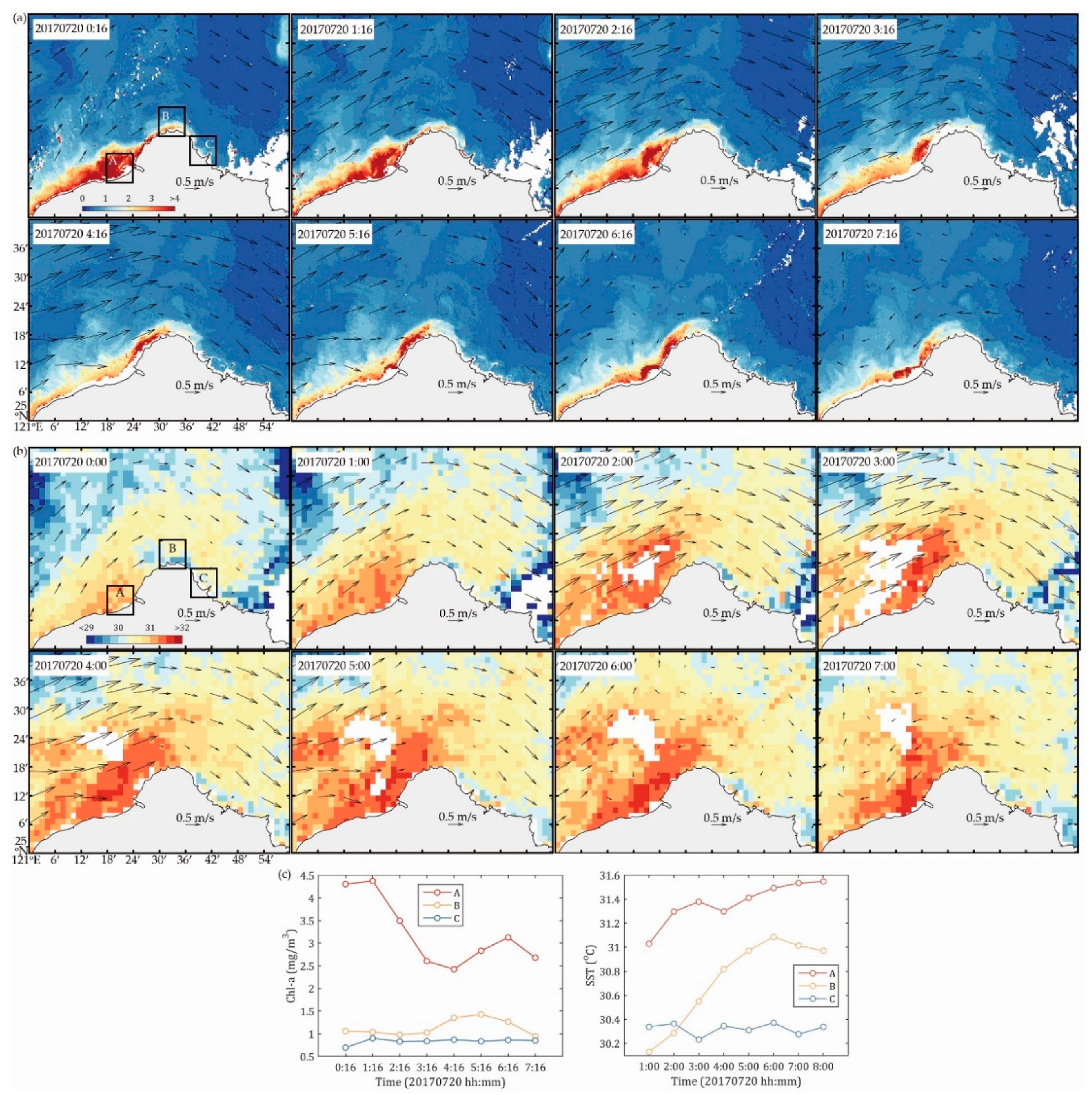
3.2.2. Diurnal Variation with Tidal Currents
4. Discussion
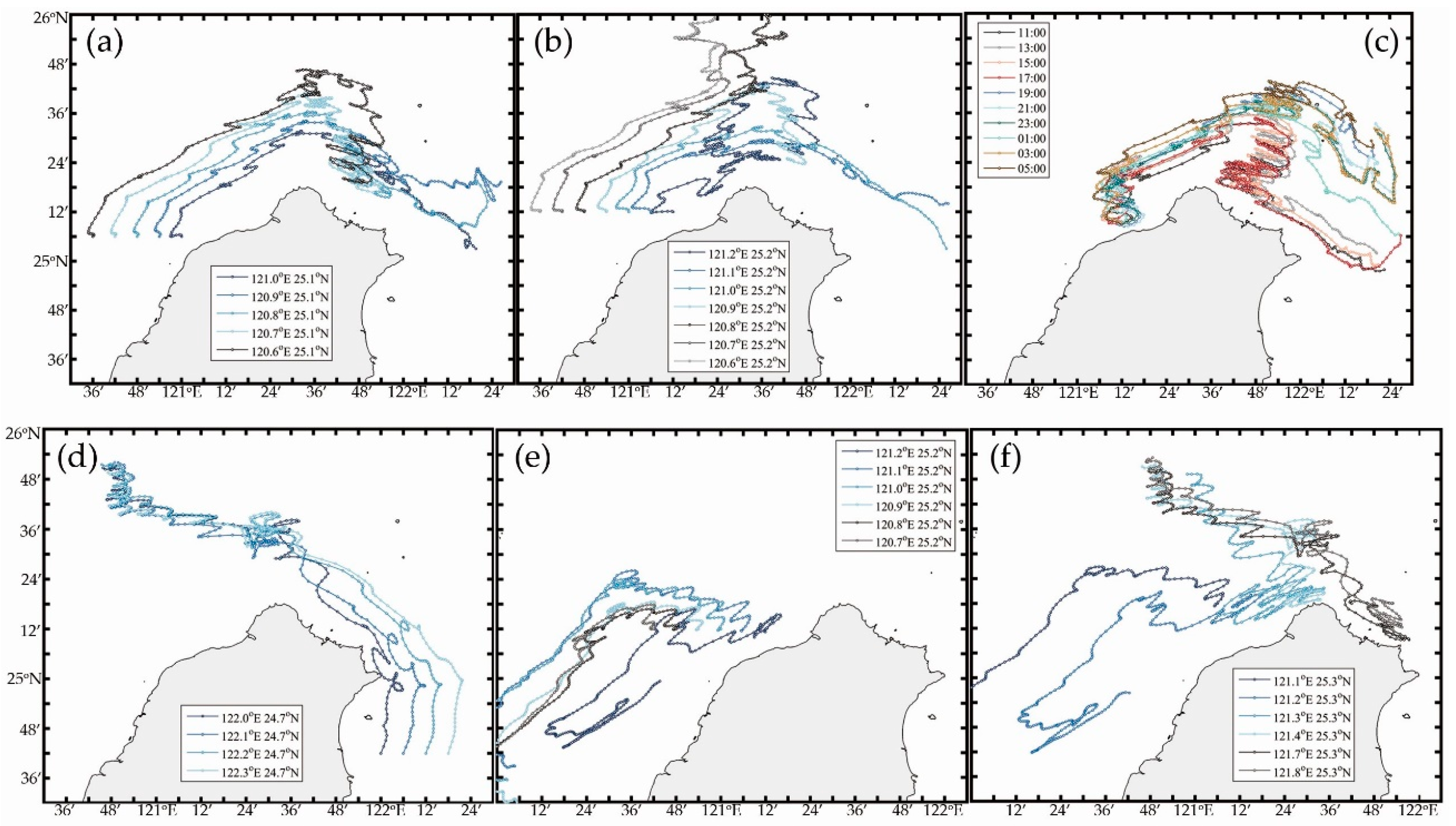
4.1. Current Trajectory Tracking Experiment
4.2. Compared with CODAR Flow Field with Buoy and Reanalysis Data
5. Conclusions
Author Contributions
Funding
Acknowledgments
Conflicts of Interest
Appendix A

| Spring (March to May) | ||||||||||||||
| D | S | D | S | D | S | D | S | D | S | |||||
| A1 | N | 0.33 | A2 | N | 0.17 | A3 | ESE | 0.29 | A4 | NW | 0.29 | A5 | NE | 0.04 |
| B1 | NNE | 0.35 | B2 | NNE | 0.18 | B3 | ESE | 0.12 | B4 | SE | 0.20 | B5 | SE | 0.18 |
| C1 | NE | 0.63 | C2 | ENE | 0.14 | C3 | N | 0.05 | C4 | SE | 0.09 | C5 | E | 0.15 |
| Summer (Jun to August) | ||||||||||||||
| D | S | D | S | D | S | D | S | D | S | |||||
| A1 | NNE | 0.29 | A2 | NE | 0.45 | A3 | ENE | 0.31 | A4 | S | 0.08 | A5 | SSW | 0.18 |
| B1 | NE | 0.63 | B2 | NE | 0.33 | B3 | N | 0.03 | B4 | SE | 0.08 | B5 | S | 0.21 |
| C1 | NE | 0.80 | C2 | ENE | 0.21 | C3 | NNE | 0.15 | C4 | SSE | 0.15 | C5 | SE | 0.22 |
| Fall (September to November) | ||||||||||||||
| D | S | D | S | D | S | D | S | D | S | |||||
| A1 | NE | 0.38 | A2 | NE | 0.25 | A3 | WNW | 0.31 | A4 | S | 0.13 | A5 | ENE | 0.07 |
| B1 | NNW | 0.26 | B2 | W | 0.18 | B3 | SSW | 0.15 | B4 | WNW | 0.33 | B5 | E | 0.05 |
| C1 | NNE | 0.26 | C2 | SSW | 0.02 | C3 | N | 0.09 | C4 | SE | 0.07 | C5 | SE | 0.15 |
| Winter (December to February) | ||||||||||||||
| D | S | D | S | D | S | D | S | D | S | |||||
| A1 | NE | 0.12 | A2 | E | 0.44 | A3 | NE | 0.17 | A4 | NW | 0.70 | A5 | N | 0.34 |
| B1 | W | 0.46 | B2 | E | 0.45 | B3 | ENE | 0.42 | B4 | NNW | 0.38 | B5 | NW | 0.50 |
| C1 | NNW | 0.14 | C2 | SW | 0.19 | C3 | NE | 0.14 | C4 | SSE | 0.07 | C5 | NNW | 0.07 |
| Spring (March to May) | ||||||||||||||
| D | S | D | S | D | S | D | S | D | S | |||||
| A1 | N | 0.17 | A2 | NNE | 0.13 | A3 | NE | 0.04 | A4 | ENE | 0.07 | A5 | NE | 0.09 |
| B1 | NNE | 0.20 | B2 | NE | 0.16 | B3 | ENE | 0.05 | B4 | ESE | 0.09 | B5 | E | 0.09 |
| C1 | NNE | 0.20 | C2 | NNE | 0.09 | C3 | NE | 0.06 | C4 | SSE | 0.08 | C5 | ESE | 0.11 |
| Summer (Jun to September) | ||||||||||||||
| D | S | D | S | D | S | D | S | D | S | |||||
| A1 | NNE | 0.29 | A2 | NE | 0.22 | A3 | NE | 0.09 | A4 | E | 0.08 | A5 | ESE | 0.12 |
| B1 | NE | 0.32 | B2 | NE | 0.23 | B3 | ENE | 0.07 | B4 | SE | 0.08 | B5 | SE | 0.11 |
| C1 | NE | 0.27 | C2 | NE | 0.12 | C3 | NE | 0.04 | C4 | S | 0.06 | C5 | SE | 0.14 |
| Fall (October and November) | ||||||||||||||
| D | S | D | S | D | S | D | S | D | S | |||||
| A1 | WNW | 0.09 | A2 | WSW | 0.04 | A3 | SSW | 0.06 | A4 | NNE | 0.02 | A5 | NE | 0.04 |
| B1 | WNW | 0.07 | B2 | WSW | 0.01 | B3 | SSE | 0.04 | B4 | SE | 0.06 | B5 | ESE | 0.05 |
| C1 | NW | 0.09 | C2 | W | 0.06 | C3 | NNE | 0.01 | C4 | SSW | 0.11 | C5 | SE | 0.09 |
| Winter (December to February) | ||||||||||||||
| D | S | D | S | D | S | D | S | D | S | |||||
| A1 | W | 0.06 | A2 | W | 0.05 | A3 | W | 0.05 | A4 | WNW | 0.16 | A5 | NW | 0.21 |
| B1 | WNW | 0.04 | B2 | WSW | 0.02 | B3 | W | 0.01 | B4 | WNW | 0.12 | B5 | NW | 0.17 |
| C1 | WNW | 0.05 | C2 | WSW | 0.04 | C3 | NNW | 0.03 | C4 | SW | 0.09 | C5 | WNW | 0.05 |
| Spring (March to May) | ||||||||||||||
| D | S | D | S | D | S | D | S | D | S | |||||
| A1 | ENE | 0.31 | A2 | ENE | 0.32 | A3 | E | 0.26 | A4 | E | 0.37 | A5 | E | 0.38 |
| B1 | ENE | 0.39 | B2 | ENE | 0.47 | B3 | E | 0.31 | B4 | ESE | 0.43 | B5 | ESE | 0.40 |
| C1 | NE | 0.43 | C2 | ENE | 0.42 | C3 | ENE | 0.40 | C4 | ESE | 0.38 | C5 | ESE | 0.36 |
| Summer (Jun to September) | ||||||||||||||
| D | S | D | S | D | S | D | S | D | S | |||||
| A1 | ENE | 0.48 | A2 | ENE | 0.43 | A3 | ENE | 0.28 | A4 | ESE | 0.38 | A5 | ESE | 0.47 |
| B1 | NE | 0.55 | B2 | ENE | 0.58 | B3 | ENE | 0.31 | B4 | ESE | 0.44 | B5 | ESE | 0.47 |
| C1 | NE | 0.51 | C2 | ENE | 0.48 | C3 | ENE | 0.37 | C4 | ESE | 0.35 | C5 | ESE | 0.39 |
| Fall (Oct and November) | ||||||||||||||
| D | S | D | S | D | S | D | S | D | S | |||||
| A1 | E | 0.19 | A2 | E | 0.31 | A3 | ESE | 0.30 | A4 | E | 0.34 | A5 | ESE | 0.40 |
| B1 | ENE | 0.24 | B2 | E | 0.43 | B3 | E | 0.34 | B4 | ESE | 0.44 | B5 | ESE | 0.44 |
| C1 | ENE | 0.25 | C2 | ENE | 0.36 | C3 | ENE | 0.39 | C4 | ESE | 0.35 | C5 | SE | 0.36 |
| Winter (December to February) | ||||||||||||||
| D | S | D | S | D | S | D | S | D | S | |||||
| A1 | E | 0.21 | A2 | E | 0.27 | A3 | E | 0.25 | A4 | E | 0.23 | A5 | E | 0.20 |
| B1 | ENE | 0.25 | B2 | E | 0.38 | B3 | E | 0.31 | B4 | E | 0.25 | B5 | E | 0.21 |
| C1 | ENE | 0.26 | C2 | ENE | 0.35 | C3 | ENE | 0.35 | C4 | ESE | 0.30 | C5 | ESE | 0.24 |
| Spring (March to May) | ||||||||||||||
| D | S | D | S | D | S | D | S | D | S | |||||
| A1 | WNW | 0.30 | A2 | WNW | 0.26 | A3 | WNW | 0.24 | A4 | WNW | 0.32 | A5 | NW | 0.38 |
| B1 | WNW | 0.25 | B2 | W | 0.29 | B3 | W | 0.26 | B4 | WNW | 0.33 | B5 | WNW | 0.31 |
| C1 | WNW | 0.20 | C2 | W | 0.35 | C3 | WSW | 0.36 | C4 | WSW | 0.32 | C5 | WNW | 0.20 |
| Summer (Jun to September) | ||||||||||||||
| D | S | D | S | D | S | D | S | D | S | |||||
| A1 | NNW | 0.27 | A2 | NW | 0.21 | A3 | WNW | 0.18 | A4 | WNW | 0.27 | A5 | WNW | 0.29 |
| B1 | NNW | 0.22 | B2 | WNW | 0.26 | B3 | W | 0.21 | B4 | W | 0.36 | B5 | WNW | 0.33 |
| C1 | NW | 0.17 | C2 | WSW | 0.32 | C3 | WSW | 0.34 | C4 | W | 0.36 | C5 | W | 0.17 |
| Fall (October and November) | ||||||||||||||
| D | S | D | S | D | S | D | S | D | S | |||||
| A1 | W | 0.40 | A2 | W | 0.44 | A3 | W | 0.40 | A4 | WNW | 0.38 | A5 | WNW | 0.41 |
| B1 | W | 0.37 | B2 | W | 0.51 | B3 | W | 0.36 | B4 | W | 0.41 | B5 | WNW | 0.39 |
| C1 | W | 0.40 | C2 | WSW | 0.54 | C3 | WSW | 0.43 | C4 | W | 0.39 | C5 | WNW | 0.23 |
| Winter (December to February) | ||||||||||||||
| D | S | D | S | D | S | D | S | D | S | |||||
| A1 | W | 0.36 | A2 | W | 0.41 | A3 | W | 0.40 | A4 | WNW | 0.59 | A5 | WNW | 0.63 |
| B1 | W | 0.36 | B2 | WSW | 0.49 | B3 | W | 0.36 | B4 | WNW | 0.52 | B5 | WNW | 0.57 |
| C1 | WSW | 0.38 | C2 | WSW | 0.49 | C3 | WSW | 0.42 | C4 | W | 0.43 | C5 | WNW | 0.38 |
References
- Jan, S.; Wang, J.; Chern, C.S.; Chao, S.Y. Seasonal variation of the circulation in the Taiwan Strait. J. Mar. Syst. 2002, 35, 249–268. [Google Scholar] [CrossRef]
- Jan, S.; Sheu, D.D.; Kuo, H.M. Water mass and throughflow transport variability in the Taiwan Strait. J. Geophys. Res. Oceans 2006, 111, C12012. [Google Scholar] [CrossRef]
- Tseng, H.C.; You, W.L.; Huang, W.; Chung, C.C.; Tsai, A.Y.; Chen, T.Y.; Lan, K.W.; Gong, G.C. Seasonal variations of marine environment and primary production in the Taiwan Strait. Front. Mar. Sci. 2020, 7, 38. [Google Scholar] [CrossRef]
- Hsieh, C.H.; Chen, C.S.; Chiu, T.S. Composition and abundance of copepods and ichthyoplankton in Taiwan Strait (western North Pacific) are influenced by seasonal monsoons. Mar. Freshw. Res 2005, 56, 153–161. [Google Scholar] [CrossRef]
- Hwang, J.S.; Souissi, S.; Tseng, L.C.; Seuront, L.; Schmitt, F.G.; Fang, L.S.; Peng, S.H.; Wu, C.H.; Hsiao, S.H.; Twan, W.H.; et al. A 5-year study of the influence of the northeast and southwest monsoons on copepod assemblages in the boundary coastal waters between the East China Sea and the Taiwan Strait. J. Plankton Res. 2006, 28, 943–958. [Google Scholar] [CrossRef] [Green Version]
- Chen, H.Y.; Chen, Y.L.L. Quantity and quality of summer surface net zooplankton in the Kuroshio current-induced upwelling northeast of Taiwan. Terr. Atmos. Ocean. Sci. 1992, 3, 321–334. [Google Scholar] [CrossRef]
- Su, W.C.; Lo, W.T.; Liu, D.C.; Wu, L.J.; Hsieh, H.Y. Larval fish assemblages in the Kuroshio waters east of Taiwan during two distinct monsoon seasons. Bull. Mar. Sci. 2011, 87, 13–29. [Google Scholar] [CrossRef]
- Naimullah, M.; Lan, K.W.; Liao, C.H.; Hsiao, P.Y.; Liang, Y.R.; Chiu, T.C. Association of environmental factors in the taiwan strait with distributions and habitat characteristics of three swimming crabs. Remote Sens. 2020, 12, 2231. [Google Scholar] [CrossRef]
- Choi, J.; Park, Y.G.; Kim, W.; Kim, Y.H. Characterization of submesoscale turbulence in the east/japan sea using geostationary ocean color satellite images. Geophys. Res. Lett. 2019, 46, 8214–8223. [Google Scholar] [CrossRef]
- Higa, H.; Sugahara, S.; Salem, S.I.; Nakamura, Y.; Suzuki, T. An estimation method for blue tide distribution in Tokyo Bay based on sulfur concentrations using Geostationary Ocean Color Imager (GOCI). Estuar. Coast. Shelf Sci. 2020, 235, 106615. [Google Scholar] [CrossRef]
- Park, J.E.; Park, K.A.; Kang, C.K.; Park, Y.J. Short-term response of chlorophyll-a concentration to change in sea surface wind field over mesoscale eddy. Estuar. Coasts 2020, 43, 646–660. [Google Scholar] [CrossRef]
- Jan, S.; Chen, C.C.; Tsai, Y.L.; Yang, Y.J.; Wang, J.; Chern, C.S.; Gawarkiewicz, G.; Lien, R.C.; Centurioni, L.; Kuo, J.Y. Mean structure and variability of the cold dome northeast of Taiwan. Oceanography 2011, 24, 100–109. [Google Scholar] [CrossRef] [Green Version]
- Hsu, P.C.; Zheng, Q.; Lu, C.Y.; Cheng, K.H.; Lee, H.J.; Ho, C.R. Interaction of coastal countercurrent in I-Lan Bay with the Kuroshio northeast of Taiwan. Cont. Shelf Res. 2018, 171, 30–41. [Google Scholar] [CrossRef]
- Yin, Y.; Liu, Z.; Hu, P.; Hou, Y.; Lu, J.; He, Y. Impact of mesoscale eddies on the southwestward countercurrent northeast of Taiwan revealed by ADCP mooring observations. Cont. Shelf Res. 2020, 195, 104063. [Google Scholar] [CrossRef]
- He, Y.; Hu, P.; Yin, Y.; Liu, Z.; Liu, Y.; Hou, Y.; Zhang, Y. Vertical migration of the along-slope counter-flow and its relation with the Kuroshio intrusion off northeastern Taiwan. Remote Sens. 2019, 11, 2624. [Google Scholar] [CrossRef] [Green Version]
- Shen, Y.T.; Lai, J.W.; Leu, L.G.; Lu, Y.C.; Chen, J.M.; Shao, H.J.; Chen, H.W.; Chang, K.T.; Terng, C.T.; Chang, Y.C.; et al. Applications of ocean currents data from high-frequency radars and current profilers to search and rescue missions around Taiwan. J. Oper. Oceanogr. 2019, 12 (Suppl. 2), S126–S136. [Google Scholar] [CrossRef] [Green Version]
- Hsu, P.C.; Lee, H.J.; Zheng, Q.; Lai, J.W.; Su, F.C.; Ho, C.R. Tide-induced periodic sea surface temperature drops in the coral reef area of Nanwan Bay, southern Taiwan. J. Geophys. Res. Oceans 2020, 125, e2019JC015226. [Google Scholar] [CrossRef]
- NASA Goddard Space Flight Center, Ocean Ecology Laboratory, Ocean Biology Processing Group. Geostationary Ocean Color Imager (GOCI) Ocean Color Data; 2014 Reprocessing; NASA OB.DAAC: Greenbelt, MD, USA, 2014. Available online: https://oceancolor.gsfc.nasa.gov/data/10.5067/COMS/GOCI/L2/OC/2014 (accessed on 23 June 2020).
- Hsu, P.C.; Ho, C.Y.; Lee, H.J.; Lu, C.Y.; Ho, C.R. Temporal variation and spatial structure of the Kuroshio-induced submesoscale island vortices observed from GCOM-C and Himawari-8 data. Remote Sens. 2020, 12, 883. [Google Scholar] [CrossRef] [Green Version]
- Elipot, S.; Lumpkin, R.; Perez, R.C.; Lilly, J.M.; Early, J.J.; Sykulski, A.M. A global surface drifter data set at hourly resolution. J. Geophys. Res. Oceans 2016, 121, 2937–2966. [Google Scholar] [CrossRef]
- Chen, C.T.A. Distributions of nutrients in the East China Sea and the South China Sea connection. J. Oceanogr. 2008, 64, 737–751. [Google Scholar] [CrossRef]


© 2020 by the authors. Licensee MDPI, Basel, Switzerland. This article is an open access article distributed under the terms and conditions of the Creative Commons Attribution (CC BY) license (http://creativecommons.org/licenses/by/4.0/).
Share and Cite
Hsu, P.-C.; Lu, C.-Y.; Hsu, T.-W.; Ho, C.-R. Diurnal to Seasonal Variations in Ocean Chlorophyll and Ocean Currents in the North of Taiwan Observed by Geostationary Ocean Color Imager and Coastal Radar. Remote Sens. 2020, 12, 2853. https://doi.org/10.3390/rs12172853
Hsu P-C, Lu C-Y, Hsu T-W, Ho C-R. Diurnal to Seasonal Variations in Ocean Chlorophyll and Ocean Currents in the North of Taiwan Observed by Geostationary Ocean Color Imager and Coastal Radar. Remote Sensing. 2020; 12(17):2853. https://doi.org/10.3390/rs12172853
Chicago/Turabian StyleHsu, Po-Chun, Ching-Yuan Lu, Tai-Wen Hsu, and Chung-Ru Ho. 2020. "Diurnal to Seasonal Variations in Ocean Chlorophyll and Ocean Currents in the North of Taiwan Observed by Geostationary Ocean Color Imager and Coastal Radar" Remote Sensing 12, no. 17: 2853. https://doi.org/10.3390/rs12172853