A New Approach for Soil Moisture Downscaling in the Presence of Seasonal Difference


School of Geography and Tourism, Shaanxi Normal University, Xi’an 710119, China
*
Author to whom correspondence should be addressed.
Remote Sens. 2020, 12(17), 2818; https://doi.org/10.3390/rs12172818
Submission received: 8 July 2020
/
Revised: 25 August 2020
/
Accepted: 26 August 2020
/
Published: 31 August 2020
(This article belongs to the Section Remote Sensing in Agriculture and Vegetation)
Abstract
:The variation of soil moisture (SM) is a complex and synthetic process, which is impacted by numerous factors. The effects of these factors on soil moisture are dynamic. As a result, the relationship between soil moisture and explanatory variables varies with time and season. This kind of change should be considered in obtaining fine spatial resolution soil moisture products. We chose a study area with four distinct seasons in the temperate monsoon region. In this research, we established seasonal downscaling models to avoid the influence of seasonal differences. Precipitation, land surface temperature, evapotranspiration, vegetation index, land cover, elevation, slope, aspect and soil texture were taken as explanatory variables to produce fine spatial resolution SM. SM products derived from Advanced Microwave Scanning Radiometer–Earth Observing System (AMSR-E) and Advanced Microwave Scanning Radiometer 2 (AMSR2) were downscaled with the help of machine learning algorithms. We compared three machine learning algorithms of random forest (RF), support vector machine (SVM), and K-nearest neighbors (KNN) to determine the most suitable algorithm for this study. The results show that season-based downscaling is even better than continuous time series. In the analysis of seasonal differences, precipitation plays a dominant role, but its contribution rate is different in each season. Moreover, the influence of vegetation is more prominent in winter, while the influence of terrain is more important in the other three seasons. It could be noted that the accuracy of the RF model is the best among three machine learning algorithms, and the RF-downscaled products have superior matching performance to both AMSR (AMSR-E and AMSR2) SM products and in-situ measurements. The analysis indicates considering seasonal difference and the application of machine learning has high potential for spatial downscaling in remote sensing applications.
1. Introduction
Soil moisture (SM) is an essential climate variable influencing land-atmosphere interactions, an essential hydrologic variable impacting rainfall-runoff processes, an essential ecological variable regulating net ecosystem exchange, and an essential agricultural variable [1,2,3,4]. Many ground stations have been set up to monitor soil moisture, but due to the limitation of number and uneven distributions, the in-situ measurements are insufficient for representing the soil moisture with large range [5]. With the development of remote sensing technology, we can get spatio-temporally continuous datasets on a large scale. Passive microwave satellites have been widely used to estimate SM over the past decades without the limitation of weather. However, passive microwave satellites have a coarse spatial resolution [6], which limits their soil moisture products in applications such as crop management, drought monitoring, fine-scale water budget assessment, and ecological modelling [7]. Therefore, it is necessary to improve the spatial resolution for the effective application of passive microwave derived SM products [8].
There are various passive microwave satellites that provide SM products, such as the Advanced Microwave Scanning Radiometer for Earth Observing System (AMSR-E) [9], the Advanced Microwave Scanning Radiometer 2 (AMSR2) [10], the Soil Moisture and Ocean Salinity (SMOS) [11], the Fengyun-3B (FY-3B) [12], the Soil Moisture Active Passive (SMAP) [13]. Among them, the AMSR series satellites including AMSR-E and AMSR2 are a satellite series with earlier launch time, longer duration, and still in operation. Moreover, AMSR SM products are more conducive to long-term research in drought detection and agricultural cultivation. Therefore, here we focus on SM retrieved from the AMSR instrument.
There are different methods of soil moisture downscaling, such as multivariate statistical regression methods, physical model-based methods, weight decomposition methods, data assimilation, and spatial interpolation [14]. Multivariate statistical regression is the most commonly used method because it is based on a simple principle and has a strong applicability. The idea behind this method in downscaling research is to establish the regression relationship between soil moisture and auxiliary variables [15]. Machine learning methods can express well this regression correlation [16]. The machine learning algorithms used for downscaling include random forest (RF), support vector machines (SVM), K-nearest neighbor (KNN) [16,17,18,19,20]. These algorithms have their own characteristics, so it is necessary to choose the most suitable algorithm for the research area [19].
The key to construct the SM downscaling model is to find the appropriate explanatory variables. SM variability is largely controlled by complex interactions between soil properties, topographic, vegetative, and meteorology variables, and it is often difficult to isolate their individual effects [21,22]. The selection of factors in a downscaling study may affect the accuracy of the results. Some downscaling researches are based on the land surface temperature (LST)/vegetation index (VI) triangle-based model [23,24,25,26], but this model is relatively unstable in low vegetation cover conditions [27,28]. In addition, the accuracy of the downscaling can be improved by adding other factors. For example, a considerable body of meteorological factors, such as precipitation and evapotranspiration, are considered to construct a multi-factor downscaling model [29,30]. Some subsequent studies modify the model by adding topographic factors to improve the accuracy of the downscaling [31]. Soil texture affects the water holding capacity of the soil and has a pronounced effect on the SM distribution [32]. The soil with lower sand content is more likely to maintain a moist state [33]. Therefore, the influence of these four types of variables should be considered comprehensively in the downscaling research.
Among the four types of explanatory variables, meteorological and vegetation factors are the variables that change with time. Their effects on soil moisture are dynamic and vary significantly throughout the year [34]. Even topographic and soil texture factors, which remain largely unchanged, have a different effect on soil moisture depending on the season. For example, topographic factors have a more prominent influence on soil moisture during the wet season [35]. These make the interactions between soil moisture and auxiliary factors vary with different seasons [21,36]. Such seasonal differences can also be reflected in downscaling studies. Yangxiaoyue et al. [19] and Jovan et al. [37] all mentioned that the accuracy of downscaled products varied with seasons, and the accuracy of downscaled products was lower in rainy seasons. That is to say, the downscaling model established by continuous time series products cannot capture well the seasonal difference. Srivastava et al. [38] proved that in a study area dominated by cultivated land, the accuracy of the downscaled results was higher when the model was constructed by distinguishing the growing season from the non-growing season. Additionally, Seonyoung et al. [39] established different seasonal models in the process of soil moisture downscaling. The study area in this paper is located in the north-central part of China. The four seasons are distinct, and there are large seasonal differences of surface temperature, precipitation, and other meteorological factors. The vegetation is mainly deciduous, showing different states in each season. Based on the situation of study area, it is more reasonable to establish respective downscaling models according to seasons. By establishing the seasonal models, we can also obtain seasonal differences in the relationship between auxiliary factors and soil moisture.
In light of the above insights, three machine learning algorithms were chosen to construct the regression correlation between soil moisture and auxiliary factors according to seasons. Most factors related to soil moisture including precipitation, land surface temperature, evapotranspiration (ET), land cover (LC), vegetation index, surface elevation, slope and aspect were selected as explanatory variables. In particular, we showed the differences in the accuracy of the downscaling models with and without dividing seasons. In addition, we analyzed the differences in the influence of explanatory factors on soil moisture in each season. We used a difference analysis to illustrate the importance of the seasons. According to the accuracy of the downscaling model obtained by the three machine learning methods, we determined the most suitable model for downscaling. Then, we compared the differences between downscaled SM products and original microwave products, and verified the downscaled SM products with the in-situ measurements.
2. Study Area and Data
2.1. Study Area and Ground Data
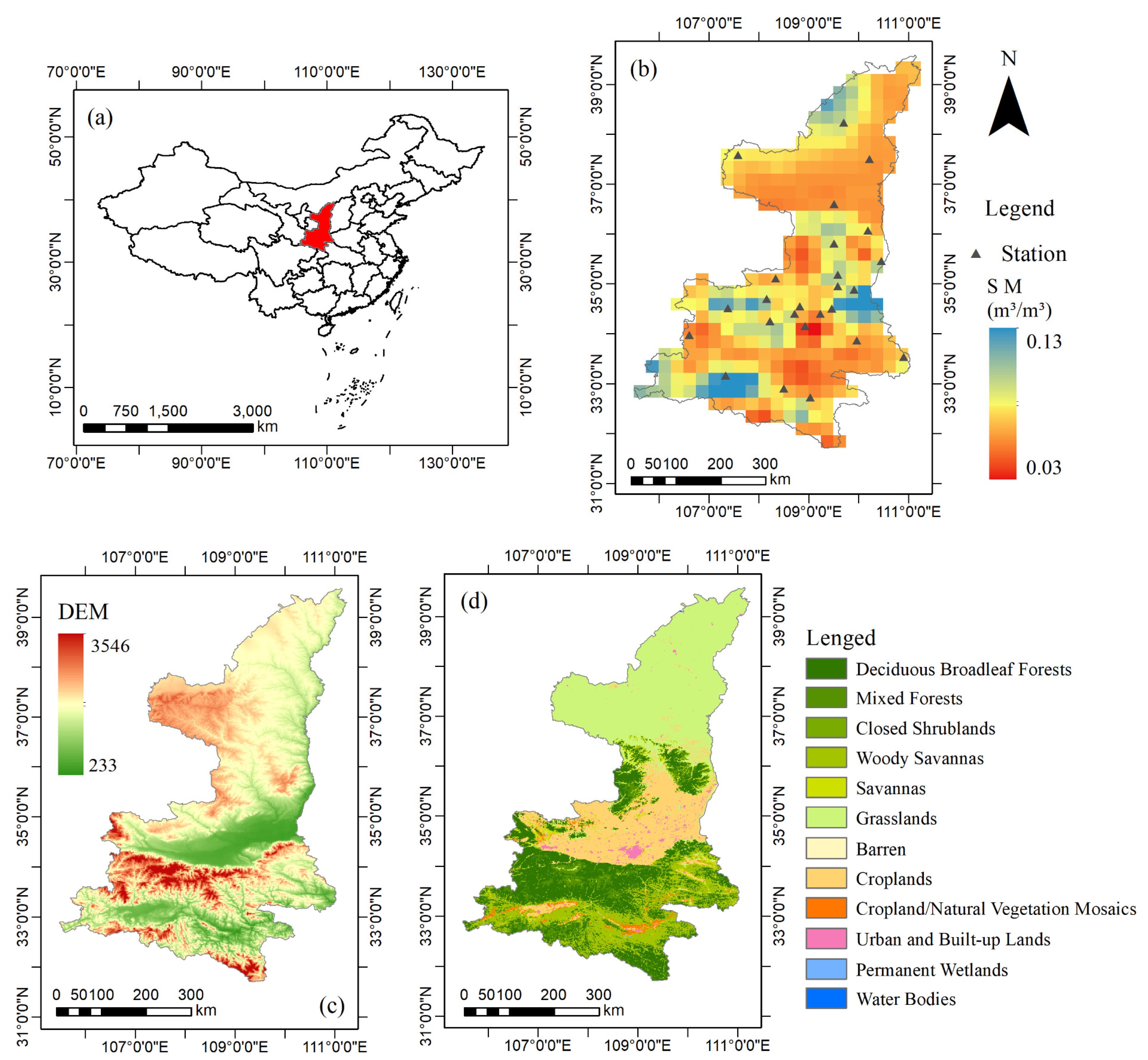
The study area selected in this paper is located in the Shaanxi Province in the interior of China, ranging from 105°29′–111°15′ E and 31°42′–39°35′ N (Figure 1). The terrain of the Shaanxi Province is high in the north and south, low in the middle, with a variety of landforms such as plateaus, mountains, plains and basins, among which the loess plateau accounts for 40% of the land area of the province. Northern and central Shaanxi have a temperate monsoon climate, but due to the difference in rainfall, the northern part is a semi-arid region, while the central part is a semi-humid region. Southern Shaanxi has a humid subtropical monsoon climate. The average annual precipitation is 340–1240 mm, with more precipitation in summer and autumn, less in winter and spring. Under the influence of climate and other conditions, the soil moisture in the Shaanxi Province is higher in the south and lower in the north, higher in summer and lower in winter.
The ground measured data are from the China meteorological data network (available online: http://www.nmic.cn/). There are 25 ground data stations, mostly distributed in low-elevation plains and valley areas, containing soil moisture data at various depths (10, 20, 40 cm). The ground data stations record soil relative humidity. Due to the lack of SM monitoring measurements at 5 cm, we chose soil moisture relative humidity data at a depth of 10 cm, as in past research [16,19,40]. Although the measurement depths are inconsistent, there is a strong correlation between the SM values of the two continuous soil layers [16,41]. The time range was from 2002 to 2013. Since the units of measured data and remote sensing data are different, and we lack the measured variables for the conversion of the two units, we can only conduct qualitative analysis of the two, but not quantitative analysis.
2.2. AMSR-E and AMSR2 Soil Moisture Products
AMSR-E is a passive microwave radiometer mounted on the Aqua satellite launched by National Aeronautics and Space Administration (NASA). It has six frequency bands of 6.925, 10.65, 18.7, 23.8, 36.5, and 89.0 GHz. The satellites, with ascending (1:30 p.m.) and descending (1:30 a.m.) modes have a revisit period of 1–2 days. At present, the derived soil moisture products of AMSR-E are obtained by three algorithms, one is created by the United Stands Snow and Ice Data Center (NSIDC) algorithm, another is created by the Japan Aerospace Exploration Agency (JAXA) algorithm and the other one is created by the Land Parameter Retrieval Model (LPRM) developed by the VU University Amsterdam with NASA. The JAXA product shows better performance under dry conditions [42]. Considering that most of the study area is non-humid, we chose the L3 soil moisture product from JAXA (http://gcom-wl.jaxa.jp/product-download.html). The spatial resolution of these data is 25 × 25 km, and the data are stored in an ease-grid format. The time coverage range is from June 2002 to September 2011, and the value range is 0–0.6 m3/m3.
AMSR2 is a passive microwave radiometer carried on the GCOM-W1 satellite launched by JAXA. Launched in July 2012, AMSR2 has continued AMSR-E’s earth observation work well until now. Compared with AMSR-E, AMSR2 adds a channel with a frequency of 7.3 GHz, which reduces the impact of radio frequency interference (RFI). In order to maintain the continuity of the data, this article also chose the AMSR2 L3 level of soil moisture product with a spatial resolution of 25 × 25 km provided by JAXA, and the time coverage is from July 2012 to August 2017.
Considering that the two sensors AMSR-E and AMSR2 are slightly different, we conducted regression analysis on the two sets of soil moisture data and obtained R2 of 0.703. The significance test proved that the two sets of product data had a good correlation within the Shaanxi Province.
2.3. Multi-Source Remote Sensing Data
Land surface temperature (LST), vegetable index (VI), evapotranspiration (ET), and land cover (LC) data were collected from NASA Moderate Resolution Imaging Spectroradiometer (MODIS). In VI, we selected two indexes, normalized differential vegetation index (NDVI) and enhanced vegetation index (EVI). The data can be downloaded from NASA’s website (http://ladsweb.nodaps.eosdis.nasa.gov/). The data information is shown in Table 1, and the time range is from June 2012 to August 2017.
The precipitation data were obtained from the Rainfall products of the Tropical Rainfall Measuring Mission (TRMM), a satellite jointly launched by NASA and JAXA in 1997 to monitor rainfall over the tropics. The satellite precipitation data used in this paper were the 3b43 monthly precipitation data set provided by NASA, which can be downloaded from the official website of NASA (http://mirador.gsfc.nasa.gov/). The spatial resolution of the data is 25 × 25 km, and the accuracy is better than that of similar satellite precipitation data. The time range is from June 2002 to August 2017.
Digital elevation model (DEM) data were acquired from the Shuttle Radar Topography Mission (SRTM) data products (http://srtm.csi.cgiar.org/SELECTION/inputCoord.asp) [43]. DEM data with a spatial resolution of 1 km were selected. Slope data and aspect data with a spatial resolution of 1 km were generated through the slope and aspect toolbars in ArcGIS 10.7 based on DEM data.
2.4. Soil Texture
Soil texture data were downloaded from the Chinese Resource and Environment Data Cloud Platform (http://www.resdc.cn/data.aspx?DATAID=260). The soil texture is divided into sand, silt, and clay. Soil texture data contains the percentage content of each category, with a spatial resolution of 1 km.
3. Methods
3.1. Machine Learning
3.1.1. Random Forest
RF is an optimized decision tree algorithm based on Bootstrap’s sampling method. The decision ability of the RF model depends on each classification and regression tree (CART). The decision tree is composed of root nodes, child nodes, and leaf nodes. Each child node contains a judging rule and the result is determined by the voting score of each decision tree. When RF is used for regression, the minimum mean square error (%) (%IncMSE) is used to calculate the regression accuracy. As for classification, the Gini index is the index to calculate the classification accuracy. The smaller Gini index refers to the less uncertainty of the model and the better classification results. RF has the advantages of high learning efficiency, insensitivity to outliers, and prevention of over-fitting. RF also has an importance analysis function for input features. The importance ranking of different factors can be obtained through the indicators %IncMSE and IncNodePurity. The calculation criteria of the two indicators are slightly different, but the results are roughly the same. %IncMSE refers to the increase value of the mean square error rate of the model after removing an impact factor. The higher %IncMSE means that the removed impact factor is more important. IncNodePurity refers to the increase of node purity after adding an impact factor. The increase in node purity means a decrease in the Gini index, and the model is better. Compared with IncNodePurity, %IncMSE is more suitable for the regression model, so this paper mainly refers to this index.
3.1.2. Support Vector Machine
SVM can be used for classification or regression. When SVM is used for classification, the principle is to find one or a group of hyperplanes based on the training sample space. The longer the distance between the training samples and the hyperplanes is, the higher the classification accuracy is. When SVM is used for regression, it is called support vector regression (SVR). We look for a regression model f(x) which is as close as possible to the actual y value when applying SVR. In contrast to the traditional regression model, SVR allows f(x) to have a certain difference from the actual y value. A threshold is set for the deviation, and the predictions within the threshold are considered correct.
3.1.3. K-Nearest Neighbor
KNN is a simple and effective machine learning algorithm. If the k-most-adjacent samples in the eigenspace belong to a certain group, then the unclassified sample also belongs to that group and has the characteristics of that group. The classification results depend on the value of k. The category of sample is only determined by the category of the nearest one or several. Compared with other algorithms, the KNN method lacks the training process.
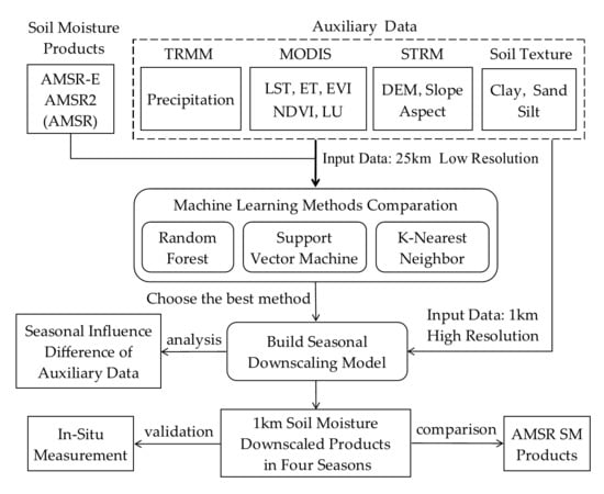
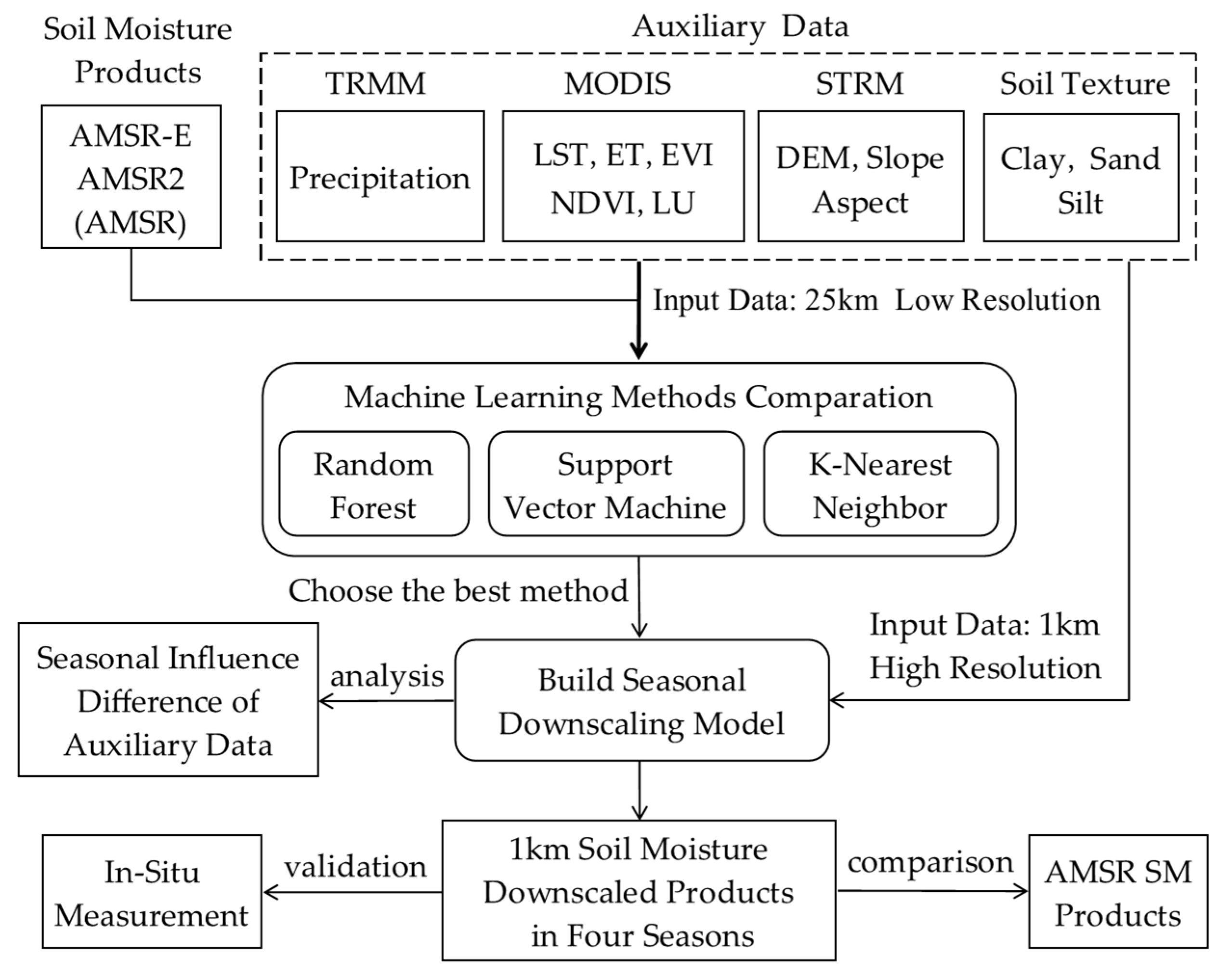
3.2. SM Product Machine Learning Downscaling
According to the climatic conditions in the study area, time spans are divided into spring (March, April, May), summer (June, July, August), autumn (September, October, November), and winter (December to February of the following year). In this study, we assume that the functional relationships between soil moisture and other auxiliary factors do not change with spatial scale, that is, in one season the functional relationship expressed in Equations (1) and (2) is the same.
Therefore, the functional relation obtained from soil moisture data and auxiliary factors on the 25 km scale can be applied to the data on the 1 km scale. The 1 km soil moisture data can be predicted by taking the data of 1 km auxiliary factors into the functional relationship. The specific downscaling steps are as follows (Figure 2).
First step: The auxiliary factors data were resampled to the spatial resolution of 25 km. The temporal resolution is different for soil moisture data and auxiliary factors data. There is constant change in different months of one season among soil moisture, meteorology, and vegetation factors. In view of this, for soil moisture, precipitation, LST, ET, and EVI, NDVI, the temporal resolution is unified as the monthly scale rather than the seasonal scale. In order to maintain the same temporal resolution, LC, terrain, and soil texture data are also unified on a monthly scale. In fact, LC remains unchanged for the same year. In addition, the value of terrain and soil texture keeps constant over the time range of this study. Finally, the sample includes three months of monthly data for one seasonal model. Take spring for example, the sample is composed of the data from March to May which benefits in the accuracy of functional relationship.
Second step: The total sample size of each season was slightly different. The sample data were randomly divided into training set and verification set, and the ratio of training sample to verification sample was about 7:3 (Table 2). The regression relationship between soil moisture and auxiliary factors under the spatial resolution of 25 km was obtained by three machine learning methods in different seasons, and the model accuracy was calculated. Then, the importance function in the random forest algorithm can be used to get the importance ranking of explanatory variables in different seasonal models. The corresponding %IncMSE value of each variable can be obtained through this function.
Third Step: The auxiliary factors data were resampled to the spatial resolution of 1 km, and all the data were processed on a seasonal scale. The seasonal data of 1 km auxiliary factors were put into different seasonal models to obtain the seasonal SM products of 1 km.
3.3. Validation Methodology
The downscaling results are evaluated and verified in three areas. First of all, the model precision evaluation of three scaling algorithms was carried out to determine the best performance of the algorithm. Secondly, the downscaling products was compared with the original 25 km soil moisture products. Finally, the in-situ measurements were used to verify the downscaling products and the original 25 km soil moisture products.
The evaluation indicators we used are the Mean Absolute Percentage Error (MAPE), BIAS, Root Mean Square Error (RMSE), Goodness of Fit (R2), Correlation Coefficient (R), and Kullback-Leibler (K-L). The equations for the indicators are shown as follows (Equations (3)–(8)). Several statistical parameters including MAPE, BIAS, RMSE, and R2 were used to compare the downscaling models obtained by different machine learning algorithms. The MAPE, BIAS, and RMSE were used for the comparisons between the 1 km downscaled products and the original 25 km soil moisture products. For direct validation, the downscaled results were verified with the in-situ measurements using the R and the K-L.
where and represent different values in different evaluation parts. means the predicted values or downscaled data, and stands for the validation data or true values. is the covariance of and , is the covariance of , is the covariance of .
4. Results
4.1. Comparative Analysis of Machine Learning Algorithms
We evaluated the accuracy of the downscaling models, and the results are shown in Table 3. In general, the model accuracy of the three algorithms is acceptable. The MAPE value is less than 24%, and BIAS is less than 0.065 m3/m3, and the RMSE value is not more than 0.027 m3/m3. According to the R2, the correlation between the RF predicted value and the true value is the highest, and the highest value is 0.609 in autumn. The variation range of SM values in different seasons may have an impact on R2. RF performs well in terms of MAPE, RMSE, and R2, but poorly in BIAS. The autumn results are used for further analysis. The BIAS of RF is 0.041 m3/m3 in autumn which is much higher than that of SVM and KNN. However, the MAPE and RMSE of RF are the smallest, and the R2 is the highest. We conclude that the RF-predictions are mainly overestimated rather than underestimated compared with other algorithms, and the deviation is relatively low. The overestimation and underestimation of the other two algorithms are more evenly distributed, and the deviation value is larger.
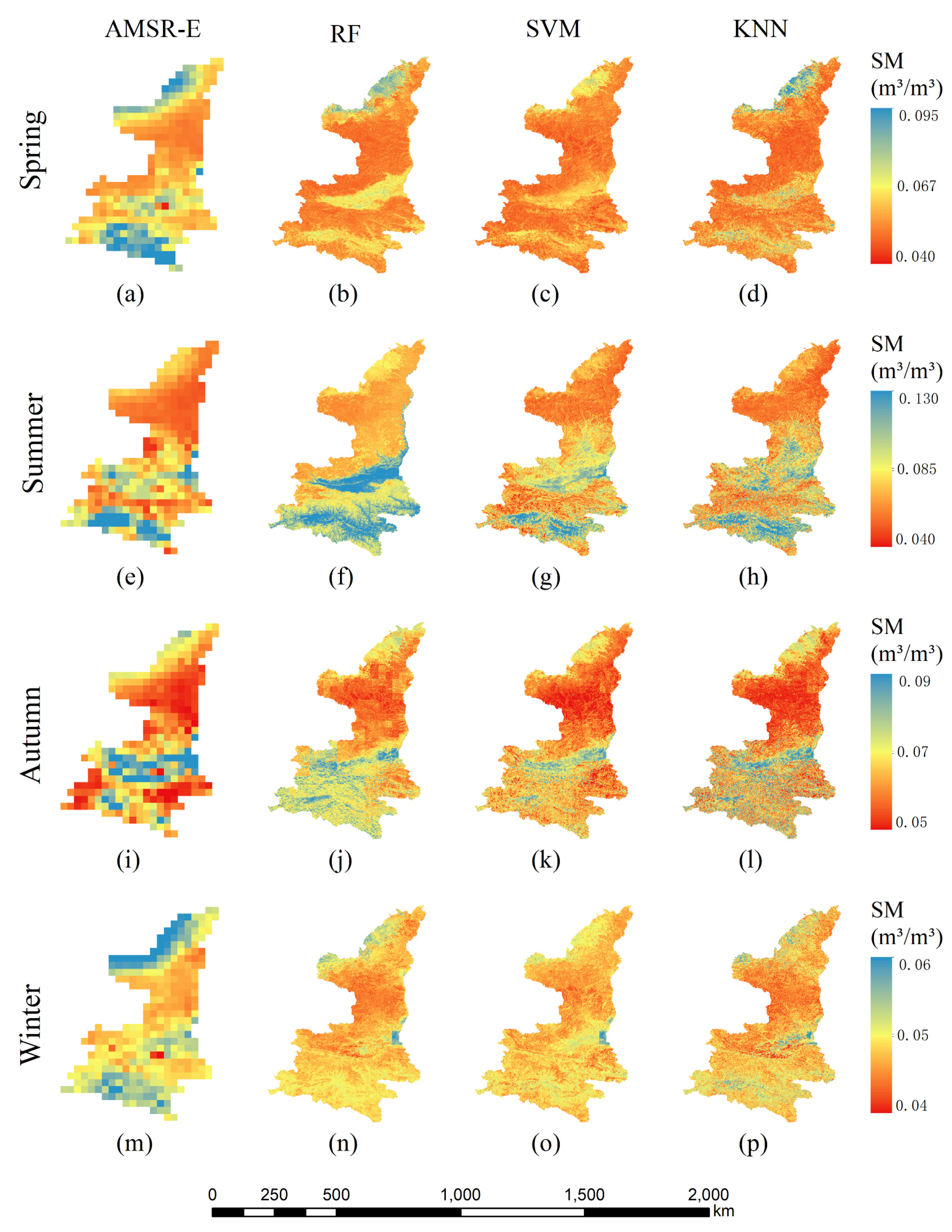
Combined with Figure 3, we can find that the spatial distribution of the downscaled results obtained by the three algorithms is generally consistent. The RF result in summer is higher compared to other algorithms, which is consistent with the BIAS index. In addition, in the figures of spring and summer, the soil moisture smoothing effect obtained by RF in the middle research area is not as good as that obtained by SVM. In general, SVM performs moderately, and slightly worse than the RF algorithm. The KNN results show that there are high and low values cross distribution, especially in the central and southern regions in summer and autumn, and there is no smooth values transition. It may have relevance for the algorithm execution rules. The KNN algorithm only takes into account the surrounding range of values when making predictions. This may also be the reason for the poor performance of KNN algorithm. Since RF is the best among the three algorithms, we choose RF for downscaling in the following process.
4.2. Effectiveness of Seasonal Downscaling Model
In order to prove the effectiveness of the seasonal downscaling model, we built a comprehensive downscaling model without distinguishing seasons for a comparison experiment. The training samples of the four seasons in Table 2 were mixed, and 9979 samples were randomly selected to train a comprehensive downscaling model. Then, the same validation samples as those in Table 2 were selected to verify the accuracy of the comprehensive model in each season. The results are shown in Table 4.
The comparison results included MAPE, BIAS, RMSE, and R2. It can be seen that the MAPE, BIAS, and RMSE from the seasonal model are lower than the comprehensive model, especially in spring and winter. According to the performance of R2, the fitting degree between the predicted results of the seasonal model and the verification samples is better. We calculated the magnitude of the improvement of model accuracy after considering season differences. On average, the MAPE, BIAS, and RMSE decreased by 17%, 28%, and 10%, respectively, using the season-based methods. In addition, R2 improved by an average of 13%. The value of BIAS of the season-based model in winter decreased a lot, so the average reduction rate of BIAS was relatively high. Overall, the accuracy of the downscaling model improved by about 10% while considering seasonal differences. The results demonstrate that the seasonal model performs better than the comprehensive model.
4.3. Evaluation of Downscaled Products
4.3.1. Comparison with Original AMSR-E/AMSR2 Soil Moisture
As shown in Figure 3, taking 2010 for example, the RF-downscaled results are roughly consistent with the spatial distribution of the original products of 25 km. The soil moisture values show a decreasing trend from south to north. In addition, the soil moisture downscaled result represents more detailed spatial distribution and smoother spatial variation. Especially in Qinling Mountains, it is easier to identify mountains and the plains between mountains, and the variation of soil moisture with the topography is also well represented. Although there are some deviations in some areas, the downscaled results are acceptable considering the complex and varied topography and climate of the study area.
We resampled the original SM products to a spatial resolution of 1 km. The 1 km SM data after resampling maintain the SM value at 25 km scale. Then, we compared the downscaled products with the resampled products to obtain the difference between them at 1 km scale (Table 5). The maximum RMSE value is 0.024 m3/m3 in summer, 0.013 m3/m3 in autumn, and lower than 0.010 m3/m3 in spring and winter. Except for the autumn, all the other three seasons have negative BIAS. It indicates that compared with the original soil moisture of 25 km, the soil moisture value after downscaling is low. The maximum value of MAPE is 34% in summer, which is slightly higher. The MAPE value is between 10%–20% in spring and autumn, and within 10% in winter.
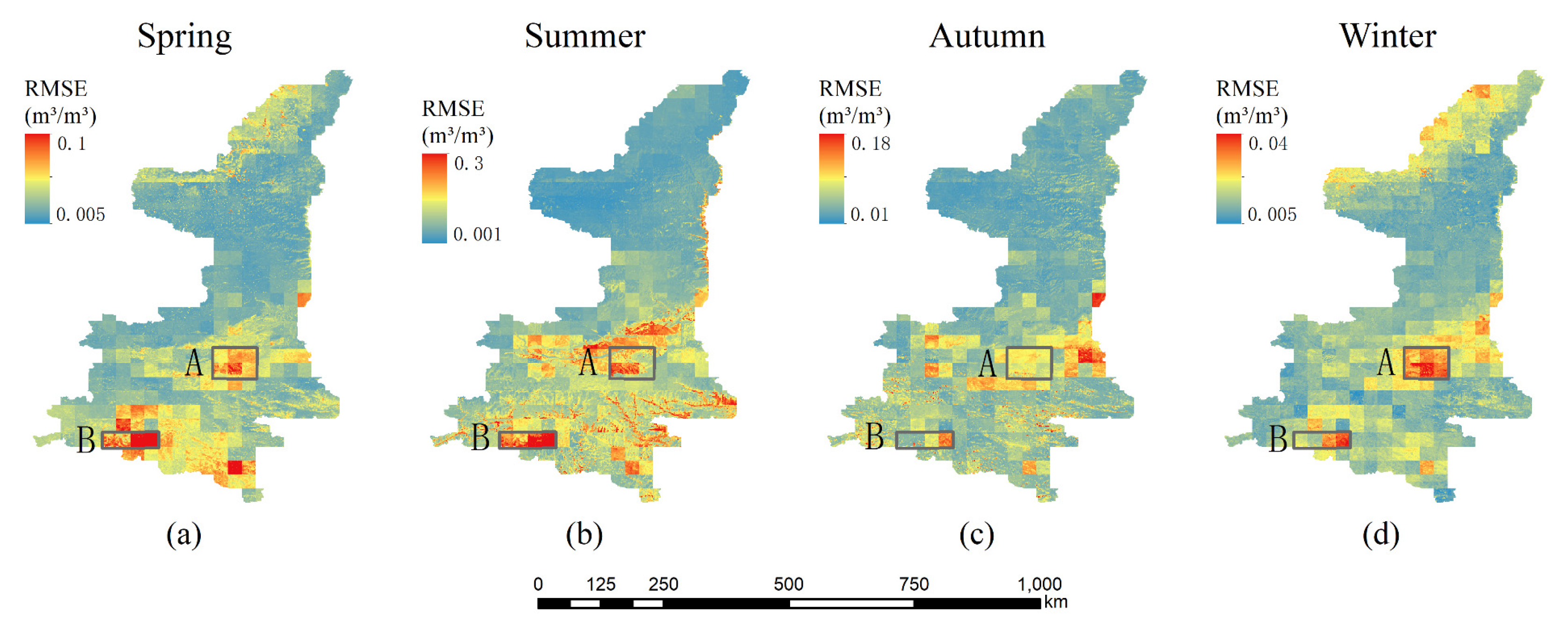
Figure 4 shows the spatial distribution of RMSE with seasons. To illustrate the difference between the original data and the downscaled result, we selected region A and B for analysis. Compared with the original SM value, the downscaled SM value of region A is higher, while the downscaled SM value of region B is lower. Most of region A belongs to urban and built-up areas. The NDVI value in this region is lower than that in the surrounding areas, but the meteorological and topographical differences between this region and surrounding areas are not significant. Therefore, overestimation may occur under the guidance of topographic and meteorological factors. In addition, fewer urban ground stations are used for sensor calibration in the generation stage of SM products [44]. Urban areas are rarely considered in the comparative validation of SM products [45,46]. These may affect the accuracy of remote sensing SM products in the urban areas. Therefore, the possibility of low accuracy of the original 25 km SM products cannot be ruled out. Region B is located in the transition from mountains to valley plains. The climate and vegetation coverage in region B are very similar to that of the surrounding areas. In the original 25 km resolution SM products, it is the place with the highest soil moisture value in the study area, but not after downscaling. Region B has the highest soil moisture value in the original 25 km data, and it may be related to other factors such as proximity to rivers and reservoirs.
It can be seen from Figure 5 that the downscaled soil moisture values maintain a good consistency with the original 25 km data. However, we also noted that the SM value of AMSR2 is slightly lower than the AMSR-E value. Therefore, the time continuity of soil moisture products was also improved after downscaling.
4.3.2. Comparison with In-Situ Measurements
We unified the temporal resolution of the in-situ measurements data to the seasonal scale. Since the units of downscaled data and measured data are different, the data were normalized according to the maximum and minimum values before the comparative analysis. We verified original 25 km SM products and downscaled products by R and K-L indexes. The higher R value or the smaller K-L means a better result. After excluding the outliers in the measured data, the number of samples used for data analysis in spring, summer, autumn, and winter were 167, 180, 137, and 89, respectively.
According to Table 6, we can see that the R values of the downscaled data and measured data are increased to 0.570, 0.458, 0.764, and 0.288, respectively for the four seasons, which are higher than that of the original 25 km data and measured data. The small correlation between remote sensing data and ground measurements may be due to their differences in the spatial support [21]. The K-L values of the original 25 km data and the measured data for the four seasons are 0.143, 0.305, 0.222, and 0.080, while the K-L values of the downscaled data and the measured data are reduced to 0.084, 0.236, 0.221, and 0.075. The correlation or fitting degree between the downscaled data and the measured data is better and the difference is smaller. These results prove the effectiveness of the downscaling. In winter, the difference between the downscaled data and the measured data is the smallest according to the K-L value, but the R value is the lowest, which may be caused by the small range of soil moisture variation.
4.4. Seasonal Difference Analysis of Explanatory Variables
We got the ranking of explanatory variables with seasons at 25 km spatial resolution using the importance function of random forest (Table 7). The ranking results are verified by correlation analysis. Explanatory factors all passed the significance tests, and the correlations with soil moisture were strong. The R2 value between the factor with the largest %IncMSE and SM was also the highest.
Since the variables contained in the downscaling models of the four seasons are the same, we can assume a unified threshold to judge the importance of factors. When the value of %IncMSE exceeds 100, we assume that this factor has a greater impact on soil moisture. The main factors affecting soil moisture are different with seasons. Precipitation, elevation, land surface temperature, and slope all have an impact on soil moisture in spring. Soil moisture is mainly affected by elevation, precipitation, aspect, and land surface temperature in summer. Precipitation and aspect have a great influence on soil moisture in autumn while the influence of precipitation, NDVI, and LST is significant in winter. These results show the seasonal effect between soil moisture and auxiliary factors, and proves the necessity of establishing seasonal models.
We analyzed the seasonal differences of the main influencing factors according to their categories. Summer is mainly influenced by meteorological and topographic factors. There is the southeast monsoon prevailing in summer, brining heavy rainfall. Affected by topographical factors, the land surface temperature in Shaanxi is high in summer and the evapotranspiration is strong. Topography usually affects the spatial distribution of SM in wet conditions [35], especially during and immediately after a rainfall event [47]. In addition, elevation also plays a role in divisions of study area because of an obvious height difference between them. The central plains and the southern valley plains receive more precipitation than other regions, resulting in higher soil moisture values. Therefore, topographic factors not only directly affect the spatial distribution of soil moisture content, but also further affect soil moisture by influencing meteorological factors.
In spring and autumn, the main factors affecting soil moisture are all meteorological factors and topographic, but the value of %IncMSE corresponding to these factors varies greatly. The difference of %IncMSE of different factors in spring is close, while the value of %IncMSE of meteorological and topographic factors in autumn is obviously very high. Compared with autumn, meteorological conditions are less variable in spring with lower precipitation and less frequency of rainfall. In addition, precipitation in September is at a high level and the monsoon effects still exist.
Soil moisture in winter is mainly affected by meteorological factors and vegetation. In winter, meteorological factors become less active due to low temperature and little rain. Thus, the properties of the soil itself become more important. The level of soil moisture depends less on external supplies and more on the ability of the soil to retain moisture.
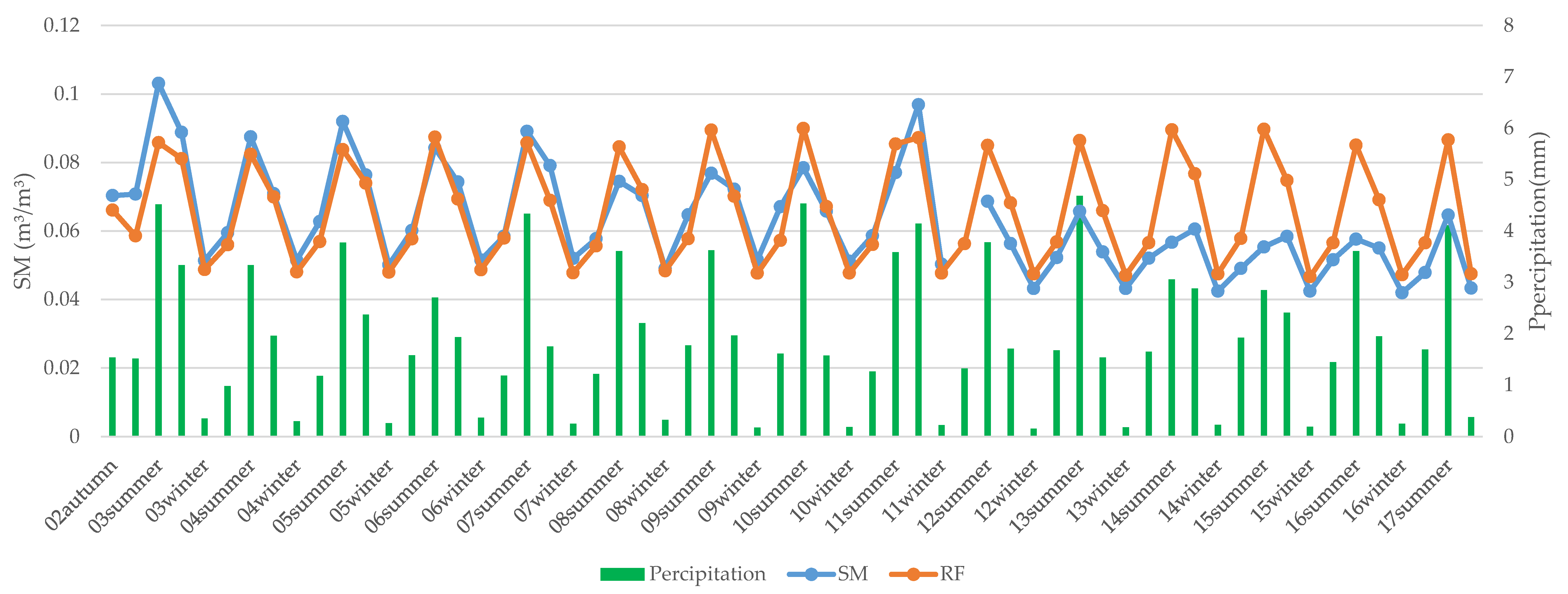
According to the performance of different auxiliary factors in each season, precipitation is the key factor affecting soil moisture. In previous studies, although the time-continuous variation trend of precipitation and soil water value was compared, precipitation was rarely directly used as an influencing factor to participate in modeling. One reason is that the spatial resolution of precipitation products is relatively coarse. Another is that there may be a time hysteresis effect between soil moisture and precipitation. The occurrence of rainfall is on a large scale. It can be implied that the impact of coarse resolution precipitation products is relatively small. In general, the soil depth in remote sensing data is generally around 5 cm, because the microwave penetrates the soil up to 5 cm. There is no time lag between soil moisture and precipitation at this depth at seasonal scale. According to Figure 5, the change trend of soil moisture is roughly the same as that of precipitation. Some extreme soil moisture values are accompanied by extreme rainfall values.
Among the topographic factors, elevation, slope, and soil moisture are negatively correlated. There is lower temperature and less precipitation due to high altitude. What is more, direct sunlight leads to higher evapotranspiration. Sandy soil and less vegetation aggravate the situation. Obviously, it is not easy to retain soil moisture under these conditions. Water flows from high to low by gravity, and steep slopes speed up the flow of water, leaving steeper areas with less water to preserve. Although the influence of aspect on each season is different, they all show similar laws. The soil moisture on the south and north aspect is higher. The north slope is an overcast slope with low solar intensity, low surface temperature and low evaporation, so soil preserves water well. Although the south slope is a sunny slope, it is also towards the southeast monsoon with sufficient precipitation supply.
According to the %IncMSE value, sandy, clay, and silt have little influence on the establishment of the model. We tested on the removal of soil texture from the downscaling model in summer and winter. The model comparison suggested that although soil texture is a less important predictor, the model performed better when soil texture is included (Table 8).
5. Discussion
Soil moisture is a key factor in agriculture research, but the spatial resolution of current products is insufficient to meet research needs. The variation of SM is a complex and synthetic process, which is impacted by numerous factors [19]. In recent years, more attention has been paid to the influence of spatial heterogeneity rather than temporal heterogeneity in the research on improving the spatial resolution of soil moisture remote sensing products. This is often overlooked in downscaling studies of factors that change dynamically over time. The significant improvement in this study is to mainly consider the influence of time heterogeneity on soil moisture downscaling. In a study area with four distinct seasons, we divided the time periods according to the seasons. A variety of explanatory variables involving meteorology, topography, land cover, and soil properties were selected in the establishment of the downscaling model. In addition, this model can be built more accurately with the help of machine learning methods.
We verified whether the accuracy of the downscaling model can be improved after considering the seasonal difference. The results in Table 4 support our argument. In addition, it can also be seen from Table 7 that the influence degree of explanatory variables on soil moisture is different in each season. That is to say, the relationship between soil moisture and auxiliary factors also has a large seasonal difference. These mean that seasonal differences do affect results and should be considered in relevant studies. Compared with the original remote sensing data, summer downscaled results have the largest deviation in four seasons (MAPE = 34%, RMSE = 0.024 m3/m3, BIAS = −0.019 m3/m3). The downscaled product has better correlation with the in-situ measurements than the original remote sensing product. According to the evaluation results of the downscaled SM products, the performance of winter products is the best, while the performance of summer products is slightly inadequate. Having got the downscaled results, how to reduce the deviation in summer is the focus of the future research. The performance of the downscaled products in different seasons is positively correlated with the soil moisture stability. The better the stability of soil moisture value is, the better the downscaled result is. In summer, there is drastic change in meteorological factors. Precipitation, land surface temperature, and evapotranspiration intensity all reach the highest values in a year, bringing high moisture supply to the soil and strong evapotranspiration at the same time. The vegetation cover types in the study area are mostly deciduous. Summer is the period when the difference in vegetation coverage between different land cover types is the largest. High vegetation coverage reduces the accuracy of the sensor in obtaining soil moisture information, and the spatial heterogeneity of the mixed pixels is greatly enhanced. Thus, soil moisture values in summer are very unstable and affected by meteorological and vegetation factors. We also take into account that the deviation of the original remote sensing soil moisture products in summer is likely to be the largest, and there would be a deviation transfer in the downscaling process. In contrast, soil moisture values in winter are at a relatively low and stable level because of low temperature, little rain, and low vegetation coverage. In this study area, the rainfall in autumn is greater than that in spring, and the soil moisture values are also higher and more unstable in autumn. Therefore, the downscaling results in spring are better than in autumn.
In this study, the same input explanatory variables were used in the establishment of the seasonal downscaling model. In the following research, the most suitable downscaling model for each season can be determined according to the importance of explanatory variables. In addition to the auxiliary data selected in this study, we can also consider the infrared data [24,48] and SAR [7,16,18]. Additionally, we chose the seasonal scale for research, since the climate in the study area has four distinct seasons. However, this time division is not applicable to tropical or cold regions. We can divide different time scales according to the condition of the research area and the research emphasis. For example, dry and wet seasons can be distinguished in tropical monsoon regions, and growing seasons and non-growing seasons can be distinguished in the research based on cultivated land.
Due to the lack of measured data of unit conversion, the in-situ measurements used for verification in this paper are not consistent with the unit of remote sensing data. In addition, there is no soil moisture data with a depth of 5 cm in the ground monitoring stations, so the soil moisture values with a depth of 10 cm are mostly used in the experiments. What is more, the in-situ measurements are at point scale, while remote sensing products are at the 1-km-pixel scale. In the study of verifying remote sensing data with measured data, there is always unreasonable matching in the space scale [20]. These factors may all affect the accuracy of validation. Therefore, it is necessary to explore other effective validation methods to evaluate downscaled SM products [19].
We compared the three machine learning methods in order to get the most suitable method for this research. According to their performance, the random forest has the best comprehensive performance. The RF-downscaled products have superior matching performance to both AMSR SM products and in-situ measurements. However, RF still has some shortcomings, such as overall overestimation. The method would be optimized by adjusting parameters to make it more suitable for our study. In addition to the machine learning method used in this paper, other algorithms such as neural networks [17,38] and Bayesian [49] have also been used in the downscaling research. The comparison and integration of different algorithms can also be a focus of future research.
6. Conclusions
In this paper, we have proved that season-based downscaling is even better than continuous time series. The AMSR SM products were downscaled based on the machine learning method. The relationship between meteorology, topography, land cover types, and soil properties was considered in the model. We finally obtained 1 km soil moisture products from 2002 to 2017 on a seasonal scale in the Shaanxi province. The downscaled products not only maintain the accuracy of AMSR-E/AMSR2 SM products, but improves the time continuity of the SM products. Compared with the original 25 km products, the downscaled results have a higher fitting degree with the in-situ measurements, providing more abundant spatial information of soil moisture. Through the research of this paper, we get the following conclusions:
- (1)
- Three machine learning methods RF, SVM, and KNN were selected to construct downscaling models. By comparing the accuracy of the downscaling models, we found RF performs best. One deficiency of RF is overestimation.
- (2)
- The construction of the downscaling model with seasons can improve the accuracy. Season-based downscaling is effective. The winter downscaled result is the best, as the characteristics of soil moisture in winter are in a relatively stable state with low content and small variation.
- (3)
- The influence of different factors on soil moisture varies with seasons, but precipitation is a key factor for all four seasons. For summer and autumn, the influence of meteorological factors and topographic factors on soil moisture is very prominent. However, vegetation is more prominent in winter.
In this study, the influence of seasonal differences is considered in the process of downscaling. This provides a new perspective for the study of soil moisture or other dynamic variables. In terms of explanatory variables for the establishment of the downscaling model, we chose four types of factors and analyzed the seasonal differences of their influence on soil moisture. Our analysis can provide reference for subsequent studies on soil moisture.
Author Contributions
The research topic was designed by R.Y.; J.B. and R.Y. performed the research and wrote the manuscript; J.B. checked the experimental data, examined the experimental results, and participated in the revision of the manuscript. All authors have read and agreed to the published version of the manuscript.
Funding
This research was funded by the key research and development program of Shaanxi province (grant No: 2020NY-166). And the APC was funded by the key research and development program of Shaanxi province (grant No: 2020NY-166).
Acknowledgments
We are indebted to the National Aeronautics and Space Administration and the United States Geological Survey for providing MODIS, DEM, and TRMM data, Japan Aerospace Exploration Agency for providing AMSR-E/AMSR2 SM data, China Meteorological Science Data Sharing Network for providing in-situ measurements, and Chinese Resource and Environment Data Cloud Platform for providing soil texture data. Furthermore, we are very grateful for the machine learning algorithms packages provided by the R software to allow reproducibility of the workflow. In addition, we are grateful for the valuable feedback from the anonymous reviewers.
Conflicts of Interest
The authors declare no conflict of interest.
References
- Ochsner, T.E.; Cosh, M.H.; Cuenca, R.H.; Dorigo, W.A.; Draper, C.S.; Hagimoto, Y.; Kerr, Y.H.; Larson, K.M.; Njoku, E.G.; Small, E.E.; et al. State of the Art in Large-Scale Soil Moisture Monitoring. Soil Sci. Soc. Am. J. 2013, 77, 1888–1919. [Google Scholar] [CrossRef] [Green Version]
- Seneviratne, S.I.; Corti, T.; Davin, E.L.; Hirschi, M.; Jaeger, E.B.; Lehner, I.; Orlowsky, B.; Teuling, A.J. Investigating soil moisture–climate interactions in a changing climate: A review. Earth Sci. Rev. 2010, 99, 125–161. [Google Scholar] [CrossRef]
- Engman, E.T. Applications of microwave remote sensing of soil moisture for water resources and agriculture. Remote Sens. Environ. 1991, 35, 213–226. [Google Scholar] [CrossRef]
- Corradini, C. Soil moisture in the development of hydrological processes and its determination at different spatial scales. J. Hydrol. 2014, 516, 1–5. [Google Scholar] [CrossRef]
- Albergel, C.; de Rosnay, P.; Gruhier, C.; Muñoz-Sabater, J.; Hasenauer, S.; Isaksen, L.; Kerr, Y.; Wagner, W. Evaluation of remotely sensed and modelled soil moisture products using global ground-based in situ observations. Remote Sens. Environ. 2012, 118, 215–226. [Google Scholar] [CrossRef]
- Njoku, E.G.; Entekhabi, D. Passive microwave remote sensing of soil moisture. J. Hydrol. 1996, 184, 101–129. [Google Scholar] [CrossRef]
- Li, J.; Wang, S.; Gunn, G.; Joosse, P.; Russell, H.A.J. A model for downscaling SMOS soil moisture using Sentinel-1 SAR data. Int. J. Appl. Earth Obs. Geoinf. 2018, 72, 109–121. [Google Scholar] [CrossRef]
- Jiang, H.; Shen, H.; Li, H.; Lei, F.; Gan, W.; Zhang, L. Evaluation of Multiple Downscaled Microwave Soil Moisture Products over the Central Tibetan Plateau. Remote Sens. 2017, 9, 402. [Google Scholar] [CrossRef] [Green Version]
- Njoku, E.G.; Jackson, T.J.; Lakshmi, V.; Chan, T.K.; Nghiem, S.V. Soil moisture retrieval from AMSR-E. IEEE Trans. Geosci. Remote Sens. 2003, 41, 215–229. [Google Scholar] [CrossRef]
- Keiji, I.; Takashi, M.; Misako, K.; Marehito, K.; Norimasa, I.; Keizo, N. Status of AMSR2 instrument on GCOM-W1. In Proceedings of the Asia-Pacific Remote Sensing (SPIE), Kyoto, Japan, 29 October–1 November 2012. [Google Scholar]
- Wigneron, J.P.; Waldteufel, P.; Chanzy, A.; Calvet, J.C.; Kerr, Y. Two-Dimensional Microwave Interferometer Retrieval Capabilities over Land Surfaces (SMOS Mission). Remote Sens. Environ. 2000, 73, 270–282. [Google Scholar] [CrossRef]
- Parinussa, R.M.; Wang, G.; Holmes, T.R.H.; Liu, Y.Y.; Dolman, A.J.; de Jeu, R.A.M.; Jiang, T.; Zhang, P.; Shi, J. Global surface soil moisture from the Microwave Radiation Imager onboard the Fengyun-3B satellite. Int. J. Remote Sens. 2014, 35, 7007–7029. [Google Scholar] [CrossRef]
- Entekhabi, D.; Njoku, E.G.; Neill, P.E.O.; Kellogg, K.H.; Crow, W.T.; Edelstein, W.N.; Entin, J.K.; Goodman, S.D.; Jackson, T.J.; Johnson, J.; et al. The Soil Moisture Active Passive (SMAP) Mission. Proc. IEEE 2010, 98, 704–716. [Google Scholar] [CrossRef]
- Peng, J.; Loew, A.; Merlin, O.; Verhoest, N.E.C. A review of spatial downscaling of satellite remotely sensed soil moisture. Rev. Geophys. 2017, 55, 341–366. [Google Scholar] [CrossRef]
- Atkinson, P.M. Downscaling in remote sensing. Int. J. Appl. Earth Obs. Geoinf. 2013, 22, 106–114. [Google Scholar] [CrossRef]
- Bai, J.; Cui, Q.; Zhang, W.; Meng, L. An Approach for Downscaling SMAP Soil Moisture by Combining Sentinel-1 SAR and MODIS Data. Remote Sens. 2019, 11, 2736. [Google Scholar] [CrossRef] [Green Version]
- Cui, Y.; Chen, X.; Xiong, W.; He, L.; Lv, F.; Fan, W.; Luo, Z.; Hong, Y. A Soil Moisture Spatial and Temporal Resolution Improving Algorithm Based on Multi-Source Remote Sensing Data and GRNN Model. Remote Sens. 2020, 12, 455. [Google Scholar] [CrossRef] [Green Version]
- Holtgrave, A.-K.; Foerster, M.; Greifeneder, F.; Notarnicola, C.; Kleinschmit, B. Estimation of Soil Moisture in Vegetation-Covered Floodplains with Sentinel-1 SAR Data Using Support Vector Regression. PFG J. Photogramm. Remote Sens. Geoinf. Sci. 2018, 86, 85–101. [Google Scholar] [CrossRef]
- Liu, Y.; Yang, Y.; Jing, W.; Yue, X. Comparison of Different Machine Learning Approaches for Monthly Satellite-Based Soil Moisture Downscaling over Northeast China. Remote Sens. 2017, 10, 31. [Google Scholar] [CrossRef] [Green Version]
- Zappa, L.; Forkel, M.; Xaver, A.; Dorigo, W. Deriving Field Scale Soil Moisture from Satellite Observations and Ground Measurements in a Hilly Agricultural Region. Remote Sens. 2019, 11, 2596. [Google Scholar] [CrossRef] [Green Version]
- Crow, W.T.; Berg, A.A.; Cosh, M.H.; Loew, A.; Mohanty, B.P.; Panciera, R.; de Rosnay, P.; Ryu, D.; Walker, J.P. Upscaling sparse ground-based soil moisture observations for the validation of coarse-resolution satellite soil moisture products. Rev. Geophys. 2012, 50, 372. [Google Scholar] [CrossRef] [Green Version]
- Vereecken, H.; Huisman, J.A.; Pachepsky, Y.; Montzka, C.; van der Kruk, J.; Bogena, H.; Weihermüller, L.; Herbst, M.; Martinez, G.; Vanderborght, J. On the spatio-temporal dynamics of soil moisture at the field scale. J. Hydrol. 2014, 516, 76–96. [Google Scholar] [CrossRef]
- Piles, M.; Sanchez, N.; Vall-llossera, M.; Camps, A.; Martinez-Fernandez, J.; Martinez, J.; Gonzalez-Gambau, V. A Downscaling Approach for SMOS Land Observations: Evaluation of High-Resolution Soil Moisture Maps Over the Iberian Peninsula. IEEE J. Sel. Top. Appl. Earth Obs. Remote Sens. 2014, 7, 3845–3857. [Google Scholar] [CrossRef] [Green Version]
- Piles, M.; Camps, A.; Vall-Llossera, M.; Corbella, I.; Panciera, R.; Ruediger, C.; Kerr, Y.H.; Walker, J. Downscaling SMOS-Derived Soil Moisture Using MODIS Visible/Infrared Data. IEEE Trans. Geosci. Remote Sens. 2011, 49, 3156–3166. [Google Scholar] [CrossRef]
- Piles, M.; Petropoulos, G.P.; Sanchez, N.; Gonzalez-Zamora, A.; Ireland, G. Towards improved spatio-temporal resolution soil moisture retrievals from the synergy of SMOS and MSG SEVIRI spaceborne observations. Remote Sens. Environ. 2016, 180, 403–417. [Google Scholar] [CrossRef] [Green Version]
- Alemohammad, S.H.; Kolassa, J.; Prigent, C.; Aires, F.; Gentine, P. Global downscaling of remotely sensed soil moisture using neural networks. Hydrol. Earth Syst. Sci. 2018, 22, 5341–5356. [Google Scholar] [CrossRef] [Green Version]
- Xiang, D.; Liu, L.; Wang, Q.; Yang, N.; Han, T. Evaluation of Data Quality and Drought Monitoring Capability of FY-3A MERSI Data. Adv. Artif. Intell. 2010, 2010, 124816. [Google Scholar] [CrossRef] [Green Version]
- Zhao, W.; Sanchez, N.; Lu, H.; Li, A. A spatial downscaling approach for the SMAP passive surface soil moisture product using random forest regression. J. Hydrol. 2018, 563, 1009–1024. [Google Scholar] [CrossRef]
- Im, J.; Park, S.; Rhee, J.; Baik, J.; Choi, M. Downscaling of AMSR-E soil moisture with MODIS products using machine learning approaches. Environ. Earth Sci. 2016, 75, 1120. [Google Scholar] [CrossRef]
- Han, J.; Mao, K.; Xu, T.; Guo, J.; Zuo, Z.; Gao, C. A soil moisture estimation framework based on the CART algorithm and its application in China. J. Hydrol. 2018, 563, 65–75. [Google Scholar] [CrossRef]
- Ranney, K.J.; Niemann, J.D.; Lehman, B.M.; Green, T.R.; Jones, A.S. A method to downscale soil moisture to fine resolutions using topographic, vegetation, and soil data. Adv. Water Resour. 2015, 76, 81–96. [Google Scholar] [CrossRef] [Green Version]
- Kathuria, D.; Mohanty, B.P.; Katzfuss, M. A Nonstationary Geostatistical Framework for Soil Moisture Prediction in the Presence of Surface Heterogeneity. Water Resour. Res. 2019, 55, 729–753. [Google Scholar] [CrossRef] [Green Version]
- Panciera, R.; Walker, J.P.; Kalma, J.D.; Kim, E.J.; Hacker, J.M.; Merlin, O.; Berger, M.; Skou, N. The NAFE’05/CoSMOS Data Set: Toward SMOS Soil Moisture Retrieval, Downscaling, and Assimilation. IEEE Trans. Geosci. Remote Sens. 2008, 46, 736–745. [Google Scholar] [CrossRef] [Green Version]
- Korres, W.; Reichenau, T.G.; Fiener, P.; Koyama, C.N.; Bogena, H.R.; Cornelissen, T.; Baatz, R.; Herbst, M.; Diekkrüger, B.; Vereecken, H.; et al. Spatio-temporal soil moisture patterns—A meta-analysis using plot to catchment scale data. J. Hydrol. 2015, 520, 326–341. [Google Scholar] [CrossRef] [Green Version]
- Gaur, N.; Mohanty, B.P. Evolution of physical controls for soil moisture in humid and subhumid watersheds. Water Resour. Res. 2013, 49, 1244–1258. [Google Scholar] [CrossRef]
- Joshi, C.; Mohanty, B.P. Physical controls of near-surface soil moisture across varying spatial scales in an agricultural landscape during SMEX02. Water Resour. Res. 2010, 46. [Google Scholar] [CrossRef] [Green Version]
- Kovačević, J.; Cvijetinović, Ž.; Stančić, N.; Brodić, N.; Mihajlović, D. New Downscaling Approach Using ESA CCI SM Products for Obtaining High Resolution Surface Soil Moisture. Remote Sens. 2020, 12, 1119. [Google Scholar] [CrossRef] [Green Version]
- Srivastava, P.K.; Han, D.; Ramirez, M.R.; Islam, T. Machine Learning Techniques for Downscaling SMOS Satellite Soil Moisture Using MODIS Land Surface Temperature for Hydrological Application. Water Resour. Manag. 2013, 27, 3127–3144. [Google Scholar] [CrossRef]
- Park, S.; Im, J.; Park, S.; Rhee, J. Drought monitoring using high resolution soil moisture through multi-sensor satellite data fusion over the Korean peninsula. Agric. Meteorol. 2017, 237–238, 257–269. [Google Scholar] [CrossRef]
- Peng, J.; Loew, A.; Zhang, S.; Wang, J.; Niesel, J. Spatial Downscaling of Satellite Soil Moisture Data Using a Vegetation Temperature Condition Index. IEEE Trans. Geosci. Remote Sens. 2016, 54, 558–566. [Google Scholar] [CrossRef]
- Kędzior, M.; Zawadzki, J. Comparative study of soil moisture estimations from SMOS satellite mission, GLDAS database, and cosmic-ray neutrons measurements at COSMOS station in Eastern Poland. Geoderma 2016, 283, 21–31. [Google Scholar] [CrossRef]
- Kim, S.; Liu, Y.Y.; Johnson, F.M.; Parinussa, R.M.; Sharma, A. A global comparison of alternate AMSR2 soil moisture products: Why do they differ? Remote Sens. Environ. 2015, 161, 43–62. [Google Scholar] [CrossRef]
- Farr, T.G.; Rosen, P.A.; Caro, E.; Crippen, R.; Duren, R.; Hensley, S.; Kobrick, M.; Paller, M.; Rodriguez, E.; Roth, L.; et al. The Shuttle Radar Topography Mission. Rev. Geophys. 2007, 45. [Google Scholar] [CrossRef] [Green Version]
- Koike, T.; Nakamura, Y.; Kaihotsu, I.; Davaa, G.; Matsuura, N.; Tamagawa, K.; Fujii, H. Development of an Advanced Microwave Scanning Radiometer (AMSR-E) algorithm for soil moisture and vegetation water content. Annu. J. Hydraul. Eng. Jpn. Soc. Civ. Eng. 2004, 48, 217–222. [Google Scholar] [CrossRef] [Green Version]
- Ma, H.; Zeng, J.; Chen, N.; Zhang, X.; Cosh, M.H.; Wang, W. Satellite surface soil moisture from SMAP, SMOS, AMSR2 and ESA CCI: A comprehensive assessment using global ground-based observations. Remote Sens. Environ. 2019, 231. [Google Scholar] [CrossRef]
- Cui, C.; Xu, J.; Zeng, J.; Chen, K.-S.; Bai, X.; Lu, H.; Chen, Q.; Zhao, T. Soil Moisture Mapping from Satellites: An Intercomparison of SMAP, SMOS, FY3B, AMSR2, and ESA CCI over Two Dense Network Regions at Different Spatial Scales. Remote Sens. 2017, 10, 33. [Google Scholar] [CrossRef] [Green Version]
- Kim, G.; Barros, A.P. Downscaling of remotely sensed soil moisture with a modified fractal interpolation method using contraction mapping and ancillary data. Remote Sens. Environ. 2002, 83, 400–413. [Google Scholar] [CrossRef]
- Merlin, O.; Al Bitar, A.; Walker, J.P.; Kerr, Y. An improved algorithm for disaggregating microwave-derived soil moisture based on red, near-infrared and thermal-infrared data. Remote Sens. Environ. 2010, 114, 2305–2316. [Google Scholar] [CrossRef] [Green Version]
- Wu, X.; Walker, J.P.; Rüdiger, C.; Panciera, R.; Gao, Y. Medium-Resolution Soil Moisture Retrieval Using the Bayesian Merging Method. IEEE Trans. Geosci. Remote Sens. 2017, 55, 6482–6493. [Google Scholar] [CrossRef]
Figure 1.
The background of study area. (a) The study area is in the interior of China. (b) The soil moisture is from the advanced microwave scanning radiometer 2 (AMSR2) in July 2016. The ground data stations are also shown in the map. (c) Elevation from the shuttle radar topography mission (SRTM) digital elevation model (DEM). (d) Land cover in 2010.

Figure 2.
Schematic flow for downscaling coarse-resolution soil moisture (SM).

Figure 3.
Comparison of the three-machine learning methods SM downscaled results with the AMSR-E SM products in the four seasons of 2010. (a–d) Spring; (e–h) summer; (i–l) autumn; (m–p) winter.
Figure 3.
Comparison of the three-machine learning methods SM downscaled results with the AMSR-E SM products in the four seasons of 2010. (a–d) Spring; (e–h) summer; (i–l) autumn; (m–p) winter.

Figure 4.
Root mean square error (RMSE) distribution between random forest (RF)-downscaled results and AMSR original products for each season. (a) Spring; (b) summer; (c) autumn; (d) winter.
Figure 4.
Root mean square error (RMSE) distribution between random forest (RF)-downscaled results and AMSR original products for each season. (a) Spring; (b) summer; (c) autumn; (d) winter.

Figure 5.
Continuous variation of precipitation and soil moisture products in seasons.


Table 1.
Information of moderate resolution imaging spectroradiometer (MODIS) products.
| Data Products | Time Resolution | Spatial Resolution | |
|---|---|---|---|
| MOD11A2 | LST | eight days | 1 × 1 km |
| MOD13A3 | NDVI, EVI | month | 1 × 1 km |
| MOD16A2 | ET | eight days | 500 × 500 m |
| MOD12Q1 | LC | year | 500 × 500 m |
Table 2.
The number of training samples and validation samples in each season.
| Spring | Summer | Autumn | Winter | |
|---|---|---|---|---|
| Training (70%) | 9599 | 10,751 | 9837 | 9360 |
| Validation (30%) | 4261 | 4759 | 4353 | 4170 |
Table 3.
Accuracy of the downscaling models for machine forests in four seasons.
| Method | Machine Learning | Spring | Summer | Autumn | Winter |
|---|---|---|---|---|---|
| MAPE (%) | RF | 11 | 20 | 14 | 8 |
| SVM | 12 | 20 | 15 | 7 | |
| KNN | 12 | 24 | 14 | 9 | |
| BIAS (m3/m3) | RF | 0.031 | 0.065 | 0.041 | 0.006 |
| SVM | 0.007 | 0.017 | 0.012 | 0.004 | |
| KNN | 0.018 | 0.063 | 0.017 | 0.009 | |
| RMSE (m3/m3) | RF | 0.011 | 0.022 | 0.015 | 0.004 |
| SVM | 0.013 | 0.025 | 0.017 | 0.005 | |
| KNN | 0.012 | 0.027 | 0.016 | 0.006 | |
| R2 | RF | 0.536 | 0.577 | 0.609 | 0.411 |
| SVM | 0.478 | 0.460 | 0.506 | 0.264 | |
| KNN | 0.515 | 0.355 | 0.581 | 0.218 |
Table 4.
Model accuracy comparison. (“Comprehensive” means the model accuracy results obtained by the comprehensive model, and “seasonal” means the model accuracy results obtained by the seasonal model).
Table 4.
Model accuracy comparison. (“Comprehensive” means the model accuracy results obtained by the comprehensive model, and “seasonal” means the model accuracy results obtained by the seasonal model).
| Method | Model | Spring | Summer | Autumn | Winter |
|---|---|---|---|---|---|
| MAPE (%) | comprehensive | 14 | 20 | 14 | 8 |
| seasonal | 11 | 20 | 14 | 7 | |
| BIAS (m3/m3) | comprehensive | 0.034 | 0.065 | 0.041 | 0.022 |
| seasonal | 0.031 | 0.064 | 0.041 | 0.006 | |
| RMSE (m3/m3) | comprehensive | 0.013 | 0.023 | 0.016 | 0.005 |
| seasonal | 0.012 | 0.022 | 0.015 | 0.004 | |
| R2 | comprehensive | 0.477 | 0.569 | 0.599 | 0.300 |
| seasonal | 0.536 | 0.577 | 0.609 | 0.411 |
Table 5.
Statistics obtained from the comparison of the downscaled SM products against AMSR SM products.
Table 5.
Statistics obtained from the comparison of the downscaled SM products against AMSR SM products.
| Method | Spring | Summer | Autumn | Winter |
|---|---|---|---|---|
| MAPE (%) | 13 | 34 | 19 | 8 |
| BIAS (m3/m3) | −0.002 | −0.019 | 0.002 | −0.001 |
| RMSE (m3/m3) | 0.008 | 0.024 | 0.013 | 0.004 |
Table 6.
Statistics obtained from the comparison of AMSR SM products/downscaled SM products against in-situ SM measurements.
Table 6.
Statistics obtained from the comparison of AMSR SM products/downscaled SM products against in-situ SM measurements.
| Method | Product | Spring | Summer | Autumn | Winter |
|---|---|---|---|---|---|
| R | AMSR-E/AMSR2 | 0.404 | 0.285 | 0.510 | 0.281 |
| RF | 0.570 | 0.458 | 0.764 | 0.288 | |
| K-L | AMSR-E/AMSR2 | 0.143 | 0.305 | 0.222 | 0.080 |
| RF | 0.084 | 0.236 | 0.221 | 0.075 |
Table 7.
The ranking of importance of explanatory variables in each season on the 25 km scale. (Pre means precipitation).
Table 7.
The ranking of importance of explanatory variables in each season on the 25 km scale. (Pre means precipitation).
| Spring | Summer | Autumn | Winter | ||||
|---|---|---|---|---|---|---|---|
| Pattern | %IncMSE | Pattern | %IncMSE | Pattern | %IncMSE | Pattern | %IncMSE |
| Pre | 134 | DEM | 173 | Pre | 189 | Pre | 118 |
| DEM | 117 | Pre | 163 | Aspect | 126 | NDVI | 109 |
| LST | 111 | Aspect | 140 | Slope | 92 | LST | 101 |
| Slope | 103 | LST | 116 | LST | 83 | ET | 91 |
| Aspect | 97 | Slope | 91 | LU | 81 | DEM | 79 |
| ET | 76 | ET | 91 | DEM | 54 | Aspect | 71 |
| NDVI | 72 | EVI | 56 | NDVI | 52 | Slope | 64 |
| Clay | 71 | NDVI | 49 | Clay | 48 | EVI | 53 |
| EVI | 53 | LU | 49 | Sand | 47 | Sand | 43 |
| LU | 45 | Silt | 30 | EVI | 46 | LU | 42 |
| Sand | 39 | Clay | 27 | Silt | 46 | Clay | 40 |
| Silt | 37 | Sand | 27 | ET | 43 | Silt | 27 |
Table 8.
The accuracy of RF-downscaling model with or without soil texture.
| Method | Summer | Winter | ||
|---|---|---|---|---|
| Without | With | Without | With | |
| MAPE (%) | 20 | 20 | 8 | 7 |
| BIAS (m3/m3) | 0.067 | 0.064 | 0.007 | 0.006 |
| RMSE (m3/m3) | 0.022 | 0.021 | 0.005 | 0.005 |
| R2 | 0.564 | 0.577 | 0.402 | 0.411 |
© 2020 by the authors. Licensee MDPI, Basel, Switzerland. This article is an open access article distributed under the terms and conditions of the Creative Commons Attribution (CC BY) license (http://creativecommons.org/licenses/by/4.0/).
Share and Cite
MDPI and ACS Style
Yan, R.; Bai, J. A New Approach for Soil Moisture Downscaling in the Presence of Seasonal Difference. Remote Sens. 2020, 12, 2818. https://doi.org/10.3390/rs12172818
AMA Style
Yan R, Bai J. A New Approach for Soil Moisture Downscaling in the Presence of Seasonal Difference. Remote Sensing. 2020; 12(17):2818. https://doi.org/10.3390/rs12172818
Chicago/Turabian StyleYan, Ran, and Jianjun Bai. 2020. "A New Approach for Soil Moisture Downscaling in the Presence of Seasonal Difference" Remote Sensing 12, no. 17: 2818. https://doi.org/10.3390/rs12172818
Note that from the first issue of 2016, this journal uses article numbers instead of page numbers. See further details here.