An Approach to Minimize Atmospheric Correction Error and Improve Physics-Based Satellite-Derived Bathymetry in a Coastal Environment


1
Department of Geography, Simon Fraser University, 8888 University Drive, Burnaby, BC V5A 4S1, Canada
2
Environment and Geomatics, Department of Geography, University of Ottawa, 60 University, Ottawa, ON K1N 6N5, Canada
*
Author to whom correspondence should be addressed.
Remote Sens. 2020, 12(17), 2752; https://doi.org/10.3390/rs12172752
Submission received: 22 June 2020
/
Revised: 6 August 2020
/
Accepted: 21 August 2020
/
Published: 25 August 2020
(This article belongs to the Special Issue Coastal Waters Monitoring Using Remote Sensing Technology)
Abstract
:Physics-based radiative transfer model (RTM) inversion methods have been developed and implemented for satellite-derived bathymetry (SDB); however, precise atmospheric correction (AC) is required for robust bathymetry retrieval. In a previous study, we revealed that biases from AC may be related to imaging and environmental factors that are not considered sufficiently in all AC algorithms. Thus, the main aim of this study is to demonstrate how AC biases related to environmental factors can be minimized to improve SDB results. To achieve this, we first tested a physics-based inversion method to estimate bathymetry for a nearshore area in the Florida Keys, USA. Using a freely available water-based AC algorithm (ACOLITE), we used Landsat 8 (L8) images to derive per-pixel remote sensing reflectances, from which bathymetry was subsequently estimated. Then, we quantified known biases in the AC using a linear regression that estimated bias as a function of imaging and environmental factors and applied a correction to produce a new set of remote sensing reflectances. This correction improved bathymetry estimates for eight of the nine scenes we tested, with the resulting changes in bathymetry RMSE ranging from +0.09 m (worse) to −0.48 m (better) for a 1 to 25 m depth range, and from +0.07 m (worse) to −0.46 m (better) for an approximately 1 to 16 m depth range. In addition, we showed that an ensemble approach based on multiple images, with acquisitions ranging from optimal to sub-optimal conditions, can be used to estimate bathymetry with a result that is similar to what can be obtained from the best individual scene. This approach can reduce time spent on the pre-screening and filtering of scenes. The correction method implemented in this study is not a complete solution to the challenge of AC for satellite-derived bathymetry, but it can eliminate the effects of biases inherent to individual AC algorithms and thus improve bathymetry retrieval. It may also be beneficial for use with other AC algorithms and for the estimation of seafloor habitat and water quality products, although further validation in different nearshore waters is required.
1. Introduction
Bathymetric information from satellite data is of fundamental importance in optically shallow waters, where the seafloor is visible from space and the water-leaving radiance (Lw) is influenced by reflection off the seafloor. Such information, in the form of maps of water depth, is essential for a wide variety of purposes including offshore activities (e.g., pipeline laying), resource management (e.g., fishery), and defense operations (e.g., navigation). Traditional bathymetric charts are based on soundings obtained during hydrographic surveys. However, as ship-borne surveys are costly and time-consuming, and many shallow-water environments are highly dynamic, it is impossible to survey all areas of interest, and the difficulty in accessing shallow and remote areas means that in practice, up-to-date data are typically only available for limited areas (harbors and main navigation corridors). Airborne light detection and ranging (LiDAR) Bathymetry (ALB) systems, such as CZMIL (Coastal Zone Mapping and Imaging LiDAR) [1], LADS MK 3 (Laser Airborne Depth Sounder MK 3) [2], and EAARL-B (Experimental Advanced Airborne Research LiDAR B) [3] can also be used to map water depth. With these techniques, a vertical accuracy of about ± 15 cm in shallow water is possible [4], although accuracy is affected by turbidity and the LiDAR system. While precise bathymetric mapping of water depth to about 20–70 m depth can be achieved with airborne LiDAR [5,6], costs associated with these systems are relatively high, thus limiting their application over large, or remote, areas.
Passive optical satellite remote sensing can also be used to map bathymetry, typically known as satellite-derived bathymetry (SDB), based on the relationship between the color of a shallow-water area and the depth of the water. SDB can be implemented using empirical or physics-based methods. The empirical methods are based on the simple premise that a statistical relationship can be established between water depth and the remotely sensed radiance of a water body, using regression or similar analysis [2,7,8,9,10]. Thus, all empirical approaches require coincident in-situ data on water depth for calibration; ideally, these data should be up to date and have good geographic and depth distribution. Empirical approaches assume that the inherent optical properties (IOPs) of the water, as well as seafloor spectral reflectance, do not vary across the image, and therefore, the results may contain large errors and require manual editing when this is not the case. A key advantage of empirical approaches is the ability to retrieve water depth relatively easily, but their reliance on calibration from coincident field observations means that they cannot be used for systematic regional and global mapping and monitoring. Physics-based methods instead estimate bathymetry on per-pixel basis through the inversion of a radiative transfer model (RTM). As such, they do not assume uniform IOPs and seafloor reflectance, nor do they rely on coincident depth data for calibration. In addition to bathymetry, seafloor reflectance and water IOPs, which can be used to infer substrate and water quality respectively, can be simultaneously retrieved, and per-pixel uncertainties of all these parameters, including water depth, can also be determined. While originally developed for and tested on airborne hyperspectral imagery, physics-based methods for SDB have also been demonstrated for multispectral satellite sensors [11,12,13,14]. Physics-based methods can be implemented using either look-up tables (LUTs) [15,16] or semi-analytical optimization methods [17,18]. In the first case, a database of remote sensing reflectance (Rrs) spectra is built from an RTM provided with a range of values for water depth, spectral seafloor reflectance, water column optical properties (absorption and backscattering coefficients), and known environmental conditions such as sun angle and wind speed. For the retrieval of parameters (water depth, water IOPs, and seafloor reflectance) in each image pixel, a search is then performed to find the Rrs in the LUT that best matches the one observed in the pixel. With semi-analytical optimization methods, the radiative transfer equation is used to estimate water depth by iterative optimization of the same parameters. In both methods, the best match between modeled and observed reflectance is determined using a least squares or similar matching technique.
Despite the advantages of physics-based methods, a substantial challenge is that they rely on precise estimates of absolute radiometry, typically in the form of Rrs or Lw. Unlike other optical remote sensing applications, including the empirical approaches to satellite-derived bathymetry, physics-based retrieval algorithms may perform very poorly if Rrs is incorrectly estimated, and high-quality Rrs data from a robust atmospheric correction (AC) is essential for accurate physics-based water depth estimation. Accordingly, a variety of AC algorithms have been developed for ocean color (OC) products retrieval such as bathymetry, and several studies have validated their performance against in situ data. For example, Pahlevan et al. [19] validated Rrs produced from different AC schemes in the Sea-Viewing Wide Field-of-View Sensor (SeaWiFS) Data Analysis System (SeaDAS) with in situ data from the AERONET-OC network. Likewise, Doxani et al. [20] assessed the performance of different AC methods and validated their Rrs with match-up datasets over both land and water surfaces in an AC inter-comparison exercise. Warren et al. [21] evaluated the accuracy of a wide range of freely available AC processors by comparing them to reference Rrs data from different coastal and inland waters. Similarly, in a more recent AC exercise, Zhang and Hu [22] also analyzed an AC algorithm, comparing its Rrs images with those measured over a few sites from the AERONET-OC stations. Collectively, these studies demonstrated that accurate AC remains a challenge for OC remote sensing where precise Rrs data are needed. Therefore, it is important to explore ways by which errors in AC outputs, and their effect on the products derived from them, can be minimized. One way to address some of the problems posed by imprecise AC is to assess and quantify the impacts of environmental variables on AC accuracy and then account for this in the atmospherically corrected image. In an earlier study [23], four publicly available AC processors (2 land-based and 2 water-based) for deriving the Rrs in coastal waters were compared and validated with 54 Rrs match-up datasets from AERONET-OC stations. The study revealed that biases from ACOLITE and SeaDAS, two of the state-of-the-art AC algorithms, are influenced by environmental variables. In this study, we demonstrated the potential of Landsat 8 (L8) data for SDB in US coastal waters and assessed the performance of a commonly used and publicly available water-based AC algorithm (ACOLITE [24]) for physics-based SDB. To minimize the effect of imperfect AC on the bathymetry retrieval, we further used a correction factor to improve the original atmospherically corrected image from ACOLITE. Using a set of 9 images, SDB estimates from these two AC procedures were then compared with LiDAR-derived bathymetry of the area. Lastly, we used an ensemble approach to produce SDB of the study area using all the corrected images.
2. Study Sites and Imagery
2.1. Study Sites
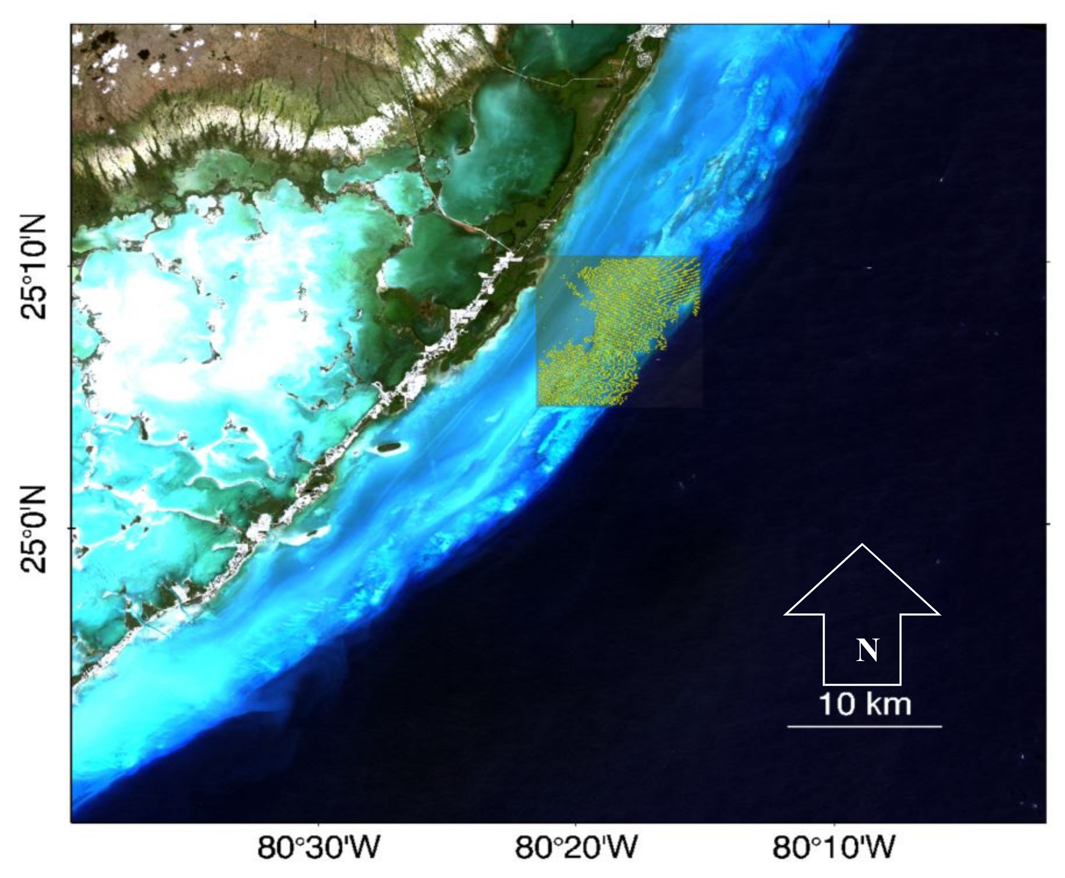
The Florida Keys is a series of islands that extend from the southern end of Florida, USA, to the south–southwest. Their nearshore shallow waters include coral reef tracts, patch reefs, bank reefs, seagrass meadows, and unvegetated hard and soft bottom. This site was chosen because of its relatively clear waters, the good knowledge of seabed features, and availability of LiDAR-derived depth data for validating SDB estimates of water depth. The benthic environment of the section of the Florida Keys used in this study is dominated by extensive seagrass beds, with some patches of reef and unconsolidated sediments. Figure 1 shows this area with the distribution of bathymetric LiDAR data used for validating the SDB estimates in this study.
2.2. Satellite Data
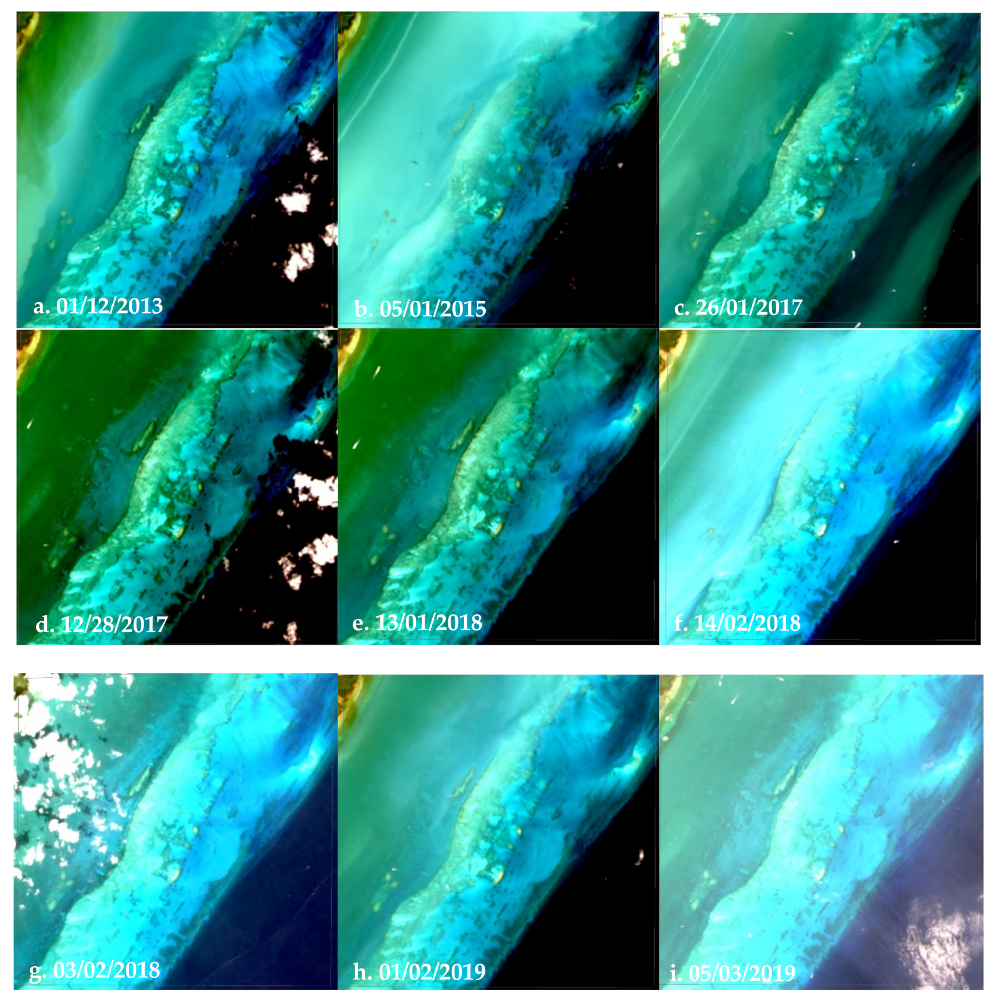
Nine L8 images (Figure 2) from the Florida Keys, acquired during both optimal and near-optimal conditions for SDB, were downloaded from the archive of the United States Geological Survey after visually inspecting all available images from May 2013 to May 2019. L8 OLI (Operational Land Imager) collects visible, Near Infrared (NIR) and Short-wave infrared (SWIR) spectral band imagery at 30 m spatial resolution. In addition to the improved positional accuracy of 14 m, compared to 50 m for its predecessors in the Landsat series, L8 includes coastal and aerosol (433–453 nm) and blue (450–515 nm) bands for coastal and bathymetric mapping [25,26].
2.3. LiDAR Data
To validate the SDB estimates, a bathymetry topographic digital elevation model (DEM) was acquired from the National Oceanic and Atmospheric Administration (NOAA) National Centres for Environment Information (NCEI) coastal LiDAR archive. The LiDAR data collection was conducted in December 2014 over South Florida and the Florida Keys as part of efforts by NOAA to study sea level rise and coastal flooding impacts on US coasts. Several LiDAR sources including topographic and bathymetric LiDAR sensors were used to develop and create a suite of tiled bathymetric–topographic DEMs for South Florida and the Florida Keys [27]. A portion of the DEM tiles covering the study site (Figure 1) was retrieved from the Office of Coastal Managements Data Access Viewer [28] where all DEM data are archived. The DEMs, with a vertical accuracy of approximately 0.5 m, are referenced vertically to the North American Vertical Datum of 1988. Horizontal positions were provided in geographic coordinates and referenced to the North American Datum of 1983 [29,30]. A portion of the collection covering the Florida Keys coastal area was referenced to mean sea level and resampled from 0.3 m to 30 m to match the spatial resolution of L8.
3. Methodology
3.1. Data Preprocessing
3.1.1. Atmospheric Correction
We implemented two types of AC methods for water depth retrieval: (1) we used ACOLITE to process L8 images into Rrs values (henceforth Rrsraw) and (2) then applied a correction factor to reduce errors in the original ACOLITE output and create new corrected Rrs values (henceforth Rrscorrected). ACOLITE [24], specifically designed for AC over water surfaces, is an AC method that estimates Lw by simulating contributions from molecular (Rayleigh) and particulate (aerosol) scattering using a 6SV-based LUT [31]. Based on Ruddick et al. [32], aerosol reflectance is estimated by determining a per-tile aerosol type (or epsilon) from the ratio of reflectances in two bands over water pixels where Lw can be assumed to be zero. Then, the epsilon is used to extrapolate the observed aerosol reflectance to the visible bands to remove atmospheric contributions. ACOLITE was originally designed for processing L8 images, but it has been modified and updated to also process Sentinel-2 data [33]. Furthermore, the most recent version, which can be adapted to commercial sensors such as Pleiades, contains an additional AC scheme (now the default setting) called the dark spectrum fitting (DSF) algorithm, as well as a sun glint correction scheme [34]. In this study, ACOLITE (version 20170113.0) was used to produce all Rrs images, which are the direct input into the bathymetry algorithm. The default SWIR option (1609 and 2201 nm band combination) was implemented for all images. This band combination takes advantage of the longest-wavelength SWIR band, where water absorption is the highest. In a previous study [23], in which a range of AC algorithms were compared and validated against in situ Lw from 14 AERONET-OC stations, statistically significant relationships were demonstrated between errors in ACOLITE’s Rrs estimates for L8′s 443 nm and 482 nm bands and three environmental variables: Solar Zenith Angle (SZA), Aerosol Optical Thickness (AOT) at 865 nm (AOT865), and wind speed (u10); probable but statistically non-significant relationships were also demonstrated for the 561 nm and 655 nm bands. Using multiple linear regression, we therefore derived a set of coefficients that were used to estimate the error of ACOLITE’s Rrs estimates for each of those four bands in each image, as a function of SZA, AOT865, and wind speed. Then, each of the four bands used for depth retrieval in this study was corrected using Equation (1):
where Rrscorrected and Rrsraw are the Rrs images with and without correction, respectively; and a, b, c, and d are coefficients obtained through fitting a linear model to the data from Ilori et al. [23]. SZA was obtained from the metadata of each L8 scene. AOT865 was processed and obtained using the l2gen processor in the SeaDAS software, and an average value used for each image was calculated by randomly sampling multiple pixels over the area of the study site. Wind speed data were obtained from the National Centers for Environmental Prediction Reanalysis project [35], where 6 h global wind speed estimates are archived. Table 1 presents the value of each environmental parameter for each image used in this study.
Rrscorrected = Rrsraw − (a + b*SZA + c*AOT865 + d*u10)
3.1.2. Sun Glint Correction
As sun glint correction is not inherently part of the ACOLITE version used in this study, we implemented the NIR method [36] to remove specular reflection off the sea surface for images where glint was visually obvious. This method assumes that for optically deep areas (where radiation reflected from the seafloor has a negligible influence on Lw), any remaining NIR signal after AC must be due to sea surface reflection. Thus, glint intensity and removal is performed by establishing a linear relationship between the NIR and visible bands over an optically deep area in the image, and that relationship is then used across all water pixels to reduce Rrs for the visible bands to its assumed glint-free value.
3.1.3. Estimation of Noise Equivalent Reflectance
Bathymetry model inversion based on least squares optimization techniques is generally sensitive to environmental noise [37,38]; thus, high environmental noise may make images unsuitable for bathymetry extraction. The noise-equivalent difference in reflectance, NE∆Rrs (sr−1), is a measure of image noise, with contributions from the sensor (e.g., instrument degradation) and the environment (e.g., variability in atmosphere and water surface state) [37,38]. The NE∆Rrs can be used to assess the suitability of a satellite imagery for aquatic remote sensing applications. For example, it has been used to determine the suitability of the Compact Airborne Spectrographic Imager (CASI) for benthic mapping [11]. Therefore, following AC, we estimated the NE∆Rrs (sr−1) [39] by calculating the band-wise standard deviation of Rrs from a 33 × 33-pixel window over a homogeneous optically deep area using Equation (2) [40]. This approach assumes that any observed spectral variations in the selected area is due to noise; thus, selected pixels must be as homogenous as possible for a robust standard deviation estimate. Ideally, the NE∆Rrs should be lower than 0.00025 sr−1 in each of the visible bands [41], which was the case for all nine images used in this study. Table 2 shows the per-band value obtained for each of the 9 images used in this study.
where Rrs is the standard deviation in each band over an as homogeneous as possible area of optically deep water within the image.
3.1.4. Parameterization of Environmental Properties
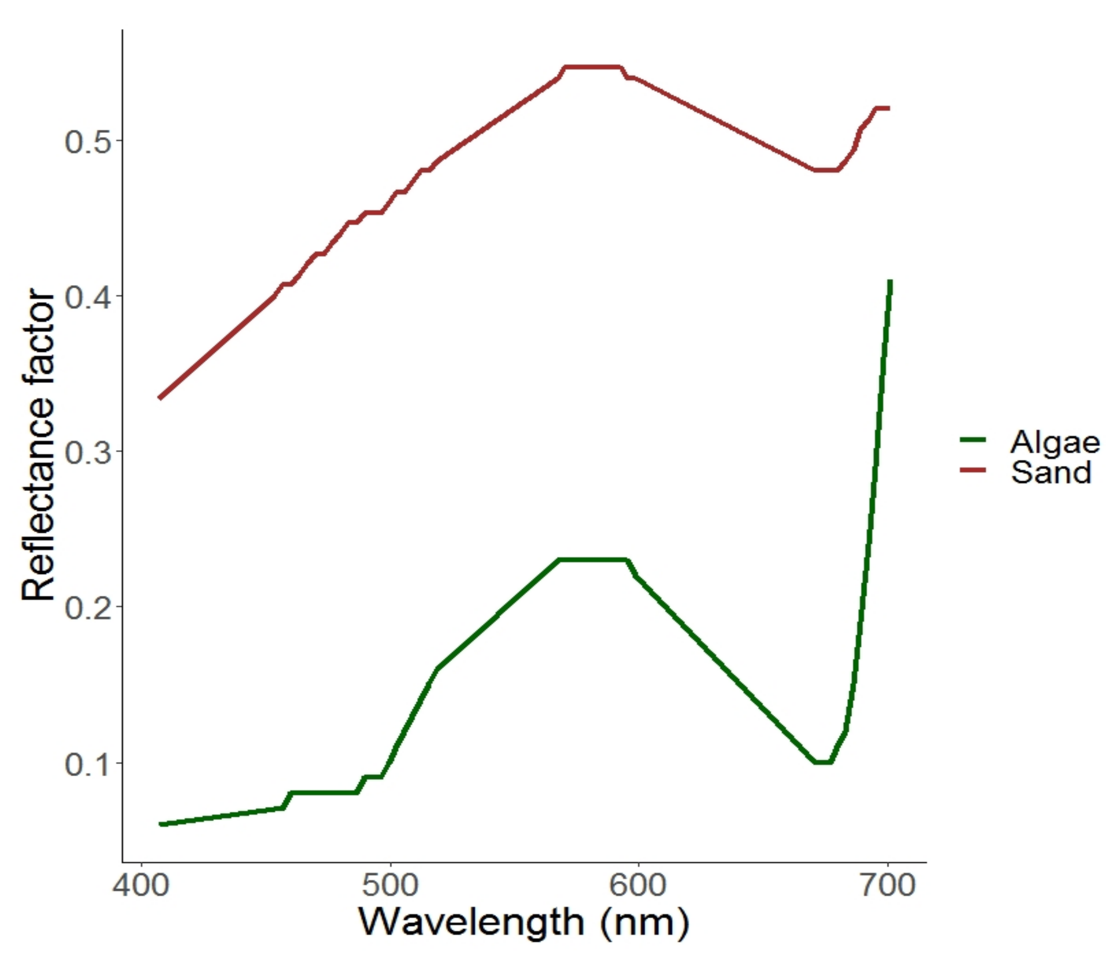
To implement the physics-based approach to SDB, values of optical properties and substratum spectral reflectance that are representative of the environment in question are needed. Water inherent optical properties (IOP) (P440, G440, and X550) parameterization for forward modeling for each site was based on assessment from Level 3 OC products from the Visible Infrared Imaging Radiometer Suite Visible Infrared Imaging Radiometer Suite (VIIRS) Generalized Inherent Optical Property (GIOP) algorithms [42]. P440 is the phytoplankton absorption coefficient at 440 nm, G440 is the absorption of gelbstoff and detrital materials coefficient at 440 nm, and X550 is the particulate backscattering of suspended particles coefficient at 550 nm. Using parameter values obtained from these OC products, ranges of values for each parameter were determined by observing the lowest and highest parameter values for all dates from GIOVANNI, which is an online visualization tool for OC products [43]. Then, values slightly lower and higher than the observed lowest and highest values, respectively, were chosen (Table 3). As part of the inversion model, seafloor reflectance spectra are also needed. We used two seafloor spectra (Figure 3), based on the area’s benthic description [44]. Depth (Z), which was also needed for forward modeling, was set to 0.1 and 25 m with the understanding that depth penetration greater than 25 m would be difficult.
3.1.5. Forward Modeling of Remote Sensing Reflectance
To derive water depth, we applied a modified version of the semi-analytical inversion model of Lee et al. [17,18] to the atmospherically corrected images. In this inversion scheme, the sub-surface remote sensing reflectance, rrs, (the ratio of upwelling radiance to downwelling irradiance just below the surface) is related to absorption (a) and backscattering properties () of the water column, the seafloor reflectance (ρ), and water depth (H). For nadir-viewing satellites, the model can be expressed as:
where rrs, the subsurface remote-sensing reflectance, is expressed as:
where and are the sub-surface solar zenith and sub-surface sensor viewing angles, respectively. Absorption (a) and backscattering coefficients () are functions of (1) the absorption coefficient of phytoplankton at 440 nm, P; (2) the absorption coefficient of colored dissolved materials at 440 nm, G; and (3) the backscattering coefficient of suspended particles at 550 nm, X. These are expressed as:
where and are the absorption and backscattering coefficients of pure water, respectively [45], is the specific absorption of coefficient of phytoplankton (normalized to a value of 1.0 at 440 nm), λ is the center wavelength, and Y is the spectral shape that depends on the particulate shape and size.
While Lee’s inversion model uses the albedo of only one key benthic substrate (sand), our model includes a parameterization to set the seafloor reflectance as a linear mix of the two bottom types (i.e., sand and algae; [46]). To forward model the Rrs as a function of water depth, water quality parameters, and the seafloor reflectance, the adaptive look-up table (ALUT) method [11,16] was implemented, which ensures efficient construction and search through the table. In this approach, an LUT consisting of the modeled Rrs values of L8 bands 1–4, seafloor reflectance (Figure 3), water optical properties (absorption and scattering characteristics of water), and water depths of the optically shallow zone of the area in question (Table 3) is constructed. With realistic minimum and maximum values of all environmental parameters in the table, the LUT construction is optimized by using a hierarchical structure to efficiently cover the range of expected Rrs values while minimizing the under- or over-sampling of spectrally similar regions of environmental space, which is common with discretization by regular intervals in conventional forward models. For example, a small change in depth in shallow water areas will cause a significant/large change in Rrs, and will typically result in under-sampling if the depth parameter is discretized by regular intervals. Likewise, oversampling may occur in deep water areas where a small change in Rrs is expected [11,16]. To identify the best parameter values to be included in the hierarchy in the ALUT technique, discretization is based on an evenly sampled spectral space and not on an evenly sampled parameter space (e.g., water depth). This approach requires bounded ranges for all the modeled parameters, for which we used the value ranges in Table 3.
3.1.6. Inversion of Remote Sensing Reflectance
Model inversion was subsequently performed using the binary space partitioning (BSP) approach [11,16], as described in Knudby et al. [12]. Briefly, this technique subdivides the LUT created during forward modeling into different nodes. First, the BSP splits the whole LUT into two (left and right child nodes) and subsequently subdivides the nodes into a partitioning tree, which facilitates the optimization of the per-pixel LUT search. After model inversion and depth retrieval, water depths were corrected for tidal height at the time of each image acquisition using tidal height estimates obtained from Oregon State University’s tide prediction service [47].
Depth cannot be accurately estimated for optically deep pixels (i.e., where reflection off the seafloor is a negligible component of the radiance measured by the sensor); thus, we estimated a depth threshold value for each scene to distinguish between optically deep and optically shallow areas. These threshold values were obtained by calculating the mean minus 2 standard deviations of depth predictions within a 33 × 33 window of homogeneous optically deep water. Results are reported for each scene both a) for the full depth range, and b) for depths from the surface and down to these scene-specific thresholds.
3.2. Validation of Depth Estimates
Validation of depth estimates from the two AC procedures was performed by comparing the estimated depths to the LiDAR data. The number of depth estimates used for validation (Table 4) varied between the nine images due to differences in the number of pixels for which depth was successfully estimated, as pixels that did not pass the AC’s internal quality checks (e.g., due to clouds), pixels with negative depths, and pixels that were visually impacted by boats, wake, or cloud shadows were eliminated prior to validation. Based on the remaining pixels, we used the coefficient of determination (R2), RMSE (root-mean-squared-error) (Equation (9)) and bias (Equation (10)) to compare the accuracy of the uncorrected and corrected SDB estimates with the LiDAR datasets. The RMSE is used to measure the accuracy of the estimated depth values; and bias is used to indicate overestimation (positive value) or underestimation (negative value):
where n is the number of observations, and xest and xobs are the estimated and measured depths, respectively. Values closer to zero for both error metrics indicate a better result. SDB obtained with Rrsraw and Rrscorrected are hereafter referred to as SDBraw and SDBcorrected, respectively. These summary statistics (R2, RMSE, and bias) were calculated both for the full depth range and for depths ranging from the surface down to the per-scene depth threshold (Table 4).
4. Result and Discussion
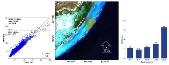
Scatterplots showing water depth estimates produced from both Rrsraw and Rrscorrected images and the LiDAR depth measurements are shown in Figure 4, and summary statistics (R2, RMSE, and bias) are listed in Table 4.
The RMSE values for SDBraw/SDBcorrected estimates range from 1.35/1.05 m to 2.21/2.04 m for the full depth range, and from 1.21/0.95 m to 2.19/1.89 m when applying the per-scene depth threshold. These values are broadly comparable with other SDB studies (e.g., [10,13,14,41,48]). For example, Dekker et al. [48], who compared one empirical and five physics-based approaches to bathymetry mapping using hyperspectral imagery, reported RMSE values between 0.86 (best) and 4.71 m (worst) for depths less than 13 m for two clear tropical waters in the Bahamas and eastern Australia, suggesting that our results are typical of what should be expected from a physics-based bathymetry method. It is worth mentioning here that impacts from recent hurricanes over parts of the Florida Keys, notably in 2016 and 2017, have resulted in an average increase of approximately +0.3 m in seafloor elevation over different habitat types [49,50]. Such changes were not accounted for in this study and may have had a small effect on the results, although it is worth noting that the best SDB estimate is from 2019 [Figure 4h], after the hurricanes.
Figure 4 shows that accuracy decreases with depth for both SDBraw and SDBcorrected, particularly beyond approximately 15 m where the proportion of the measured signal originating from reflection at the seafloor becomes very small. In general, for depths shallower than 15 m, SDBcorrected points cluster more tightly around the 1:1 line that do the SDBraw points.
4.1. Effects of Image Conditions on Depth Accuracy
4.1.1. Turbidity
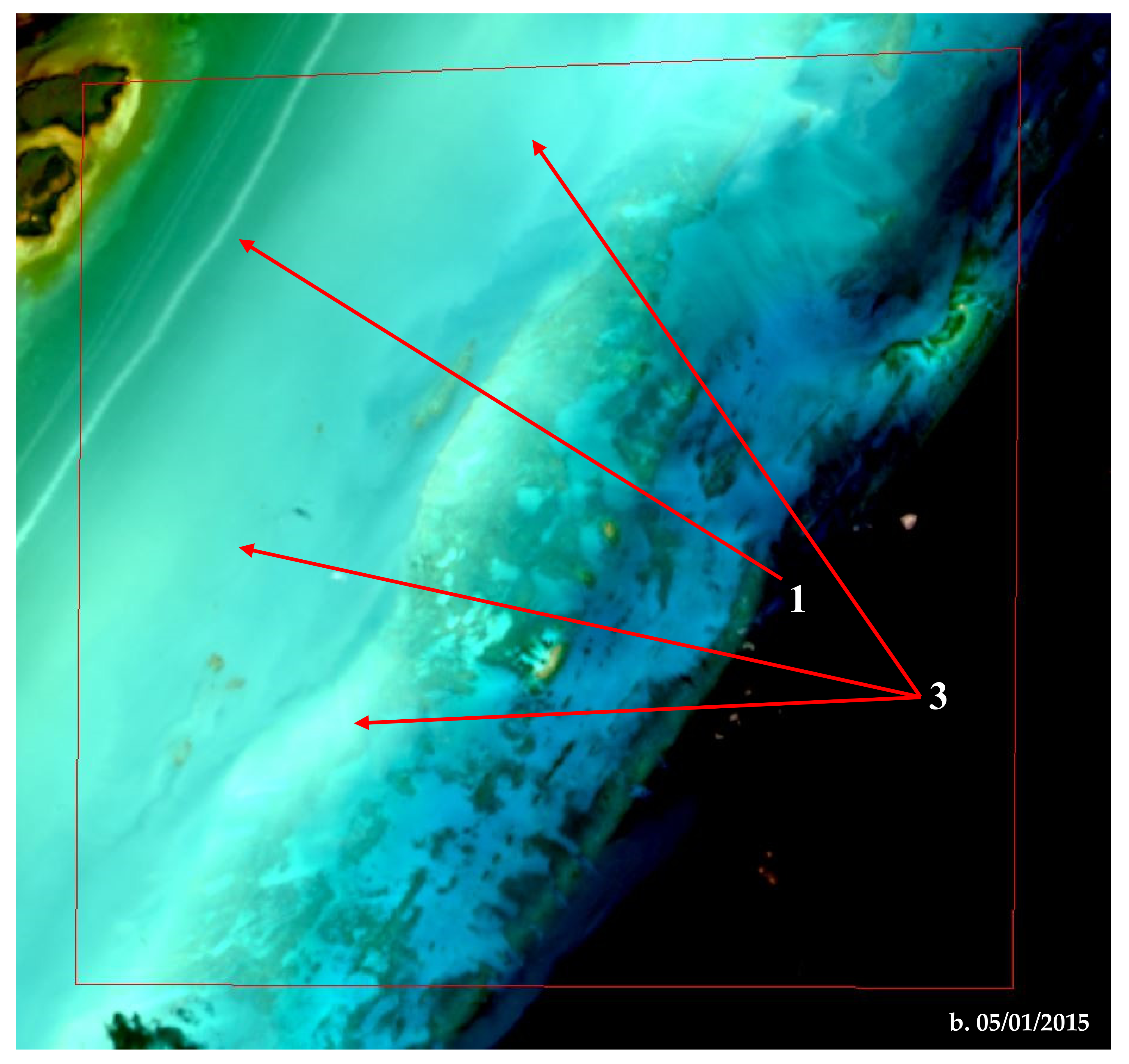
Out of the nine Rrs images we applied the correction factor to, eight corrections resulted in negative RMSE changes when considering the two depth limits used in this study, with reductions ranging from 0.09 to 0.48 m (for the full depth range) and 0.07 to 0.46 m (for the per-scene depth threshold). For both depth limits, only one correction resulted in increased RMSE (i.e., the image from 01/05/2015, see Table 4) (RMSE values for SDBraw and SDBcorrected will hereafter be referred to as RMSEraw and RMSEcorrected, respectively). For this image, accurate depth estimates were not possible beyond approximately 14 m (Figure 4b), regardless of correction, and RMSEcorrected increased marginally by 0.01 m for the full depth range and by 0.04 m for the per-scene depth threshold (i.e., 0–11.23 m). A visual inspection of this image shows sediment plumes in the study area (Figure 5b), which suggests that turbidity contributed to an underestimation of water depth for both SDBraw and SDBcorrected [14], and the image is of marginal use for SDB, regardless of correction. Similarly, one of the two corrected images with the lowest RMSE reduction for the full depth range also has what looks to be a silt plume emerging from nearshore channels in the southwestern portion of the area for which depth was calculated (Figure 5a). For this image, RMSE value marginally decreased by 0.09 m for the full depth range and by 0.26 m for the per-scene depth threshold (i.e., 1 to 12.03 m).
4.1.2. Glint
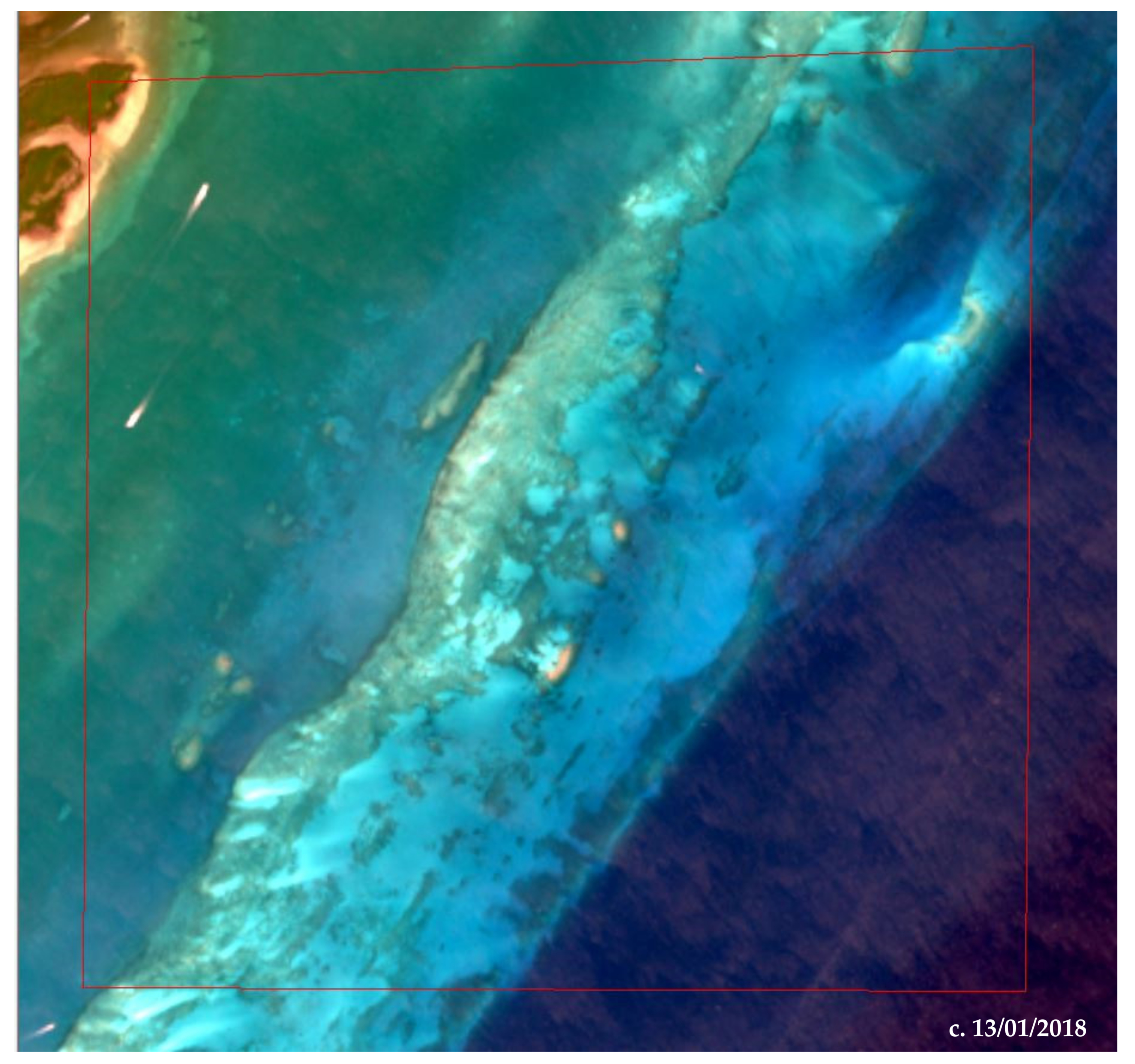
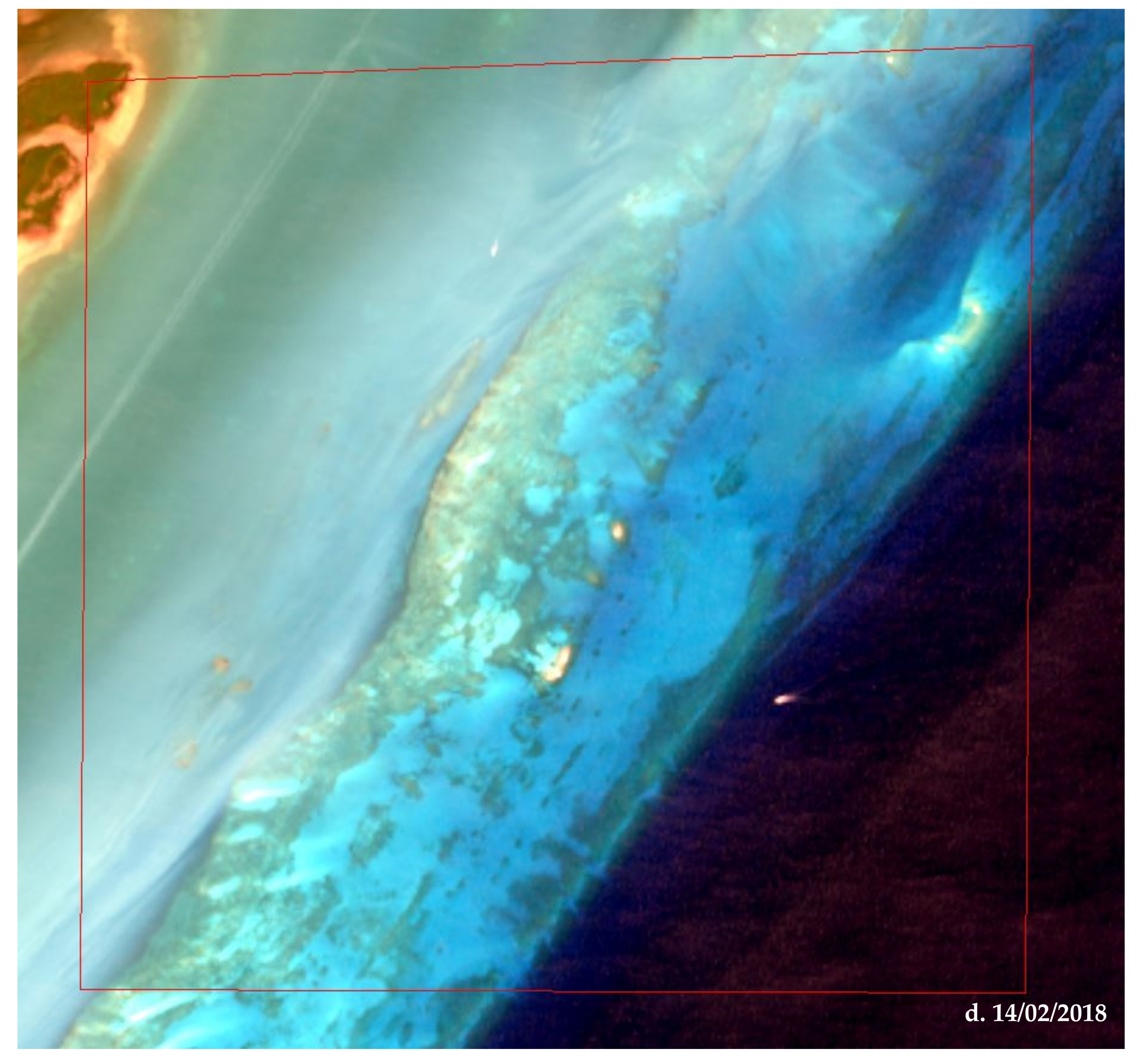
With RMSEraw values of 2.21 m and 2.19 m for the full depth range and the per-scene depth threshold, respectively, the image from 13/01/2018 produces the poorest SDBraw and SDBcorrected estimates out of the nine images. As shown in Table 4, this image has the highest RMSE and positive bias values. A visual inspection of this image (Figure 5c) indicates the presence of a moderate glint. Glint correction was not performed, as the image did not show any noticeable improvement after the initial testing. Likewise, for the image from 14/02/2018 (Figure 5d), the high negative bias values for both depth ranges, regardless of correction (Table 4), may be attributed to residual sun glint in addition to light turbidity. While an attempt was made to de-glint this image as described in Section 3.1.2, given that the NIR-based de-glinting method [36] implemented (1) relies on manual selection of deep-water pixels to estimate glint contribution, (2) assumes that there are glint-free pixels among those selected [51], and (3) assumes a homogenously low Rrs(NIR) across all water pixels, failure to meet these conditions may have resulted in the observed residual glint. For example, Rrs(NIR) may be non-negligible in glint-free but very shallow or turbid waters, or where reflective vegetation such as seagrass is close to the upper water column [52]. For these two images, the correction produces slightly reduced RMSE values (Figure 4e,f), substantially so for their respective depth thresholds (Table 4).
4.2. Effect of Wind Speed and SZA on SDB Performance
Out of the eight scenes whose SDB performance improved with the correction for the Rrs images, greater corrections were done for five scenes (i.e., Figure 4a,c–f) acquired with SZA > 49° (Table 1), and one scene (i.e., Figure 4g) acquired during high wind speed (3.21 m/s) (Table 1), when considering the per-scene depth thresholds. Likewise, when considering the full depth range, greater corrections were also done for the same number of scenes under similar environmental conditions, with the exception of the image from 26 January 2017, whose change in RMSE is −0.09 m (Table 4). It should be noted that the most noticeable RMSE reduction for SDBcorrected images for both depth limits considered in this study (i.e., Figure 4d) was observed for the scene with the highest SZA and highest wind speed. This is supporting evidence for the existence of a relationship between ACOLITE’s overestimation of Rrs in the first two bands of L8 and these two environmental variables [23], and it gives an idea of the magnitude of its impact on SDB performance. A recent study [53] also found a dependency between AC retrieval accuracy and wind speed in coastal waters. While there is strong evidence to conclude that the correction factor used in this study lowers RMSE values for images with high wind speed, it should be noted that wind speed data used in this study come from 6-h estimates in reanalysis model, and thus, they have their own uncertainty. For this reason, more testing may be needed for a firmer conclusion about the relationship between ACOLITE’s error and wind speed.
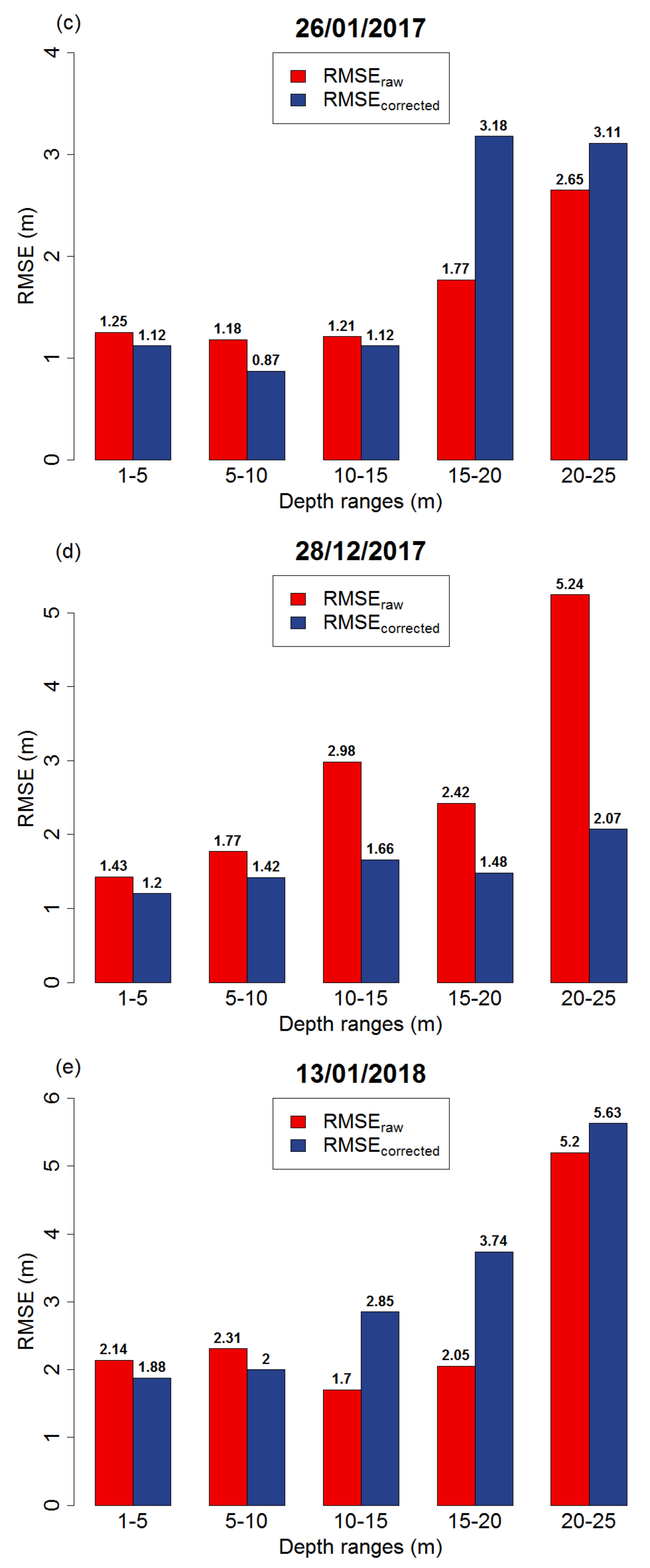
4.3. Bathymetry Estimates at Different Depth Ranges
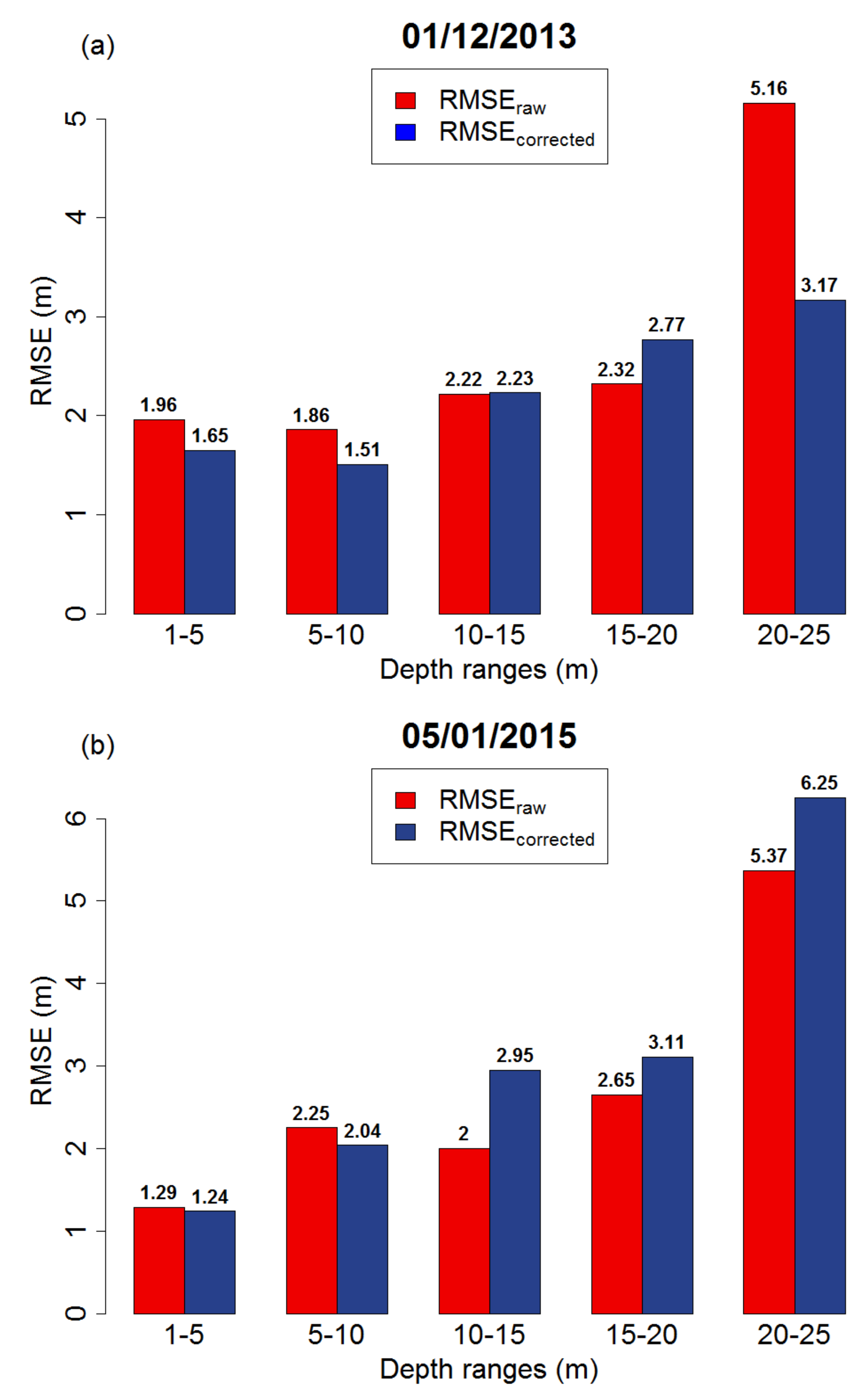
Figure 6 shows the performance of SDBraw and SDBcorrected for each image, binned to 5 m depth increments for the 1–25 m depth range. The accuracy of SDB estimates decreases with increasing depth for both SDBraw and SDBcorrected. While higher RMSE values should be expected at deeper depths due to the diminishing signal from seafloor reflectance, it should be noted that the number of LiDAR points for validation is also smaller at deeper depths, leading to increased uncertainty around the RMSE values reported at these depths.
4.4. SDB Estimates Using an Ensemble Approach
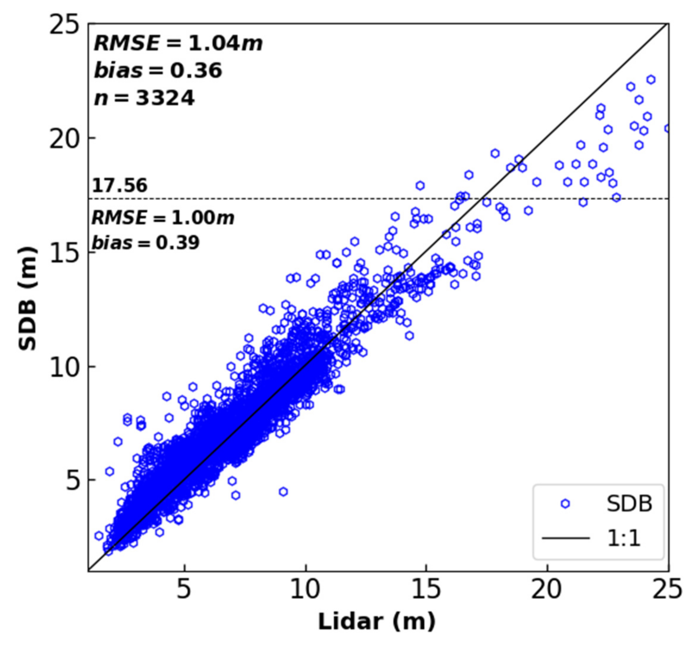
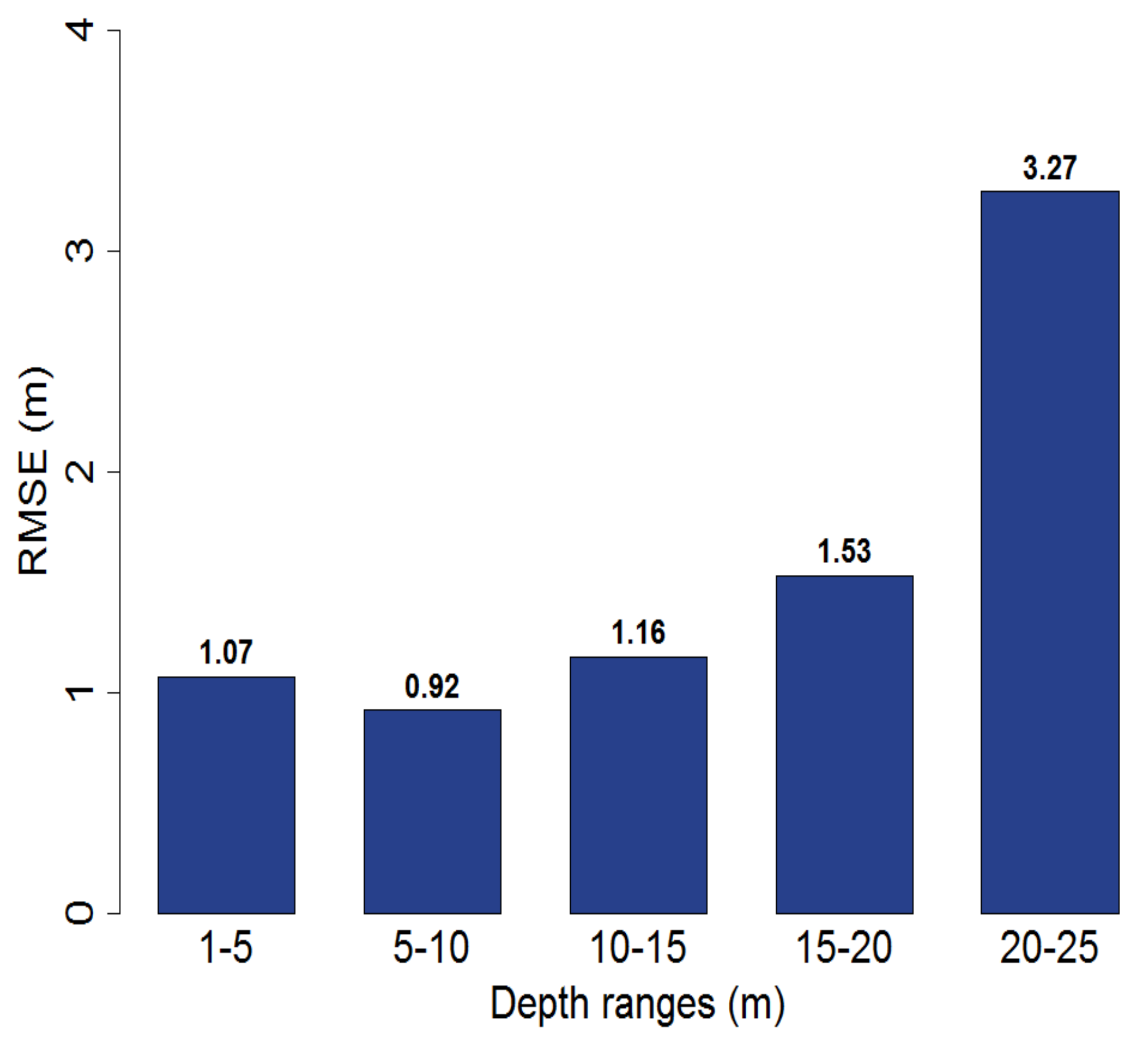
Most SDB studies are based on a single image for each study area, with researchers typically selecting the best available image using visual inspection [14]. Our results indicate that this may not be a robust approach. To illustrate the problem, we invite readers to visually inspect the nine images used in this study (Figure 2) and identify the one that looks most suitable for SDB. Then, proceed to Table 4 to see if it was indeed the one that produced the best results, as measured by RMSE, bias, or R2. An informal test among our colleagues, all of whom work on OC remote sensing, suggests that it is not easy to identify the best scene. However, a unique advantage of optical remote sensing is the repetitive acquisition of images over the same area. This is especially important for SDB, where the suitability of a given image is determined by transient environmental factors, such as cloud and aerosols, sea surface state, and turbidity [54]. We explored one way of taking advantage of the multiple images available for the study area by testing an ensemble approach in which we calculated the per-pixel median depth value of all nine corrected images (i.e., SDBcorrected) used in this study. Then, we compared the resulting depth estimates with those obtained using the best individual image from the analysis in Section 4.1 (i.e., the image from 01/02/2019, see Table 4). Figure 7 shows that the results produced by the ensemble are very similar to those obtained with the best individual image. SDB estimates up to approximately 15 m are similar to the SDBcorrected estimates from the 01/02/2019 image, as are the RMSE values for the 1–5, 5–10, and 10–15 m depth ranges (Figure 8). Outliers are noticeably reduced in the ensemble result when compared to any of the sub-optimal images that were also included in its calculation, suggesting that the use of median depth is effective in eliminating noise in the ensemble. Thus, the ensemble approach eliminates the need for the selection of a single best image, while producing SDB results of similar accuracy. In this context, it is noteworthy that one of the two best images (i.e., image from 05/03/2019) is also the one with the lowest NE∆Rrs in bands 1, 2, and 4, as well as the second-lowest NE∆Rrs in band 3 (Table 2). This suggests that one effective way to pre-screen images, either for a single best image approach or to determine which images should be included in an ensemble, could be to estimate NE∆Rrs and select those images with the lowest values across the visible bands.
5. Conclusions
In this study, we demonstrated the use of Landsat 8 data for physics-based SDB in US coastal waters. A state-of-the-art AC method (ACOLITE) was used to convert per-pixel radiometric units to Rrs, and an RTM was inverted to estimate water depth, which was compared to airborne LiDAR validation data. The results showed that ACOLITE can be used to produce SDB from imagery that is free of conditions such as clouds, glint, sediments plumes, boats and wakes, with an accuracy (RMSE 1.34 m for 1–25 m depth range and 1.21 m for approximately 1–15 m depth range) comparable to that reported from empirical and physics-based SDB elsewhere. To account for ACOLITE’s known overestimation of Rrs for Landsat 8′s coastal and blue bands, we applied a correction factor, which was calculated as a function of solar zenith angle, aerosol optical thickness, and wind speed, to obtain a corrected set of Rrs images. This correction further improved bathymetry estimates for eight of the nine scenes we tested, with the resulting changes in bathymetry RMSE ranging from +0.01 m (worse) to −0.48 m (better) for a 1 to 25 m depth range, and from + 0.04 m (worse) to −0.46 m (better) for an approximately 1–16 m depth range. Using a total of nine Landsat 8 images, we showed that the correction factor improved SDB results, both on average (ΔRMSE = −0.22 m) and for the best single image (ΔRMSE = −0.30 m) for the 1–25 m depth range. SDB improvements from application of the correction factor were the greatest for images acquired at a high solar zenith angle and at high wind speeds, where ACOLITE is known to have the greatest bias. The correction method demonstrated in this study can be implemented with any appropriate AC algorithm. Finally, we demonstrated that an ensemble approach based on multiple images, with acquisitions ranging from optimal to sub-optimal conditions, can be used to derive bathymetry with a result that is similar to what can be obtained from the best individual image. This is important because it is rarely visually obvious which of several images is best for SDB, and the ensemble approach can be automated to reduce time spent on pre-screening and filtering scenes, and it can potentially also reduce the amount of missing pixels caused by clouds and cloud shadows encountered in any single image. Automating SDB will ultimately facilitate the efficient and operational use of the globally available L8 (and other multispectral) datasets.
Author Contributions
Conceptualization, C.O.I. and A.K.; Methodology, C.O.I. and A.K.; Software, C.O.I. and A.K.; Validation, C.O.I. and A.K.; Formal Analysis, C.O.I.; Resources, C.O.I. and A.K.; Writing—Original Draft Preparation, C.O.I.; Writing—Review & Editing, C.O.I. and A.K.; Supervision, A.K. All authors have read and agreed to the published version of the manuscript.
Funding
This research received no external funding.
Acknowledgments
The authors wish to thank the United States Geological Survey (USGS) for the distribution of Landsat 8 Level-1 data products. We are deeply thankful to Quinten Vanhellemont and Kevin Ruddick for the development of ACOLITE and the NASA Ocean Biology Processing Group for the development of the SeaDAS software. We also thank Chris Roelfsema and his team for making the spectra data used in this study publicly available online.
Conflicts of Interest
The authors declare no conflict of interest.
References
- Ramnath, V.; Feygels, V.; Kalluri, H.; Smith, B. CZMIL (Coastal Zone Mapping and Imaging Lidar) Bathymetric Performance in Diverse Littoral Zones. In Proceedings of the OCEANS 2015 OCEANS MTS/IEEE, Washington, DC, USA, 19–22 October 2015. [Google Scholar]
- Parker, H.; Sinclair, M. The Successful Application of Airborne LiDAR Bathymetry Surveys Using Latest Technology. In Proceedings of the 2012 Oceans—Yeosu, Yeosu, Korea, 21–24 May 2012. [Google Scholar]
- Tonina, D.; McKean, J.A.; Benjankar, R.M.; Wright, C.W.; Goode, J.R.; Chen, Q.; Reeder, W.J.; Carmichael, R.A.; Edmondson, M.R. Mapping river bathymetries: Evaluating topobathymetric LiDAR survey. Earth Surf. Process. Landf. 2019, 44, 507–520. [Google Scholar] [CrossRef]
- Wozencraft, J.M.; Lillycrop, W.J. SHOALS Airborne Coastal Mapping: Past, Present, and Future. J. Coast. Res. 2003, 38, 207–215. [Google Scholar]
- Gao, J. Bathymetric mapping by means of remote sensing: Methods, accuracy and limitations. Prog. Phys. Geogr. 2009. [Google Scholar] [CrossRef]
- Su, H.; Liu, H.; Heyman, W. Automated derivation of bathymetric information from multi-spectral satellite imagery using a non-linear inversion model. Mar. Geodesy 2008, 31, 281–298. [Google Scholar] [CrossRef]
- Lyzenga, D.R. Passive remote sensing techniques for mapping water depth and bottom features. Appl. Opt. 1978, 17, 379–383. [Google Scholar] [CrossRef] [PubMed]
- Lyzenga, D.R. Remote sensing of bottom reflectance and water attenuation parameters in shallow water using aircraft and landsat data. Int. J. Remote Sens. 1981, 2, 71–82. [Google Scholar] [CrossRef]
- Lyzenga, D.R. Shallow-water bathymetry using combined Lidar and passive multispectral scanner data. Int. J. Remote Sens. 1985, 6, 115–125. [Google Scholar] [CrossRef]
- Chénier, R.; Faucher, M.A.; Ahola, R. Satellite-derived bathymetry for improving Canadian Hydrographic Service charts. ISPRS Int. J. Geo Inf. 2018, 7, 306. [Google Scholar] [CrossRef] [Green Version]
- Hedley, J.; Roelfsema, C.; Koetz, B.; Phinn, S. Capability of the Sentinel 2 mission for tropical coral reef mapping and coral bleaching detection. Remote Sens. Environ. 2012, 120, 145–155. [Google Scholar] [CrossRef]
- Knudby, A.; Ahmad, S.K.; Ilori, C. The Potential for Landsat-Based Bathymetry in Canada. Can. J. Remote Sens. 2016, 42, 367–378. [Google Scholar] [CrossRef]
- Olayinka, I.; Knudby, A. Satellite-Derived Bathymetry Using a Radiative Transfer-Based Method: A Comparison of Different Atmospheric Correction Methods. In Proceedings of the OCEANS 2019 MTS/IEEE SEATTLE, Seattle, DC, USA, 27–31 October 2019. [Google Scholar] [CrossRef]
- Casal, G.; Hedley, J.D.; Monteys, X.; Harris, P.; Cahalane, C.; McCarthy, T. Satellite-derived bathymetry in optically complex waters using a model inversion approach and Sentinel-2 data. Estuar. Coast. Shelf Sci. 2020, 241, 106814. [Google Scholar] [CrossRef]
- Mobley, C.D.; Sundman, L.K.; Davis, C.O.; Bowles, J.H.; Downes, T.V.; Leathers, R.A.; Montes, M.J.; Bissett, W.P.; Kohler, D.D.R.; Reid, R.P.; et al. Interpretation of hyperspectral remote-sensing imagery by spectrum matching and look-up tables. Appl. Opt. 2005, 44, 3576. [Google Scholar] [CrossRef] [PubMed]
- Hedley, J.; Roelfsema, C.; Phinn, S.R. Efficient radiative transfer model inversion for remote sensing applications. Remote Sens. Environ. 2009, 113, 2527–2532. [Google Scholar] [CrossRef]
- Lee, Z.; Carder, K.L.; Mobley, C.D.; Steward, R.G.; Patch, J.S. Hyperspectral remote sensing for shallow waters I. A semianalytical model. Appl. Opt. 1998, 37, 6329–6338. [Google Scholar] [CrossRef] [PubMed]
- Lee, Z.; Carder, K.L.; Mobley, C.D.; Steward, R.G.; Patch, J.S. Hyperspectral remote sensing for shallow waters: 2. Deriving bottom depths and water properties by optimization. Appl. Opt. 1999, 38, 3831–3843. [Google Scholar] [CrossRef] [PubMed] [Green Version]
- Pahlevan, N.; Schott, J.R.; Franz, B.A.; Zibordi, G.; Markham, B.; Bailey, S.; Schaaf, C.B.; Ondrusek, M.; Greb, S.; Strait, C.M. Landsat 8 remote sensing reflectance (Rrs) products: Evaluations, intercomparisons, and enhancements. Remote Sens. Environ. 2017, 190, 289–301. [Google Scholar] [CrossRef]
- Doxani, G.; Vermote, E.; Roger, J.C.; Gascon, F.; Adriaensen, S.; Frantz, D.; Hagolle, O.; Hollstein, A.; Kirches, G.; Li, F.; et al. Atmospheric correction inter-comparison exercise. Remote Sens. 2018, 10, 352. [Google Scholar] [CrossRef] [Green Version]
- Warren, M.A.; Simis, S.G.H.; Martinez-Vicente, V.; Poser, K.; Bresciani, M.; Alikas, K.; Spyrakos, E.; Giardino, C.; Ansper, A. Assessment of atmospheric correction algorithms for the Sentinel-2A MultiSpectral Imager over coastal and inland waters. Remote Sens. Environ. 2019, 225, 267–289. [Google Scholar] [CrossRef]
- Zhang, M.; Hu, C. Evaluation of Remote Sensing Reflectance Derived from the Sentinel-2 Multispectral Instrument Observations Using POLYMER Atmospheric Correction. IEEE Trans. Geosci. Remote Sens. 2020, 58, 1–8. [Google Scholar] [CrossRef]
- Ilori, C.O.; Pahlevan, N.; Knudby, A. Analyzing performances of different atmospheric correction techniques for Landsat 8: Application for coastal remote sensing. Remote Sens. 2019, 11, 469. [Google Scholar] [CrossRef] [Green Version]
- Vanhellemont, Q.; Ruddick, K. Advantages of high quality SWIR bands for ocean colour processing: Examples from Landsat-8. Remote Sens. Environ. 2015, 161, 89–106. [Google Scholar] [CrossRef] [Green Version]
- Storey, J.; Choate, M.; Lee, K. Landsat 8 operational land imager on-orbit geometric calibration and performance. Remote Sens. 2014, 6, 11127–11152. [Google Scholar] [CrossRef] [Green Version]
- Czapla-Myers, J.; McCorkel, J.; Anderson, N.; Thome, K.; Biggar, S.; Helder, D.; Aaron, D.; Leigh, L.; Mishra, N. The ground-based absolute radiometric calibration of Landsat 8 OLI. Remote Sens. 2015, 6, 11127–11152. [Google Scholar] [CrossRef] [Green Version]
- Sutherland, M.G.; Amante, C.J.; Carignan, K.S.; Lancaster, M.N.; Love, M.R. NOAA National Centers for Environmental Information Topo-Bathymetric Digital Elevation Modeling: Florida Keys and South Florida. 2016. Available online: https://www.ngdc.noaa.gov/mgg/dat/dems/tiled_tr/florida_keys_tiled_navd88_2016.pdf (accessed on 25 July 2020).
- NOAA. Data Access Viewer. Available online: https://coast.noaa.gov/dataviewer/#/lidar/search/ (accessed on 13 May 2020).
- Cooperative Institute for Research in Environmental Sciences. Continuously Updated Digital Elevation Model (CUDEM)—1/9 Arc-Second Resolution Bathymetric-Topographic Tiles. NOAA National Centers for Environmental Information, 2015. Available online: https://doi.org/10.25921/ds9v-ky35 (accessed on 13 March 2020).
- National Centers of Environmental Information; NESDIS; NOAA; U.S. Department of Commerce. U.S. Coastal Lidar Elevation Data—Including the Great Lakes and Territories, 1996—Present. 2015. Available online: https://catalog.data.gov/harvest/object/abccfcac-9d89-475f-b0f3-58db5d317a86/html (accessed on 25 July 2020).
- Kotchenova, S.Y.; Vermote, E.F.; Levy, R.; Lyapustin, A. Radiative transfer codes for atmospheric correction and aerosol retrieval: Intercomparison study. Appl. Opt. 2008, 47, 2215–2226. [Google Scholar] [CrossRef] [PubMed] [Green Version]
- Ruddick, K.G.; Ovidio, F.; Rijkeboer, M. Atmospheric correction of SeaWiFS imagery for turbid coastal and inland waters. Appl. Opt. 2000, 39, 897–912. [Google Scholar] [CrossRef] [PubMed] [Green Version]
- Vanhellemont, Q.; Ruddick, K. Acolite for Sentinel-2: Aquatic Applications of MSI Imagery. In Proceedings of the 2016 ESA Living Planet Symposium, Prague, Czech Republic, 9–13 May 2016. [Google Scholar]
- Vanhellemont, Q.; Ruddick, K. Atmospheric correction of metre-scale optical satellite data for inland and coastal water applications. Remote Sens. Environ. 2018, 216, 586–597. [Google Scholar] [CrossRef]
- Kalnay, E.; Kanamitsu, M.; Kistler, R.; Collins, W.; Deaven, D.; Gandin, L.; Iredell, M.; Saha, S.; White, G.; Woollen, J.; et al. The NCEP/NCAR 40-Year Reanalysis Project. Bull. Am. Meteorol. Soc. 1996, 77, 437–472. [Google Scholar] [CrossRef] [Green Version]
- Hedley, J.D.; Harborne, A.R.; Mumby, P.J. Simple and robust removal of sun glint for mapping shallow-water benthos. Int. J. Remote Sens. 2005, 26, 2107–2112. [Google Scholar] [CrossRef]
- Botha, E.J.; Brando, V.E.; Dekker, A.G. Effects of per-pixel variability on uncertainties in bathymetric retrievals from high-resolution satellite images. Remote Sens. 2016, 131, 459. [Google Scholar] [CrossRef] [Green Version]
- Jay, S.; Guillaume, M.; Minghelli, A.; Deville, Y.; Chami, M.; Lafrance, B.; Serfaty, V. Hyperspectral remote sensing of shallow waters: Considering environmental noise and bottom intra-class variability for modeling and inversion of water reflectance. Remote Sens. Environ. 2017, 200, 352–367. [Google Scholar] [CrossRef]
- Brando, V.E.; Dekker, A.G. Satellite hyperspectral remote sensing for estimating estuarine and coastal water quality. IEEE Trans. Geosci. Remote Sens. 2003, 41, 1378–1387. [Google Scholar] [CrossRef]
- Wettle, M.; Brando, V.E.; Dekker, A.G. A methodology for retrieval of environmental noise equivalent spectra applied to four Hyperion scenes of the same tropical coral reef. Remote Sens. Environ. 2004, 93, 188–197. [Google Scholar] [CrossRef]
- Brando, V.E.; Anstee, J.M.; Wettle, M.; Dekker, A.G.; Phinn, S.R.; Roelfsema, C. A physics based retrieval and quality assessment of bathymetry from suboptimal hyperspectral data. Remote Sens. Environ. 2009, 113, 755–770. [Google Scholar] [CrossRef]
- Maritorena, S.; Siegel, D.A.; Peterson, A.R. Optimization of a semianalytical ocean color model for global-scale applications. Appl. Opt. 2002, 41, 2705–2714. [Google Scholar] [CrossRef] [PubMed]
- Acker, J.G.; Leptoukh, G. Online analysis enhances use of NASA Earth Science Data. Trans. Am. Geophys. 2007, 88, 14–24. [Google Scholar] [CrossRef]
- NCCOS. Benthic Habitat Mapping of Florida Coral Reef Ecosystems to Support Reef Conservation and Management. 2014. Available online: https://coastalscience.noaa.gov/project/benthic-habitat-mapping-florida-coral-reef-ecosystems/ (accessed on 22 March 2019).
- Pope, R.M.; Fry, E.S. Absorption spectrum (380–700 nm) of pure water II Integrating cavity measurements. Appl. Opt. 1997, 36, 8710–8723. [Google Scholar] [CrossRef]
- Roelfsema, C.; Phinn, S. Spectral Reflectance Library of Selected Biotic and Abiotic Coral Reef Features in Heron Reef, Bremerhaven, PANGAEA. 2006. Available online: https://epic.awi.de/id/eprint/31865/ (accessed on 1 August 2020).
- Egbert, G.D.; Erofeeva, S.Y. Efficient inverse modeling of barotropic ocean tides. J. Atmos. Oceanic Technol. 2002, 19, 183–204. [Google Scholar] [CrossRef] [Green Version]
- Dekker, A.G.; Phinn, S.R.; Anstee, J.; Bissett, P.; Brando, V.E.; Casey, B.; Fearns, P.; Hedley, J.; Klonowski, W.; Lee, Z.P.; et al. Intercomparison of shallow water bathymetry, hydro-optics, and benthos mapping techniques in Australian and Caribbean coastal environments. Limnol. Oceanogr. Methods 2011, 9, 396–425. [Google Scholar] [CrossRef] [Green Version]
- Yates, K.Y.; Zawada, D.G.; Arsenault, S.R. Seafloor Elevation Change from 2016 to 2017 at Looe Key, Florida Keys—Impacts from Hurricane Irma: U.S. Geological Survey Data Release. 2019. Available online: https://catalog.data.gov/dataset/seafloor-elevation-change-from-2016-to-2017-at-looe-key-florida-keys-impacts-from-hurricane-irm (accessed on 22 July 2020).
- Yates, K.Y.; Zawada, D.G.; Arsenault, S.R. Seafloor Elevation Change from 2016 to 2017 at Crocker Reef, Florida Keys—Impacts from Hurricane Irma. 2019. Available online: https://coastal.er.usgs.gov/data-release/doi-P9JI465S/ (accessed on 27 July 2020).
- Harmel, T.; Chami, M.; Tormos, T.; Reynaud, N.; Danis, P.A. Sunglint correction of the Multi-Spectral Instrument (MSI)-SENTINEL-2 imagery over inland and sea waters from SWIR bands. Remote Sens. Environ. 2018, 204, 308–321. [Google Scholar] [CrossRef]
- Overstreet, B.T.; Legleiter, C.J. Removing sun glint from optical remote sensing images of shallow rivers. Earth Surf. Process. Landf. 2017, 42, 318–333. [Google Scholar] [CrossRef]
- Estrella, E.H.; Grotsch, P.; Gilerson, A.; Malinowski, M.; Ahmed, S. Blue band reflectance uncertainties in coastal waters and their impact on retrieval algorithms. In Proceedings of the SPIE 11420, Ocean Sensing and Monitoring XII, Vancouver, BC, Canada, 27 April–1 May 2020. [Google Scholar] [CrossRef]
- Jégat, V.; Pe, S.; Freire, R.; Klemm, A.; Nyberg, J. Satellite-Derived Bathymetry: Performance and Production. In Proceedings of the Canadian Hydrographic Conference, Halifax, NS, Canada, 16–19 May 2016. [Google Scholar]
Figure 1.
Landsat 8 image showing the upper Florida Keys. Bathymetric LiDAR data used for validation are shown in yellow.
Figure 1.
Landsat 8 image showing the upper Florida Keys. Bathymetric LiDAR data used for validation are shown in yellow.

Figure 2.
(a–i) A section of Florida Keys image showing the RGB composite of each image used in this study.
Figure 2.
(a–i) A section of Florida Keys image showing the RGB composite of each image used in this study.

Figure 3.
Spectral reflectance of the seafloor used in this study.

Figure 4.
(a–i) Scatterplots of satellite-derived bathymetry estimates versus LiDAR measurements. Red points show water depth estimates obtained from original ACOLITE outputs; blue points show estimates obtained after applying the correction factor. The 1:1 line is shown in black. The dotted horizontal lines and values above them denote threshold values beyond which the water column is deemed optically deep. Threshold value was calculated using Mean − 2 Standard deviation of a 33 × 33 window pixel selected over an optically deep homogeneous area in an image.

Figure 5.
(a–d) Maps showing different confounding factors that might have affected SDB estimates from some images. 1: Boat-generated wake. 2: Plume emerging from a near river discharge. 3: Moving boats. Sun glint can be observed in Figure 5c,d as visible texture around the southeastern part of the images.


Figure 6.
(a–i) RMSE values obtained for SDBraw and SDBcorrected estimates at different water depths. Results at higher depth (>15 m) should be interpreted with caution, as the number of depth observations for those depth ranges was comparably lower than those available for shallower depth ranges. Depth observation for each depth range is as follows: 1–5 m: approximately 900 points, 5–10 m: approximately 1800 points, 10–15 m: approximately 300 points, 15–20 m: approximately 40 points, and 20–25 m: approximately 20 points. Note that the y-axes have different ranges for each date to facilitate comparison between RMSEraw and RMSEcorrected for each single scene.


Figure 7.
Scatterplots of ensemble-based satellite-derived bathymetry estimates vs. LiDAR measurements. Blue dots show estimates obtained after applying a correction to the Rrs images. The solid line represents the 1:1 relationship. The dotted line shows the per-scene depth threshold value and its statistical metrics.

Figure 8.
RMSE values obtained for the ensemble-based SDB estimates at different water depths.


Table 1.
Environmental parameter variables for each image. AOT865: Aerosol Optical Thickness (AOT) at 865 nm, SZA: Solar Zenith Angle.
Table 1.
Environmental parameter variables for each image. AOT865: Aerosol Optical Thickness (AOT) at 865 nm, SZA: Solar Zenith Angle.
| Scene Date (dd/mm/yyyy) | SZA (Degrees) | AOT865 | u10 (m/s) |
|---|---|---|---|
| 01/12/2013 | 50.36 | 0.081 | 5.29 |
| 05/01/2015 | 52.79 | 0.088 | 1.07 |
| 26/01/2017 | 50.13 | 0.083 | 2.49 |
| 28/12/2017 | 52.98 | 0.076 | 6.45 |
| 13/01/2018 | 52.14 | 0.142 | 3.11 |
| 14/02/2018 | 45.63 | 0.12 | 4.84 |
| 02/03/2018 | 40.66 | 0.11 | 3.21 |
| 01/02/2019 | 49.02 | 0.122 | 3.74 |
| 05/03/2019 | 39.74 | 0.143 | 4.67 |
Table 2.
The noise equivalent difference in reflectance (NE∆Rrs), computed from a kernel of 33 × 33 pixels from an optically deep and homogeneous area, for each image used in this study.
Table 2.
The noise equivalent difference in reflectance (NE∆Rrs), computed from a kernel of 33 × 33 pixels from an optically deep and homogeneous area, for each image used in this study.
| Scene Dates (dd/mm/yyyy) | Band 1 | Band 2 | Band 3 | Band 4 |
|---|---|---|---|---|
| 01/12/2013 | 0.000200 | 0.000154 | 0.000096 | 0.000061 |
| 05/01/2015 | 0.000136 | 0.000108 | 0.000084 | 0.000063 |
| 26/01/2017 | 0.000092 | 0.000072 | 0.000057 | 0.000042 |
| 28/12/2017 | 0.000151 | 0.000105 | 0.000081 | 0.000053 |
| 13/01/2018 | 0.000111 | 0.000103 | 0.000069 | 0.000047 |
| 14/02/2018 | 0.000157 | 0.000129 | 0.000108 | 0.000063 |
| 02/03/2018 | 0.000126 | 0.000110 | 0.000069 | 0.000043 |
| 01/02/2019 | 0.000148 | 0.000127 | 0.000100 | 0.000063 |
| 05/03/2019 | 0.000086 | 0.000081 | 0.000059 | 0.000042 |
Table 3.
Parameter ranges used for forward modeling.
| P | G | X | Z |
|---|---|---|---|
| 0.006–0.04 | 0.004–0.04 | 0.0005–0.006 | 0.1–25 |
Table 4.
Summary validation statistics for satellite-derived bathymetry (SDB) estimates (SDBraw and SDBcorrected) for the two depth limits in this study. Bold letters in the root-mean-squared-error (RMSE) column indicate where an observed difference between SDBraw and SDBcorrected estimates is more than 0.1 m.
| Scene Date dd/mm/yyyy | Max Depth (m) | RMSE (m) (SBDraw/SBDcorrected) | Bias (SBDraw/SBDcorrected) | R2 (SBDraw/SBDcorrected) | Number of Validation Points |
|---|---|---|---|---|---|
| 01/12/2013 | 25 | 1.96/1.66 | 0.83/0.84 | 0.66/0.79 | 3102 |
| 13.80 | 1.80/1.50 | 0.85/0.73 | 0.58/0.71 | 2988 | |
| 05/01/2015 | 25 | 2.02/2.03 | −0.17/−0.46 | 0.71/0.71 | 3317 |
| 11.23 | 1.84/1.88 | −0.46/−0.71 | 0.53/0.53 | 3050 | |
| 26/01/2017 | 25 | 1.34/1.25 | 0.49/0.09 | 0.85/0.85 | 3311 |
| 12.03 | 1.21/0.95 | 0.57/0.23 | 0.81/0.85 | 3142 | |
| 28/12/2017 | 25 | 1.87/1.39 | 1.16/0.41 | 0.74/0.81 | 3148 |
| 17.54 | 1.85/1.39 | 1.18/0.42 | 0.79/0.81 | 3086 | |
| 13/01/2018 | 25 | 2.21/2.04 | 1.45/1.40 | 0.66/0.76 | 2804 |
| 15.21 | 2.19/1.89 | 1.48/1.35 | 0.56/0.74 | 2721 | |
| 14/02/2018 | 25 | 1.86/1.72 | −1.15/−1.04 | 0.77/0.79 | 3316 |
| 14.81 | 1.80/1.69 | −1.12/−1.01 | 0.71/0.74 | 3247 | |
| 02/03/2018 | 25 | 2.03/1.65 | 0.71/0.68 | 0.61/0.74 | 3268 |
| 16.84 | 1.98/1.62 | 0.69/0.67 | 0.53/0.71 | 3226 | |
| 01/02/2019 | 25 | 1.35/1.05 | 0.55/0.62 | 0.83/0.92 | 3255 |
| 14.61 | 1.33/1.02 | 0.54/0.64 | 0.76/0.90 | 3187 | |
| 05/03/2019 | 25 | 1.36/1.27 | 0.76/0.53 | 0.89/0.89 | 3312 |
| 16.39 | 1.32/1.25 | 0.79/0.55 | 0.85/0.83 | 3263 |
© 2020 by the authors. Licensee MDPI, Basel, Switzerland. This article is an open access article distributed under the terms and conditions of the Creative Commons Attribution (CC BY) license (http://creativecommons.org/licenses/by/4.0/).
Share and Cite
MDPI and ACS Style
Ilori, C.O.; Knudby, A. An Approach to Minimize Atmospheric Correction Error and Improve Physics-Based Satellite-Derived Bathymetry in a Coastal Environment. Remote Sens. 2020, 12, 2752. https://doi.org/10.3390/rs12172752
AMA Style
Ilori CO, Knudby A. An Approach to Minimize Atmospheric Correction Error and Improve Physics-Based Satellite-Derived Bathymetry in a Coastal Environment. Remote Sensing. 2020; 12(17):2752. https://doi.org/10.3390/rs12172752
Chicago/Turabian StyleIlori, Christopher O., and Anders Knudby. 2020. "An Approach to Minimize Atmospheric Correction Error and Improve Physics-Based Satellite-Derived Bathymetry in a Coastal Environment" Remote Sensing 12, no. 17: 2752. https://doi.org/10.3390/rs12172752
Note that from the first issue of 2016, this journal uses article numbers instead of page numbers. See further details here.