Article

Particle Size Parameters of Particulate Matter Suspended in Coastal Waters and Their Use as Indicators of Typhoon Influence

1
Key Laboratory of Marine Geology and Environment, Institute of Oceanology, Chinese Academy of Sciences, Qingdao 266071, China
2
Laboratory for Marine Geology, Qingdao National Laboratory for Marine Science and Technology, Qingdao 266061, China
3
Center for Ocean Mega-Science, Chinese Academy of Sciences, Qingdao 266071, China
4
College of Earth and Planetary Sciences, University of Chinese Academy of Sciences, Beijing 100049, China
5
School of Forestry, Northeast Forestry University, Harbin 150040, China
*
Author to whom correspondence should be addressed.
Remote Sens. 2020, 12(16), 2581; https://doi.org/10.3390/rs12162581
Submission received: 1 July 2020 / Revised: 27 July 2020 / Accepted: 8 August 2020 / Published: 11 August 2020

Abstract

:
The power law particle size distribution (PSD) slope parameter is commonly used to characterize sediment fluxes, resuspension, aggregates, and settling rates in coastal and estuarine waters. However, particle size distribution metrics are also very useful for understanding sediment source and dynamic processes. In this study, a method was proposed to employ the particle size parameters commonly used in sedimentary geology (average particle size (ø), sorting, skewness, and kurtosis) as indicators of changes in sediment dynamic processes, and MODIS images were used to estimate these parameters. The particle size parameters were estimated using a Mie scattering model, Quasi-Analytical Algorithm (QAA) analysis algorithm, and least squares QR decomposition (LSQR) solution method based on the relationship between the power law distribution of the suspended particles and their optical scattering properties. The estimates were verified by field measurements in the Yellow Sea and Bohai Sea regions of China. This method provided good estimates of the average particle size (ø), sorting, and kurtosis. A greater number of wavebands (39) was associated with more accurate particle size distribution curves. Furthermore, the method was used to monitor changes in suspended particulate matter in the vicinity of the Heini Bay of China before and after the passage of a strong storm in August 2011. The particle size parameters represented the influence of a strong typhoon on the distribution of the near-shore sediment and, together with the PSD slope, comprehensively reflected the changes in the near-shore suspended particulate matter. This method not only established the relationship between remote sensing monitoring and the historical sediment record, it also extends the power law model to the application of sediment source and dynamic processes in coastal waters.

Graphical Abstract

1. Introduction

Particle size distribution (PSD) is a fundamental property of natural water particle assemblages and plays an important indicative role in many fields of marine science [1]. Particle size affects physical transport and biochemical interactions in seawater [2]. Understanding the relative proportions of small and large particles at the ocean surface is critical for understanding marine ecology and biogeochemistry. The theoretical relationship between the backscattering spectral slope and the power law PSD slope has been used to derive the seawater surface PSD (hereinafter referred to as the surface PSD) from ocean color remote sensing images on a global scale. These estimates have been applied to identify phytoplankton functional groups and to estimate carbon sequestration within the ocean [2,3]; however, these generally straightforward approaches cannot accommodate the optical complexity of coastal regions that have waters rich in terrigenous material [4,5].
Coastal areas are characterized by a large range of physical, biochemical, and optical properties due to the presence of river inputs, freshwater, land, and anthropogenic impacts. This means that the ocean optical properties in these areas may be different from those of the plankton-dominated ocean waters [6,7]. In coastal marine environments, mineral particles tend to account for a large proportion of suspended particulate matter due to river discharge, coastal erosion caused by waves and currents, and seafloor resuspension [8]. In the open ocean, the abundance of mineral particles is typically low. There is still no consensus that scattering particles in even the most oligotrophic seas may be organic or inorganic [9], and current estimation models attribute the optical properties of the surface water to plankton microorganisms and detrital matter [10]. As a result, these models do not work well in coastal areas. The influences of extreme weather or human activities render the power law PSD slope unable to adequately describe the complexity of coastal waters; that is, a simple approximation cannot fully capture the complexity of sediment re-suspension and transport under the influence of strong ocean dynamics [11,12].
Geologists often categorize extreme weather events by interpreting the sudden coarsening and sorting of sediment particles in geological sedimentary sequences as a result of episodic floods and storm events [13,14,15,16]. Many sedimentology studies support the principle that sediment properties can be used as a proxy for reconstructing sedimentary environments [17,18,19,20]. Sediment particle size is a basic physical property of sediments and its distribution varies with sediment transport and sediment hydrodynamic characteristics [21]. The sediment particle size parameters (average particle size, median particle size, sorting, skewness, kurtosis, standard deviation, etc.) are often used to classify sedimentary environments [22,23,24]. The particle size distribution curve can directly determine the migration pattern of each particle size group [25,26] and can be used to characterize environmental and climatic changes. Unfortunately, collecting on-site measurement data during extreme weather events is logistically and technically difficult. Additionally, differences in the trajectory, intensity, and velocity of each storm current across the continental shelf have different effects on the deposition and suspension of particulate matter. Therefore, it is very difficult to generalize the sedimentary characteristics of extreme weather at the coastal continental shelf. Remote sensing technologies, which provide monitoring over a wide spatial coverage with high temporal resolution, are expected to be important for addressing the sediment particle size distribution problem.
Considering the effects of near-shore mineral particles on scattering and the limitations of the power law PSD slope, numerous studies have attempted to quantify the PSD and its changes by focusing on parameters, such as the median particle size, or other non-parametric descriptions [27,28,29,30], such as the particle beam attenuation index or the backscattering attenuation index [31], average particle size [5], the proportion of sand, silt, and clay [32]. Some studies have calculated the distribution of the PSD angle scattering model [33]. Although these parameters can better describe the distribution characteristics of the regional particle size, they remain inadequate indicators of the complex coastal environment.
In this study, the relationship between the backscattering coefficient and the particle size parameters (including the average particle size, sorting, skewness, kurtosis, and standard deviation) was established based on the PSD power law model. The particle size distribution curves and parameters describing the suspended sediment in surface seawater were estimated based on remote sensing reflectance data. Furthermore, a change in the parameters of surface suspended particulate matter was estimated by combining field measurements and MODIS images in the vicinity of the Heini Bay of China before and after the passage of a strong storm in August 2011. The particle size distribution curve and its parameters were compared with those in the sedimentary records to obtain indices that could characterize the impact of the ocean dynamic environmental on the particle size distribution.

2. Materials and Methods

2.1. Theory Background

Light scattering by a single particle depends on its particle size parameters (volume, diameter, surface area, etc.) [34] and on its refractive index relative to that of the surrounding medium (seawater). Mie scattering theory can be used to calculate the inherent optical properties of a known individual particle suspension, assuming that the suspension comprises non-interacting homogeneous spherical particles [28]. The optical properties of such a suspension follow a Junge-type power law. Mie theory can quantify the relationship between the particulate backscattering spectrum and the Junge PSD by providing efficiency factors for scattering ( Q b b ) [3]. The corresponding coefficient at the given wavelength is then obtained by integration over all particles of a given size [35]:
b b p ( λ ) = D m i n D m a x π 4 D 2 Q b b ( D , λ , m ) N 0 ( D D 0 ) ξ d D ,
where N 0 ( D D 0 ) ξ = N ( D )   is the number of particles per volume of seawater normalized by the size bin width (units of m–4), D is the particle diameter (m), D0 is a reference diameter, N0 is the particle differential number concentration at D0 (units of m–4), and ξ is the Junge slope of the PSD. The Junge slope, ξ, and the reference abundance, N0, are the two parameters of the Junge-type size distribution. The backscattering efficiency of an individual particle, Q b b ( D , λ , m ) , is a function of the wavelength of light in vacuo, λ, the diameter of the particle, D, and the particle’s complex index of refraction relative to the medium, m = n + n i , where the real part, n, is the ratio of the speed of light in seawater relative to that in the particle, and the imaginary part, n , is proportional to the particle material’s bulk absorption coefficient [36,37].
The number of particles per unit volume within each size class ( N ( D ) ) was computed by dividing the volume percentage content V ( D ) by the diameter (D) of a volume-equivalent sphere corresponding to the midpoint of each individual class [38,39]:
N ( D ) = 6 V ( D ) ( π D 3 ) 1

2.2. Calculations Approach

2.2.1. Particulate Backscattering Coefficient

In coastal areas, the optical properties of seawater components depend considerably on suspended and dissolved materials that do not covary with phytoplankton pigment concentration and are referred to as case 2 waters [40]. The total backscattering coefficients of a water body (   b b ( λ ) )   are the sum of the relevant bulk optical properties associated with each of the various components of a water body [41,42]:
b b ( λ ) = b b w ( λ ) + b b c ( λ ) + b b p ( λ ) ,
where b b ( λ ) , b b w ( λ ) , b b c ( λ ) , and   b b p ( λ ) are the backscattering coefficients of total, pure water, planktonic component, and suspended particles, respectively. According to Morel (1974) [43], the spectral variations of the scattering coefficient of pure water ( b w ) follow a ( λ ) 4.3 law:
b b w ( λ ) = 0.5 b w ( 500 ) ( λ 500 ) 4.3 .
Here, b b w ( λ ) can be obtained using the experimental results of Smith and Baker (1981) [44] and Morel et al. (2007) [45]. The experimental and theoretical results show that absorption and scattering by phytoplankton vary in a complementary manner. Thus, the phytoplankton backscattering coefficient can be obtained from the chlorophyll concentration and backscattering wavelength dependence using the method of Sathyendranath and Morel (1989) [41]:
b b c ( λ ) = 0.005 b c ( 550 ) ( a c ( 550 ) a c ( λ ) ) ,
where scattering by phytoplankton at 550 nm is estimated from the chlorophyll concentration (C, mg m–3), b c ( 550 ) = 0.12 C 0.63 , and a c ( λ ) is the absorption coefficient of chlorophyll. The total backscattering coefficient b b ( λ ) and the total absorption coefficient of chlorophyll a c ( λ ) used in the formula were obtained using the QAA_V5 algorithm. The algorithm description and parameter setting procedures are described in detail in Lee et al. (2002) [46] and Qing et al. (2011) [47].

2.2.2. Backscattering Efficiency

The backscattering efficiency ( Q b b ( D , λ , m ) ) was computed using the Bohren and Huffman (1983) [48] Mie code, based on the Mie scattering theory developed for homogenous spherical particles (usually called Mie scattering). In the Mie scattering calculation, the relative size is a dimensionless number that compares the spherical particle diameter (D) to the incident light wavelength ( λ ); that is, 2 π D / λ . The real part (n) of the refractive index (m) was computed as the integration of the percentage of each mineral with the corresponding refractive indices given by Kerr (1977) [30,49]. For the imaginary part n’ (λ) of the refractive index, the measured absorption coefficients of a suspended particle a b x ( λ ) [42,47] were calculated to assess the best n’ (λ) parameterization.

2.2.3. Particle Size Parameters Calculation
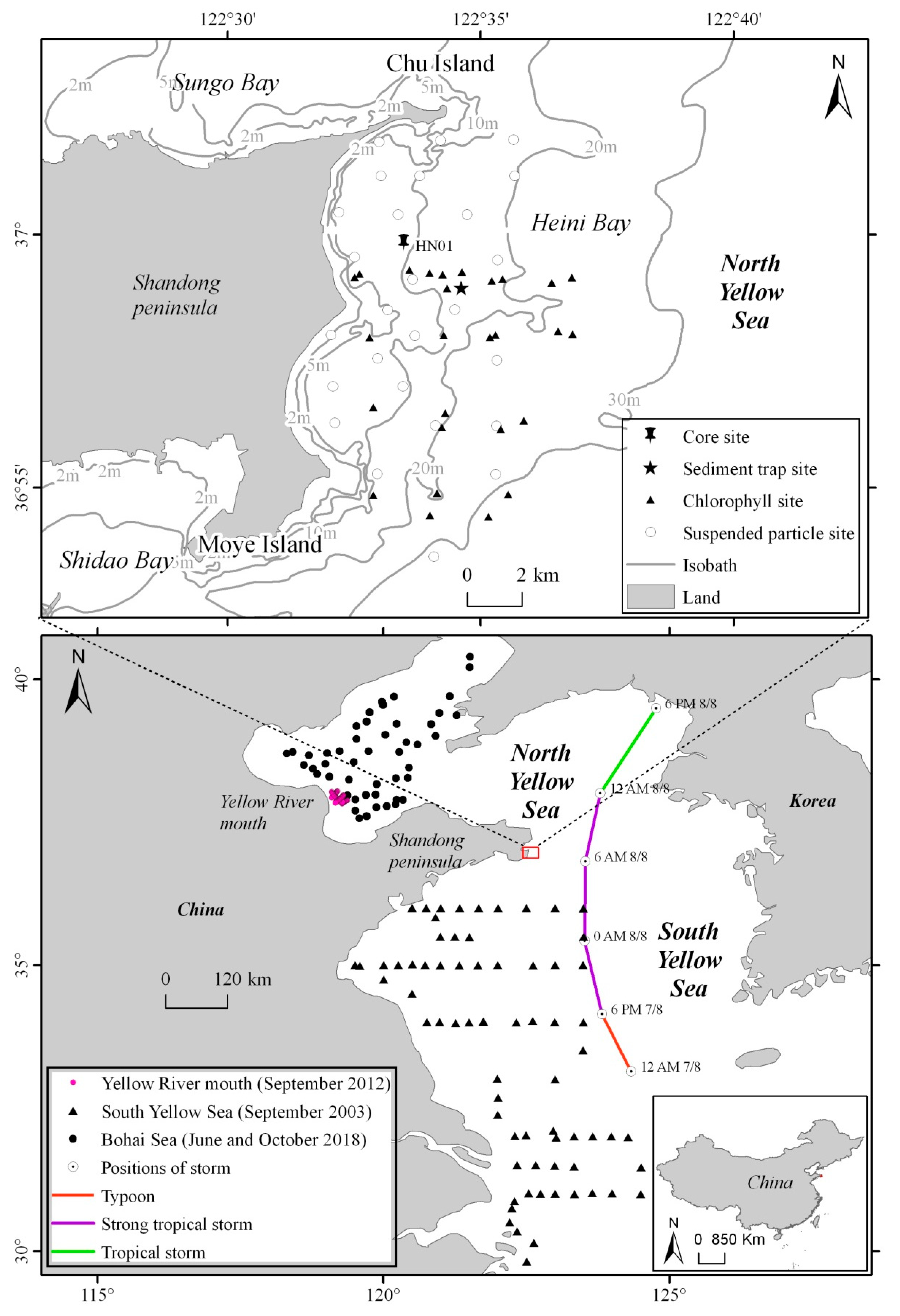
The experimental results obtained using a laser particle size analyzer represent the cumulative percentage f ( D ) of particles smaller than a certain particle size ( D ) . The relationship between those results and the volume percentage content V ( D ) of a certain particle size ( D ) is as follows:
V ( D ) = f ( D ) i + 1 f ( D ) i / log ( D i / D i 1 ) D m i n D m a x ( f ( D ) i + 1 f ( D ) i / log ( D i / D i 1 ) ) × 10 4 .
The volume concentration of a continuous size spectrum with n size classes has a physical constraint, i = 1 n V ( D i ) = 1 ,   0 V ( D i ) 1 . A formula for calculating the average particle size ( D ¯ ) of suspended particles is as follows:
D ¯ = i = 1 n ( V ( D i ) × D i ) .
According to a logarithmic scale method proposed by Krumbein (1934) [50], the formula for calculating the value of the average particle size (ø) is:
D ( ø ) ¯ = i = 1 n ( V ( D i ) × ( log 2 D i ) ) .
The sorting ( σ ) of suspended particles is used as a parameter for judging the particle size distribution range relative to the average particle size. The evaluation is based on the fact that similarly sized particles are often dynamically screened to a common pool, and the sorting process tends to be good. The formula describing the sorting process is:
σ = i = 1 n ( ( ( log 2 D i ) ( V ( D i ) × ( log 2 D i ) ) ) 2 × V ( D i ) ) .
The skewness ( S k ) indicates the symmetry of the grain size distribution curve, in which the particulate particle size is coarse, as indicated by the positive skewness grain size distribution curve (Table 1). The skewness is calculated according to:
S k = ( i = 1 n ( ( ( ( log 2 D i ) ( V ( D i ) × ( log 2 D i ) ) ) 3 × V ( D i ) ) ) / σ 3 .
The kurtosis ( K G ) is used to measure the degree to which the extreme value of the frequency distribution curve deviates from the extreme value of the normal distribution. A platykurtic distribution is one in which most of the values share about the same frequency of occurrence. A leptokurtic distribution has a higher frequency of particles within the peak range (Table 1). The kurtosis is calculated according to:
K G = ( i = 1 n ( ( ( ( log 2 D i ) ( V ( D i ) × ( log 2 D i ) ) ) 4 × V ( D i ) ) ) / σ 4 .
To solve Equation (1) numerically, substitution of Equations (2) and (6) into Equation (1) yields the further derivative Equation (12):
b b p ( λ j ) = 3 2 × i = 1 n Q b b ( D i , λ j , m j ) D i × V ( D i ) × d D i         ( j = 1 , 2 , , S ) ,
where n denotes the number of subintervals that divide the particle size range ( D m i n , D m a x ) . Therefore, Equation (1) can be described in terms of the discrete subintervals as:
B = A · V ,
A = a 1 , 1 a 1 , N a 2 , 1           a j , i         a s , 1 a S , N
B = [ b 1 ,       , b j ,       , b S ] T ,
V = [ V ( D 1 ) ,       ,   V ( D i ) ,       , V ( D N ) ] T ,
where A denotes the coefficient matrix, a j , i = 3 2 × Q b b ( D i , λ j , m j ) D i , B denotes the backscattering coefficient matrix, b j = b b p ( λ j ) , and S denotes the number of measurement wavelengths.
For this first type of Fredholm integral equation, the least squares QR decomposition (LSQR) algorithm can be used to solve it [32,51,52]. LSQR is one of the iterative regularization methods based on Lanczos bidiagonalization and QR factorization and first put forward by Paige and Saunders [53] in 1982 to solve the discrete optimization problems. The solution step is to first convert the arbitrary coefficient matrix into a square matrix, and then solve the least square solution of equations based on the bidiagonalization procedure Golub and Kahan (1965) [54].

2.3. Study Area

The above algorithm was verified over a small inner-shelf embayment at the easternmost tip of the Shandong Peninsula of China facing the Yellow Sea (Figure 1). This bay, Heini Bay, is a relatively independent sedimentary cell with a single material source primarily from coastal erosion and offshore suspended particles. The wave climate in this area features tide-dominated intermediate wave energy. The current velocity during winter is 80% of that during summer. The Yellow Sea littoral current flows through the nearshore area from N to S [55]. Sorting of the sediment was generally less than 1.4 (poorly sorted), transitioning from less than 0.6 (well sorted) in the nearshore area to 1.2 (poorly sorted) (Table 1) offshore [56]. The sorting distribution ran nearly parallel to the coast. The seabed sediments of the bay mostly consisted of muddy silt at water depths of less than 20 m, or coarse sand and gravel for water depths of 20–30 m, from the northern headland southward [57]. In recent decades, sediment refinement has occurred in the bay, and the outer sea clayey silt has gradually diffused into the bay, possibly because of nearby coastal aquaculture activities [56,58,59].
This area suffers an annual average of 1.6 tropical cyclones (30% of which land on the coast) [60,61,62]. On the morning of 8 August 2011, typhoon Muifa passed the eastern shore of the Shandong Peninsula approximately 100 km east of the study area with a maximum wind speed of 15.1 m s−1 and a significant wave height (Hs) of 5.8 m (Figure 1). Strong hydrodynamics induced approximately 9 times the settling particulate matter flux at a depth of 14 m compared to the value observed under normal weather conditions. An analysis of the sediment particulates indicated a high content of silt and clay with very little organic matter, and the particle size distribution changed from very poorly sorted to poorly sorted, from very positive skewness to positive skewness, and from very leptokurtic kurtosis to extremely leptokurtic kurtosis [62,63].

2.4. Sampling

During the passage of the typhoon Muifa, a time-series sediment trap (PARFLUX Mark78H-21, McLane Corporation, East Falmouth, MA, USA) was placed on a subsurface mooring at a depth of 14 m from 5 to 26 August 2011 (Figure 1). Nineteen settling particulate matter samples were collected every 24 h from 5 to 23 August 2011 (the samples from 24 to 26 August 2011 were contaminated and could not be used). To determine the sediment characteristics from historical sedimentary records, a short sediment core (HN01) sample, collected in June 2006, was analyzed. Details of the data collection and analysis methodology can be found in Liu et al. (2015) [62] and Liu et al. (2016; 2019) [56,63].
26 samples of suspended particulate matter were collected from a surface water depth of within 0.5 m between 13 and 21 November 2004, or between 28 April and 7 May 2006. The surface chlorophyll concentration and its corresponding spectral reflectance data were collected before the passage of the typhoon on 8 August 2011 (Figure 1).
The model relationship was verified by collecting surface suspended sediment particle size distribution data and surface spectral reflectance data measured during five sampling trips at the Yellow River mouth on 19–27 June 2004 and September 2012 (51 stations), the South Yellow Sea on 19 March–23 April 2003, and Bohai Sea in June 2018 and in September 2018 (Figure 1).

2.5. Sample Processing
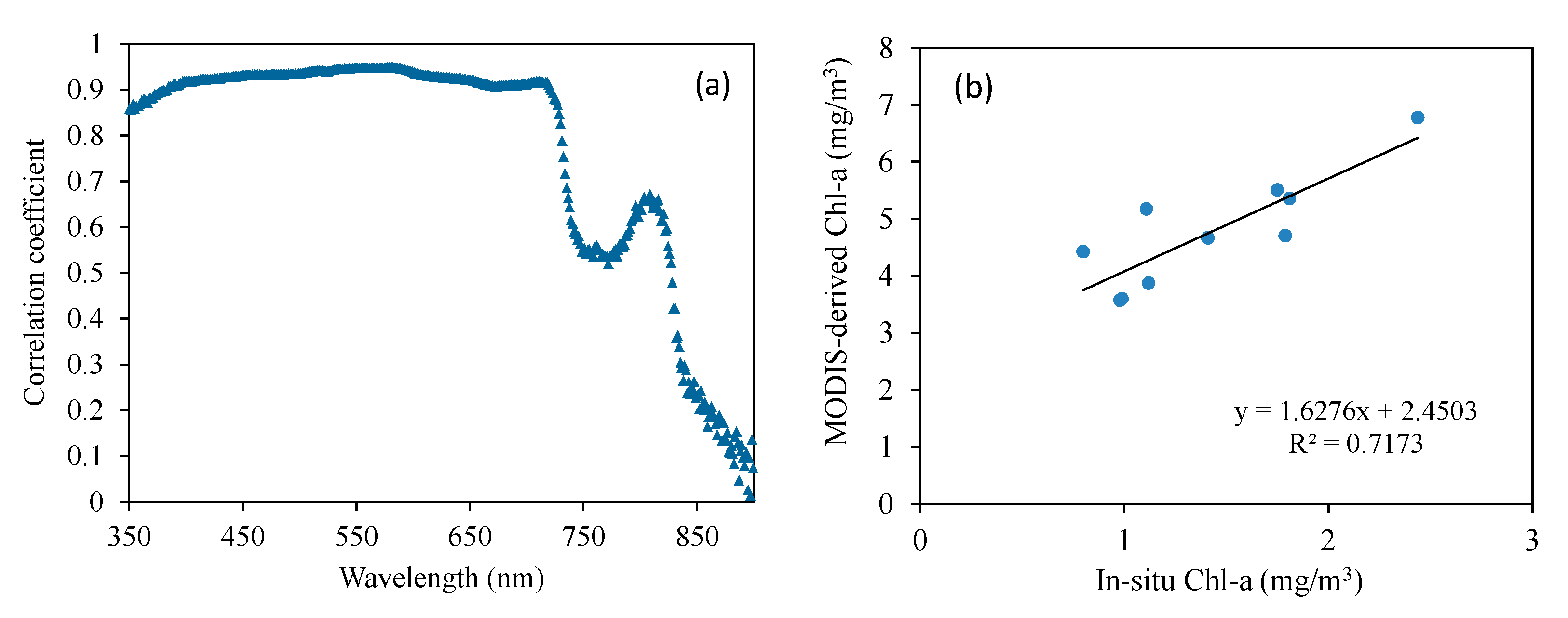
A particle size analysis of the suspended sediment samples was conducted using a Cilas 940L laser particle size meter (0.38–2000 μm) produced by Cilas, France. The particle size parameters were calculated using the moment method [23] to provide the average particle size, median particle size, sorting, skewness, and kurtosis. The sediment types were named based on Shepard (1954) [64].
The analysis and identification of detrital and clay minerals of suspended particulate matter was completed between December 2006 and April 2007 at the Marine Geological Testing Center of the Ministry of Land and Resources. The light and heavy minerals of the samples were identified using a binocular stereoscope, polarizing microscope, and by microanalysis [65]. A total of 300–500 particles were recorded using the strip number particle method, and the particle contents of the light and heavy minerals were calculated. The clay minerals were tested using a D/Max-rA X-ray diffractometer (Rigaku, Tokyo, Japan), details of the samples processes methodology can be found in Hu et al. (2018) [66]. After testing, the scanning images obtained were analyzed and compared with the relevant data to identify the clay mineral family to which the materials belonged. The Toussaint and Boniforti (2001) [67] method was used to assign the peak areas of the three characteristic diffraction peaks to four minerals: smectite, illite, chlorite, and kaolinite [68]. These data were used to calculate a semi-quantitative estimate of the clay mineral content [69].

2.6. MODIS Images

To compare the measured nearshore chlorophyll concentration with the estimated chlorophyll concentration by satellite, the MODIS image on 13 August 2011 in Heini Bay, China were selected and compared with the field measured chlorophyll concentration on 8 August 2011. The backscattering coefficients calculated from MODIS satellite data collected on 21 November 2004 and 2 May 2006 in Heini Bay, China were used for comparison with the results of Mie scattering calculations. The MODIS images on 4 August 2011, 17 August 2011, 23 August 2011, 26 August 2011, and 21 November 2011 in Heini Bay, China is used to retrieve particle size parameters of suspended particles and to monitor the influence range of typhoon.

3. Results

3.1. Parameter Determination

The chlorophyll concentration measured before the passage of typhoon Muifa on 8 August 2011, revealed the chlorophyll concentration measured in situ has a good correlation with the measured remote sensing reflectivity at 350–720 nm (Figure 2a). However, the comparison with MODIS inversion results on 13 August 2011 shows that MODIS overestimated the chlorophyll concentration value, which may be caused by the asynchronization of measurement and image time (Figure 2b). Therefore, the chlorophyll concentration data in this study were mainly obtained by using the inversion model constructed by measured data.
The Calis 940 L laser particle size analyzer sorts particles into 101 size ranges that are logarithmically distributed across a continuous size spectrum 0.38–2000 μm. Sixty-three of these particle size intervals were set to less than 100 μm. In this study, the particle size range was 0.5 to 95 μm. The final input required for the Mie scattering calculation of mineral particles was the particle size distribution and complex refractive index. The suspended particle sizes in this study area ranged from 0.5 to 71 μm, with significant peaks at 30 μm. The particle size distribution was dominated by single peaks, with a few secondary peaks. The concentration of suspended particulate matter ranged from 8.36 to 71.56 mg L−1, with an average of 23.16 mg L−1. Among the mineral particles present in this area, 96% were light minerals and 4% were heavy minerals. The light minerals were mainly feldspar (56%), quartz (28%), mica (0.58%), and carbonate (mainly calcite, 15%). Some stations contained trace amounts of chlorite and weathered mica. The heavy mineral components contributed 0–4% of the samples and were mainly common hornblende (39%), biotite (26%), green curtain (24%), and partial chlorite (11%) [70]. Based on Kerr (1977) [49], the real part of each mineral refractive index was calculated to be 1.144. Typical values vary between 1.03 and a theoretical upper limit of 1.158 for organic particles [71,72], depending on hydration, and between 1.07 and 1.22 for various minerals [28].

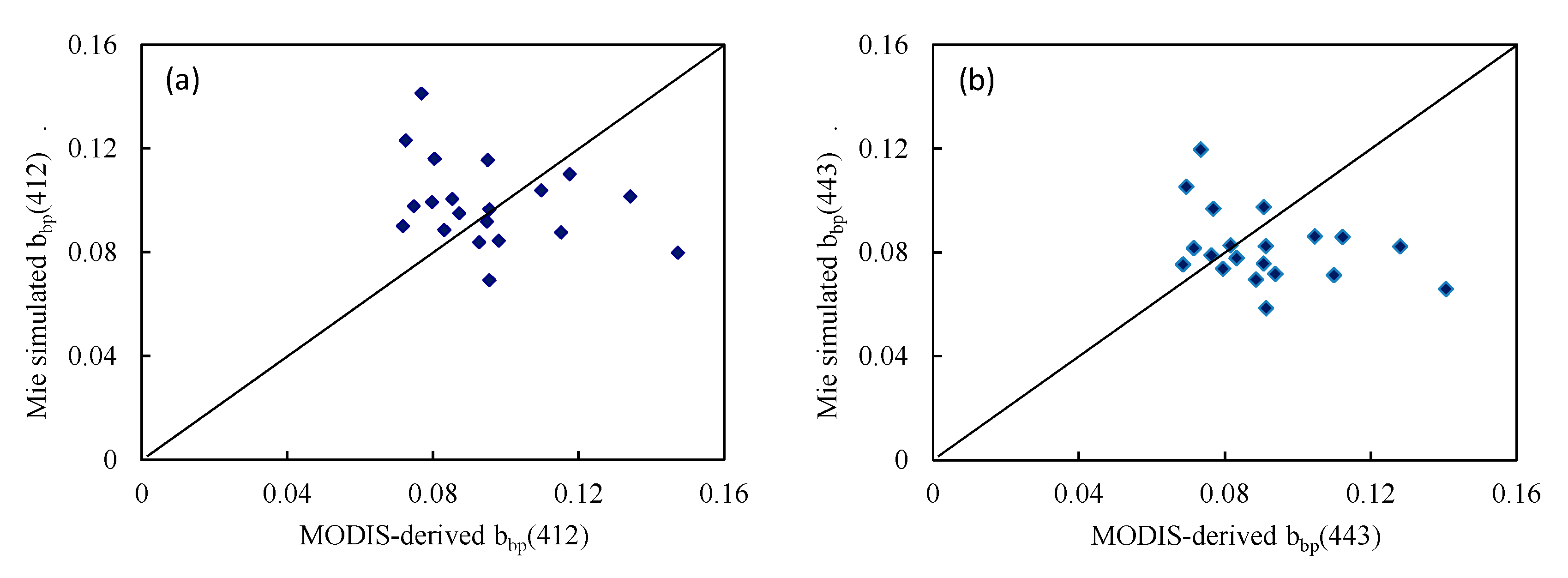
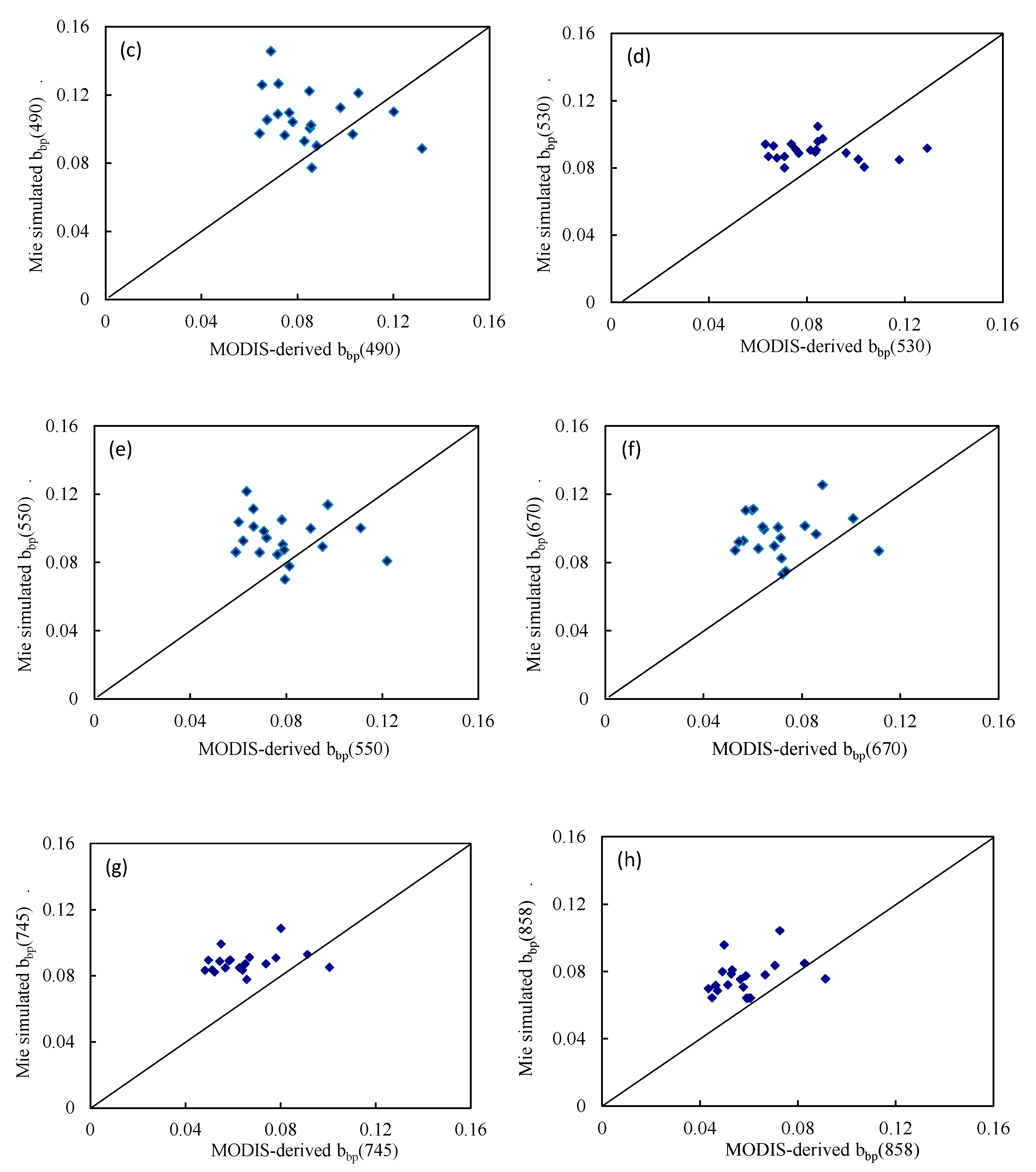
3.2. Calculation of the Backscattering Coefficient

The distribution function describing the volume percentages of suspended particulate matter obtained from on-site sampling and the backscattering efficiencies estimated by Mie scattering theory were used to estimate the backscattering coefficients of the suspended particulate matter using Equation (9). The input parameters provided in QAA V5 and Section 3.1 were used to estimate the backscattering coefficients of the suspended particulate matter over the wavelength range 412–865 nm in the MODIS satellite images. An example of a MODIS image taken on 21 November 2004 is presented herein. The estimation results, which did not consider absorption, indicated that the backscattering efficiency factor in this region oscillated with increasing particle diameter. For a fixed particle size, the backscattering efficiency factor decreased with increasing complex refractive index. Once the absorption was considered, however, the backscattering efficiency factor increased with the number of particles, and the particle diameters in this region were concentrated at about 30 µm.
A comparison of the backscattering coefficients estimated by Mie scattering theory and those retrieved by the MODIS images (Figure 3) revealed that the wavelengths 412, 443, 645, 745, and 858 nm were not sensitive to changes in the Mie scattering refractive index. By contrast, in several other sensitive bands, the range over which the backscattering coefficients estimated by Mie scattering varied was smaller than that estimated by the MODIS inversion. The values and ranges of the backscattering coefficients of the suspended particulate matter measured in this region [42] indicated that the estimated backscattering coefficients based on Mie scattering and the QAA algorithm were closer to the measured results. The two algorithms did deviate from the measured results; however, possibly due to atmospheric correction errors in the MODIS remote sensing reflectance product, the selection of empirical parameters in the QAA algorithm, and a lack of synchronization over the field-measured data.

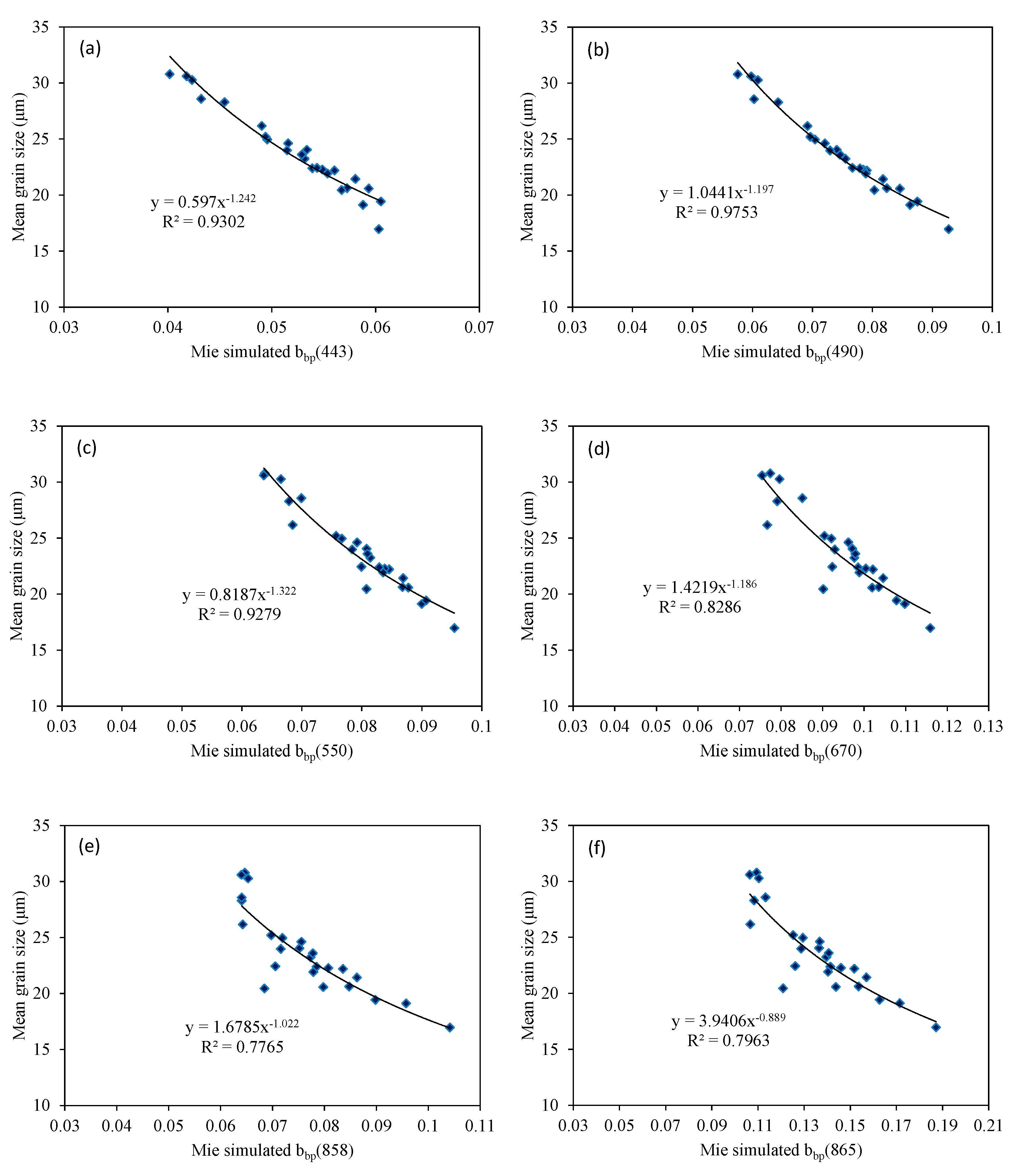
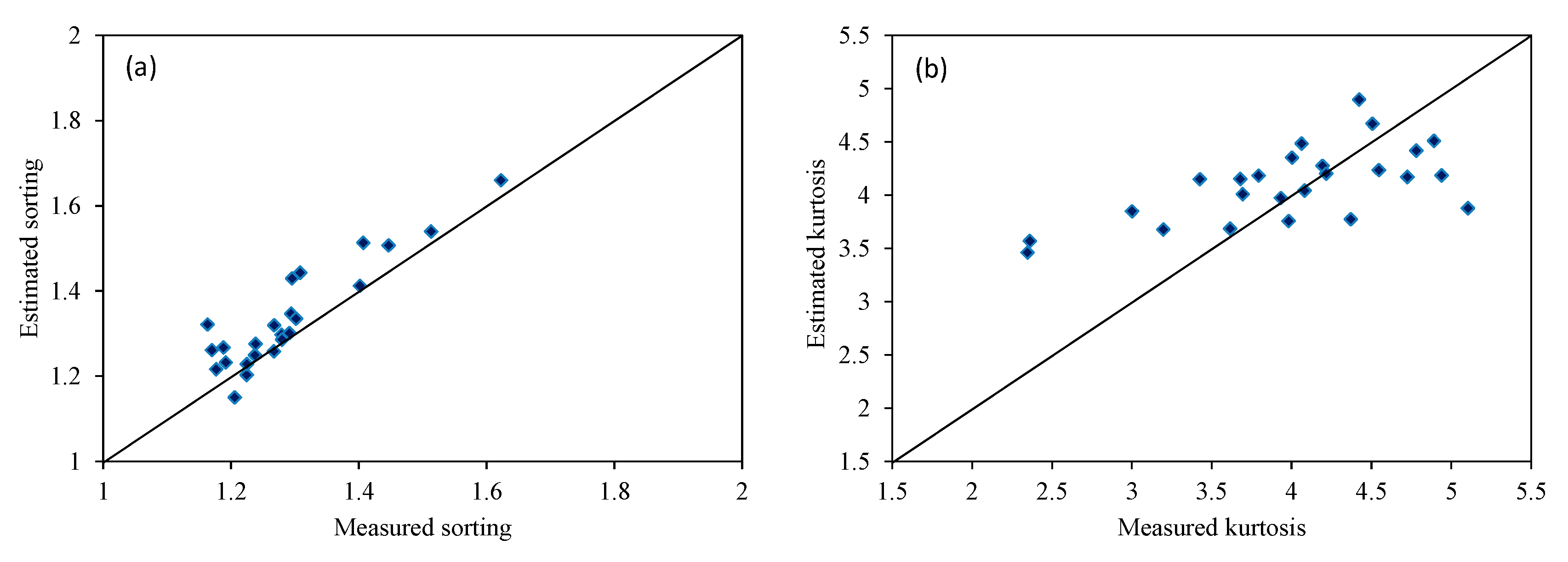
3.3. Calculation of the Suspended Particle Size Parameters

The backscattering efficiency and backscattering coefficient estimated by the Mie scattering and QAA algorithms in the previous section were next verified. The parameters describing the suspended particles, including the average particle size, sorting, skewness, and kurtosis, were calculated using the LSQR solution equation using the backscattering coefficient retrieval from the MODIS images and the backscattering efficiency factor estimated by Mie scattering. During the calculation process, the MODIS images were selected from 12 wavebands ranging from 412 nm to 868 nm, and the wavebands were selected mainly based on the light scattering characteristics of the visible and near-infrared wavebands in coastal waters in previous studies [28,73]. The results showed that the average particle size of suspended particles was correlated with the simulated backscattering coefficient (Figure 4). In this paper, the power exponential relationship between the average particle size and backscattering was assumed, and the dependence of backscattering on the wavelength was better in the visible light band than in the near-infrared band.
The sorting, skewness, and kurtosis of the suspended particles did not depend on the backscattering coefficient. Therefore, we used the LSQR solution to estimate the particle size parameters and compared the calculated results with the measured results. The estimated sorting and kurtosis results agreed well with the measured results. The estimated sorting results agreed most closely with the experimental results, whereas the estimated skewness results were larger than the experimental results, indicating that the coarse particle content was overestimated (Figure 5).

4. Discussion

4.1. Effects of the Mie Scattering input Parameters

During the seaweed farming season, the organic component of suspended particulate matter in this region can reach up to 20%, whereas during the non-farming season, it can be as low as 3.9% [56]. The results of previous laboratory experiments suggest that the scattering coefficient of suspended particles increases with increasing concentration, whereas the absorption decreases [74]. The range of refractive indices can be estimated in advance according to the scale and content of these suspended particles [75]. The mineral composition test results over this area revealed that the materials in this area mainly originated from the long-distance transport of materials from the Yellow River [58]. The suspended material composition in this area was similar to that in the South Yellow Sea, as indicated by the inorganic particulate matter absorption coefficient measured from the South Yellow Sea, which, in 2004, was less than 0.4 m−1 [42,47]. The range of the imaginary part of the refractive index could be obtained by optimizing the absorption coefficient [76,77]. Finally, these parameters were used in the Mie scattering estimation model. The measured suspended particle size distribution function was then used to estimate the backscattering coefficients of the suspended particles, which were in good agreement with the results obtained from the MODIS image. The composition, content, and distribution of mineral particles were used to obtain the backscattering input parameters, which indicated interdependence between the near-shore mineral particles and the inherent optical characteristic parameters of the water body. The particle size parameters (average particle size, sorting, skewness, and kurtosis) were used to characterize the particle distribution characteristics, and their changes altered the optical properties of the water. These results established an estimation relationship.

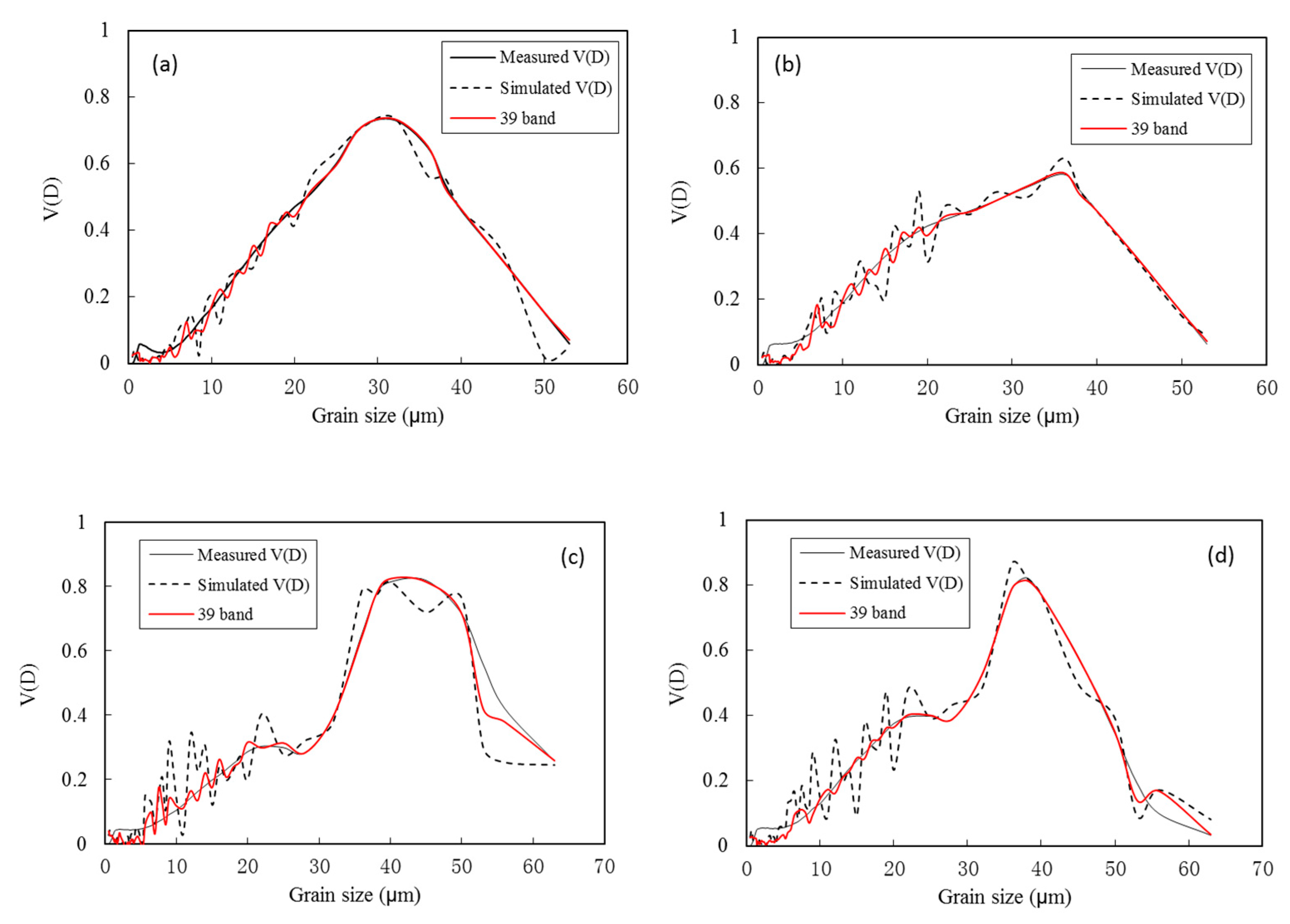
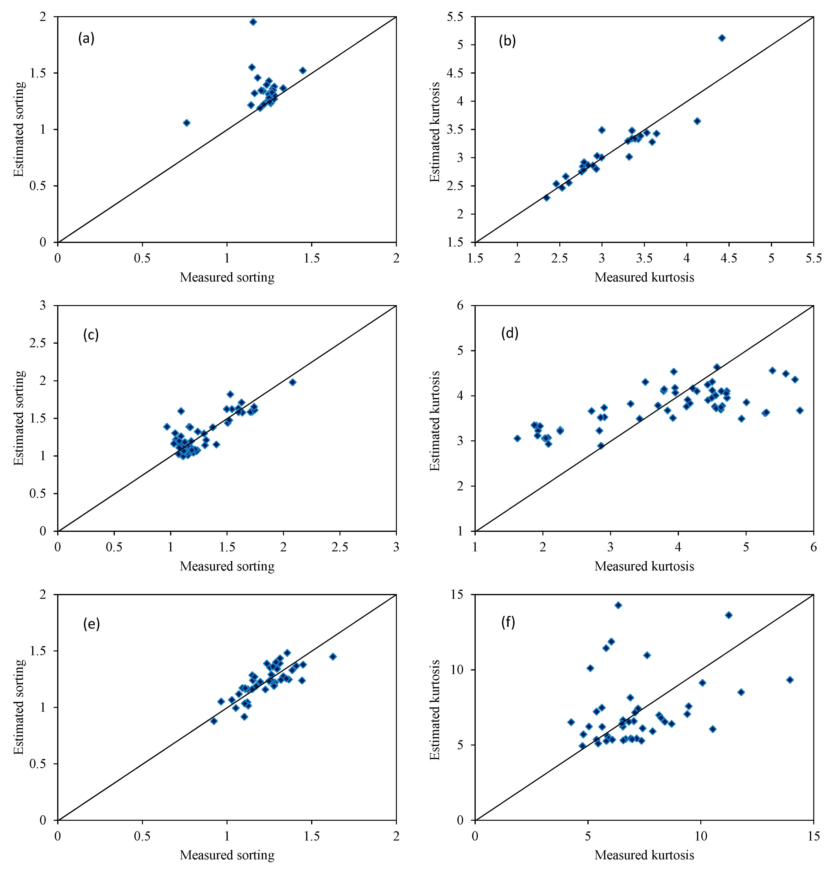
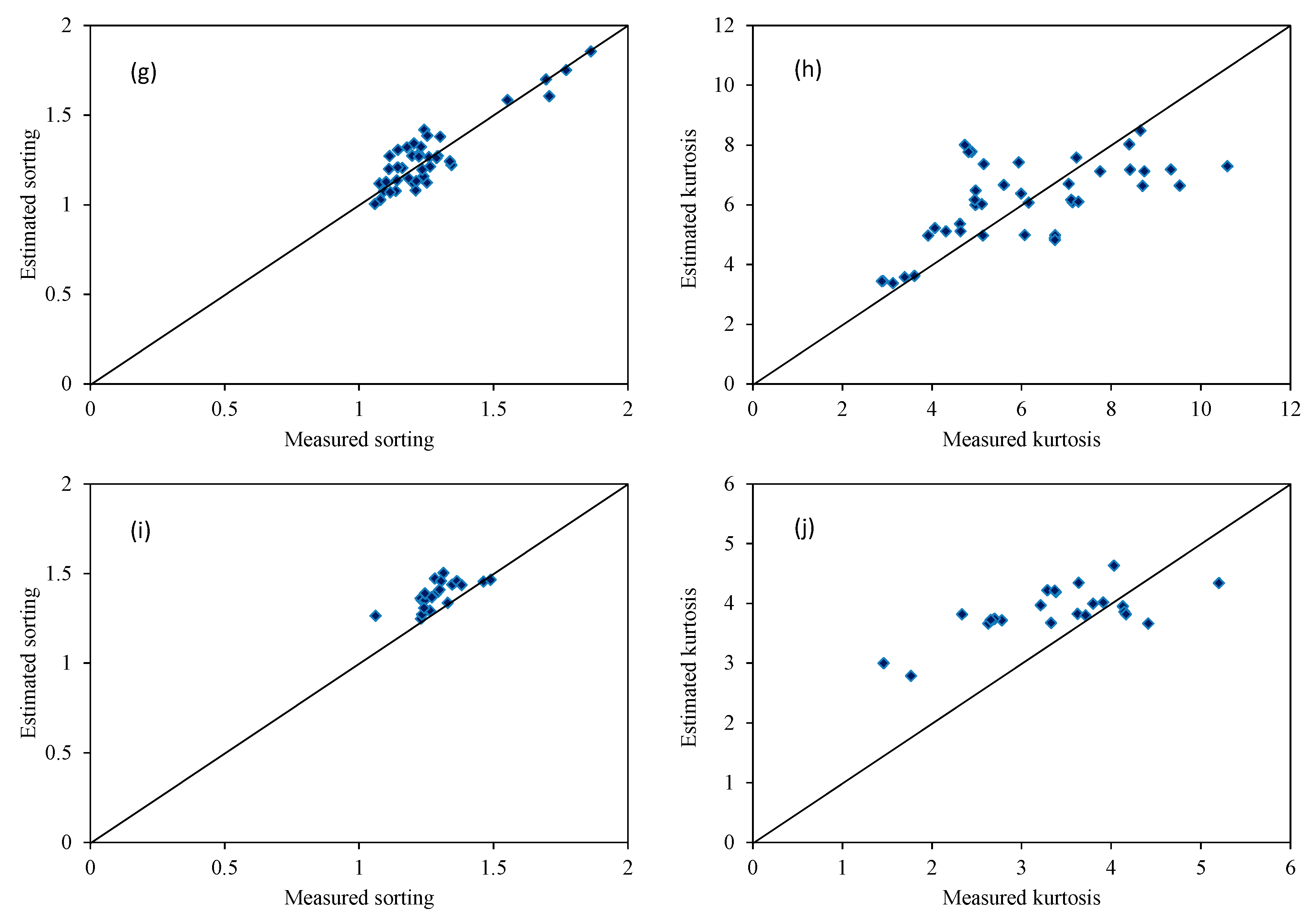
4.2. Estimation of the Particle Size Distribution

The relationship between the optical properties of water and the size distribution characteristics of the mineral particles was used to calculate the particle size distribution of particulate matter using the method of simulated estimation. An input wavelength range of 400 nm to 900 nm was used (the range used in previous studies [52], and 100 nm was set as the interval). The simulation results, however, were poor. This study further selected 19 bands between 400 nm and 2135 nm, corresponding to the MODIS band, as the input bands. The strong absorption effect of water on the MODIS data beyond 900 nm was considered by assuming that the reflectances of the 19 bands were non-zero. The measured particle volume percentage distribution was used as the input parameter, and the backscattering coefficient of the particles was calculated. The backscattering coefficient and the estimated backscattering efficiency factor were used to obtain the simulated particle volume percentage content using the LSQR solution equation. The results estimated using the measured PSD as input parameters differed from the measured results as a result of the number and spacing of the selected bands. We extended the simulation parameters to 412 nm and used 50 nm intervals to find better agreement between the 39-waveband simulation at 1830 nm and the measured results. An oscillation observed at < 20 µm did not disappear with the use of a greater number of bands. The > 53 µm estimation error was relatively large, possibly due to the selection of the Mie scattering input parameters (Figure 6).
The above experiments revealed that a relatively satisfactory model could be obtained using 39 bands separated by intervals of 50 nm. Certain assumptions in this simulation were not valid in the actual spectral measurements; therefore, we concluded that the band input limitations prevented direct calculation of the distribution curve of particles using the method of least squares.
Under many conditions, the PSD and its variations may be sufficiently quantified by focusing on such parameters as the median particle size of the PSD or other non-parametric descriptors, rather than by pursuing an accurate description of the PSD. This approach has been shown to provide sufficient information [5]. Therefore, the main purpose of this study was to obtain parameters that characterized the particle size distribution curve trends. Field measurements of the spectral data and MODIS images of the band set, with a total of 12 bands (412, 443, 469, 490, 530, 550, 645, 667, 680, 748, 858, 868 nm) were selected as input bands to estimate the particle size parameters. We estimated the particle size parameters of suspended particulate matter in the study area on 21 November 2004 (Figure 4) and found a strong correlation between the average particle size and the backscattering coefficient, which could be estimated without the least squares method. The sorting and kurtosis estimates were better, whereas the skewness estimates were worse. The estimated results were verified by selecting the reflectivity and particle size data measured on site over the periods 19–27 June 2004 and September 2012 in the Yellow River estuary, 12–23 June 2018, and 15 October through 12 November 2018 in the Bohai Sea, and 2–27 September 2003 in the Yellow Sea (Figure 7). The mineral composition and particle absorption coefficient in the Yellow River estuary and the Bohai Sea reported by Luo (2018) [78] were used in this work.
The validated calculated sorting and kurtosis particle size parameters agreed well with the measured results (Figure 7). The MODIS band settings, therefore, can be used as input parameters to estimate the sorting and kurtosis particle size parameters.

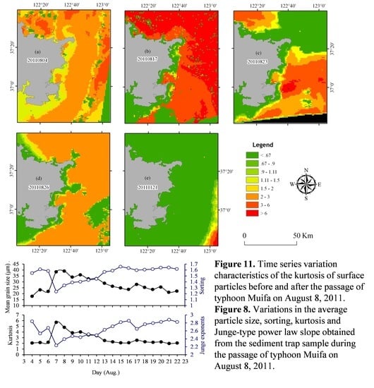
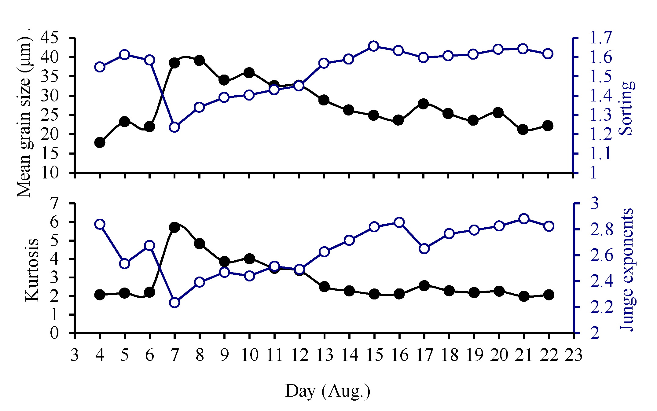
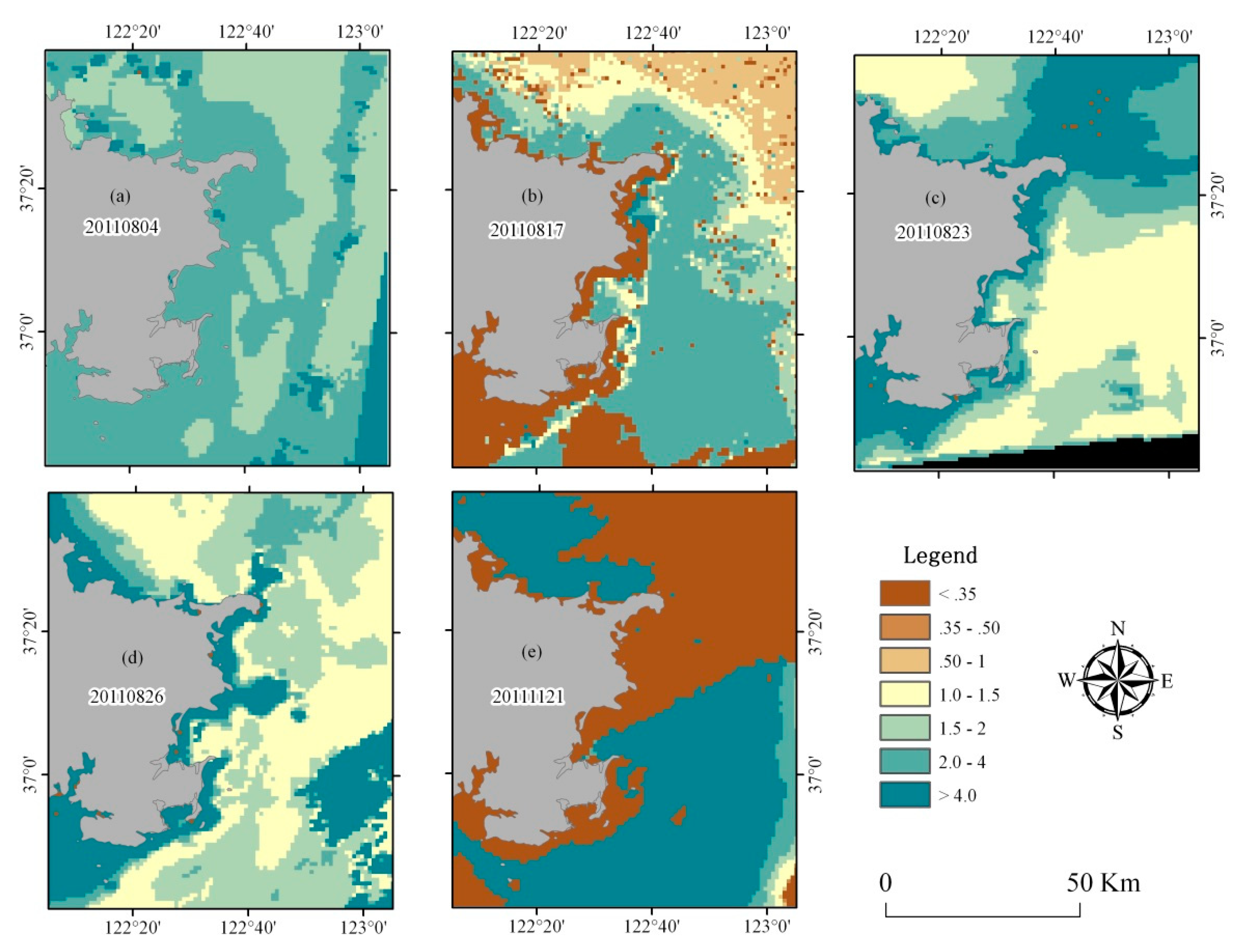
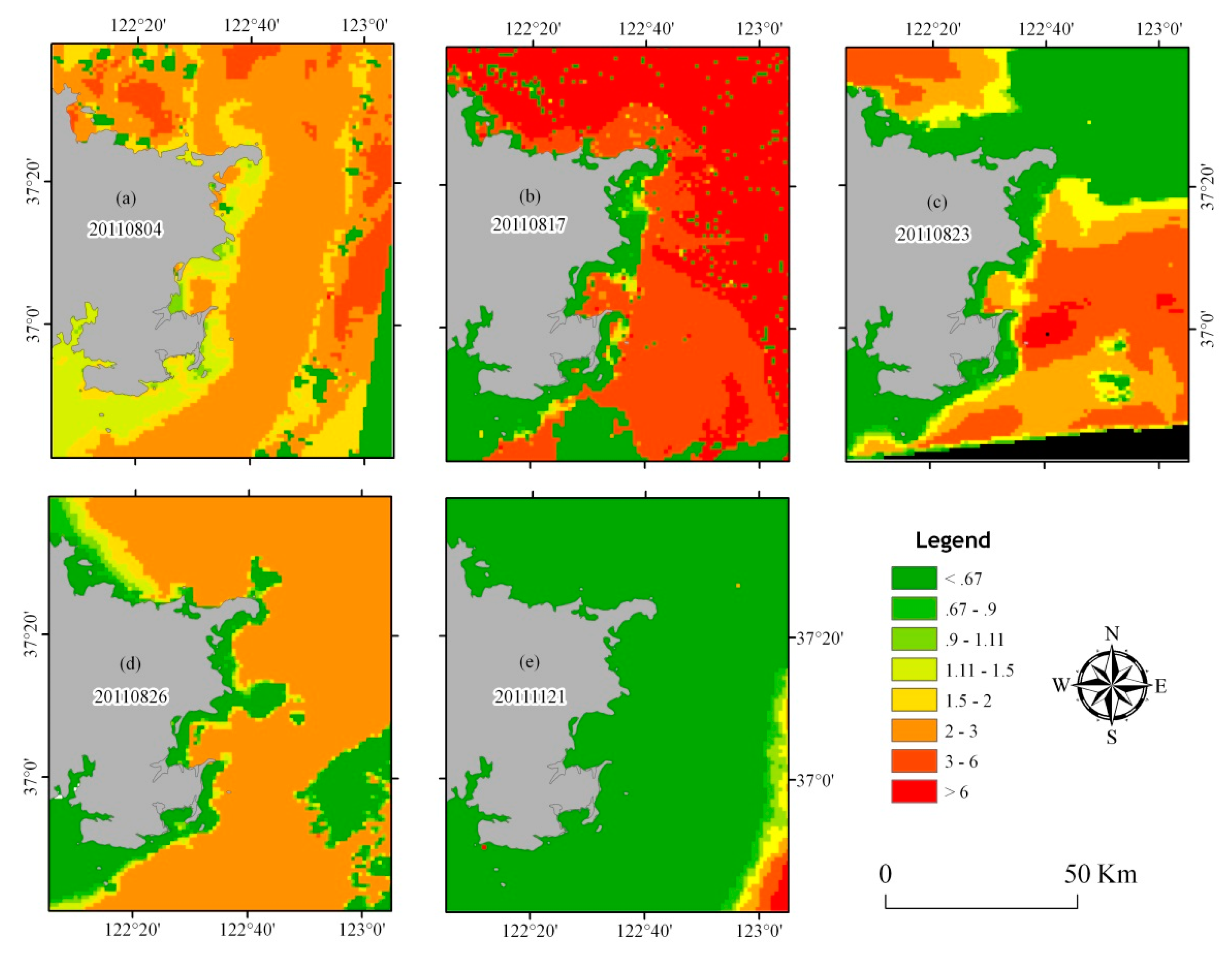
4.3. Estimated Particle Size Parameters around the Typhoon Impact

The distribution of sediment grain size, a basic physical property, varies with the hydrodynamic characteristics of sediment transport and deposition [21]. The sorting, skewness, and kurtosis of the particle size parameters are good indicators of the particulate matter changes after an environmental event. For example, during the passage of the typhoon Muifa in this study area on 8 August 2011, the suspended particle sizes monitored by the near-shore sediment trap revealed delayed coarsening, better sorting, more positive skewness, and more leptokurtic kurtosis. These characteristics suggested that the passage of the typhoon prolonged the in situ particle suspension time or moved the particles to the surrounding sea, resulting in a relative increase in the coarse particle composition of the local suspended particles. Power-law PSD slope is also used to characterize the changes of suspended particles before and after the passage of typhoon Muifa, indicating that the PSD slope of suspended particles decreases during typhoon transit, which means the content of coarse particles increases. The significance of this feature is the same as that of the skewness indicator (Figure 8 and Figure 3 in Liu et al. 2019 [63]). However, only the PSD slope parameter, as an indicator, is limited in identifying the environmental dynamic conditions that affect particle changes. We fully explained the environmental dynamic conditions of the particulate matter using the three indices of the average particle size, sorting, and kurtosis. These three parameters could also be obtained from a sediment core sample [56,63], which can provide a link between the distribution characteristics of the modern sediments monitored by remote sensing and the historical sedimentary record.

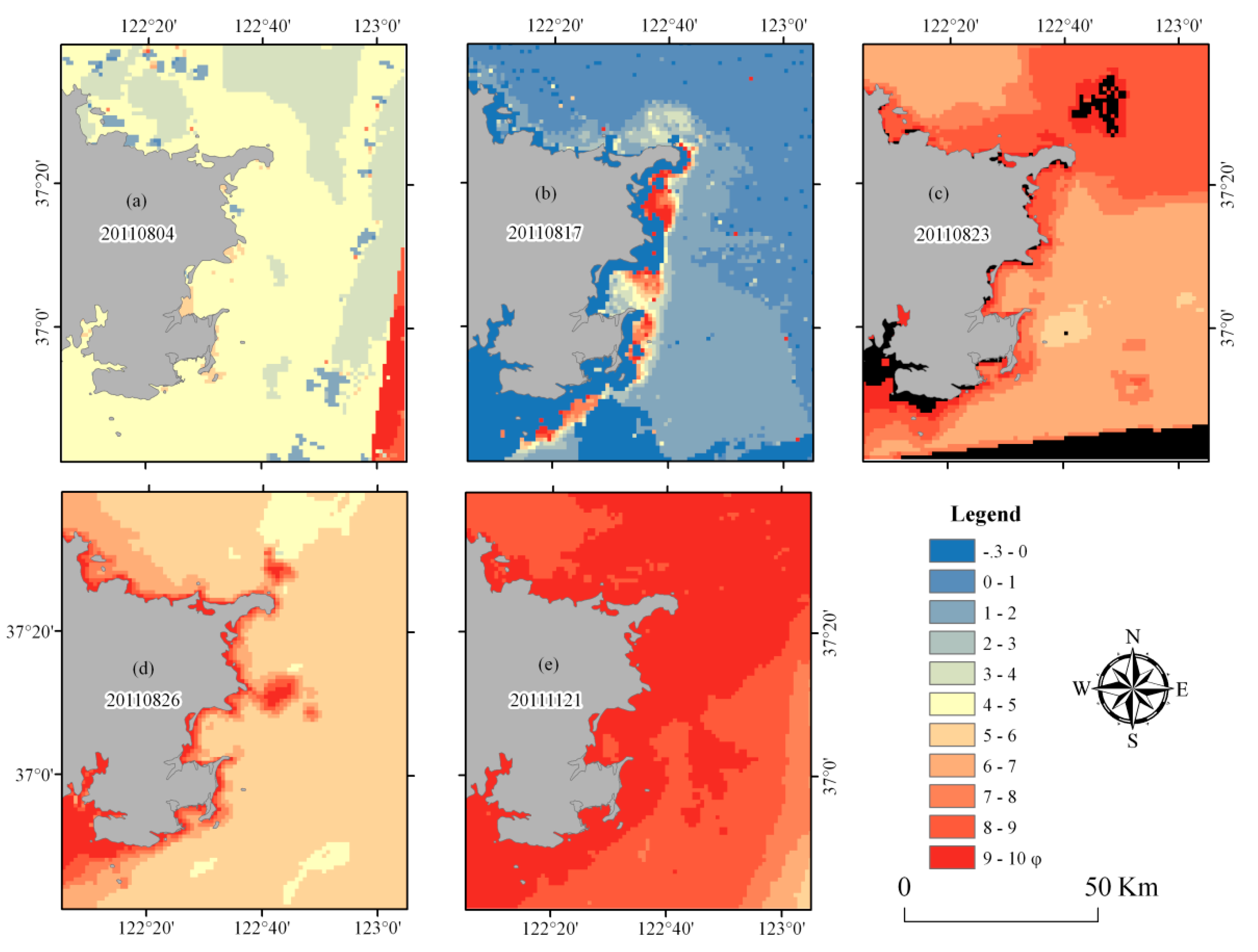
4.4. Monitoring the Typhoon Impact Range

The analysis results discussed above were used to invert and estimate the average particle size (ø), sorting, and kurtosis of the suspended sediment in the waters around Heini bay before and after the passage of typhoon Muifa on 8 August 2011. The average particle size inversion revealed that the average particle size over the entire studied area was 4–5 ø on 4 August 2011 before the arrival of the typhoon (Figure 9), slightly coarser than the average particle size of 5–6 ø obtained during the winter survey in 2004. The results estimated from the 17 August 2011 imaging data indicated that the suspended particulate matter over a large area of the sea was coarsened to 3–4 ø, and by 23 and 26 August 2011, the particle sediment has been re-refined to 5–6 ø (Figure 9). Please note that the image collected closest to the typhoon passage and unobstructed by clouds was collected on 17 August 2011. The typhoon transit also changed the characteristics of the suspended particulate distribution curve from 10 to 18 August 2011 in that the grain size distribution curve over this area displayed a leptokurtic peak from strong to weak (see Figure 4 in Liu et al., 2019 [63] for details). The results were verified by comparing MODIS data with good image quality, collected on 21 November 2011, and the sampling data collected on 28 November 2011 (see Figure 5 in Liu et al., 2019 [63] for details). It was found that three months after the passage of the typhoon, the surface suspended sediment comprised mainly fine particles. (Please note that the northeastern part of the image was affected by clouds, so the estimation accuracy was slightly reduced). This distribution was consistent with the coarsening of suspended sediment particles during extreme weather events.
Similarly, the sorting retrieval results of suspended particulate matter revealed that on 4 August 2011, before the passage of the typhoon, the sorting of suspended sediment was 1.5–4 (Figure 10), which was poor to very poor (Table 1). These results resembled the field survey results (Figure 8). On 17 August 2011, after the passage of typhoon, the sorting of suspended sediment improved significantly, and the sorting across most areas in the coastal sea and the outer sea was moderate to good (Table 1). On 23 and 26 August 2011, the sorting gradually worsened. On 21 November 2011, three months after the typhoon passage, the sorting of suspended sediment returned to the poor state under normal weather conditions. The characteristics of this time series are consistent with prior observations that a typhoon will improve the sorting of suspended sediment.
The kurtosis of the suspended particulate matter on 4 August before the passage of the typhoon was 1.5–3 (Figure 11), indicating a very leptokurtic type (Table 1). The average value was similar to the measured results (Figure 8). On 17 August 2011, after the typhoon passage, kurtosis in this area was 3–6 or greater than 6, except over a large area in the coastal sea, which belonged to the extremely leptokurtic type (Table 1). These results were in agreement with the characteristics of extreme coarsening among suspended matter caused by the passage of a typhoon. The sediments in the headland of bedrock were mostly coarse particles, and the influence of the typhoon on the suspended sediment was not significant. This observation was consistent with the non-significant changes observed in the near-shore particulate matter, as demonstrated in Figure 5 of Liu et al. (2019) [63]. With the gradual weakening of the typhoon’s influence, the leptokurtic characteristics of the suspended grain size distribution curve gradually weakened on 23 and 26 August 2011. Similarly, the changes along the coastal waters remained insignificant. On 21 November 2011, three months after the typhoon passage, the kurtosis of the suspended particles was characterized by a platykurtic type of less than 0.9 (Table 1). These change characteristics also indicated that in the absence of a strong dynamic influence in the area, the suspended particle size distribution curve, which was platykurtic type (Table 1), was consistent with the particle size characteristics under normal weather conditions (see Figure 4 and Figure 10 in Liu, et al., 2019 [63] for details).
In summary, the MODIS estimates of the average particle size (ø), sorting, and kurtosis in the surface suspended sediment in the area near Heini Bay before and after the passage of typhoon Muifa in August 2011 indicate that the influence of the typhoon increased the average particle size, reduced the sorting coefficient, and shifted the distribution curve of particulate matter toward the leptokurtic type. The strong dynamic effect of the typhoon did not significantly affect the coarse sediment near the shore, although the typhoon significantly affected a large area in its pathway. The estimation results indicated that the typhoon created a strong ocean power that resuspend the coarse sediment of the seabed, thereby improving the sorting of suspended sediment. The estimated particle size parameter characteristics were comparable to the experimental sediment characteristics measured from the sediment trap sample (as described in Figure 3 and Figure 4 in Liu et al., 2019 [63]). The estimated characteristics of the sediment particle size parameters also agreed with the experimental seabed historical sediment records (see Figure 10 in Liu et al., 2019 [63] for details). Because the field-measured data used in this study only covered the coastal waters of Heini Bay, the image-based estimates of the typhoon transit only encompassed the waters around Heini Bay. The image quality and other factors could be improved in future studies to survey the full typhoon impact area. To improve the inversion of the water-bearing components in other environments, including coastal and estuarine systems, the algorithms should be optimized using in situ regional measurements of optical and biogeochemical water characteristics. Nevertheless, for the purposes of monitoring in this study, the sediment particle size parameters estimated from remote sensing images do indeed reflect the environmental impact of strong marine dynamic events over a specific region.

5. Conclusions

In this study, we calculated the particle size parameters often used in sedimentary geology based on the suspended particle optical properties and Junge power law distribution relationship. We found that the average suspended particulate matter grain size (ø value), sorting, and kurtosis values obtained from MODIS remote sensing image estimation methods agreed well with the experimental values. During the estimation process, the mineral composition of the suspended particulate matter in the region should be obtained first to determine the real part of the complex refractive index used in the Mie scattering model. The absorption and scattering coefficients of the water components may be estimated using the QAA analysis algorithm. Therefore, the model is universal in its applicability. The results were verified in several coastal areas of China and were found to be satisfactory. On the other hand, the LSQR method used in the model may simulate a better particle distribution curve in the short-wave infrared band with 39 bands of visible light up to 1830 nm (50 nm intervals). Given experimental limitations, however, the water color in the MODIS data may be used together with the terrestrial application band to improve the results. Therefore, the estimation accuracy is greatly affected by the number of wavebands included.
We selected images before and after the passage of a typhoon to estimate changes in the particle size parameters describing surface suspended sediment in a coastal area under the influence of strong ocean dynamics. Field measurements revealed that these three parameters accurately represented changes in the suspended particulate matter in coastal waters. The study also found that the power law PSD slope could be interpreted as an indicator of the skewness. These parameters, therefore, could be used together to characterize suspended particulate matter variations in coastal areas, compensating for the uncertainty of a single indicator of the PSD slope. The quality of images collected during the passage of a typhoon will be limited by the presence of typhoon weather clouds and other factors. This method, therefore, requires further verification with consideration for human activities and other variable environmental effects. Nevertheless, the method of estimating the particle size parameters in sedimentary geology using remote sensing proposed in this paper is of practical value for establishing the relationship between parameters in remote sensing monitoring and in the sedimentary records. This method also provides a new application of the power law model in the near-shore environment.

Author Contributions

Conceptualization, Y.L. and H.H.; methodology, Y.L.; software, Y.L. and H.B.; validation, X.Y., L.Y. and Z.Z.; formal analysis, Y.L.; investigation, L.Y.; resources, Y.L.; data curation, Y.L.; writing—original draft preparation, Y.L.; writing—review and editing, Y.L.; visualization, X.Y.; supervision, H.H.; project administration, H.H.; funding acquisition, H.H. All authors have read and agreed to the published version of the manuscript.

Funding

This research was funded by the National Natural Science Foundation of China (NSFC), grant number 41976166 and the NSFC–Shandong Joint Fund for Marine Science Research Centers, grant number U1606401.

Acknowledgments

The authors would like to thank NASA Ocean colors for providing MODIS data.

Conflicts of Interest

The authors declare no conflict of interest.

References

  1. Boss, E.; Pegau, W.S.; Gardner, W.D.; Zaneveld, J.R.V.; Barnard, A.H.; Twardowski, M.S.; Chang, G.; Dickey, T. Spectral particulate attenuation and particle size distribution in the bottom boundary layer of a continental shelf. J. Geophys. Res. Ocean. 2001, 106, 9509–9516. [Google Scholar] [CrossRef] [Green Version]
  2. Loisel, H.; Nicolas, J.M.; Sciandra, A.; Stramski, D.; Poteau, A. Spectral dependency of optical backscattering by marine particles from satellite remote sensing of the global ocean. J. Geophys. Res. Ocean. 2006, 111, 1–14. [Google Scholar] [CrossRef]
  3. Kostadinov, T.; Siegel, D.; Maritorena, S. Retrieval of the particle size distribution from satellite ocean color observations. J. Geophys. Res. Ocean. 2009, 114, 1–22. [Google Scholar] [CrossRef]
  4. Aurin, D.A.; Dierssen, H.M. Advantages and limitations of ocean color remote sensing in CDOM-dominated, mineral-rich coastal and estuarine waters. Remote Sens. Environ. 2012, 125, 181–197. [Google Scholar] [CrossRef]
  5. Slade, W.H.; Boss, E. Spectral attenuation and backscattering as indicators of average particle size. Appl. Opt. 2015, 54, 7264–7277. [Google Scholar] [CrossRef]
  6. International Ocean-Colour Coordinating Group. Remote Sensing of Ocean Colour in Coastal, and other optically complex, waters. In Reports of the International Ocean-Colour Coordinating Group Nr 3 IOCCG; IOCCG: Dartmouth, NS, Canada, 2000. [Google Scholar]
  7. Soja-Wozniak, M.; Baird, M.; Schroeder, T.; Qin, Y.; Clementson, L.; Baker, B.; Boadle, D.; Brando, V.; Steven, A.D.L. Particulate Backscattering Ratio as an Indicator of Changing Particle Composition in Coastal Waters: Observations From Great Barrier Reef Waters. J. Geophys. Res. Ocean. 2019, 124, 5485–5502. [Google Scholar] [CrossRef]
  8. Stramski, D.; Woźniak, S.B.; Flatau, P.J. Optical properties of Asian mineral dust suspended in seawater. Limnol. Oceanogr. 2004, 49, 749–755. [Google Scholar] [CrossRef]
  9. Stramski, D.; Kiefer, D.A. Light scattering by microorganisms in the open ocean. Prog. Oceanogr. 1991, 28, 343–383. [Google Scholar] [CrossRef]
  10. Morel, A.; Prieur, L. Analysis of Variation in Ocean Color. Limnol. Oceanogr. 1977, 22, 709–722. [Google Scholar] [CrossRef]
  11. Stavn, R.H.; Keen, T.R. Suspended minerogenic particle distributions in high-energy coastal environments: Optical implications. J. Geophys. Res. Ocean. 2004, 109, 1–14. [Google Scholar] [CrossRef] [Green Version]
  12. Buonassissi, C.; Dierssen, H. A regional comparison of particle size distributions and the power law approximation in oceanic and estuarine surface waters. J. Geophys. Res. Ocean. 2010, 115, 1–12. [Google Scholar] [CrossRef]
  13. Medina, R.; Losada, M.A.; Losada, I.J.; Vidal, C. Temporal and spatial relationship between sediment grain size and beach profile. Mar. Geol. 1994, 118, 195–206. [Google Scholar] [CrossRef]
  14. Stauble, D.K.; Cialone, M.A. Sediment dynamics and profile interactions: Duck94. Coast. Eng. 1996, 4, 3921–3934. [Google Scholar]
  15. Zhao, Y.; Zou, X.; Gao, J.; Wang, C. Recent sedimentary record of storms and floods within the estuarine-inner shelf region of the East China Sea. Holocene 2017, 27, 439–449. [Google Scholar] [CrossRef]
  16. Swindles, G.T.; Galloway, J.M.; Macumber, A.L.; Croudace, I.W.; Emery, A.R.; Woulds, C.; Bateman, M.D.; Parry, L.; Jones, J.M.; Selby, K.; et al. Sedimentary records of coastal storm surges: Evidence of the 1953 North Sea event. Mar. Geol. 2018, 403, 262–270. [Google Scholar] [CrossRef]
  17. Sahu, B.K. Depositional mechanisms from the size analysis of clastic sediments. J. Sediment. Res. 1964, 34, 73–83. [Google Scholar]
  18. Xiang, R.; Yang, Z.; Saito, Y.; Guo, Z.; Fan, D.; Li, Y.; Xiao, S.; Shi, X.; Chen, M. East Asia Winter Monsoon changes inferred from environmentally sensitive grain-size component records during the last 2300 years in mud area southwest off Cheju Island, ECS. Sci. China Ser. D 2006, 49, 604–614. [Google Scholar] [CrossRef]
  19. Judd, K.; Chagué-Goff, C.; Goff, J.; Gadd, P.; Zawadzki, A.; Fierro, D. Multi-proxy evidence for small historical tsunamis leaving little or no sedimentary record. Mar. Geol. 2017, 385, 204–215. [Google Scholar] [CrossRef]
  20. Puerres, L.Y.; Bernal, G.; Brenner, M.; Restrepo-Moreno, S.A.; Kenney, W.F. Sedimentary records of extreme wave events in the southwestern Caribbean. Geomorphology 2018, 319, 103–116. [Google Scholar] [CrossRef]
  21. Watson, E.B.; Pasternack, G.B.; Gray, A.B.; Goñi, M.; Woolfolk, A.M. Particle size characterization of historic sediment deposition from a closed estuarine lagoon, Central California. Estuar. Coast. Shelf Sci. 2013, 126, 23–33. [Google Scholar] [CrossRef]
  22. Folk, R.L.; Ward, W.C. Brazos River bar: A study in the significance of grain size parameters. J. Sediment. Petrol. 1957, 27, 3–26. [Google Scholar] [CrossRef]
  23. McManus, J. Grain Size Determination and Interpretation. In Techniques in Sedimentology; Tucker, M., Ed.; Blackwell: Oxford, UK, 1988; pp. 63–85. [Google Scholar]
  24. Huisman, B.J.A.; de Schipper, M.A.; Ruessink, B.G. Sediment sorting at the Sand Motor at storm and annual time scales. Mar. Geol. 2016, 381, 209–226. [Google Scholar] [CrossRef]
  25. Sun, X.; Luo, Y.; Huang, F.; Tian, J.; Wang, P. Deep-sea pollen from the South China Sea: Pleistocene indicators of East Asian monsoon. Mar. Geol. 2003, 201, 97–118. [Google Scholar] [CrossRef]
  26. Huang, J.; Li, A.; Wan, S. Sensitive grain-size records of Holocene East Asian summer monsoon in sediments of northern South China Sea slope. Quat. Res. 2011, 75, 734–744. [Google Scholar] [CrossRef]
  27. Stramski, D.; Babin, M.; Woźniak, S.B. Variations in the optical properties of terrigenous mineral-rich particulate matter suspended in seawater. Limnol. Oceanogr. 2007, 52, 2418–2433. [Google Scholar] [CrossRef] [Green Version]
  28. Doxaran, D.; Ruddick, K.; McKee, D.; Gentili, B.; Tailliez, D.; Chami, M.; Babin, M. Spectral variations of light scattering by marine particles in coastal waters, from the visible to the near infrared. Limnol. Oceanogr. 2009, 54, 1257–1271. [Google Scholar] [CrossRef] [Green Version]
  29. Zhang, X.; Gray, D.J. Backscattering by very small particles in coastal waters. J. Geophys. Res. Ocean. 2015, 120, 6914–6926. [Google Scholar] [CrossRef] [Green Version]
  30. Pinet, S.; Martinez, J.-M.; Ouillon, S.; Lartiges, B.; Villar, R.E. Variability of apparent and inherent optical properties of sediment-laden waters in large river basins–lessons from in situ measurements and bio-optical modeling. Opt. Express 2017, 25, A283–A310. [Google Scholar] [CrossRef]
  31. Tao, J.; Hill, P.S.; Boss, E.S.; Milligan, T.G. Variability of Suspended Particle Properties Using Optical Measurements within the Columbia River Estuary. J. Geophys. Res. Ocean. 2018, 123, 6296–6311. [Google Scholar] [CrossRef]
  32. Zhang, Y.; Huang, Z.; Chen, C.; He, Y.; Jiang, T. Particle size distribution of river-suspended sediments determined by in situ measured remote-sensing reflectance. Appl. Opt. 2015, 54, 6367–6376. [Google Scholar] [CrossRef]
  33. Zhang, X.; Stavn, R.H.; Falster, A.U.; Gray, D.; Gould, R.W., Jr. New insight into particulate mineral and organic matter in coastal ocean waters through optical inversion. Estuar. Coast. Shelf Sci. 2014, 149, 1–12. [Google Scholar] [CrossRef] [Green Version]
  34. Bader, H. The hyperbolic distribution of particle sizes. J. Geophys. Res. 1970, 75, 2822–2830. [Google Scholar] [CrossRef]
  35. Hulst, H.C.V.D. Light Scattering By Small Particles. Phys. Today 1957, 10. [Google Scholar] [CrossRef]
  36. Bricaud, A.; Morel, A. Light attenuation and scattering by phytoplanktonic cells: A theoretical modeling. Appl. Opt. 1986, 25, 571–580. [Google Scholar] [CrossRef] [PubMed]
  37. Mobley, C.D. Light and Water: Radiative Transfer in Natural Waters; Academic: San Diego, CA, USA, 1994; p. 592. [Google Scholar]
  38. Reynolds, R.; Stramski, D.; Wright, V.; Woźniak, S. Measurements and characterization of particle size distributions in coastal waters. J. Geophys. Res. Ocean. 2010, 115. [Google Scholar] [CrossRef]
  39. Mohammadpour, G.; Gagné, J.-P.; Larouche, P.; Montes-Hugo, M.A. Optical properties of size fractions of suspended particulate matter in littoral waters of Québec. Biogeosciences 2017, 14, 5297–5312. [Google Scholar] [CrossRef] [Green Version]
  40. Stramski, D.; Bricaud, A.; Morel, A. Modeling the inherent optical properties of the ocean based on the detailed composition of the planktonic community. Appl. Opt. 2001, 40, 2929–2945. [Google Scholar] [CrossRef]
  41. Sathyendranath, S.; Prieur, L.; Morel, A. A 3-Component Model of Ocean Color and Its Application to Remote-Sensing of Phytoplankton Pigments in Coastal Waters. Int. J. Remote Sens. 1989, 10, 1373–1394. [Google Scholar] [CrossRef]
  42. Zhang, M.W.; Tang, J.W.; Dong, Q.; Song, Q.T.; Ding, J. Retrieval of total suspended matter concentration in the Yellow and East China Seas from MODIS imagery. Remote Sens. Environ. 2010, 114, 392–403. [Google Scholar] [CrossRef]
  43. Morel, A. Optical properties of pure seawater. In Optical Aspects of Oceanography; Jerlov, N.G., Steemann Nielson, E., Eds.; Academic Press: London, UK, 1974; pp. 1–24. [Google Scholar]
  44. Smith, R.C.; Baker, K.S. Optical properties of the clearest natural waters (200–800 nm). Appl. Opt. 1981, 20, 177–184. [Google Scholar] [CrossRef]
  45. Morel, A.; Gentili, B.; Claustre, H.; Babin, M.; Bricaud, A.; Ras, J.; Tièche, F. Optical Properties of the “Clearest” Natural Waters. Limnol. Oceanogr. 2007, 52, 217–229. [Google Scholar] [CrossRef]
  46. Lee, Z.P.; Carder, K.L.; Arnone, R.A. Deriving inherent optical properties from water color: A multiband quasi-analytical algorithm for optically deep waters. Appl. Opt. 2002, 41, 5755–5772. [Google Scholar] [CrossRef] [PubMed]
  47. Qing, S.; Tang, J.W.; Cui, T.W.; Zhang, J. Retrieval of inherent optical properties of the Yellow Sea and East China Sea using a quasi-analytical algorithm. Chin. J. Oceanol. Limnol. 2011, 29, 33–45. [Google Scholar] [CrossRef]
  48. Bohren, C.F.; Huffman, D.R.; Kam, Z. Book-Review—Absorption and Scattering of Light by Small Particles. Nature 1983, 306, 625. [Google Scholar]
  49. Kerr, P. Optical Mineralogy; McGraw Hill Book Company: New York, NY, USA, 1977; p. 492. [Google Scholar]
  50. Krumbein, W.C. Size Frequency Distributions of Sediments. J. Sediment. Res. 1934, 4, 65–77. [Google Scholar] [CrossRef]
  51. Yu, X.; Shi, Y.; Wang, T.; Sun, X. Dust-concentration measurement based on Mie scattering of a laser beam. PLoS ONE 2017, 12, e0181575. [Google Scholar] [CrossRef] [Green Version]
  52. He, Z.; Mao, J.; Han, X. Non-parametric estimation of particle size distribution from spectral extinction data with PCA approach. Powder Technol. 2018, 325, 510–518. [Google Scholar] [CrossRef]
  53. Paige, C.C.; Saunders, M.A. LSQR: An algorithm for sparse linear equations and sparse least squares. ACM Trans. Math. Softw. 1982, 8, 43–71. [Google Scholar] [CrossRef]
  54. Golub, G.; Kahan, W. Calculating the singular values and pseudo-inverse of a matrix. J. Soc. Ind. Appl. Math. Ser. B Numer. Anal. 1965, 2, 205–224. [Google Scholar] [CrossRef]
  55. Liu, J.; Saito, Y.; Kong, X.; Wang, H.; Zhao, L. Geochemical characteristics of sediment as indicators of post-glacial environmental changes off the Shandong Peninsula in the Yellow Sea. Cont. Shelf Res. 2009, 29, 846–855. [Google Scholar] [CrossRef]
  56. Liu, Y.; Huang, H.; Yan, L.; Liu, X.; Zhang, Z. Influence of suspended kelp culture on seabed sediment composition in Heini Bay, China. Estuar. Coast. Shelf Sci. 2016, 181, 39–50. [Google Scholar] [CrossRef]
  57. SPSTC (Shandong Province Science and Technology Committee). Collection of Research Reports on Coastal Zone and Tidal Flat Resources in Shandong Province; Chinese Science and Technology Press: Beijing, China, 1991. (In Chinese) [Google Scholar]
  58. Yan, L.W. Sedimentary Environment Evolution in Representative Kelp (Laminaria Japonica)-Cultured Region (Harny Bay); The Thesis of Doctor’ Degree of University of Chinese Academy of Sciences: Beijing, China, 2008; pp. 35–40, (In Chinese with English abstract). [Google Scholar]
  59. Hu, L.; Shi, X.; Guo, Z.; Wang, H.; Yang, Z. Sources, dispersal and preservation of sedimentary organic matter in the Yellow Sea: The importance of depositional hydrodynamic forcing. Mar. Geol. 2013, 335, 52–63. [Google Scholar] [CrossRef]
  60. Gao, X.M.; Jiang, J.; Ma, S.Q.; Xu, W.Z. The inter-annual and inter-decadal variation of tropical cyclone affecting Shandong Province. Meteorol. Mon 2008, 399, 78–85, (In Chinese with English abstract). [Google Scholar]
  61. Niu, H.Y.; Liu, M.; Lu, M.; Quan, R.S.; Zhang, L.J.; Wang, J.J.; Xu, S.Y. Risk assessment of typhoon hazard factors in China coastal areas. J. East China Norm. Univ. (Nat. Sci.) 2011, 160, 20–25, (In Chinese with English abstract). [Google Scholar]
  62. Liu, X.; Huang, H.; Yan, L.; Liu, Y.; Ma, L. Dynamics of settling particulate matter during typhoon Muifa in Heini Bay, China. Chin. J. Oceanol. Limnol. 2015, 33, 210–221. [Google Scholar] [CrossRef]
  63. Liu, Y.; Huang, H.; Liu, X.; Yan, L.; Zhang, Z.; Zhang, Y.; Song, Z. Response of seafloor sediment composition to a strong storm event in the inner-shelf of Heini Bay, China. Cont. Shelf Res. 2019, 175, 1–11. [Google Scholar] [CrossRef]
  64. Shepard, F.P. Nomenclature Based on Sand-silt-clay Ratios. J. Sediment. Res. 1954, 24, 151–158. [Google Scholar]
  65. Yue, W.; Jin, B.F.; Zhao, B.C. Transparent heavy minerals and magnetite geochemical composition of the Yangtze River sediments: Implication for provenance evolution of the Yangtze Delta. Sediment. Geol. 2018, 364, 42–52. [Google Scholar] [CrossRef]
  66. Hu, G.; Xu, K.; Clift, P.D.; Zhang, Y.; Li, Y.; Qiu, J.; Kong, X.; Bi, S. Textures, provenances and structures of sediment in the inner shelf south of Shandong Peninsula, western South Yellow Sea. Estuar. Coast. Shelf Sci. 2018, 212, 153–163. [Google Scholar] [CrossRef]
  67. Toussaint, C.J.; Boniforti, R. Characterization and quantitative determination by X-ray diffraction of quartz, calcite and the clay minerals illite, kaolinite and chlorite in some lake, fluvial and sea sediments. Acta Crystallogr. 2001, 37, C317. [Google Scholar] [CrossRef] [Green Version]
  68. Petschick, R.; Kuhn, G.; Gingele, F. Clay mineral distribution in surface sediments of the South Atlantic: Sources, transport, and relation to oceanography. Mar. Geol. 1996, 130, 203–229. [Google Scholar] [CrossRef] [Green Version]
  69. Biscaye, P.E. Mineralogy and sedimentation of recent deep sea clay in the Atlantic Ocean and adjacent sea and oceans. Bull. Geol. Soc. Am. 1965, 16, 803–832. [Google Scholar] [CrossRef]
  70. Woźniak, S.B.; Stramski, D. Modeling the optical properties of mineral particles suspended in seawater and their influence on ocean reflectance and chlorophyll estimation from remote sensing algorithms. Appl. Opt. 2004, 43, 3489–3503. [Google Scholar] [CrossRef] [PubMed]
  71. Morel, A.; Ahn, Y.H. Optics of heterotrophic nanoflagellates and ciliates: A tentative assessment of their scattering role in oceanic waters compared to those of bacterial and algal cells. J. Mar. Res. 1991, 49, 177–202. [Google Scholar] [CrossRef]
  72. Aas, E. Refractive index of phytoplankton derived from its metabolite composition. J. Plankton Res. 1996, 18, 2223–2249. [Google Scholar] [CrossRef] [Green Version]
  73. Doxaran, D.; Babin, M.; Leymarie, E. Near-infrared light scattering by particles in coastal waters. Opt. Express 2007, 15, 12834–12849. [Google Scholar] [CrossRef]
  74. Schoonmaker, J.S.; Hammond, R.R.; Heath, A.L.; Cleveland, J.S. Numerical model for prediction of sublittoral optical visibility. In Proceedings of the Spie the International Society for Optical Engineering, Ocean Optics XII, Bergen, Norway, 26 October 1994; p. 12. [Google Scholar]
  75. Zhang, X.D.; Twardowski, M.; Lewis, M. Retrieving composition and sizes of oceanic particle subpopulations from the volume scattering function. Appl. Opt. 2011, 50, 1240–1259. [Google Scholar] [CrossRef]
  76. Babin, M.; Morel, A.; Fournier-Sicre, V.; Fell, F.; Stramski, D. Light scattering properties of marine particles in coastal and open ocean waters as related to the particle mass concentration. Limnol. Oceanogr. 2003, 48, 843–859. [Google Scholar] [CrossRef]
  77. Kobayashp, H.; Toratanij, M.; Matsumura, S.; Siripong, A.; Lirdwitayaprasit, T.; Jintasaeranee, P. Optical properties of inorganic suspended solids and their influence on ocean color remote sensing in highly turbid coastal waters. Int. J. Remote Sens. 2011, 32, 8393–8420. [Google Scholar] [CrossRef]
  78. Luo, Y.F. The Optical Properties and Reflectance Saturation in Typical Highly Turbid Waters. Ph.D. Thesis, University of Chinese Academy of Sciences, Beijing, China, 2018. (In Chinese with English abstract). [Google Scholar]
Figure 1. Map showing the locations at which suspended particle samples were collected in Bohai Sea, Yellow River mouth, South Yellow Sea, and Heini Bay, as well as the chlorophyll samples collected in Heini Bay. The core site collection location, sediment trap site, and strong storm track are noted.
Remotesensing 12 02581 g001
Figure 2. Variation of correlation coefficient between reflectance and chlorophyll concentration measured In situ with wavelength in Heini Bay on 8 August 2011 (a), and the correlation between in situ measured chlorophyll concentration and MODIS inversion on 13 August 2011 (b).
Remotesensing 12 02581 g002
Figure 3. Comparison of the backscattering coefficients estimated by the Mie calculations and the MODIS images on 21 November 2004.
Remotesensing 12 02581 g003aRemotesensing 12 02581 g003b
Figure 4. Relationship between the average suspended particle size and the backscattering coefficient estimated by Mie scattering.
Remotesensing 12 02581 g004
Figure 5. Comparison of the estimated sorting and kurtosis values of the suspended particles with the in situ measurements.
Remotesensing 12 02581 g005
Figure 6. Comparison of the simulated typical particle size percentage distribution curves over the study area with the measurement results. The simulated V (D) was 18 wavebands. (ad) denote the four types of particle size distribution curves measured from 13 to 21 November 2004 in Heini Bay.
Remotesensing 12 02581 g006
Figure 7. Comparison of the measured sorting and kurtosis values of the suspended particles with the estimated values from 19–27 June 2004 (a,b) and September 2012 (c,d) in the Yellow River estuary; in May (e,f) and September 2018 (g,h) in the Bohai Sea; and in the South Yellow Sea from 19 March to 23 April 2003 (i,j).
Remotesensing 12 02581 g007aRemotesensing 12 02581 g007b
Figure 8. Variations in the average particle size, sorting, kurtosis and Junge-type power law slope obtained from the sediment trap sample during the passage of typhoon Muifa on 8 August 2011.
Remotesensing 12 02581 g008
Figure 9. Time series variation characteristics of the average surface particle size (ø) before and after the passage of typhoon Muifa on 8 August 2011.
Remotesensing 12 02581 g009
Figure 10. Time series variation characteristics of the sorting of surface particles before and after the passage of typhoon Muifa on 8 August 2011.
Remotesensing 12 02581 g010
Figure 11. Time series variation characteristics of the kurtosis of surface particles before and after the passage of typhoon Muifa on 8 August 2011.
Remotesensing 12 02581 g011
Table 1. Classification of sorting, skewness and kurtosis [22].
Sorting σ Skewness S k Kurtosis K G
Very well sorted −1.0Very platykurtic
0.35Very negative 0.67
Well sorted −0.30Platykurtic
0.5Negative 0.90
Moderately sorted −0.10Mesokurtic
1.00Nearly symmetrical 1.11
Poorly sorted 0.10Leptokurtic
2.00Positive 1.50
Very poorly sorted 0.3Very leptokurtic
4.00Very positive 3.00
Extremely poorly sorted 1.00Extremely Leptokurtic

