L-Band Vegetation Optical Depth Estimation Using Transmitted GNSS Signals: Application to GNSS-Reflectometry and Positioning

Abstract

At L-band (1–2 GHz), and particularly in microwave radiometry (1.413 GHz), vegetation has been traditionally modeled with the τ-ω model. This model has also been used to compensate for vegetation effects in Global Navigation Satellite Systems-Reflectometry (GNSS-R) with modest success. This manuscript presents an analysis of the vegetation impact on GPS L1 C/A (coarse acquisition code) signals in terms of attenuation and depolarization. A dual polarized instrument with commercial off-the-shelf (COTS) GPS receivers as back-ends was installed for more than a year under a beech forest collecting carrier-to-noise (C/N₀) data. These data were compared to different ground-truth datasets (greenness, blueness, and redness indices, sky cover index, rain data, leaf area index or LAI, and normalized difference vegetation index (NDVI)). The highest correlation observed is between C/N₀ and NDVI data, obtaining R² coefficients larger than 0.85 independently from the elevation angle, suggesting that for beech forest, NDVI is a good descriptor of signal attenuation at L-band, which is known to be related to the vegetation optical depth (VOD). Depolarization effects were also studied, and were found to be significant at elevation angles as large as ~50°. Data were also fit to a simple τ-ω model to estimate a single scattering albedo parameter (ω) to try to compensate for vegetation scattering effects in soil moisture retrieval algorithms using GNSS-R. It is found that, even including dependence on the elevation angle (ω(θ_e)), at elevation angles smaller than ~67°, the ω(θ_e) model is not related to the NDVI. This limits the range of elevation angles that can be used for soil moisture retrievals using GNSS-R. Finally, errors of the GPS-derived position were computed over time to assess vegetation impact on the accuracy of the positioning.

1. Introduction

It is known that the accuracy of the GPS navigation solution under deciduous forests is degraded due to the obstruction by leaves. A degradation in the positioning of approximately 2 mm per percentage (1%) of sky cover blocked has been reported [1]. However, the degradation of the received carrier-to-noise ratio (C/ N₀)can also be used to retrieve vegetation properties that can be related to the vegetation water content. The model widely used in passive microwaves at L-band is the τ-ω model [2,3], where the vegetation opacity (τ) and single scattering albedo (ω) are usually assumed to be constant over all elevation angles. This study uses a dual-input GPS receiver connected to a dual-polarization antenna to extend the work conducted in [4] to characterize both the co-polar (RHCP) and cross-polar (LHCP) received powers as a function of the elevation angle, and the vegetation properties, characterized by the NDVI, the LAI, or the greenness, blueness or redness levels, as derived from zenith-looking images. Section 2 presents the methodology: the instrument developed, the field experiment, and the ground-truth data acquired. Section 3 analyzes and discusses the results obtained. Finally, Section 4 summarizes the main results and presents the conclusions of this study.

2. Methodology

2.1. Test Site Description

The field experiment started on August 3rd 2015 at La Fageda d’en Jordà (Girona, Spain), and ended in October, 2016. La Fageda d’en Jordà is a densely populated beech forest. The instrument was located at 42°10′56″ N, 2°29′20″ E, in the north east of Spain (Figure 1). Although data were acquired continuously, the fall season (defoliation), and the spring season (growing) are the most interesting ones to analyze the effect of the leaves. The effect of branches and trunks was analyzed when the leaves had completely fallen and the open sky conditions were nearly met.

2.2. The Global Navigation Satellite Systems (GNSS)-Transmissivity Instrument

The instrument developed for this experiment is based on a commercial off-the-shelf (COTS) GNSS receiver with two inputs that are connected to a dual-polarization zenith-looking antenna so as to measure the received GNSS signals at RHCP and LHCP, as they pass through the vegetation layer with different elevation angles. The CN₀ values are discretized at 0.1 dB, which prevents the realistic modelling of the observed data. The forest structure leads to different scattering and attenuation processes; while attenuation increases with the leaves’ vegetation water content (VWC), the signal polarization purity degrades with increasing VWC and the presence of branches, etc. Additionally, multiple scattering occurs, which is very difficult to model.

Figure 2a,b show the φ (azimuth) cuts of the co-polar and cross-polar antenna pattern measured at the UPC Anechoic Chamber (https://www.tsc.upc.edu/en/facilities/anechoic-chamber). Including reflections in the anechoic chamber and measurement noise, antenna pattern measurement errors are <0.1 dB in amplitude and <1° up to 50° off-boresight angle. Details are provided in the Appendix A.

Overall, the error (GNSS receiver discretization and antenna pattern characterization) is much smaller than the data scatter encountered due to multiple-scattering in the vegetation canopy, so that it can be neglected.

The antenna design consists of two linear polarization antennas, connected to a 90° hybrid to compose the RHCP and LHCP, a technique that enlarges the antenna bandwidth.

Figure 3 shows the instrument final assembly installed in the field experiment. During the field experiment, the instrument was covered with a radome to protect it.

In addition to the antenna pattern calibration conducted in the UPC-Antenna Lab Anechoic chamber [5], the antenna pattern was cross-checked by measuring continuously the received signal power in both channels (RHCP and LHCP) over 6 complete days. Figure 4a shows the average measured C/N₀ for different steps of azimuth (Δφ = 10°) and incidence (Δθ = 5°) angles after compensating for the antenna patterns for June 7th. White spots occur because that particular day, the GPS constellation did not pass through that angular extent area. The large white area in the top corresponds to the Northern hemisphere, where there are no GPS satellites.

Figure 4b is similar to Figure 4a, but for the LHCP channel (including the compensation of the LHCP antenna radiation pattern). Note that only a small part of the LHCP radiation pattern around the boresight (0° to ~30°) has a cross-polar rejection > 20 dB. This information was used to calibrate the observed C/N₀ values, i.e., it is constant from all directions.

2.3. Ground-truth data

Different sources of ground-truth data were gathered for the analysis. Figure 5 shows the antenna zenith view evolution during the fall and spring. Images were acquired with a Canon EOS 50-D oriented towards the North, as the antenna. The camera FOV is 66.5° × 47.3°, which fits the antenna beam. As it can be seen, the dominant vegetation on the test site was beeches, with nearly no understory during the entire field campaign. In the next paragraphs, different parameters are computed from these images for comparison with the received signal power.

Additionally, MODIS-derived LAI and NDVI maps from [6] were used. LAI and NDVI maps have a 0.1° resolution, and the revisit time is 8 and 16 days, respectively. Only the information from the nearest pixel was used. The scale of NDVI maps ranges from −0.1 to 0.9, and that of LAI maps is from 0 to 7 m²/m². Finally, rain data from a meteorological station located in Olot were used to analyze the effect of rain on the measurements [7].

3. Results

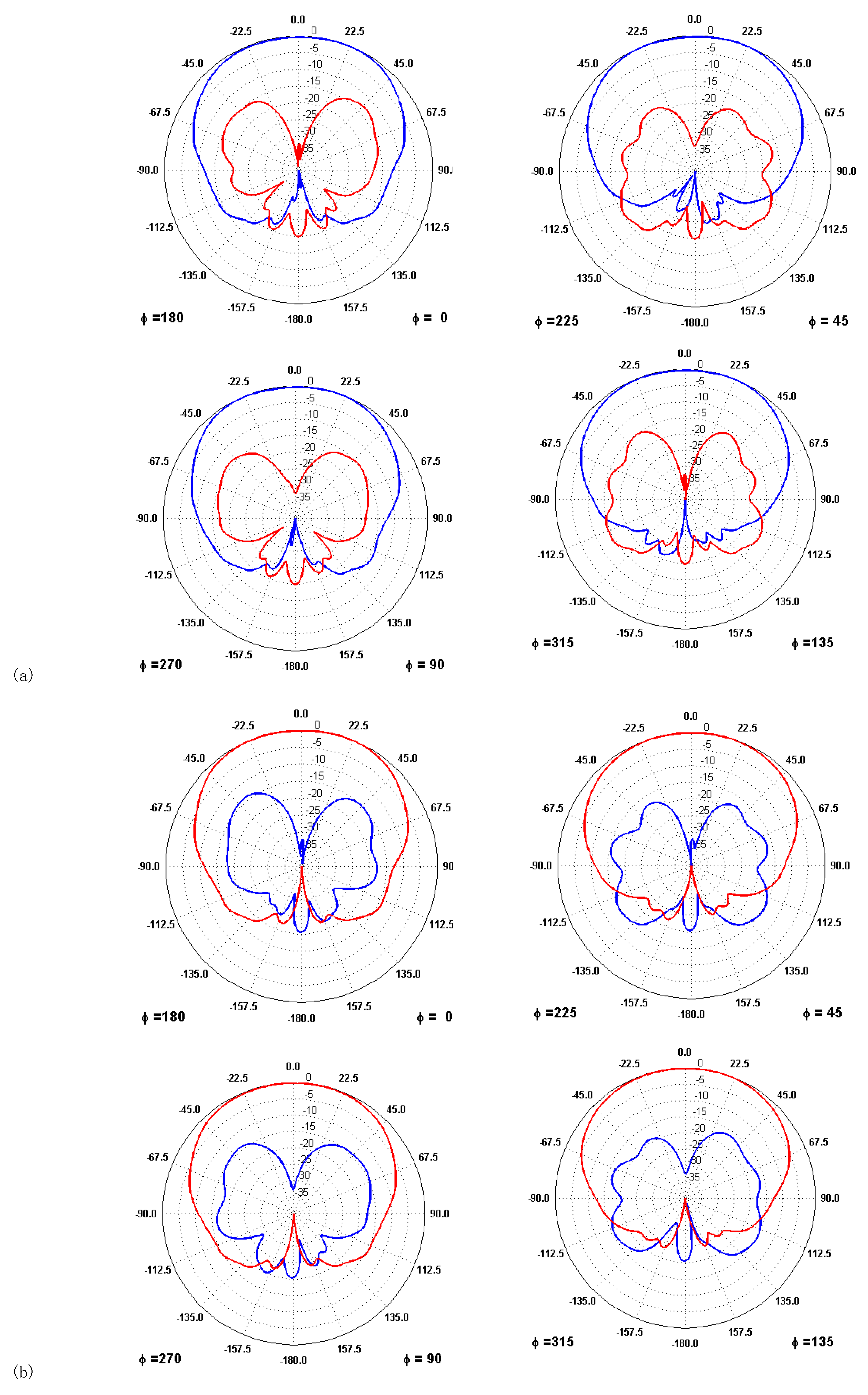
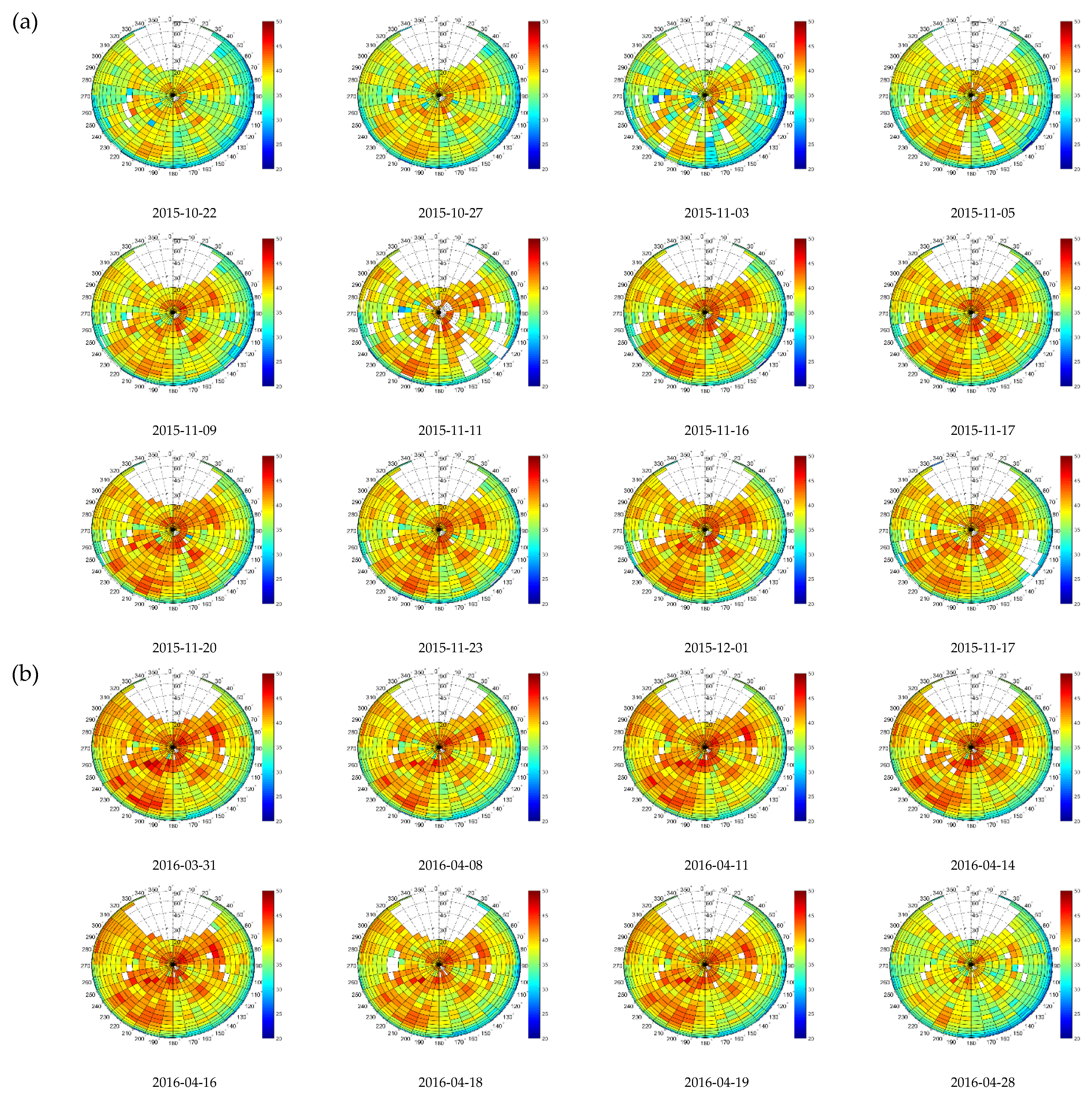
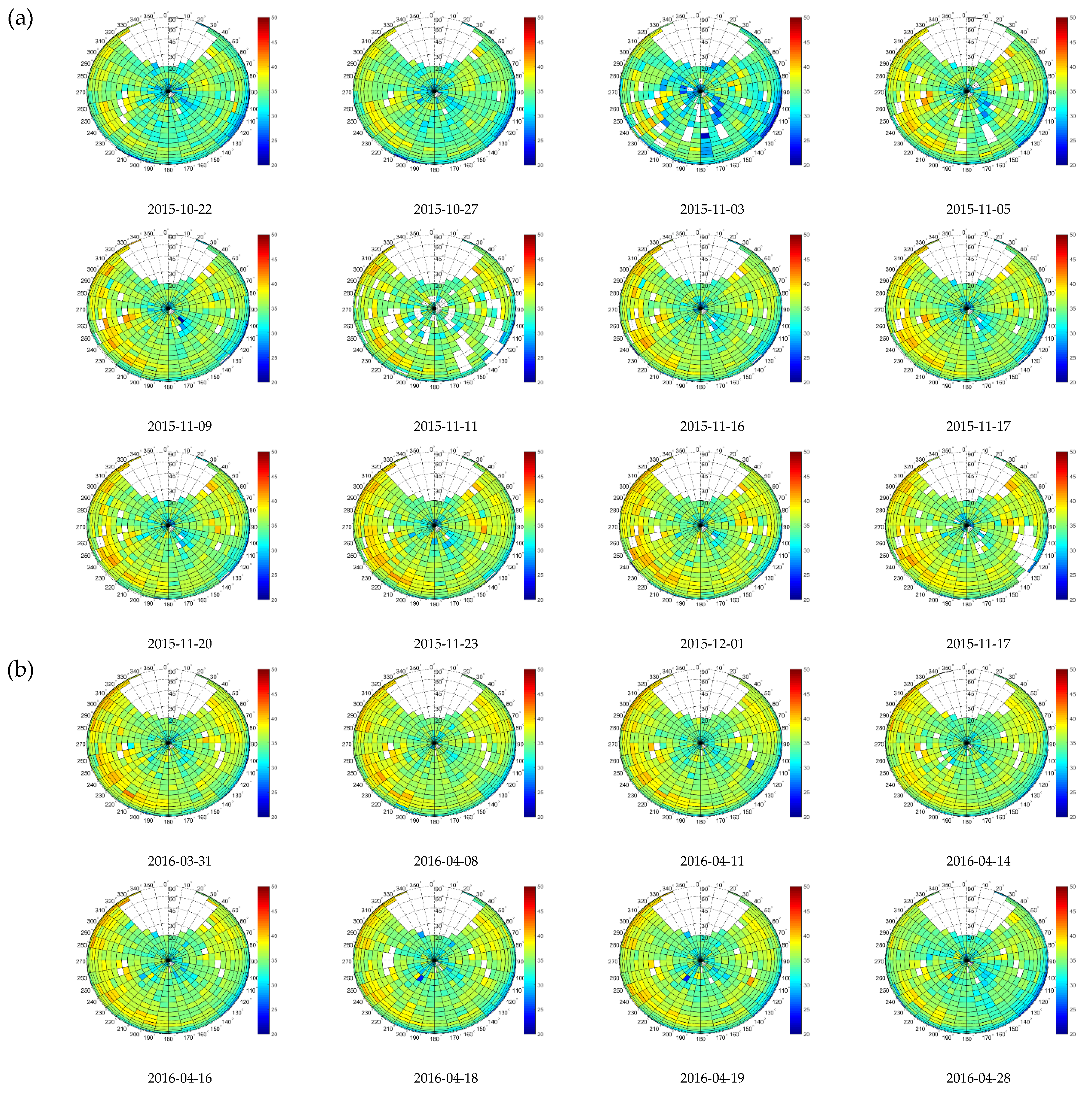
Figure 6 and Figure 7 show polar plots of the received C/N₀ values for the RHCP and LHCP channels, respectively. During the fall seasons, it is clearly seen in the RHCP plot in Figure 6a that the smaller the number of leaves, the smaller the attenuation is. Accordingly, the C/N₀ is measured as being higher in December than in October. Leaves also cause depolarization of the waves, but from the two effects (attenuation and scattering), attenuation is dominant since the LHCP received power actually increases after the leaves have fallen, as shown in Figure 7a. Figure 6b and Figure 7b show different examples of the received C/N₀ when the leaves are growing in spring. The decrease in the received power shows again that the attenuation effect is dominant for leaves.

In the following, the received RHCP C/N₀ is azimuthally averaged to analyze the evolution with the elevation/incidence angle. Resulting C/N₀ curves are analyzed with respect to:

• rain rates, obtained from the regional meteorological station,
• blueness, greenness, redness, and sky cover percentage computed from the RGB and gray scale pictures (Figure 5),
• LAI and NDVI, both computed from MODIS,

To investigate which parameter estimates best the vegetation effects in the signal propagation.

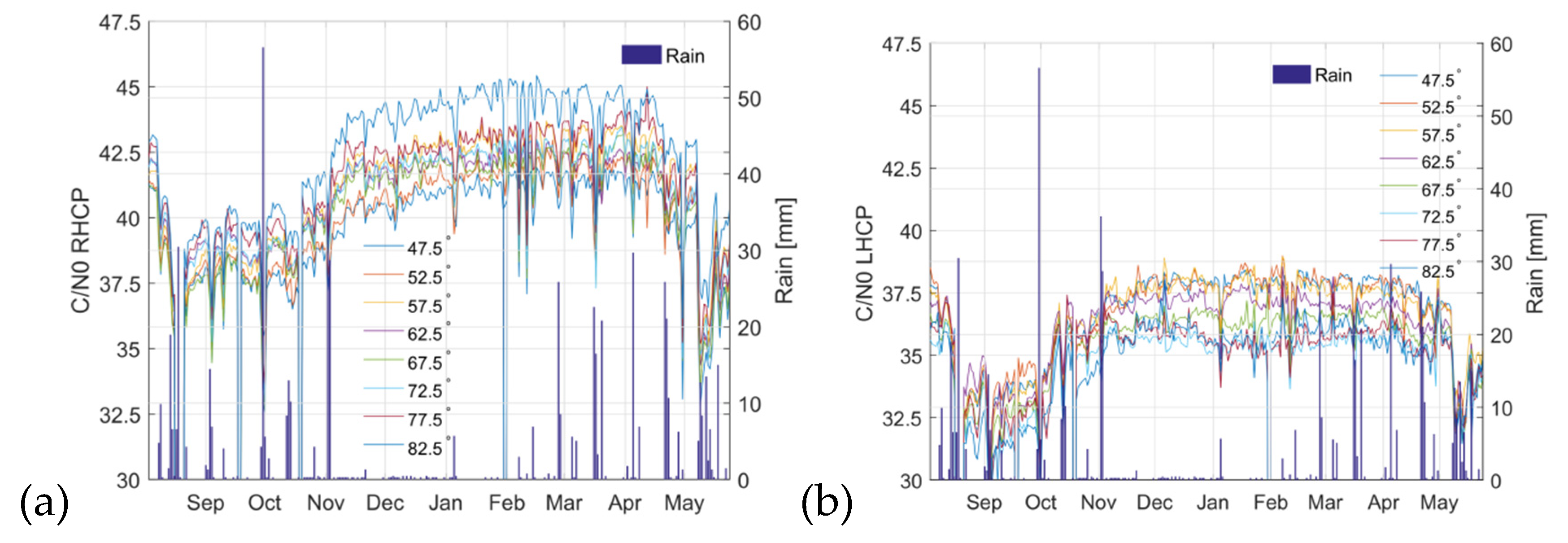
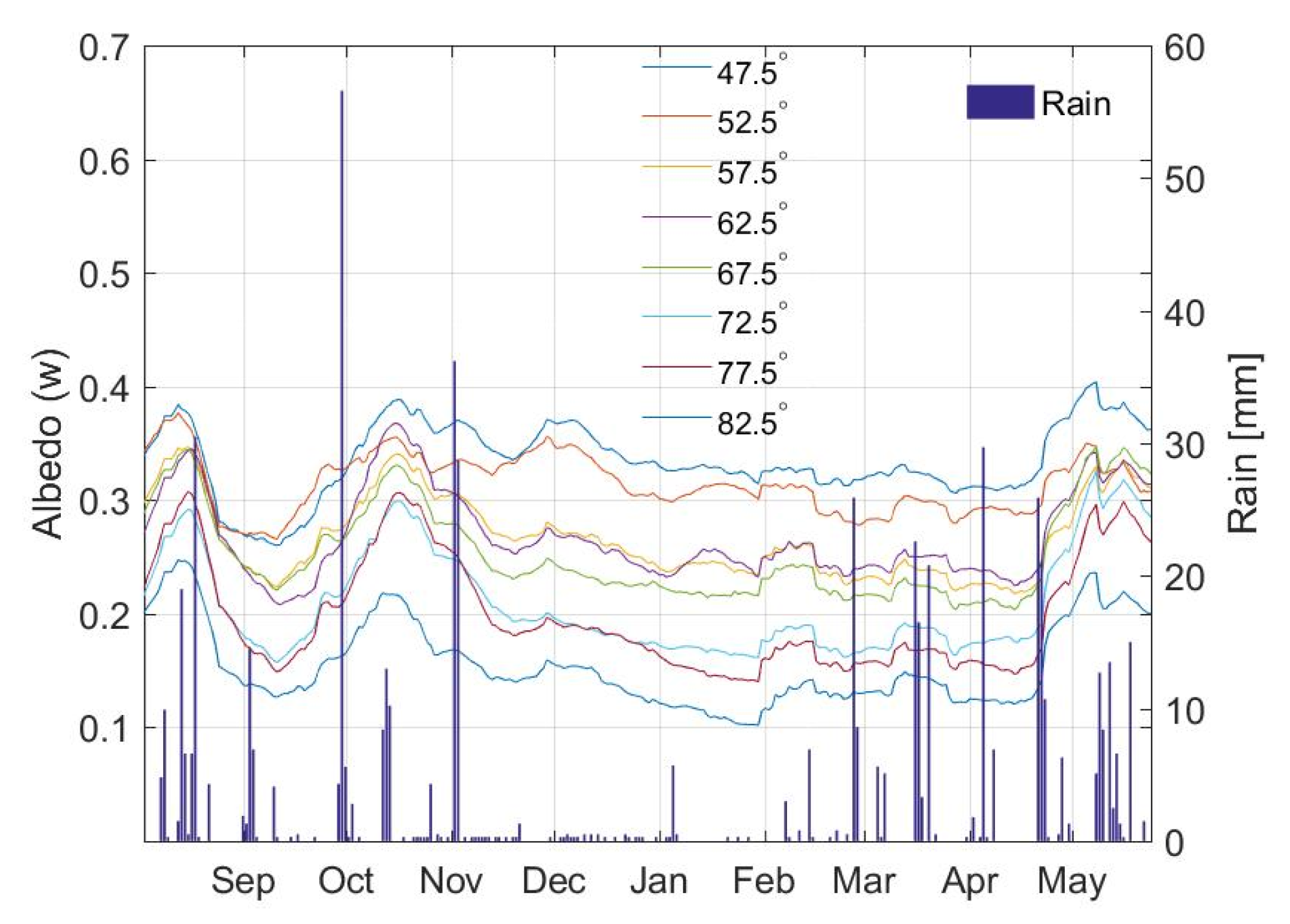
3.1. Rain Effects

Figure 8 shows the azimuthally averaged RHCP and LHCP C/N₀ curves for different satellite elevation angles as a function of time, together with the rain events during the field campaign. It can be appreciated that rain events induce a fading on the C/N₀ plots, especially in the RHCP channel, due to two main factors: (1) the presence of water drops in the atmosphere, and the water that stays on the leaves’ surface, increasing the attenuation induced by the leaves; (2) the fact that after the rain event, trees absorb the water from the soil, increasing the vegetation water content. Note that during the period without leaves (December 2015–April 2016), fading events due to rain are very smaller in depth.

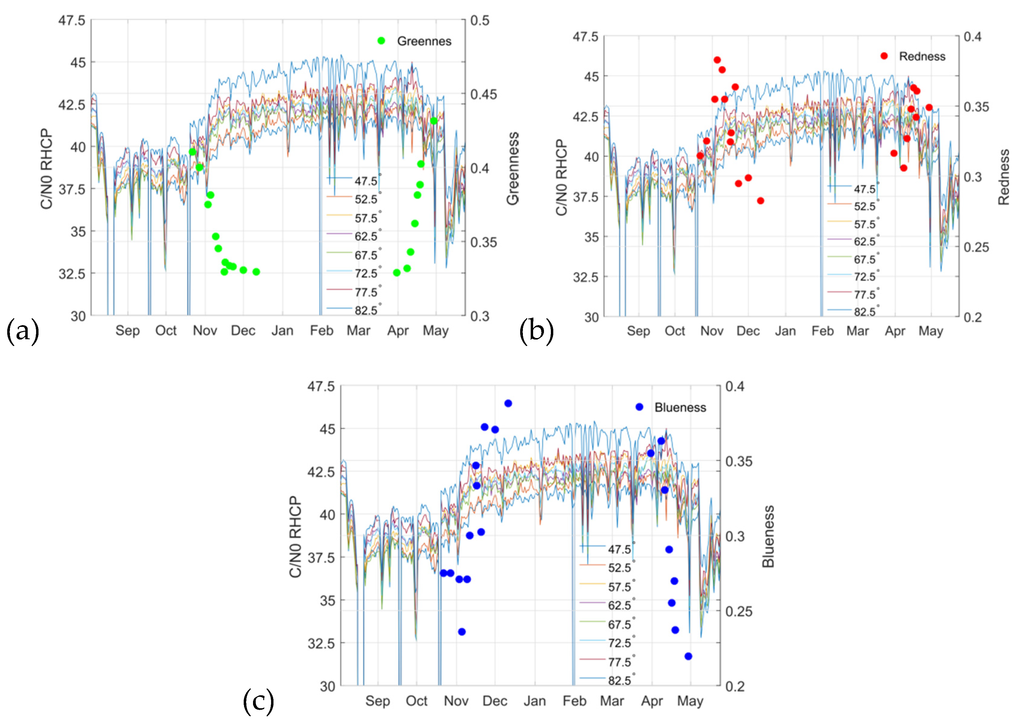
3.2. Dependence on the Greenness/Redness/Blueness

The greenness, redness, and blueness can be estimated from the color histograms as:

$$G,R,B=\frac{{\rho }_{G,R,B}}{{\rho }_G+{\rho }_R+{\rho }_B},$$

(1)

where ρ_G,R,B is the amount of G,R,B color bits from the pictures taken with the Canon 50-D. Figure 9a shows the evolution of the greenness estimated from the pictures together with the azimuthally averaged RHCP C/N₀ curves. It is expected that the larger the greenness parameter, the larger the amount of leaves, and therefore the larger the attenuation. During the defoliation process (October–December 2015), the R² parameter with a linear fit computed between the greenness and the different C/N₀ curves is 0.76–0.87; it does not depend on the incidence angle, and the mean slope of the fit is −31 dB/au (au: arbitrary unit). During the leaf growing period (March–April 2016), the R² parameter goes down to 0.46–0.66.

Figure 9b shows the RHCP C/N₀ curves together with the redness parameter. The R² parameter for both the falling and growing season is below 0.05 for any elevation angle, and it does not depend on the season.

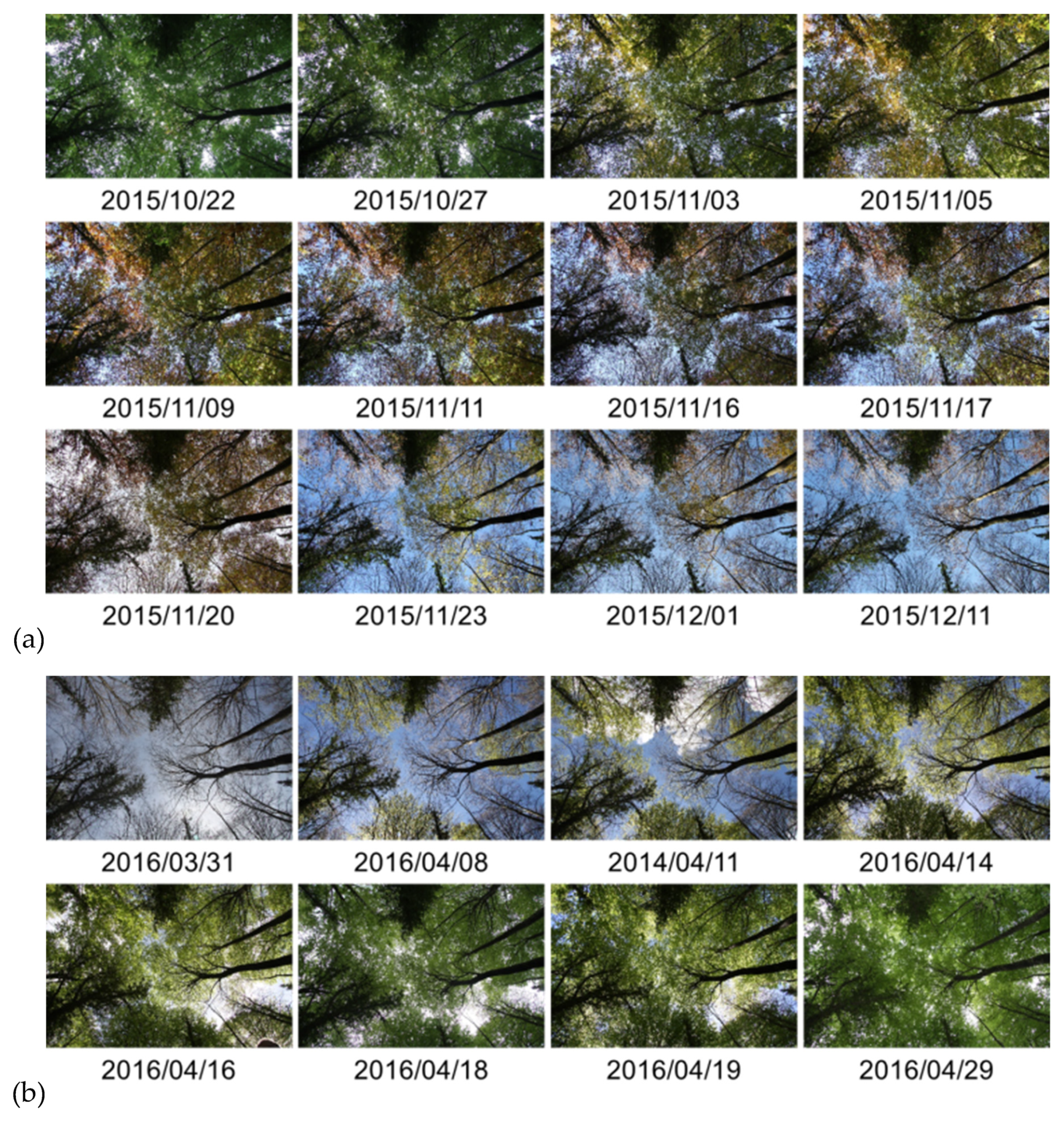
Finally, Figure 9c shows the RHCP C/N₀ curves together with the blueness parameter. As for the greenness parameter, C/N₀ curves and blueness are correlated, but not as correlated as with the greenness. During the defoliation process, R² is ~0.46–0.58 with a slope of ~14 dB/au, while during the growing process, R² is ~0.25–0.43, with a slope of 10 dB/au. The correlation between curves appears because the amount of blue is related to the amount of sky observed, and therefore the larger the amount of sky observed, the lower the amount of leaves; however, the amount of blue color seems to be a poor vegetation indicator. Apart from that, on a cloudy day, such as 2015/11/20 or 2016/03/31, the sky is white and not blue (see Figure 4), and therefore the blueness is not such a good indicator.

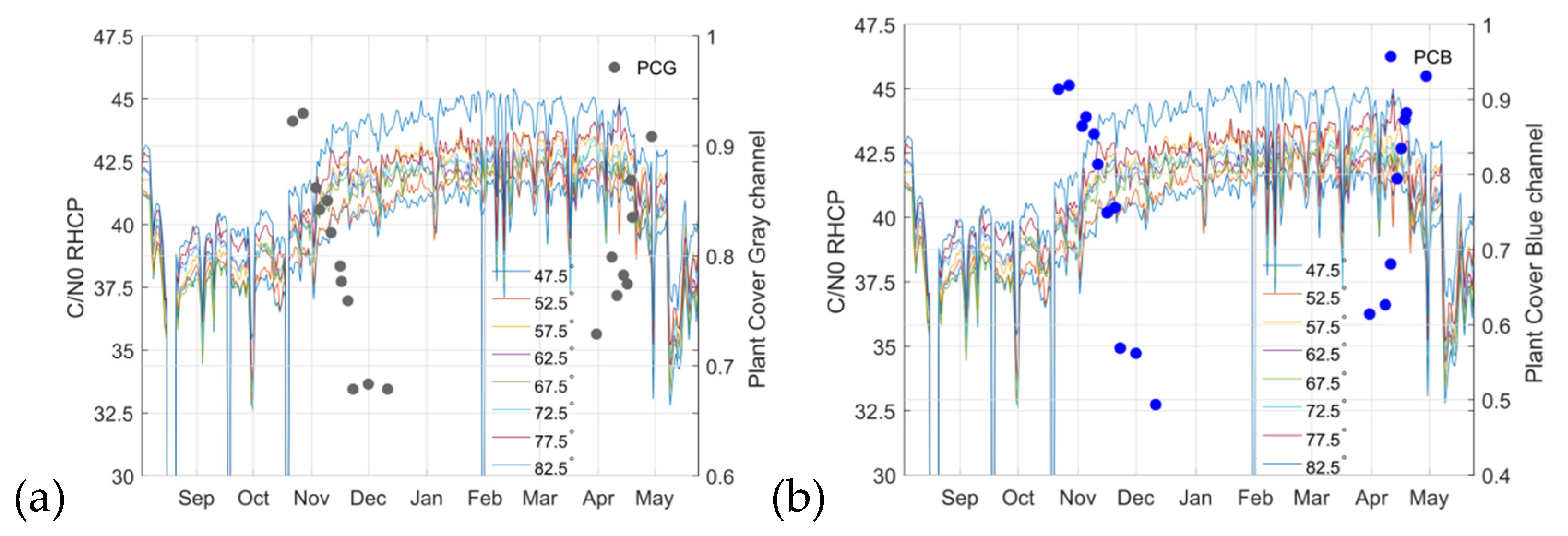
3.3. Dependence on the Sky Cover

Figure 10 shows the RHCP C/N₀ curves together with the fraction of sky covered computed in two different ways. In Figure 10a, it is computed from the gray-scale image (intensity, 0–255). A value threshold of 155 is selected [8,9] to differentiate between the vegetation (vegetation < 155), and the sky (open sky > 155). In Figure 10b, the blue channel of the RGB image is used for sky classification, and a similar threshold is applied.

Regarding the percentage of sky cover computed from the gray-scale image, the R² parameter with a linear fit between the different C/N₀ curves and the percentage of sky cover is 0.6–0.7 for the falling season, whereas it is between 0.67 and 0.82 for the growing season. However, when using the blue channel to estimate the percentage of sky cover, the R² parameter is between 0.47 and 0.57 for the fall season, and 0.3 and 0.5 for the spring season. Again, both are independent of the elevation angle.

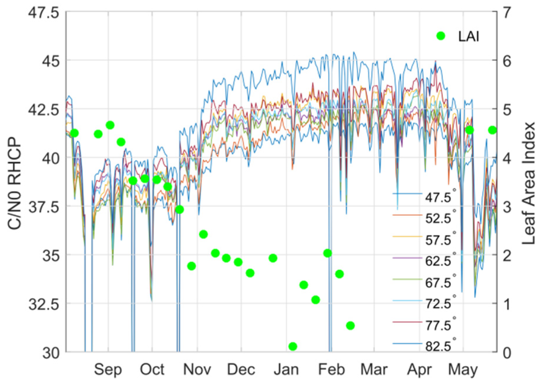
3.4. Dependence on the LAI

Figure 11 shows the evolution of the LAI parameter and the RHCP C/N₀ curves for different elevation angles. The R² coefficient of the regression lines that relate the RHCP C/N₀ to the LAI ranges from 0.50 and 0.62, which is still lower than the greenness parameter. However, a trend can be clearly seen in Figure 11 where the lower the LAI, the larger the C/N₀ observed.

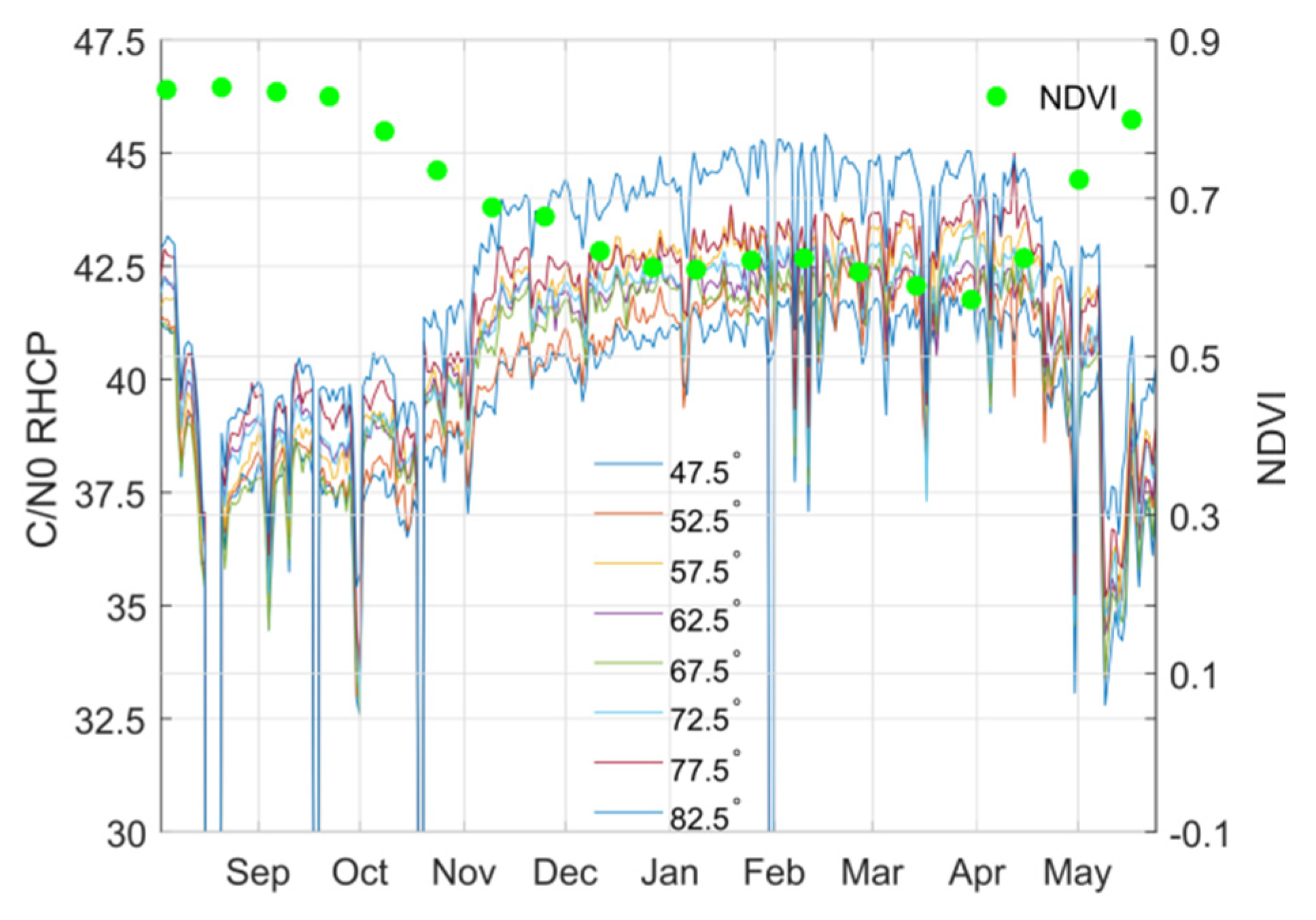
3.5. Dependence on NDVI

Figure 12 shows the evolution of the NDVI parameter and the RHCP C/N₀ curves for different elevation angles. There is a very high correlation between the received signal power or C/N₀ and the NDVI.

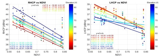
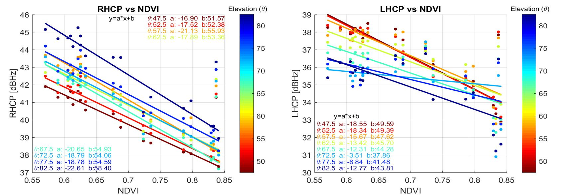
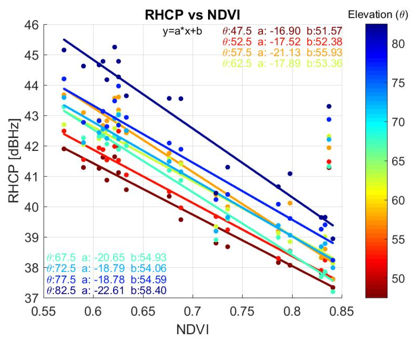
Figure 13 compares the NDVI values against the mean C/N₀ value for different satellite elevation angles. For all satellites and elevation angles the R² parameter is between 0.87 and 0.94, and the slope of the fit from −16.9 dB/au to −22.6 dB/au (au denotes an arbitrary unit of the NDVI from 0 to 1).

Table 1. RHCP C/N₀ vs. NDVI fitting parameters.

	RHCP
Elevation Angle [deg]	a [dB/au]	b [dB]	RMSE [dB]	R2
47.5	−16.90	51.57	0.55	0.89
52.5	−17.52	52.38	0.49	0.92
57.5	−21.13	55.93	0.61	0.91
62.5	−17.89	53.36	0.65	0.86
67.5	−20.65	54.93	0.48	0.94
72.5	−18.79	54.06	0.62	0.89
77.5	−18.78	54.59	0.66	0.88
82.5	−22.61	58.40	0.71	0.90

(y = a·NDVI + b, RMSE: root mean square error, and coefficient of determination R²).

(columns 2 to 5) shows the fitting parameters of the regression of the RHCP C/N₀ with respect to NDVI as a function of the elevation angle (Figure 13).

4. Discussion

From all the previous analysis, it can be concluded that the NDVI is the best descriptor to account for the vegetation attenuation for the forest type of our experiment. This parameter will now be used in our discussion on the signal depolarization through the vegetation.

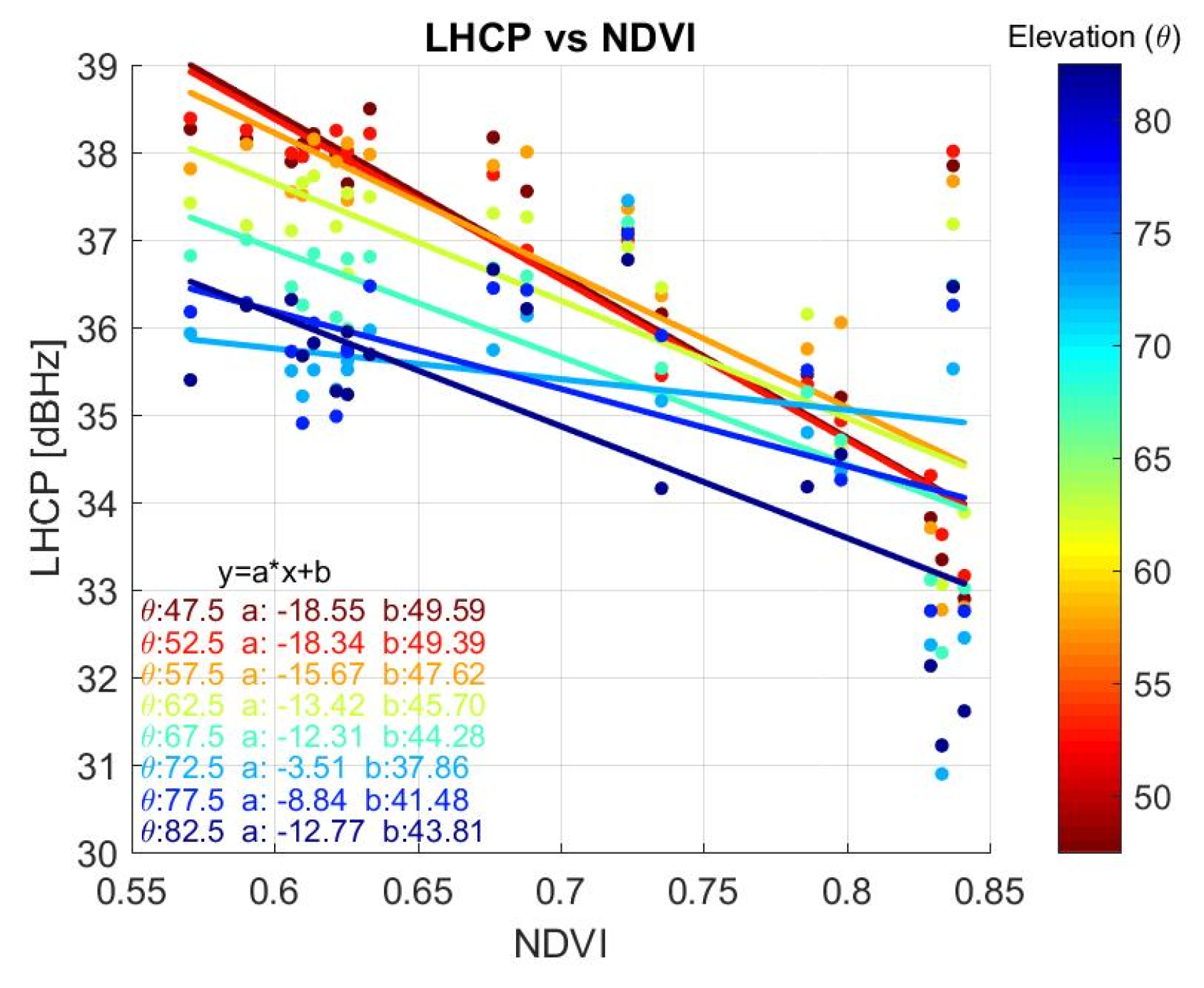
The dependence between the LHCP C/N₀ and the NDVI (Figure 14) is also found to be strongly correlated. Because of the increased attenuation, the larger the NDVI, the lower the received power at LHCP.

Table 2. RHCP and LHCP C/N₀, and Co- to Cross-polar Ratio vs. NDVI Fitting Parameters.

	LHCP				RHCP to LHCP Ratio
Elevation Angle [deg]	a [dB/au]	b [dB]	RMSE [dB]	R2	a [dB/au]	b [dB]	RMSE [dB]	R2
47.5	−18.55	49.59	0.80	0.82	1.65	1.98	0.97	0.86
52.5	−18.34	49.39	0.62	0.88	0.82	2.99	0.79	0.73
57.5	−15.67	47.62	1.09	0.65	−5.46	8.31	1.25	0.59
62.5	−13.42	45.70	0.96	0.63	−4.47	7.66	1.16	0.54
67.5	−12.31	44.28	0.98	0.59	−8.34	10.65	1.09	0.55
72.5	−3.51	37.86	0.79	0.76	−15.28	16.20	1.00	0.68
77.5	−8.84	41.48	1.31	0.31	−9.94	13.11	1.47	0.27
82.5	−12.77	43.81	1.31	0.43	−9.90	14.59	1.49	0.39

(y = a·NDVI + b, RMSE: root mean square error, and coefficient of determination R²).

(columns 2 to 5) shows the fitting parameters of the regression of the LHCP C/N₀ wrt. NDVI as a function of the elevation angle (Figure 14).

However, it must be noted that:

• The correlation drops at high elevation angles (77.5° and 82.5°) because the path through the vegetation layer is shorter, and scattering effects (responsible for signal depolarization) are less important.
• The slope is (in absolute value) smaller for LHCP than for RHCP, suggesting a combined effect of depolarization that transfers power from the RHCP signal to the LHCP.

The ratio LHCP/RHCP vs NDVI (Figure 13 minus Figure 14 in dB) also exhibits an interesting behavior. At mid-low elevation angles, the dependence on the vegetation is small (small slope) and the independent coefficient b is also very small, indicating that the incoming RHCP wave is almost completely depolarized. As the elevation angle increases, the absolute value of the slope (a) and the independent coefficient (b) both increase (Table 2, columns 6 and 7). These results are in agreement with [10], showing how the polarization ratio of the GNSS-R observables decreased with increasing vegetation, in [10] parametrized with the Leaf Area Index.

These results also indicate that, as pointed out in [11], a correction based on the compensation of the (two-way) vegetation optical depth is not appropriate and a more refined vegetation model that properly accounts for vegetation scattering must be used in soil moisture retrieval algorithms using GNSS-Reflectometry.

In an attempt to refine the inclusion of vegetation effects, a more refined τ-ω model is proposed, with variable parameters with the elevation angle. By fitting the observed data to a simple τ-ω model, an albedo (ω(θ_e)) value can be estimated. Figure 15 shows the evolution of the estimated albedo with respect to time for several elevation angles. As it can be appreciated, there is a strong dependence with the elevation angle, and apparently a weak dependence with the NDVI (not shown in this plot, but NDVI varies from 0.6 to 0.9, see Figure 12). Figure 16 shows the regression lines of the albedo with respect to NDVI for different elevation angles, and

Table 3. ω vs. NDVI Fitting Parameters.

Elevation Angle	a [-]	b [-]	RMSE [-]	R2
47.5	−0.08	0.38	0.05	−0.17
52.5	−0.02	0.32	0.03	−0.20
57.5	0.16	0.14	0.04	0.05
62.5	0.10	0.18	0.04	0.05
67.5 *	0.26	0.06	0.04	0.52
72.5 *	0.17	0.07	0.05	0.46
77.5	0.22	0.03	0.05	0.19
82.5 *	0.21	0.00	0.03	0.66

Note: Only elevation angles marked with an “*” are significant (R² > 0.4).

shows the fit parameters of Figure 15. The albedo varies from ~0.1 to 0.2 at the zenith, but up to ~0.35 at 47.5°. Note, however, that only at high elevation angles (θ_e≥ 67.5°) is the single scattering albedo correlated with the NDVI, and at lower elevation angles, the presence of multiple scattering makes the τ-ω model more likely to be invalid.

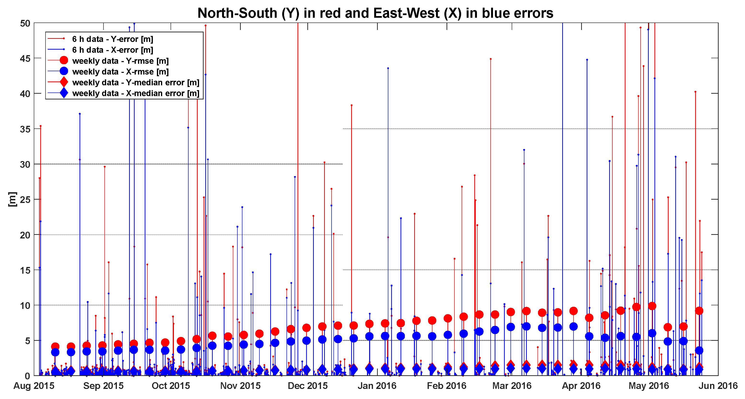
As a side parameter, Figure 17 shows the evolution of the 6-h position error (stem plot), the weekly root man squared errors (circles), and the median errors (diamonds) in north-south (Y-component, in red) and east-west (X-component, in blue). In general, the error increases over time, from August 2015 to the end of May 2016. In general, the increase in spring can be due to extra attenuation due to the water content in the leaves (Figure 12). However, there is a sudden NDVI increase in mid-April that translates into a smaller positioning error. Additionally, the smaller rmse and monotonic increase in the late summer and early fall cannot be explained by the NDVI (Figure 12); as leaves get drier and finally fall, the attenuation also decreases, and so the NDVI slowly decreases in October until mid-November. Here, the only plausible explanation encountered would be the increased scattering in the tree branches that creates a multipath, which is then reduced as leaves appear and attenuate the signal, but also the multiple-scattering (multi-path) as well. This empirical result turns out to be in very good agreement with Figure 4, left, where Zimbelman et al. [12], predicted a 10 m rmse error for 20 m tall trees, as the ones shown in Figure 5.

5. Summary and Conclusions

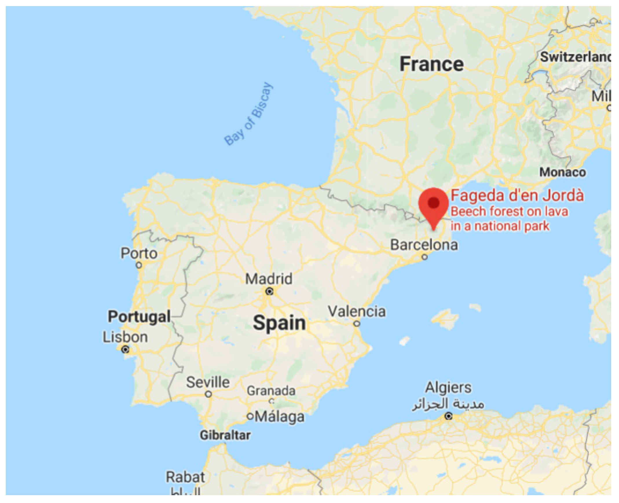
A one year long field experiment was conducted between 8/2015 and 10/2016 at La Fageda d’en Jordà forest in the north east of Spain, to assess the vegetation impact on the propagation of GNSS signals, as this is a critical correction for the accurate soil moisture retrieval using GNSS-Reflectometry.

The correlation of the vegetation co-polar (RHCP) attenuation has been evaluated against different vegetation descriptors, such as the rain, the greenness, blueness and redness indices, the sky cover, the LAI, and the NDVI. It has been found that among all of them, the correlation with the NDVI shows the highest R² parameter (>0.85), with sensitivities ranging from −17 dB/au to −23 dB/au. This indicates that at L-band, auxiliary NDVI data can be used as a descriptor for beech forest vegetation attenuation in GNSS-R soil moisture retrievals. Alternatively, L-band multi-angular attenuation measurements can be used to infer the vegetation water content, which is related to the vegetation optical depth (VOD).

The correlation of the vegetation cross-polar (LHCP) attenuation with the NDVI has also been evaluated, finding lower values (~0.55), but still significant. The LHCP signal is ~9 dB to ~3 dB below the RHCP signal around zenith and elevation angles of 82.5° and 47.5°, respectively. This indicates that the lower the elevation angle, but even as high as 47.5°, the more important the multiple scattering effects are, and so the signal depolarization.

Trying to find an equivalent “single scattering albedo” (ω) dependent on the elevation angle, that could be used in a τ-ω model, it was found that it varies from ~0.1 to 0.2 at the zenith, and increases up to ~0.35 at 47.5°. However, only at high elevation angles (θ_e≥ 67.5°), the estimated albedo is significant, and can be related to the NDVI. At lower elevation angles, signal depolarization and multiple scattering effects must be taken into account to properly model vegetation effects in GNSS-Reflectometry, for this type of forest, and probably for other types of dense vegetation as well. This limitation of the model is what nowadays limits the range of elevation angles that can be used for soil moisture retrievals using GNSS-R, as shown in [13].

Finally, the evolution of the rmse positioning error is shown wrt time, which exhibits an increase from 3–4 to 6–10 m from fall to late spring, as shown in [12].