Estimating Near Real-Time Hourly Evapotranspiration Using Numerical Weather Prediction Model Output and GOES Remote Sensing Data in Iowa

Abstract

This study evaluates the applicability of numerical weather prediction output supplemented with remote sensing data for near real-time operational estimation of hourly evapotranspiration (ET). Rapid Refresh (RAP) and High-Resolution Rapid Refresh (HRRR) systems were selected to provide forcing data for a Penman-Monteith model to calculate the Actual Evapotranspiration (AET) over Iowa. To investigate how the satellite-based remotely sensed net radiation ($R_n$) estimates might potentially improve AET estimates, Geostationary Operational Environmental Satellite derived $R_n$ (GOES-$R_n$) data were incorporated into each dataset for comparison with the RAP and HRRR $R_n$-based AET evaluations. The authors formulated a total of four AET models—RAP, HRRR, RAP-GOES, HRRR-GOES, and validated the respective ET estimates against two eddy covariance tower measurements from central Iowa. The implementation of HRRR-GOES for AET estimates showed the best results among the four models. The HRRR-GOES model improved statistical results, yielding a correlation coefficient of 0.8, a root mean square error (mm hr⁻¹) of 0.08, and a mean bias (mm hr⁻¹) of 0.02 while the HRRR only model results were 0.64, 0.09, and 0.04, respectively. Despite limited in situ observational data to fully test a proposed AET estimation, the HRRR-GOES model clearly showed potential utility as a tool to predict AET at a regional scale with high spatio-temporal resolution.

1. Introduction

1.1. Importance of Evapotranspiration

Actual evapotranspiration is a key element of the land-surface water and energy cycle, strongly influencing the distribution of water and energy exchanges between the surface and atmosphere [1,2,3]. Understanding evapotranspiration is important in managing water resources such as irrigation scheduling. Accurately predicting AET also is important for regional weather and global climate model predictions, as AET is tightly linked to hydrological and climate processes such as precipitation, runoff, and air temperatures close to the surface and in the Atmospheric Boundary Layer (ABL) [4,5,6,7,8,9,10].

Globally, the amount of water lost to the atmosphere through ET is approximately 60% of annual land precipitation [11]. In arid areas, AET can transfer more than 90% of annual precipitation to the atmosphere [12]. AET is the second highest element of the water budget in the global hydrologic cycle after precipitation, except in tropical areas [13]. Moreover, AET influences precipitation amounts from the land surface and available surface energy [14]. Reliable estimates of AET are essential for hydrologic and climate prediction to improve flood forecasting, drought detection, and risk assessment [15,16,17], and to determine reservoir losses and agricultural water management [18].

1.2. Background

1.2.1. In Situ AET Measurements and Their Limitations

AET can be measured most directly using weighing lysimeters [19]. It also can be estimated in situ using Bowen ratio methods [20] or Eddy Covariance (EC) methods [21] or evaluated as a residual term in surface energy/water balance equations [22]. Measuring or estimating AET by these methods is not a commonly practiced or easy task, especially over regional or larger scales. Such in situ measurements are very challenging, as they involve high labor costs and require high-precision instrumentation, especially with lysimeter and EC systems [23,24]. Over regional scales, AET estimation has been a challenge because surface observations of AET are typically only available on field scales. For this reason, Remote Sensing (RS) data are often used to provide data for AET estimates on regional to global scales, since such methods can provide cost-effective spatially distributed data [25,26].

1.2.2. AET Estimates Using Remote Sensing Techniques

This study concentrates on satellite-based RS methods. Such RS techniques are suitable to continuously monitor land surface properties over wide areas [27] and RS products also can provide a useful tool for detection and mitigation of natural disasters such as flooding, fires, hazardous weather conditions, and volcanoes by surveying areas inaccessible with in situ methods [28].

However, RS products often require substantial processing time and supplementary data to produce and distribute the final AET estimates. Some satellite platforms have longer revisiting times (e.g., 16 days for LANDSAT and ASTER versus one day for MODIS and half-hourly for GOES), although satellites with longer revisiting times often provide a finer spatial resolution (e.g., near or less than 100 m from LANDSAT and ASTER depending on channels versus 1 km from MODIS). Such trade-offs between spatial and temporal resolutions are a potential issue for AET estimation at shorter time scales and over regional scales. To obtain input data for near real-time operational AET estimates on this scale with our criteria of a short product lag time (<a few hours), moderate but not too coarse spatial resolution (<20 km), and a high temporal resolution (<1 day), we investigated methods to use numerical weather prediction (NWP) output data as forcing for regional-scale AET estimates. The aim of this strategy is to overcome some of the shortcomings that other field and RS data might exhibit regarding an operational real-time AET assessment.

Deriving net radiation ($R_n$) for regional-scale AET estimation using RS data-based models such as SEBAL, METRIC, and ALEXI [16,29,30,31] requires land surface temperature (LST) data from thermal infrared (TIR) satellite channels. Several remote sensing AET methods also use LSTs or their time change to evaluate the thermodynamic state of the surface and/or ABL and the surface energy balance, including AET. LST estimates from satellites require cloud-free observation conditions, and thus easily can be contaminated by an undiagnosed small-scale cloudiness in the satellite images [32,33]. Deriving LST values also requires detailed knowledge of the atmosphere between satellite and ground target to adjust Top-of-Atmosphere (TOA) satellite TIR radiance measurements to represent the surface radiative temperature [34].

Given the complexities in obtaining LST values from satellite data and the considerable data burden, hourly estimated meteorological data from the NWP output may be a useful alternative, especially in agricultural regions, where LST values are not typically much higher than shelter-level air temperatures or forecast model predictions of air temperature.

Although we did not use TIR RS data as input data for $R_n$ and subsequent AET estimates, GOES insolation data have been used successfully in several studies to estimate $R_n$ and AET in agricultural environments [35,36]. There is also some precedent for the combination of GOES cloud/insolation data with NWP outputs. In this study, we describe how satellite-based RS $R_n$ data derived from the GOES insolation product improved AET estimates from the National Oceanic and Atmospheric Administration’s National Center for Environmental Prediction (NOAA/NCEP) Rapid Refresh (RAP) and High-Resolution Rapid Refresh (HRRR) $R_n$-based outputs under certain situations. These are investigative areas that to date have not been well studied. Note that the HRRR uses remote sensing data from ground-based (weather radar) and satellite platforms. Radar reflectivity as well as atmospheric motion vectors are just a few relevant examples. However, our emphasis is on the value of GOES insolation.

1.2.3. Models Providing AET Estimates or Variables to Estimate AET

Several models continuously provide either AET datasets or surface forcing data that can be used to estimate regional-scale AET. The three models detailed below generate AET and products that can be used to estimate AET with varying temporal and spatial resolutions within the model forecasts.

The North American Land Data Assimilation System (NLDAS) is a collaborative project that provides continuous data over the Coterminous United States (CONUS) to supply initial conditions for NWP [37,38]. The NLDAS provides hourly AET data with a 0.125° (approximately 13 km) spatial resolution using four land-surface models: Mosaic, Noah, Sacramento Soil Moisture Accounting (SAC-SMA), and Variable Infiltration Capacity model (VIC). There are eight surface meteorological variables in the NLDAS: 2 m air temperature (K) and specific humidity (kg kg⁻¹); incoming short- and long-wave radiation (W m⁻²); 10 m zonal and meridional wind speeds (m s⁻¹); surface pressure (kPa); and hourly integrated precipitation (kg m⁻²) [39].

The Weather Research and Forecasting (WRF) model hydrological extension package (WRF-Hydro) was developed at the National Center for Atmospheric Research (NCAR) to couple hydrological and atmospheric models with earth system models. Outputs of WRF-Hydro include surface soil evaporation (mm) and transpiration (mm); surface latent heat; surface sensible heat and ground heat fluxes (W m⁻²); soil moisture (m³ m⁻³) and temperature (K); and other related quantities [40]. The WRF system uses the NOAA/NCEP Global Forecasting System (GFS) to build initial and boundary conditions for the forecast simulations. Four horizontal resolution values (approximately 18, 9, 3, and 1 km) are available through the WRF system [41].

The Noah-MP LSM (Noah land surface model with multi-parameterization) is a research community effort to improve the Noah LSM by implementing more realistic hydrological and surface energy exchange processes [42]. It is supported within the WRF-Hydro [40]. To implement multi-parameterization processes through the Noah-MP LSM, the canopy surface is separated from the ground surface to provide realistic heterogeneity in the land surface character [42]. ET is represented as a latent heat flux from (1) evaporation of the canopy-intercepted water and from the vegetated or non-vegetated ground, and (2) transpiration through plant stomata.

1.3. Motivation and Goals of the Current Study

Our motivation for this study is to improve the real-time operational streamflow and flood forecasting by the Iowa Flood Center (IFC) [43]. The IFC operates a detailed distributed hydrologic model called the Hillslope-Link Model (HLM) detailed in Quintero et al. [44]. The model follows landscape decomposition proposed by Mantilla and Gupta [45]. Derived from high-resolution Digital Elevation Model (DEM) data, the river network of channel links drains a system of non-overlapping hillslopes. Each link drains exactly one hillslope and hillslopes are irregular-shaped polygons.

Mathematically, the model is a system of ordinary differential equations that follow a tree-like topology. The conversion of rainfall takes place at hillslopes with partitioning into surface and subsurface runoff delivery to channel links. The partitioning has the form of a mass balance equation with rainfall and AET being the external forcings. The runoff delivered to the channels is routed using a basin-wide water velocity model [46]. The output of the model (streamflow) is updated every 15 min for some 400,000 locations within Iowa and communicated to the public via the Iowa Flood Information System (IFIS), an online interactive portal [47]. The computational efficiency of the system comes from an adaptive numerical solver detailed in small et al. [48].

The current version of HLM uses a MODIS-derived monthly ET climatology. We hope that a near real-time operational AET component would improve the existing HLM simulation results by providing AET datasets at a more frequent time interval. Therefore, the goal of this study is to evaluate NWP-based AET models (NWP-AET models) in Iowa incorporating GOES-$R_n$ data in near real-time. We used two NWP output data sets, RAP and HRRR from NOAA/NCEP. GOES-derived $R_n$ was incorporated into these model outputs to investigate how $R_n$ values from GOES would affect AET estimates. The models were validated using EC flux tower measurements. The long-term plan is to provide these hourly AET estimates to IFIS.

This paper is organized as follows: Section 2 outlines methods that include study site descriptions, the selection of the NWP models whose outputs were used to estimate AET for the Iowa domain, and radiation budgets. Section 3 describes the study results. Discussion and conclusions are presented in Section 4 and Section 5, respectively.

2. Methods

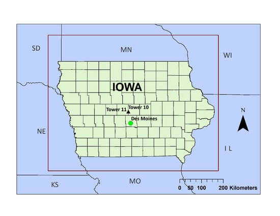
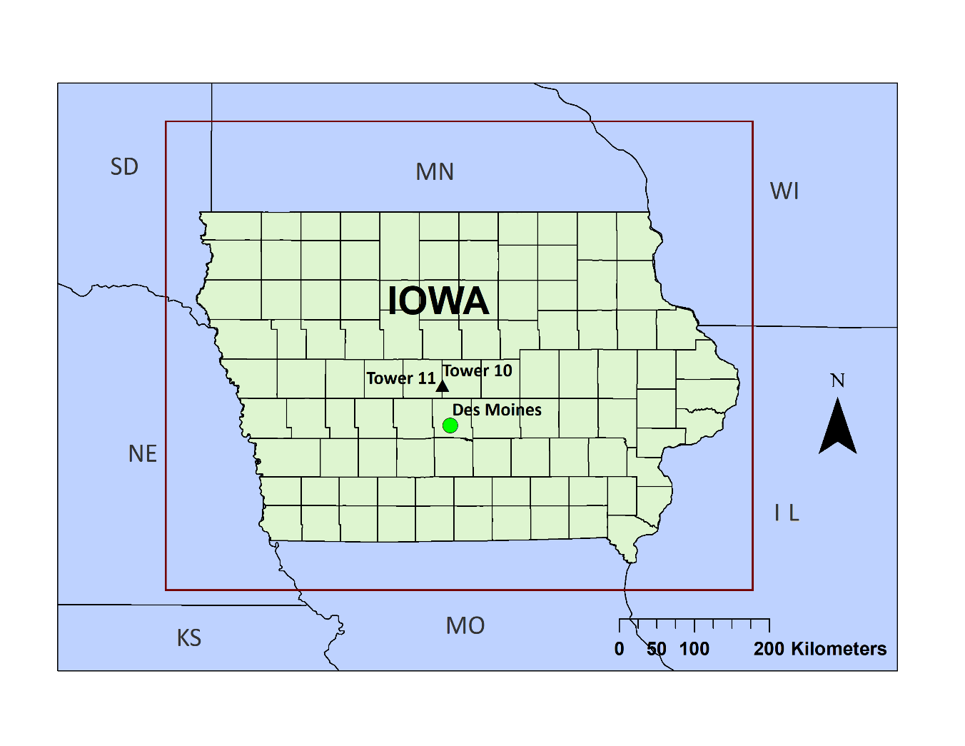
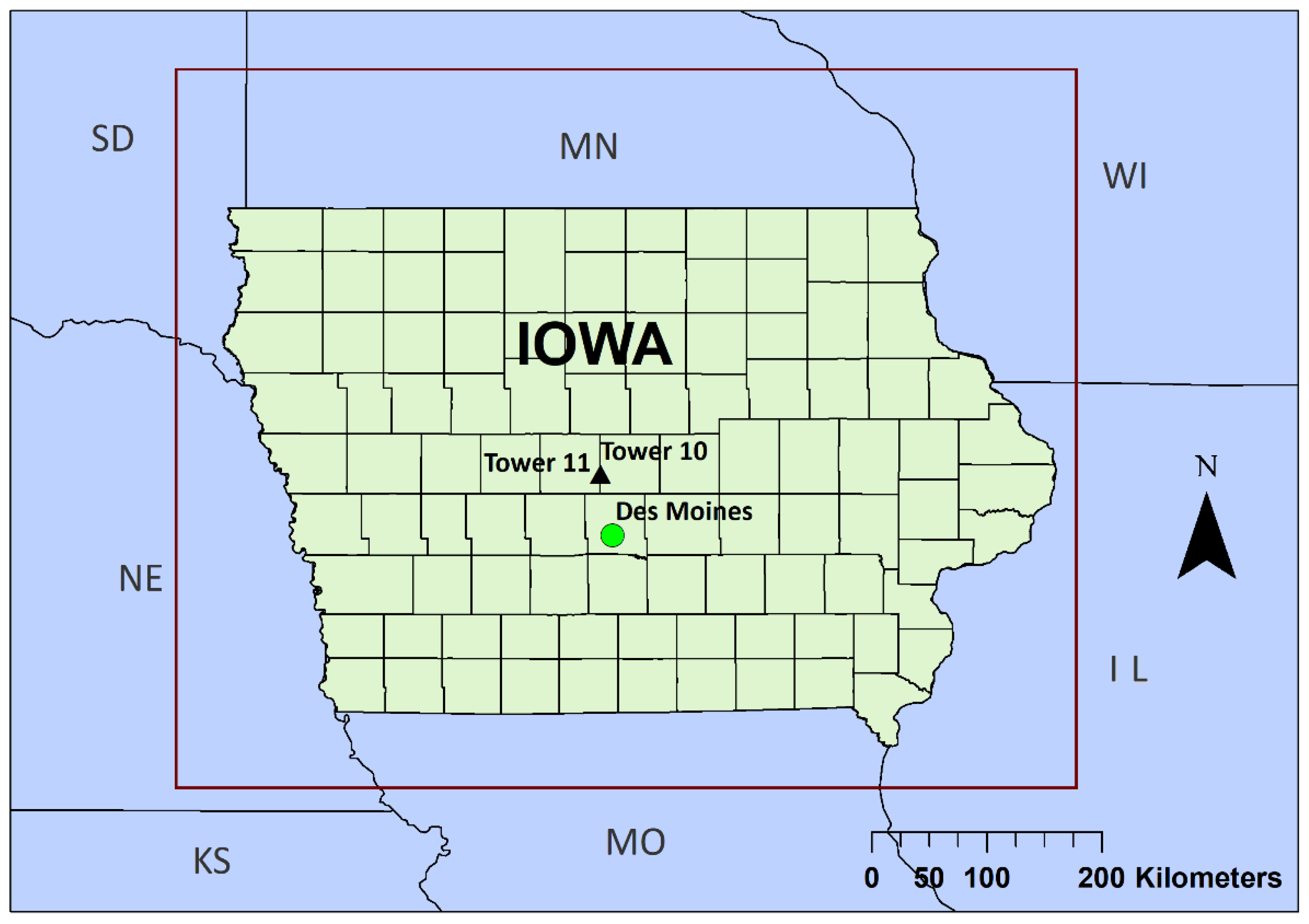
2.1. Site Description and EC Data Processing

The hydrological modeling framework that is the backbone of the IFIS [47] has a spatial domain that covers approximately 40.0 to 44.5 N and −97.0 to −90.0 W. This study domain includes the whole state of Iowa and parts of six adjacent states in the midwestern United States (Figure 1). Iowa is one of the most heavily agricultural states and is the number one state in terms of corn and soybean production [49]. Detailed information regarding the topography and landscape of Iowa can be found at the Iowa Geological Survey website [50]. The locations of the two EC towers are shown in Figure 1. The two towers are located near Ames and these towers are approximately 54 km away from the city of Des Moines. The east tower is designated Tower 10 (originally NSTL 10), while the west tower is designated Tower 11 (NSTL 11). The distance between these two towers is approximately 335 m. The tower sites are maintained and operated by the Agricultural Research Service of the United States of Department of Agriculture (USDA-ARS; formerly the National Soil Tilth Laboratory).

EC data with a 15-min averaging time were provided by the USDA-ARS in Ames, Iowa. Density variations due to the heat and water vapor transfer were considered in the calculation of latent heat flux using equations provided in Webb et al. [51]. The EC flux tower data obtained from the Tower 10 and Tower 11 sites were quality-controlled in terms of friction velocity criterion and spike detection [52]. We discarded raw EC data when the friction velocity (u^*) was smaller than the 0.1 m s⁻¹ value required to have sufficient turbulence, following the studies by Hernandez-Ramirez et al. [8,9] which used EC systems at the same locations in central Iowa as this study. Our quality control process also eliminated erroneous spikes of flux data greater than the mean plus 3.5 times the standard deviation of the values in individual datasets [10,52]. Resulting data gaps were filled using REddyProc [53]. Gap-filled 15-min averaged EC data were aggregated to hourly data for comparison with hourly modeled AET data.

To evaluate the performance of four ET models—RAP, HRRR, RAP using GOES-$R_n$ (RAP-GOES), and HRRR using GOES-$R_n$ (HRRR-GOES)—compared to the EC ET measurements, we calculated the coefficient of determination (R²), root mean square error (RMSE), mean bias (ME), mean absolute error (MAE), and Spearman correlation coefficients ($\rho$).

2.2. Selection of NWP Output Data Sets

The RAP and HRRR data are two NOAA-operated gridded numerical weather forecast outputs that produce operational hourly data analysis, assimilation, and forecast products over North America and CONUS, respectively. The RAP system has been producing data since 2012 with a spatial resolution of approximately 13 by 13 km; the HRRR system has been producing data since 2014 with a spatial resolution of 3 by 3 km. The two models generate weather forecasts and data with 21 (RAP) and 18 (HRRR) h of lead time, aiming to provide short-range weather forecasts [54].

Among the many possible regional NWP models available, we chose the RAP and HRRR products for AET estimates due to the availability of hourly outputs, which supply forcing data for AET estimates with a fine temporal resolution, adequate spatial resolution, and a relatively short lag time for availability (e.g., the model output is available a few hours after forecast model initialization). Importantly for our purposes, the RAP and HRRR outputs include variables such as incoming and outgoing short- and long-wave radiation fluxes (W m⁻²); air temperature (K); dew point temperature (K); relative humidity (%); and U- and V-components of wind speed at 10 m above ground (m s⁻¹)—all these components are necessary for the ET estimation process. Two RAP products (natural level and pressure level) and one HRRR product (surface level) have been downloaded from the NOAAs ftp sites. The desired forcing data were extracted using the wgrib2 format suggested by the Climate Prediction Center of the National Weather Service.

2.3. AET Estimates Based on the Penman-Monteith Method

The Penman-Monteith (PM) method [55], an improved version of the Penman method [56], was used to estimate potential ET (PET), incorporating the effects of the above-canopy aerodynamic resistance ($r_a$), canopy (or bulk) resistance, and stomatal resistance ($r_c$). The PM model showed the best performance in estimation of PET [36] of several models tested. The PM method is considered the standard method to estimate PET by the Food and Agriculture Organization of the United Nations [57] and the Environmental and Water Resources Institute of the American Society of Civil Engineers [58]. To calculate AET, the PET values must be adjusted to represent actual canopy and environmental conditions.

Monteith [55] presented the following equation for PET:

$$\lambda E=\frac{\Delta ·\left(R_n-G\right)+\left(\left({\rho }_a·C_p·\left(e_s-e\right)\right)/r_a\right)}{\Delta +\gamma ·\left(1+\left(r_c/r_a\right)\right)}$$

(1)

where $\lambda E$ is PET, that is, the potential canopy evaporative heat flux (W m⁻²), $\Delta$ is the derivative of the saturation vapor pressure with respect to air temperature (kPa °C⁻¹), $R_n$ is net radiation (W m⁻²), $G$ is the soil heat flux (Wm⁻²), ${\rho }_a$ is air density (kg m⁻³), $C_p$ is the specific heat of air at constant pressure (≈1013 J kg⁻¹ °C⁻¹), the $\left(e_s-e\right)$ term is the vapor pressure deficit (kPa), $r_c$ is the bulk canopy stomatal resistance (sm⁻¹), $r_a$ is the aerodynamic resistance above the canopy (s m⁻¹), and $\gamma$ is the psychrometric constant (kPa °C⁻¹).

The Crop Coefficient (Kc) method was used to convert the PM estimates of ET to AET estimates representative of Iowa crops, a method where AET is represented as PET times Kc. This Kc method was developed for well-irrigated conditions of clipped and cool-season grass or full coverage of alfalfa [58]. AET, however, needs to represent real crop conditions, not such an idealized situation. We investigated estimating AET by adjusting the calculation of Kc using the single crop coefficient approach described in Allen et al. [57], with the assumption that there are two major crops grown in Iowa—corn and soybean (60% and 40% of the total acres planted, respectively) [59]. We adopted the change of Kc values over the crop growth stage of corn and soybean depicted graphically in Allen et al. [57]. Kc values are constant at the initial and mid-season crop growth stages, and then Kc is in linear relationship during the crop development and late season. Incorporating these proportions of corn and soybean, a single Kc for the entire model domain at a daily time step was calculated and utilized to run the AET calculations.

The aerodynamic resistance form we use in Equation (1) is from Allen et al. [57]:

$$r_a=\frac{\ln \left[\frac{z_m-d}{z_{om}}\right]\ln \left[\frac{z_h-d}{z_{oh}}\right]}{k^{2 }{u}_z}$$

(2)

$r_a$ is the aerodynamic resistance (s m⁻¹), $z_m$ is the height of wind measurement (m), $z_h$ is the height of humidity measurement (m), $d$ is the zero plane displacement height (m), $z_{om}$ is the roughness length for momentum transfer (m), $z_{oh}$ is the roughness length governing the transfer of heat and vapor (m), $k$ is von Karman’s constant, 0.41 (-), and $u_z$ is the wind speed at height z (m s⁻¹).

From Allen et al. [57], $d$, $z_{om}$, $z_{oh}$ can be estimated using the crop height, $h$ (m) as follows:

$$d=\frac{2}{3}·h$$

(3)

$$z_{om}=0.123·h$$

(4)

$$z_{oh}=0.1·z_{om}=0.0123·h$$

(5)

We used a value of 0.12 m for $h$, specific to the vegetation at the EC validation sites. Combining the above terms yields the equation:

$$r_a=\ln \frac{z_m-2/3h}{0.123h}\ln \frac{z_h-2/3h}{0.0123h}\frac{1}{{0.41}^2{u}_z}$$

(6)

The canopy resistance form ($r_c$) is also from Allen et al. [57]:

$$r_c=\frac{r_l}{LA{I}_{active}}=\frac{r_l}{0.5\cdot LAI }$$

(7)

$r_l$ is the bulk stomatal resistance of a well-illuminated leaf (≈100 s m⁻¹), $LA{I}_{active}$ is the active sunlit leaf area index (m² (leaf area) m⁻² (soil surface)), and $LAI$ is the total leaf area index (m² m⁻²). For clipped grass, a general equation for LAI is LAI = 24 · h. Combining the above terms results in the following equation for $r_c$ yields:

$$r_c=r_l/\left(0.5·24·h\right)$$

(8)

The vapor pressure deficit ($e_s$−$e$) in Equation (1) was estimated as follows [57], with $e_s$ representing a mean daily value of the saturation vapor pressure. The saturation vapor pressure ($e^o\left(T\right)$, kPa) at air temperature $T$ (°C) is calculated using the relationship:

$$e^o\left(T\right)=0.6108·exp\left[\frac{17.27T}{T+237.3}\right]$$

(9)

The mean daily value of saturation vapor pressure ($e_s$) is then estimated applying the above equation twice, once using the daily maximum air temperature ($T_{max}$) and once using the daily minimum air temperature ($T_{min}$) as $T$ in the above equation then averaging the two results. This approach was shown to perform better than using the daily-average air temperature in Equation (10) to estimate $e_s$, a procedure that routinely underestimates that variable [57]. The calculation of $e_s$ is then:

$$e_s=\frac{e^o\left(T_{max}\right)+e^o\left(T_{min}\right)}{2}$$

(10)

The actual vapor pressure ($e$) to complete the vapor pressure deficit term of the PM equation is calculated using e = RH·$e_s$, where RH is the relative humidity evaluated at the EC tower locations.

2.4. Radiation Budget

The net radiation is estimated using the relationship in Diak et al. [35]:

$$R_n=S_o\left(1-a\right)-L_u+L_d$$

(11)

where $R_n$ is the net radiation (W m⁻²), $S_o$ is the incident solar radiation (insolation, W m⁻²), $a$ is the surface albedo (dimensionless), $L_u$ is the outgoing (upward) long-wave radiation emanating from the surface (W m⁻²), and $L_d$ is the incoming (downward) long-wave radiation from the atmosphere incident on the surface (W m⁻²). The last two terms on the right-hand side are the net long-wave radiation ($L_n$ = $-L_u$ + $L_d$) and the first term on the right-hand side ($S_o \left(1-a\right)$) is the net solar radiation. The next subsections describe how we estimated the net short- and long-wave radiation components in the experiments when GOES-based values of $R_n$ were used in the PM calculation.

Incident solar radiation at the earth’s surface (insolation) is the driving force for the earth’s atmospheric and surface systems—importantly for this work, the photosynthesis and the hydrologic cycle for land. This study uses insolation estimates derived using a simple radiative transfer model of the atmosphere and surface and imager visible data from the geostationary GOES series of satellites. The details are explained starting in a next paragraph. Only geostationary satellites provide data with the spatial and temporal resolution required to produce accurate insolation estimates over continental-size areas, potentially at half-hourly and longer time scales and at the 1 km spatial scale (0.5 km for the newest GOES platform, GOES-R).

The current version of the insolation model has been described and results from this model were evaluated against surface pyranometer measurements in Diak [60]. The statistical error of the satellite estimates of daily insolation from this simple model has been about 8% on average when compared with daily pyranometer data, and about 18% for hourly insolation comparisons. The system described in Diak [60] is operational at the Space Science and Engineering Center (SSEC) at the University of Wisconsin-Madison, producing half-hourly and daily insolation estimates at a resolution of 0.10 degrees for the CONUS and parts of Mexico and Southern Canada using GOES-visible data from the GOES-East and GOES-West platforms. The insolation model runs in the computational environment of the Man computer Interactive Data Access System (McIDAS [61]), developed and distributed by the SSEC. Half-hourly and daily integrated insolation estimates for the previous day in ASCII text format are available on the SSEC anonymous ftp site prodserv1.ssec.wisc.edu in the subdirectory insolation_high_res. For this work, half-hourly data were averaged to produce hourly insolation data. The albedo value ($a$) of 0.23 was used in Equation (11), representative of the EC sites.

Similar to Diak et al. [35] and Jacobs et al. [36], $L_n$ is estimated from the relationship:

$$L_n=L_{nc}·C$$

(12)

$L_{nc}$ is the clear-sky net long-wave radiation (W m⁻²) and $C$ is a dimensionless cloud factor with a range of zero to unity. The $C$ term is equal to the incident solar radiation ($S_o$) divided by a theoretical clear-air solar radiation at the surface. The dimensionless C term in Equation (12) represents a very basic method to account for the effect of clouds on downward long-wave radiation, which increases over the clear-sky value when clouds are present under almost all circumstances (as a convention, positive values are toward the surface and negative are away from the surface). A more rigorous cloud parameterization for downward long-wave radiation would take into account the emitting temperature of the cloud base, cloud emissivity, and the transmittance of the atmosphere between the cloud and surface [62]. Such an evaluation, however, requires cloud and atmospheric information that is difficult to obtain from any source and is beyond the scope of this work. For the type of agricultural environment evaluated in this study, net long-wave radiation values can range from small positive values (warm clouds overlying a cooler surface, a rare occurrence during daytime hours) to maximum negative values (upwelling exceeds downward, e.g., a clear atmosphere) of around −130 W m⁻² [63]. The uncertainty in the method used here is likely on the order of tens of W m⁻². Given that the daytime net radiation budget is dominated by the incoming solar radiation, errors in the net long-wave budget usually will be small compared to the total net radiation budget under most conditions.

The $L_{nc}$ term is estimated using the following relationship:

$$L_{nc}=L_u\left(1-{\epsilon }_c\right)$$

(13)

${\epsilon }_c$ is a dimensionless clear-sky long-wave emissivity estimated using the method described in Prata [64]. Wu et al. [65] reported that this method produced the best results (lowest RMSE and highest R²) among the physical models investigated. This method calculates the atmospheric emissivity as follows:

$${\epsilon }_c=1-\left(1+ks\right)·exp\left\{-{\left(1.2+3.0·ks\right)}^{0.5}\right\}$$

(14)

$$ks=\left(\frac{e_o}{T_o}\right)\left(\frac{M_w}{R·k·\psi }\right)=46.5\left(\frac{e_o}{T_o}\right)$$

(15)

$M_w$ is the molecular weight of water vapor (g mol⁻¹), R is the universal gas constant (8.314 × 10³ J kg⁻¹ mol⁻¹), $k$ (km⁻¹) is a term which consists of summation of the water vapor scale height and the atmospheric temperature lapse rate [66], $\psi$ is a scaling factor (approximately 1.0006), and finally $e_o$ (hPa) and $T_o$ (K) represent the water vapor pressure and air temperature at screen level. This screen level can be interpreted as the height of 2 m above the ground [65].

As discussed above, the calculation of the effective cloud fraction $C$ requires a theoretical clear-sky insolation value. To estimate this quantity, we selected the empirical method of Bird and Hulstrom [67], which showed the best estimates of clear-sky insolation (lowest absolute mean error and RMSE) according to model comparison studies conducted by Annear [68]. The calculation takes into account the effects of aerosols, water vapor, and ozone on solar radiation and the major elements of the method are outlined in the Appendix A.

3. Results

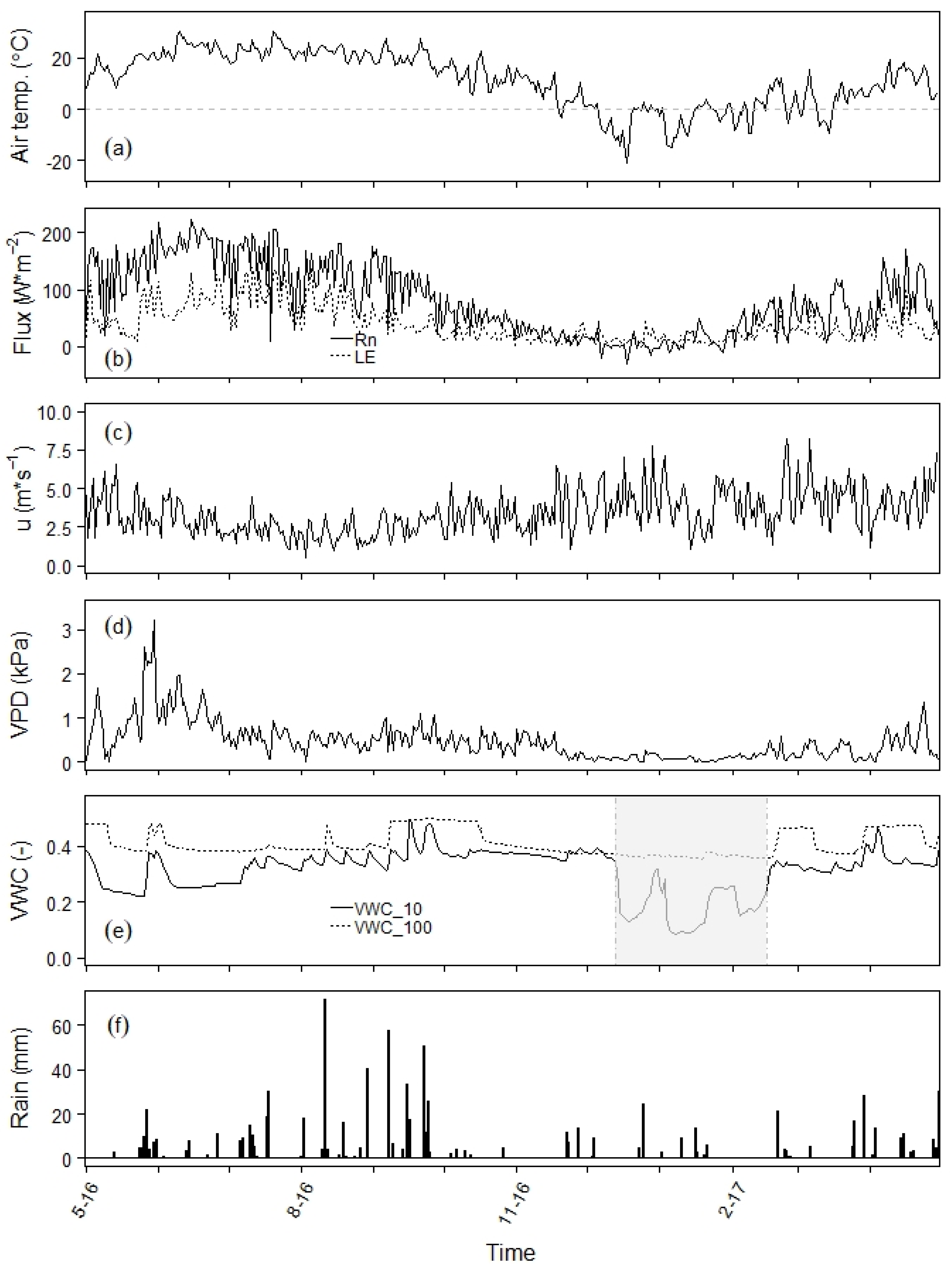
3.1. Regional Climate Conditions and Soil Moisture Dynamics

Figure 2 shows the annual changes of selected variables only from one of the EC towers (Tower 11), as the two tower sites showed similar trends in these variables over the year and Tower 11 had fewer missing data. The 15-min data were aggregated to a daily time scale for display in Figure 2.

The air temperature ranged between −20 and 30 °C over the year, reaching seasonal highs around June through August and lows between December and February. Net radiation data showed a very similar trend compared to air temperature seasonally. The Latent Heat Flux (LE) was higher during summer months, decreased in fall and winter, and then increased in spring (Figure 2a,b).

Wind speed at 2 m above ground (u) varies approximately between 0.5 and 8 m s⁻¹, with a pronounced daily shift between November 2016 and January through late February 2017. Relative Humidity (RH) fluctuated between 40 and 99%, except for a few days in late May 2016 (data not shown). Between July and September 2016, month-to-month scatterplot results showed that u and RH values had less day-to-day variation with smaller standard deviation compared to the rest of the months (data not shown), which also is seen in Figure 2c.

The Vapor Pressure Deficit (VPD) was calculated using mean temperature-based vapor pressure estimates described in Section 2. Mostly between zero and two of VPD were observed during the crop-growing season (May through October) except for a few days in late May. In late May, RH was extremely low (zero–0.19) and $e_s$ was higher than other times during the crop-growing season, thus this condition resulted in higher VPD in the range of 2.2 and 3.2 (Figure 2d).

Volumetric Water (soil moisture) Content (VWC) data were recorded from five depths (10, 20, 40, 60, and 100 cm), but we only present results at 10 cm (VWC_10) and 100 cm (VWC_100) below the ground to show the VWC near the surface and VWC from the deepest soil layer, respectively. We noticed that rainfall water constantly replenishes the surface soil layer after diminishing VWC. During the cold months of January and February 2017, VWC decreased close to 0.1 and gradually increased as spring approached, possibly due to the snowmelt and rainfall percolation. The surface soil was frozen between approximately 13 December, 2016 and 16 February, 2017. As expected, VWC from the deepest soil layer was relatively constant compared to the surface soil layer without big increases or declines during the study period. The VWC_100 data revealed that VWC reached the field capacity (near 0.49) after an intense rainfall during September. This occurred again in late February and early April 2017 (Figure 2e).

At Tower 11, the total annual rainfall amount measured during the study period was 863 mm. September was the wettest month of the study period (approximately 211 mm/month), accounting for approximately a quarter of the total amount of the annual rainfall. More than half of the annual rainfall fell between July and September 2016 (Figure 2f), resulting in a wet season in Iowa.

3.2. Energy Balance Closure

As a performance check of EC tower data, the energy balance closure was examined using four flux data of net radiation ($R_n$), soil heat flux ($G$), sensible heat flux ($H$), and latent heat flux ($LE$) [69]. The available energy ($R_n-G$) term needs to be balanced with the sum of $H$ and $LE$ [70]. The energy balance closure is estimated using the Energy Balance Ratio (EBR) defined in Equation (16) [71].

$$EBR=\frac{{{\displaystyle \sum }}_{t=1}^n\left(H+LE\right)}{{{\displaystyle \sum }}_{t=1}^n\left(R_n-G\right)}$$

(16)

where $t$ is time and $n$ is the last time step of energy fluxes. EBR was estimated for Towers 10 and 11 using 30-min aggregated four energy fluxes mentioned above during the study period. In addition, the available energy vs. $H$ + $LE$ was plotted for each site. Data also were divided into crop-growing season and no-crop season to investigate the effect of crop growth on EBR [8].

Table 1. Energy balance ratio (EBR) and slopes and intercepts from the relationship between $H$ + $LE$ and $R_n$ − $G$.

Methods		Tower #	Full Year (May 2016–April 2017)	Crop-Growing Season (May 2016–October 2016)	No-Crop Season (November 2016–April 2017)
EBR		10	0.77	0.72	0.93
		11	0.74	0.71	0.84
$H$ + $LE$ = m ($R_n$ − $G$) + b	m (slope)	10	0.59	0.61	0.53
		11	0.55	0.58	0.46
	b (intercept)	10	15.3	13.4	16.8
		11	15.6	15.2	15.9
	R2	10	0.9	0.94	0.79
		11	0.89	0.93	0.78

indicates that EBR from both towers was less than 0.8 for the entire study period and a little less than 0.75 during crop-growing season. However, the EBR values were higher during no-crop season than crop-growing season. In contrast, the relationship between available energy vs. sum of $H$ and $LE$ reveals that there was a high R² observed (R² > 0.9) during crop-growing season and the reverse during no-crop season.

3.3. Input Data Comparisons

The 15-min interval field input data were aggregated to hourly data (presented at all five x-axes in Figure 3) for comparison with input variables from the HRRR model (air temperature and RH in Figure 3a,e) or those from calculation results using HRRR data (Rn and u in Figure 3b–d).

In Figure 3e, only RH data of NWP outputs (y-axis) consist of RAP RH data (data obtained before 23 August) and HRRR RH data (on 23 August and after) as the version of the HRRR model before 23 August, 2016 did not generate RH; therefore RH values were taken from the RAP dataset of the same hour between 1 May and 22 August, 2016.

Tower 10 exhibited a very similar pattern of scatter plots (not shown). The R² values from Tower 10 were 0.99 (air temperature), 0.74 (HRRR Rn), 0.86 (HRRR-GOES Rn), 0.72 (u), and 0.81 (RH), revealing a little better agreement between observed Rn vs. HRRR Rn and worse agreement for HRRR-GOES Rn, u, and RH plots than those from Tower 11 (Figure 3). The air temperature showed a good agreement between field observation and HRRR input.

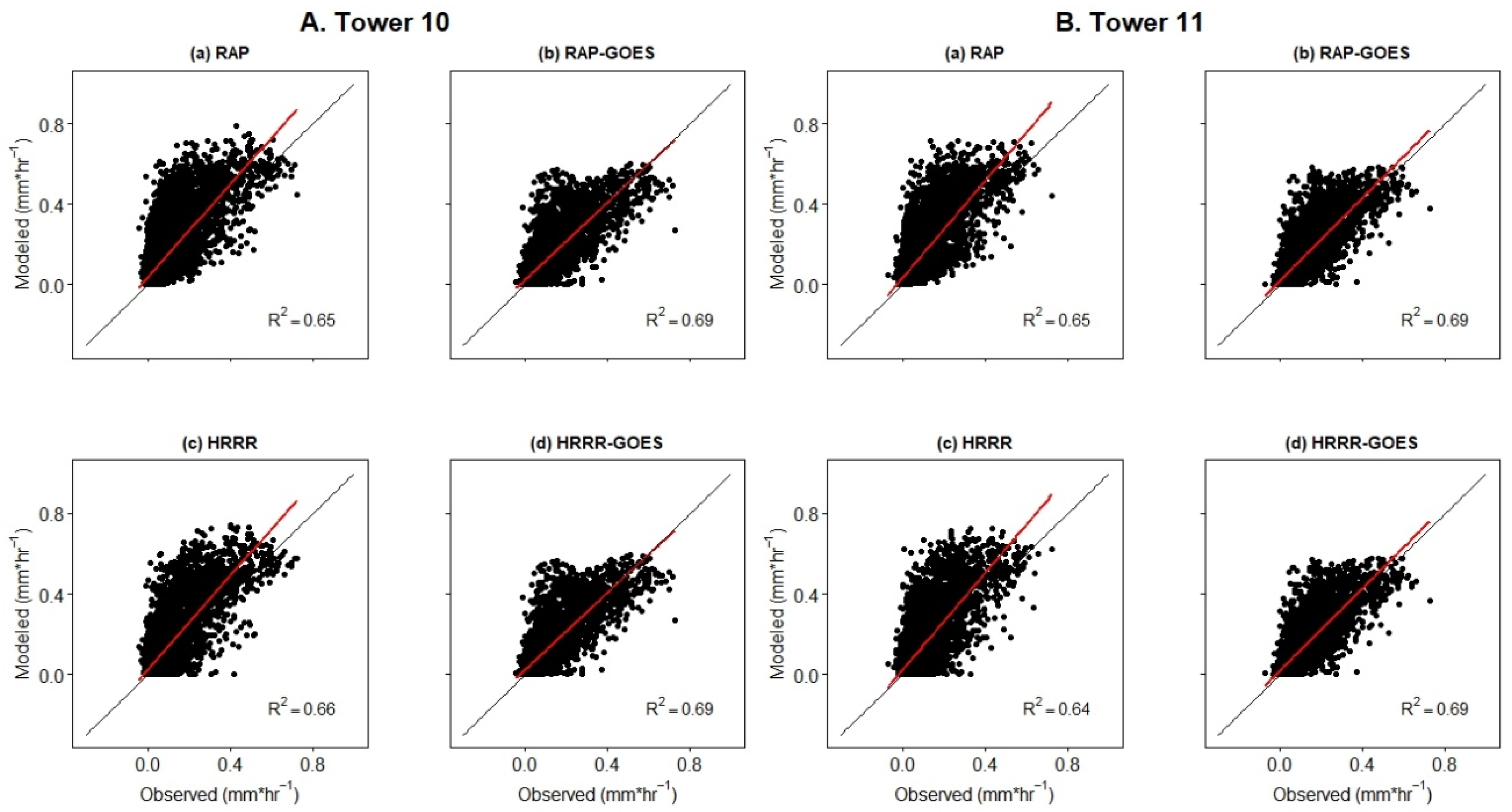
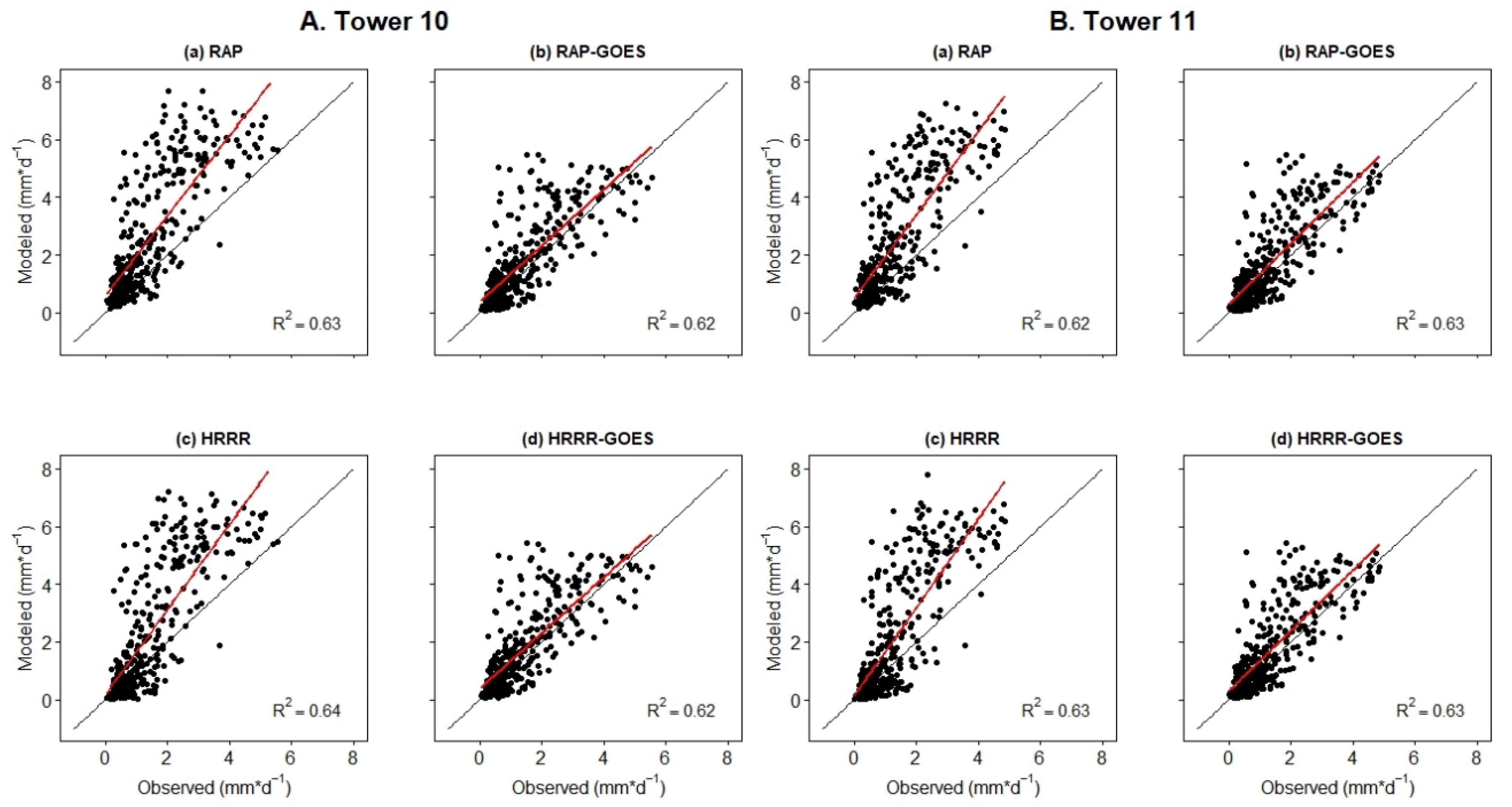
3.4. Observed vs. Modeled ET

In this paper, all AET data are presented in the unit of water depth (mm) per time. ET estimates from the NWP-based models and NWP-GOES-Rn models (called modeled AET hereafter) were validated against two EC tower measurements near central Iowa (called observed AET hereafter) for the duration of study period between May 2016 and April 2017. In Figure 4, hourly data between observed and modeled AET were compared by the model. As GOES-Rn data are included in both RAP and HRRR models, there was an increase in R² (compare (a) and (b) or (c) and (d) for each tower). In Figure 5, these hourly data were aggregated to the daily time scale and compared to the daily aggregated field ET data. There was little or no increase in R² as GOES-Rn data were used (Figure 5). One common observation from Figure 4 and Figure 5 is that a regression line gets closer to 1:1 line when GOES-Rn data were included.

Table 2. Root mean square error (RMSE) and mean bias (MB) results of modeled AET compared to the tower EC-derived AET for hourly and daily data during the study period.

Time Intervals	Data	Units	Tower #	RAP	RAP-GOES	HRRR	HRRR-GOES
Hourly	RMSE	mm hr−1	10	0.1	0.08	0.09	0.08
			11	0.1	0.08	0.09	0.07
	MB	mm hr−1	10	0.05	0.02	0.04	0.02
			11	0.05	0.02	0.04	0.02
Daily	RMSE	mm d−1	10	1.79	0.99	1.69	0.98
			11	1.78	0.99	1.7	0.98
	MB	mm d−1	10	1.15	0.34	0.86	0.34
			11	1.13	0.38	0.87	0.37

shows the RMSE and MB results to further investigate the relationships between observed and modeled AET data. For both RMSE and MB, data were improved by the inclusion of GOES-R into the models. In general, HRRR and HRRR-GOES produced better results than RAP and RAP-GOES, respectively, in terms of RMSE and MB. As shown with the change in RMSE, the Mean Absolute Error (MAE) has the same trend resulting in the highest MAE with RAP, then a little less with HRRR than RAP, and less with RAP-GOES and HRRR-GOES (data not shown). The Spearman correlation coefficient ($\rho$) results of hourly AET data for the entire year showed that infusing GOES-Rn into RAP and HRRR improved $\rho$ by 12 and 17% for Tower 10, respectively, and 10 and 15% for Tower 11, respectively (

Table 3. Spearman correlation coefficients ($\rho$) of the modeled AET against observed AET using hourly and daily data with respect to yearly and seasonal (four-month intervals) duration.

Time Intervals	Duration of Data	Tower #	RAP	RAP-GOES	HRRR	HRRR-GOES
Hourly	Full year	10	0.68	0.8	0.63	0.8
		11	0.7	0.8	0.65	0.8
	MJJA	10	0.83	0.84	0.85	0.84
		11	0.84	0.86	0.85	0.86
	SOND	10	0.71	0.75	0.67	0.76
		11	0.7	0.74	0.68	0.74
	JFMA	10	0.62	0.68	0.65	0.68
		11	0.62	0.7	0.63	0.68
Daily	Full year	10	0.8	0.8	0.8	0.8
		11	0.79	0.8	0.8	0.8
	MJJA	10	0.49	0.43	0.51	0.43
		11	0.51	0.51	0.51	0.51
	SOND	10	0.63	0.61	0.64	0.61
		11	0.61	0.62	0.63	0.62
	JFMA	10	0.66	0.73	0.67	0.73
		11	0.65	0.73	0.68	0.73

). The warm season (May through August) $\rho$ results for both towers were highest compared to other seasons, indicating that there is a strong correlation between tower AET and modeled AET with hourly data. However, when the data were aggregated to the daily time scale, the $\rho$ from the warm season showed the lowest correlation compared to other seasons. With the daily time scale data, the full year data of $\rho$ shows the best result compared to other seasonal $\rho$ data from the daily time scale.

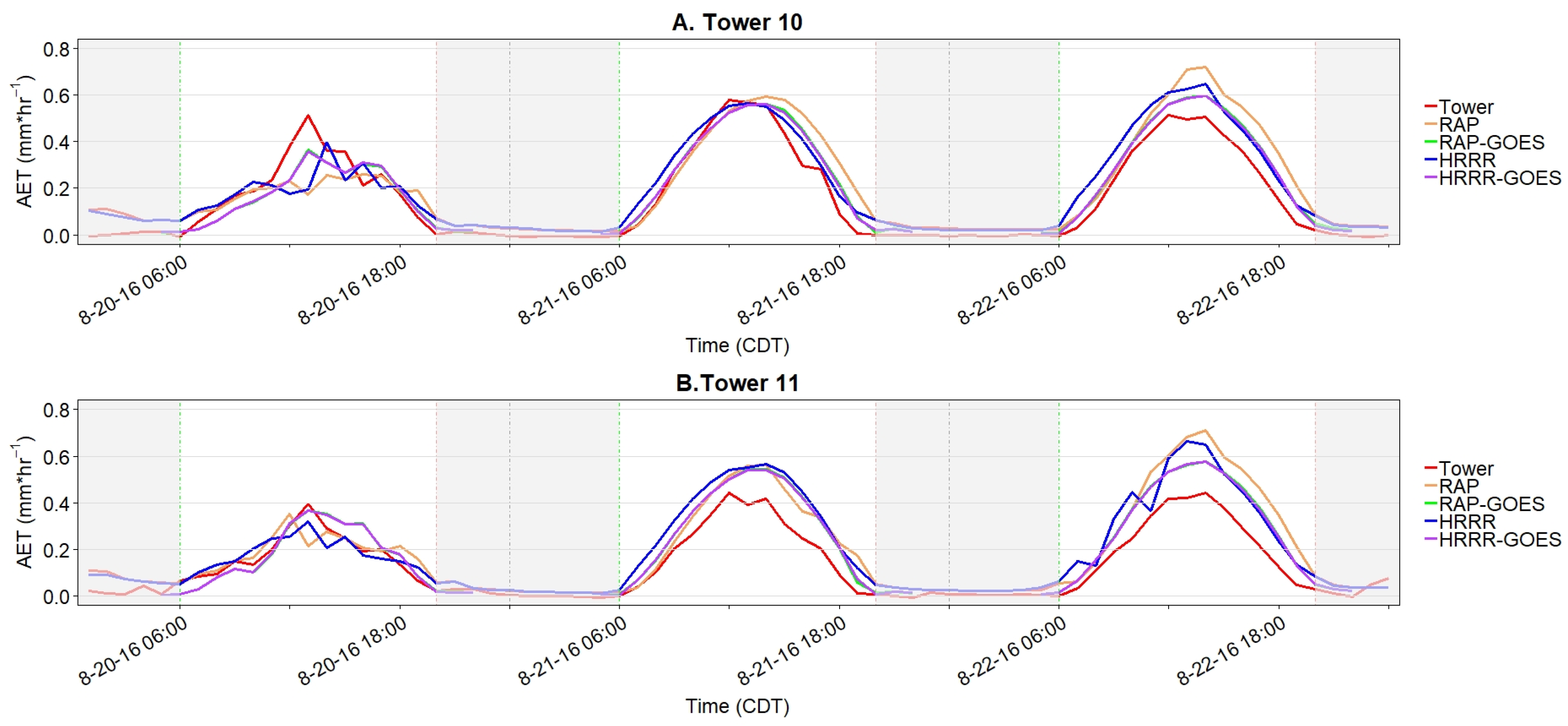
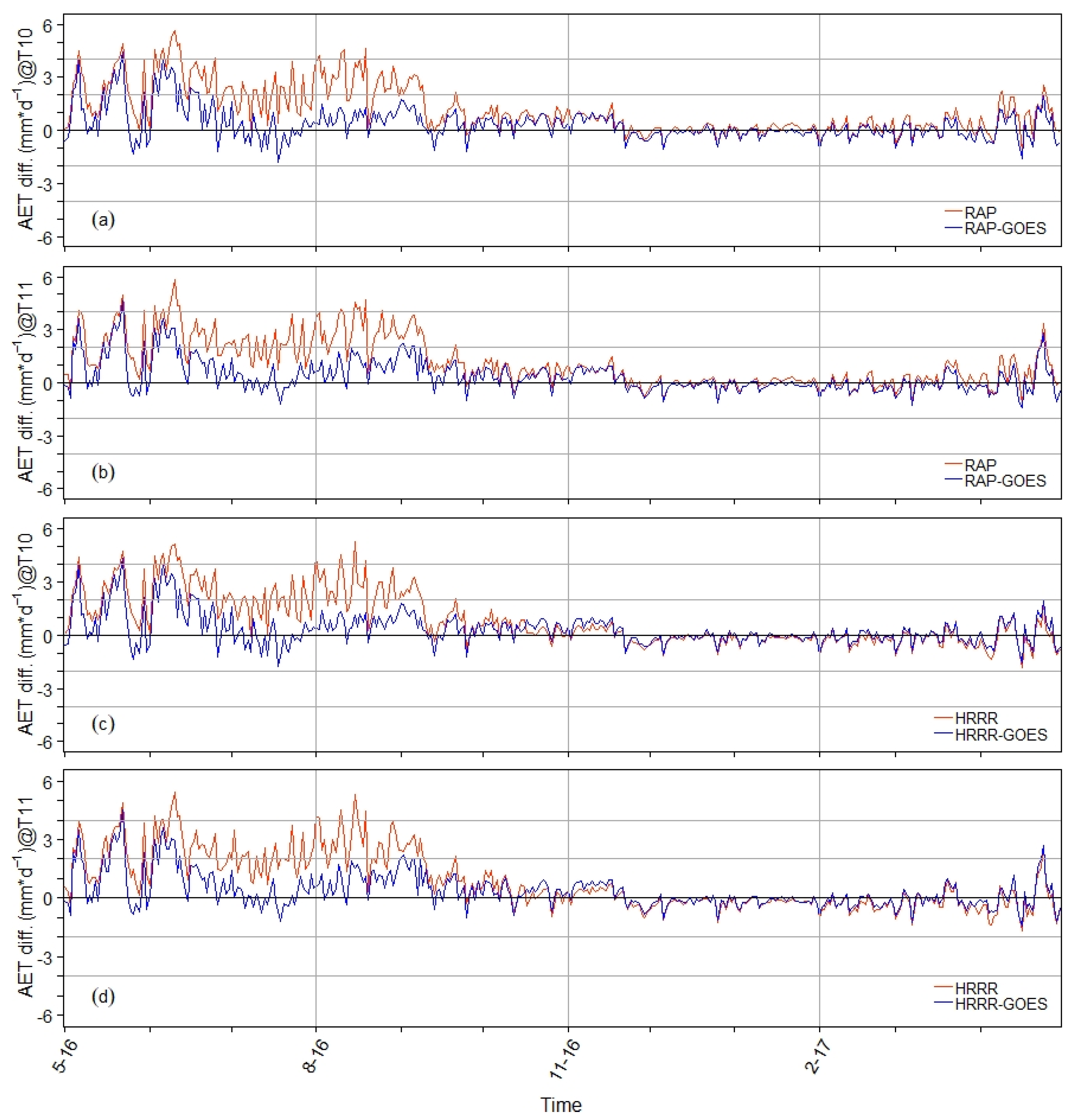
3.5. Temporal ET Changes

Figure 6 shows hourly AET changes of the four models during three random consecutive days in August to demonstrate how models match field observation. Gray areas represent approximately no sunshine hours for the selected days. There was no rain for the three days, except for a few hours of light rain on 20 August. For the three-day period, averaged daily Rn (W m⁻²) was 97.6, 163.7, 165.2, respectively, for Tower 10, and 97.2, 143.6, 151.0, respectively, for Tower 11. During no-sunshine hours (mostly late at night and early in the morning), models tend to overpredict AET compared to the tower AET data. Modeled AET data from 20 August appear to match quite well with tower AET data for a few hours, then tower AET shows the highest peak between 12:00 and 1:00 PM at Tower 10. RAP-GOES and HRR-GOES AET data tend to predict AET pretty closely to tower AET data in the morning of 21 August. On 22 August, all modeled AET tend to overpredict tower AET. The RAP and HRRR model predictions on 22 August were relatively higher than other GOES-based models and field observation (Figure 6).

Figure 7 shows the difference between the modeled AET and observed AET in the daily time scale. Between approximately May and mid-September 2016, modeled RAP and HRRR model results especially showed a big difference between modeled and observed AETs. Less difference is shown until November 2016 with RAP, and until around October 2016 with HRRR. Adding GOES-Rn did not improve the difference very much between May and July 2016, however inclusion of GOES-Rn greatly improved model AET estimates especially after July 2016.

The HRRR results showed some improvement (Figure 7c,d) over their RAP counterparts from Figure 7a,b by showing less AET difference. There was no distinguishable difference between sites ((a) vs. (b) or (c) vs. (d)).

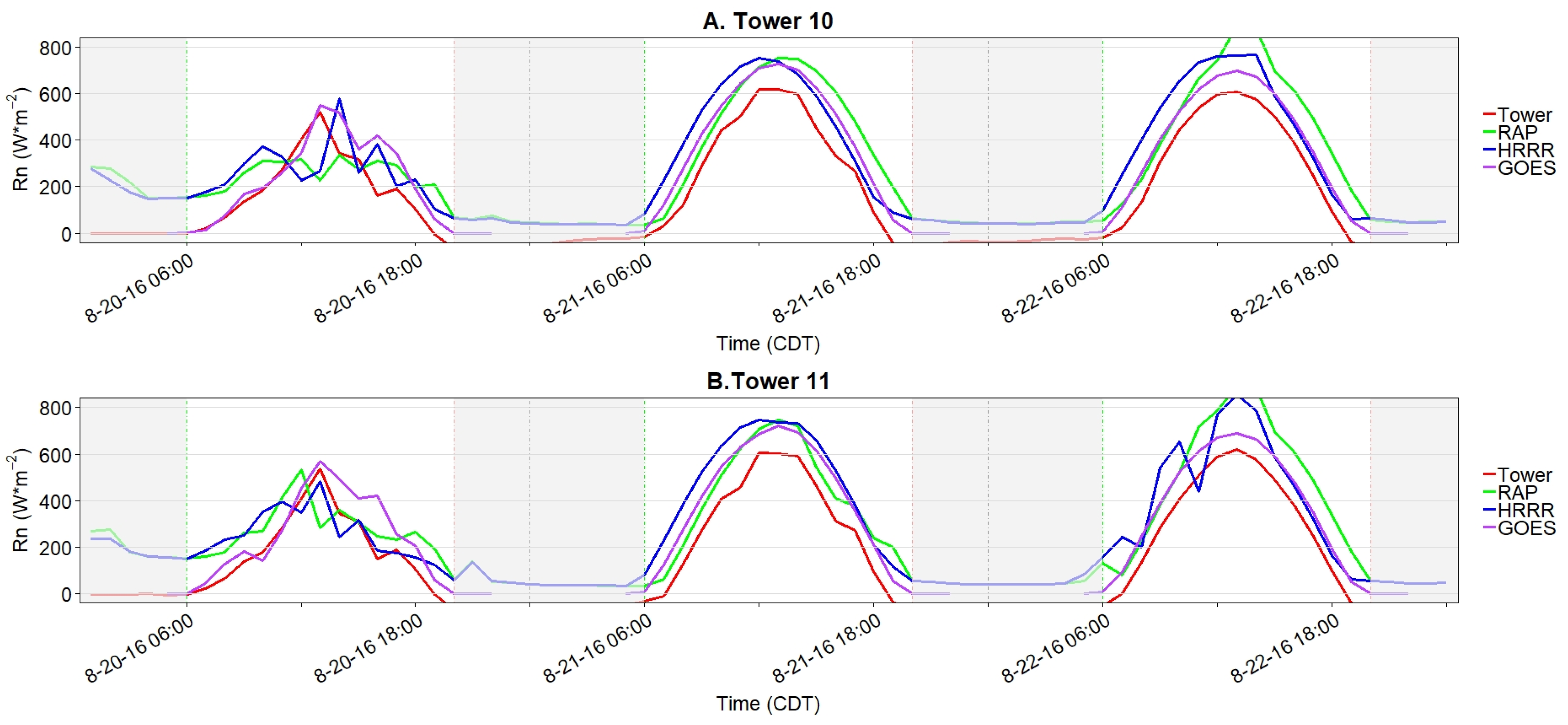
3.6. Temporal Rn Changes

In Figure 8, the Rn results from three days that match the selected days in Figure 6 showed a diurnal fluctuation throughout day and night as the AET changes in Figure 6. The RAP and HRRR results appear to overestimate Rn, the most compared to tower Rn. GOES-Rn results were close to tower Rn in the morning of 20 August, however overprediction of GOES-Rn was observed during the afternoon. The GOES-Rn data were a little higher than tower Rn for the next two days. Overall, GOES-Rn data were closer to tower Rn than the RAP- and HRRR-produced Rn. RAP and HRRR Rn also overpredicted tower Rn around sunset hours. As GOES-Rn were available for only 18 h a day, there was no comparison between GOES-Rn and tower Rn between 11:00 PM and 4:00 AM each day.

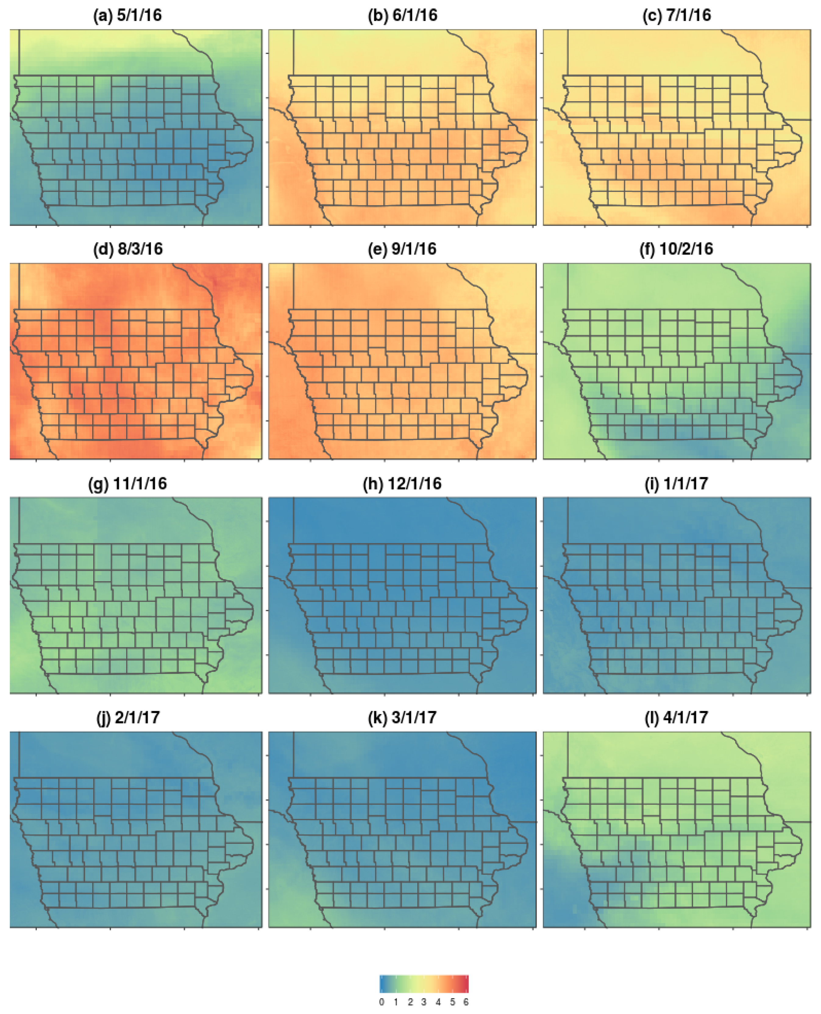
3.7. Spatial ET Distributions

Figure 9 depicts the daily total AET distribution over the state of Iowa using HRRR-GOES data. We chose the HRRR-GOES dataset for AET maps in Figure 9 from the four available datasets because HRRR-GOES showed the best performance result by introducing the least RMSE and MB, and higher $\rho$ (Table 2 and Table 3). Only one day per month (generally the first day of the month) was selected here to represent the daily AET trend in time and space during the study period. For the months of August and October 2016, the next available non-rainy day was selected, as the first days of these two months were rainy days based on EC tower rainfall data.

It is clear that the summer to early fall months (June through September) have higher daily AET than other months due to higher Rn and air temperature observed during these months (Figure 2). Moreover, there was more available water from the rainfall, which contributes to higher AET during these months. AET becomes less as the cold months (December through February) approach. Following the cold months, AET increases gradually as more incoming Rn is available in March and April. There was no specific trend of higher or lower AET observed between the areas. Southern Minnesota and northern Iowa got a little bit higher estimated AET than other areas in May and October 2016. During the summer months for those selected days, the AET distribution varies. These AET maps seem to show that there are AET values during winter months, although they are much smaller than summer month estimates.

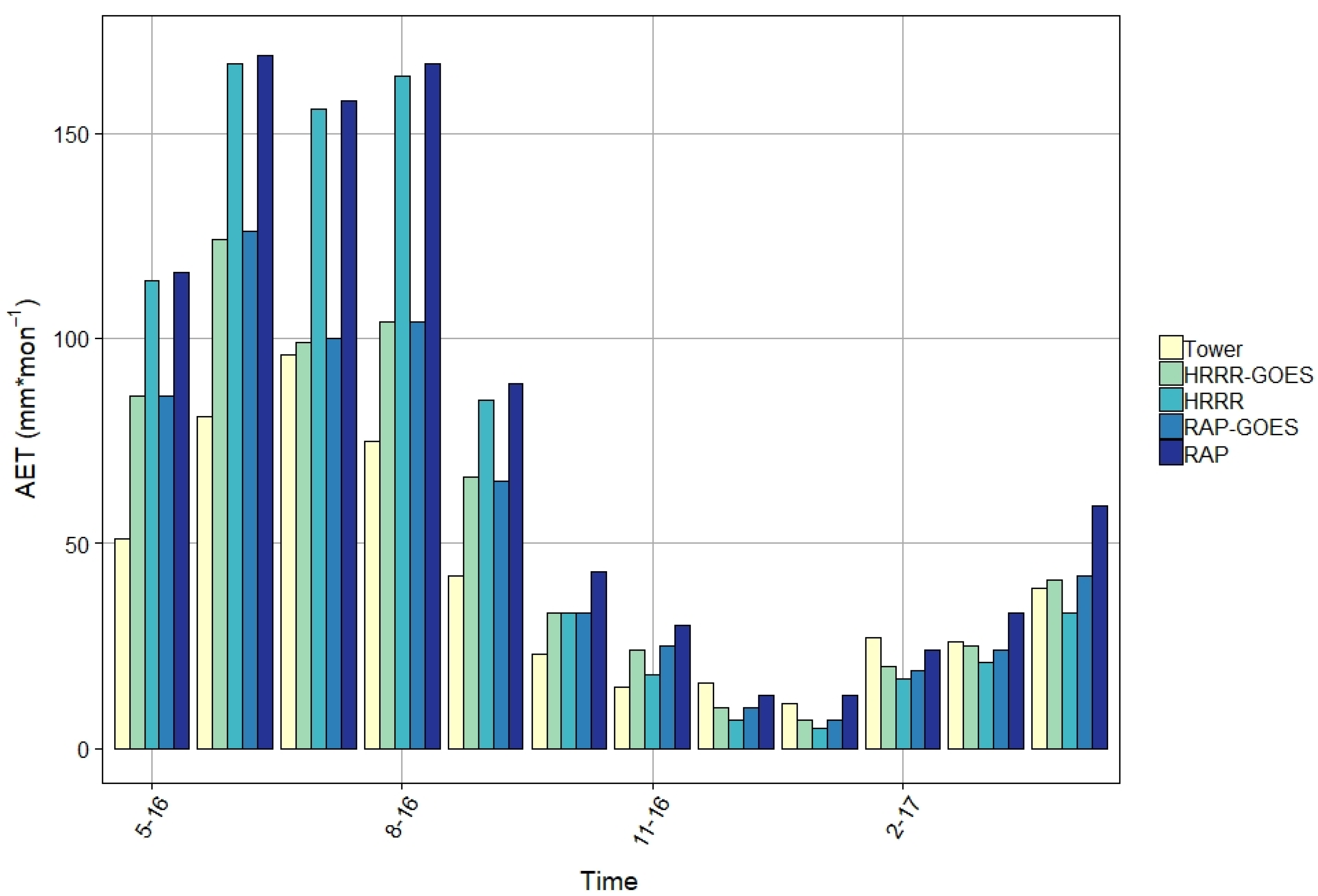
3.8. Monthly Total ET Comparisons

Hourly AET estimates from the four models and 15-min field AET observations were aggregated to the monthly time scale for a seasonal comparison of the total AET estimates. Figure 9 indicates that monthly observed AET data tend to be smaller than all other modeled AET data especially during crop-growing season (May through October 2016). The RAP-GOES and HRRR-GOES models appear to improve monthly AET estimates compared to RAP and HRRR, respectively. For the cold months between December 2016 and March 2017, modeled AET data were less than the monthly total observed AET. During this time, HRRR appears to show the smallest AET estimates in the monthly time scale, which is quite the opposite of warmer months (May through September 2016), when HRRR ranked the second highest in monthly total AET estimates. AET estimates from RAP were the highest most of the time, except for December 2016 and February 2017.

4. Discussion

Estimated EBR from the two towers in this study (0.77 and 0.74 for the entire year) tend to agree with the published results [4,72]. Twine et al. [4] reported the EBR values of nine grassland field sites in Oklahoma for two months (June and July) in 1997 ranging between 0.72 and 0.91 using 30-min averaged energy fluxes. Wilson et al. [72] showed the annual EBR values for various landscapes between 0.34 and 1.69. EBR data from the maize site in Bonville, Illinois varied between 0.7 and 1.2 by year, which could be comparable to the EC data we used in this study. Hernandez-Ramirez et al. [8] stated that the four-year (2004–2007) mean annual EBR values using 15-min averaged data for corn and soybean crops in central Iowa were 0.87 and 0.81, respectively, which were higher than our results. Their EBR data for corn and soybean during the crop-growing season and no-crop seasons were 0.87 and 0.82, respectively, for the crop-growing season and 0.90 and 0.78, respectively, for no-crop season. There was no difference in EBR between the crop-growing season and no-crop season when the mean values (0.84) of these two seasons were compared. This is somewhat different from our study. The EBR from our study revealed values during the crop-growing season smaller than those from the no-crop season (0.72 vs. 0.93 for Tower 10 and 0.71 vs. 0.84 for Tower 11, respectively).

During the crop-growing season in Iowa, a high magnitude of LE was observed (the six-month cumulative total is approximately 1685 MJ m⁻² using 30-min data; data not shown). Whereas, the H value showed a smaller quantity (869 MJ m⁻²) than LE. The wind speed during this season was lower than that of the no-crop season (2.8 vs. 4.0 m s⁻¹). Moreover, the dew point temperature and relative humidity (RH) were high. All these conditions cause the atmospheric boundary layer to thin, which results in small eddy diffusivity. These combined field conditions contributed to a low energy balance ratio for the crop-growing field (personal communication with Dr. John M. Norman).

The slope of ($R_n-G$) vs. ($H+LE$) was less than one and the intercept was larger than zero for all seasons. This was typically noticed when the energy balance was not closed with the EC system [4,72]. This also was acknowledged by Scott [21]. Scott [21] pointed out that this meant that the H + LE term is greater than Rn-G for lower Rn-G values and less than Rn-G for higher Rn-G, which exactly depicts the results of EC tower data in this study.

The vapor pressure deficit (VPD) increased between May and mid-June 2016 as the RH was relatively lower (approximately 55% on average; data not shown) than during the fall season (approximately 75% on average between September and November) and the high Rn (approximately 143 W m⁻² on average) from Figure 2. About 52 W m⁻² of Rn was partitioned to LE (36%) at the same time. In particular, the high VPD in late May 2016 was caused by a very low RH observed at the same time (data not shown) and the increasing air temperature.

The ratio of monthly summed LE/monthly summed Rn using daily averaged LE and Rn flux data (Figure 2b) increased as summer approached, reaching peak values of LE/Rn in July and August 2016 during the crop-growing season (0.6 and 0.56, respectively; data not shown). Then, the LE/Rn decreased as winter approached. More than 50% of Rn was used for the LE flux, indicating that there was a high demand for water by plants through the transpiration process and in the air. During December and January, the daily Rn had numerous negative values, therefore the sum of Rn is smaller than that of LE in those months. Therefore, the comparison between monthly LE/monthly Rn during the crop-growing season and during winter is not valid in this case.

The VWC near the ground surface fluctuated between 0.22 and 0.49 during the crop-growing season. The VWC at the soil surface (VWC_10) increased due to the frequent rainfall in late May 2016, then decreased as water evaporated and was used by crops. The VWC trend was not easy to track when there was a small amount of rain (e.g., a few rainfall events in mid and late June 2016). However, in July through September numerous rainfall events occurred, accounting for more than 50% of the annual rainfall at the tower site. The VWC_10 changed along the time by showing that the fluctuation of VWC continued and the highest VWC in a year occurred, possibly due to accumulation of water at the surface without losing much water. This was anticipated because it occurred at the time when crop growth reached its maturity. The VWC from the surface soil layer fluctuated more than the deepest layer VWC, indicating that the water content changed due to the interactions between soil surface and atmospheric layer from solar radiation, wind, and ET (Figure 2d).

Air temperature data between HRRR inputs and field observations especially show a very high R² value of 0.99 (Figure 3a). This might indicate that the HRRR-based air temperature could be used for PM-ET when the field air temperature data are not available. In the PM method, $e_s$, $e$, $\Delta$, and ${\rho }_a$ are directly estimated using a 2 m air temperature. Therefore, the accurately estimated 2 m air temperature is of good use for PM-based ET estimates.

The $R_n$ estimation from RAP and HRRR models based in Equation (1) was higher than the field and GOES-$R_n$ (Figure 8). This might mean that there could be higher downward short- or long-wave radiation flux or smaller upward short- or long-wave radiation flux from the NWP-based models.

As the time scale was aggregated from hour to day, the difference in AET became larger (Figure 7). When the hourly data were aggregated, the discrepancy between observed and modeled LE became larger during summer months than winter months, as there was a big difference observed at night between modeled and observed AET data. Thus, this overpredicted nighttime modeled AET contributed to a much higher modeled AET than observed AET.

The monthly total AET results were compared to the historical NLDAS data that were monthly averaged between 2002 and 2010 (data not shown; NLDAS data were prepared by Dr. Walter Navarro). The spatial coverage of NLDAS data was the entire state of Iowa. The NLDAS monthly AET was close to the EC tower AET data except for July and August. In those months, NLDAS AET was bigger than AET from the two towers (121 vs. 103 from Tower 10, and 121 vs. 96 from Tower 11 in July; 112 vs. 85 from Tower 10, and 112 vs. 75 from Tower 11 in August) (Figure 10). Although the NLDAS data represented the state of Iowa and tower EC data came from two fields near central Iowa, these two datasets were in agreement with each other.

5. Conclusions and Future Directions

This study explores the possibility of using NWP models to estimate hourly ET in near real-time. A numerical study using one-year data showed that the proposed NWP-based ET model was capable of estimating operational hourly ET in near real-time. Hourly, daily, and monthly modeled AET data were compared against two EC tower measurements to validate how model results would match field observations. Hourly data matched well with the field EC data, however, when data were aggregated to daily and monthly time scales, results did not tend to match with the field EC data. Overall, suggested NWP-based ET models with the inclusion of GOES-$R_n$ worked better than NWP-only ET models with statistical results of lower RMSE, MAE, and ME, and higher $\rho$ and R². The HRRR-GOES ET model showed the best model results when compared to the field observation. Although model validations with more EC field site data are required, the suggested HRRR-GOES model appears to be usable for near real-time operational ET estimates by showing an improved performance compared to the HRRR model.

In this study, we implemented the expected Kc values based on the FAO-56 report with an assumption that the ET model has a constant Kc for the entire model domain with fixed percentages of corn and soybean crops (60 and 40%, respectively). This is a very simplified and idealized approach to test our proposed NWP-based ET estimates. The approach has to be improved to obtain more realistic ET estimates over the regional scale. To accomplish this goal, we are working on updating this simple Kc with the MODIS-based Kc method to rescale PET to AET. This new implementation will provide better Kc data by depicting the spatial distribution of Kc.

Although we ruled out the use of other NWP, numerical models, and RS products for input data due to the unavailability of obtaining minimum latency (<a few hours) and larger spatial domain (>10 km) of other NWP products or a long re-visit time from a high spatial resolution RS product just to meet with our needs to produce a near real-time operational ET estimation tool, we plan to test our models with a few selected products for further validations (for example, NLDAS-2, NOAA models, and WRF-Hydro, or LANDSAT, MODIS, and AVHRR products).

The NWP outputs currently generate data with up to 21 (for RAP) and 18 (for HRRR) h of lead time. This certainly allows us to utilize NWP products for ET forecasting. The authors’ future plan could expand the use of NWP for real-time operational ET forecasting on top of the now-casting production, which helps promote the use of ET for the operational hydrologic model.

This study has been limited to the Iowa domain using data from only two EC towers for model validation. It would be interesting to investigate how well this NWP-based ET model works in other regions by testing it with EC data from other climate zones in the United States. More robust model tests with more widely distributed EC tower data would be required to further prove the usability of the NWP-based ET model for near real-time ET estimation.

References

1. Brutsaert, W. Evaporation into the Atmosphere: Theory, History, and Applications; Kluwer Academic Publisher: Dordrecht, The Netherlands; Boston, MA, USA; London, UK, 1982. [Google Scholar]
2. Margulis, S.A.; Entekhabi, D. Feedback between the land surface energy balance and atmospheric boundary layer diagnosed through a model and its adjoint. J. Hydrometeorol. 2001, 2, 599–620. [Google Scholar] [CrossRef]
3. Katul, G.G.; Oren, R.; Manzoni, S.; Higgins, C.; Parlange, M.B. Evapotranspiration: A process driving mass transport and energy exchange in the soil-plant-atmosphere-climate system. Rev. Geophys. 2012, 50, RG3002. [Google Scholar] [CrossRef] [Green Version]
4. Twine, T.E.; Kustas, W.P.; Norman, J.M.; Cook, D.R.; Houser, P.R.; Meyers, T.P.; Prueger, J.H.; Starks, P.J.; Wesely, M.L. Correcting eddy-covariance flux understimates over a grassland. Agric. For. Met. 2000, 103, 279–300. [Google Scholar] [CrossRef] [Green Version]
5. Batra, N.; Islam, S.; Venturini, V.; Bisht, G.; Jiang, L. Estimation and comparison of evapotranspiration from MODIS and AVHRR sensors for clear sky days over the Southern Great Plains. Remote Sens. Environ. 2006, 103, 1–15. [Google Scholar] [CrossRef]
6. Oleson, K.W.; Niu, G.-Y.; Yang, Z.-L.; Lawrence, D.M.; Thornton, P.E.; Lawrence, P.J.; Stöckli, R.; Dickinson, R.E.; Bonan, G.B.; Levis, S.; et al. Improvements to the community land model and their impact on the hydrological cycle. J. Geophys. Res. 2008, 113, G01021. [Google Scholar] [CrossRef]
7. Parr, D.; Wang, G.; Fu, C. Understanding evapotranspiration trends and their driving mechanisms over the NLDAS domain based on numerical experiments using CLM4.5. J. Geophys. Res. Atmos. 2016, 121, 7729–7745. [Google Scholar] [CrossRef] [Green Version]
8. Hernandez-Ramirez, G.; Hatfield, J.L.; Prueger, J.H.; Sauer, T.J. Energy balance and turbulent flux partitioning in a corn-soybean rotation in the Midwestern US. Appl. Clim. 2010, 100, 79–92. [Google Scholar] [CrossRef]
9. Hernandez-Ramirez, G.; Hatfield, J.L.; Parkin, T.B.; Sauer, T.J.; Prueger, J.H. Carbon dioxide fluxes in corn-soybean rotation in the miswestern U.S.: Inter- and intra-annual variations, and biophysical controls. Agric. For. Met. 2011, 151, 1831–1842. [Google Scholar] [CrossRef] [Green Version]
10. Baldocchi, D.D.; Vogel, C.A. Seasonal variation of energy and water vapor exchange rates above and below a boreal jack pine forest canopy. J. Geophys. Res. 1997, 102, 28939–28951. [Google Scholar] [CrossRef]
11. Jung, M.; Reichstein, M.; Ciais, P.; Seneviratne, S.I.; Sheffield, J.; Goulden, M.L.; Bonan, G.; Cescatti, A.; Chen, J.; De Jeu, R.; et al. Recent decline in the global land evapotranspiration trend due to limited moisture supply. Nature 2010, 467, 951–954. [Google Scholar] [CrossRef]
12. Qin, L.; Xi, C.; Ying, L.; BaoAn, M.; Frank, V. Regional evapotranspiration retrieval in arid areas. J. Arid Land Resour. Environ. 2012, 26, 1–9. [Google Scholar]
13. Trenberth, K.E.; Smith, L.; Qian, T.; Dai, A.; Fasullo, J. Estimates of the global water budget and its annual cycle using observational and model data. J. Hydrometeorol. 2007, 8, 758–769. [Google Scholar] [CrossRef]
14. Koster, R.D.; Dirmeyer, P.A.; Guo, Z.; Bonan, G.; Chan, D.; Cox, P.; Gordon, C.T.; Kanae, S.; Kowalczyk, E.; Lawrence, D.; et al. Regions of strong coupling between soil moisture and precipitation. Science 2004, 305, 1138–1140. [Google Scholar] [CrossRef] [PubMed] [Green Version]
15. McVicar, T.R.; Jupp, D.L.B. The current and potential operational uses of remote sensing to aid decisions on drought exceptional circumstances in Australia: A review. Agric. Syst. 1998, 57, 399–468. [Google Scholar] [CrossRef]
16. Anderson, M.C.; Norman, J.M.; Mecikalski, J.R.; Otkin, J.A.; Kustas, W.P. A climatological study of evapotranspiration and moisture stress across the continental United States based on thermal remote sensing: 1. Model formulation. J. Geophys. Res. 2007, 112, D10117. [Google Scholar] [CrossRef]
17. Mo, S.; Liu, S.; Lin, Z.; Wang, S.; Hu, S. Trends in land surface evapotranspiration across China with remotely sensed NDVI and climatological data for 1981–2010. Hydrol. Sci. J. 2015, 60, 2163–2177. [Google Scholar] [CrossRef] [Green Version]
18. Tian, D.; Martinez, C.J. Forecasting reference evapotranspiration using retrospective forecast analogs in the southeastern United States. J. Hydrometeorol. 2012, 13, 1874–1892. [Google Scholar] [CrossRef]
19. Howell, T.A.; Schneider, A.D.; Jensen, M.E. History of lysimeter design and use for evapotranspiration measurements. In Proceedings of the ASCE International Symposium on Lysimetry: Lysimeters for Evapotranspiration and Environmental Measurements; Allen, R.G., Howell, T.A., Pruitt, W.O., Walter, I.A., Jensen, M.E., Eds.; ASCE: New York, NY, USA, 1991; pp. 1–9. [Google Scholar]
20. Bowen, I.S. The ratio of heat losses by conduction and by evaporation from any water surface. Phys. Rev. 1926, 27, 779–787. [Google Scholar] [CrossRef] [Green Version]
21. Scott, R.L. Using watershed water balance to evaluate the accuracy of eddy covariance evaporation measurements for three semiarid ecosystems. Agric. For. Met. 2010, 150, 219–225. [Google Scholar] [CrossRef]
22. Farahani, H.J.; Howell, T.A.; Shuttleworth, W.J.; Bausch, W.C. Evapotranspiration: Progress in measurement and modeling in agriculture. Trans. Asabe 2007, 50, 1627–1638. [Google Scholar] [CrossRef]
23. Shuttleworth, W.J. Evapotranspiration measurement methods. Southwest Hydrol. 2008, 7, 22–23. [Google Scholar]
24. Eugster, W.; Merbold, L. Eddy covariance for quantifying trace gas fluxes from soils. Soil 2015, 1, 187–205. [Google Scholar] [CrossRef] [Green Version]
25. Gowda, P.H.; Chavez, J.L.; Colaizzi, P.D.; Evett, S.R.; Howell, T.A.; Tolk, J.A. ET mapping for agricultural water management: Present status and challenges. Irrig. Sci. 2008, 26, 223–237. [Google Scholar] [CrossRef] [Green Version]
26. Zhang, K.; Kimball, J.S.; Running, S.W. A review of remote sensing based actual evapotranspiration estimation. Wires Water 2016, 3, 834–853. [Google Scholar] [CrossRef]
27. Cihlar, J.; Ly, H.; Li, Z.; Chen, J.; Pokrant, H.; Huang, F. Multitemporal, multichannel AVHRR data sets for land biosphere studies – Artifacts and corrections. Remote Sens. Environ. 1997, 60, 35–57. [Google Scholar] [CrossRef]
28. Chien, S.; Mclaren, D.; Doubleday, J.; Tran, D.; Tanpipat, V. Using taskable remote sensing in a sensor web for Thailand flood monitoring. J. Aerosp. Inf. Syst. 2019, 16, 107–119. [Google Scholar] [CrossRef]
29. Bastiaanssen, W.G.M.; Menenti, M.; Feddes, R.A.; Holtslag, A.A.M. A remote sensing surface energy balance algorithm for land (SEBAL). J. Hydrol. 1998, 212–213, 198–212. [Google Scholar] [CrossRef]
30. Allen, R.G.; Tasumi, M.; Trezza, R. Satellite-based energy balance for mapping evapotranspiration with internalized calibration (METRIC)–Model. Asce J. Irrig. Drain. Eng. 2007, 133, 380–394. [Google Scholar] [CrossRef]
31. Jiang, C.; Guan, K.; Pan, M.; Ryu, Y.; Peng, B.; Wang, S. BESS-STAIR: A framework to estimate daily, 30 m, and all-weather crop evapotranspiration using multi-source satellite data for the US Corn Belt. Hydrol. Earth Syst. Sci. 2020, 24, 1251–1273. [Google Scholar] [CrossRef] [Green Version]
32. Wan, Z.; Wang, P.; Li, X. Using MODIS land surface temperature and normalized difference vegetation index products for monitoring drought in the southern Great Plains, USA. Int. J. Remote Sens. 2004, 25, 261–274. [Google Scholar] [CrossRef]
33. Vinukollu, R.K.; Wood, E.F.; Ferguson, C.R.; Fisher, J.B. Global estimates of evapotranspiration for climate studies using multi-sensor remote sensing data: Evaluation of three process-based approaches. Rem. Sens. Environ. 2011, 115, 801–823. [Google Scholar] [CrossRef]
34. Price, J.C. Estimating surface temperatures from satellite thermal infrared data—A simple formulation for the atmospheric effect. Rem. Sens. Environ. 1983, 13, 353–361. [Google Scholar] [CrossRef]
35. Diak, G.R.; Anderson, M.C.; Bland, W.L.; Norman, J.M.; Mecikalski, J.M.; Aune, R.M. Agricultural management decision aids driven by real-time satellite data. Bull. Am. Met. Soc. 1998, 79, 1345–1355. [Google Scholar] [CrossRef] [Green Version]
36. Jacobs, J.M.; Anderson, M.C.; Friess, L.C.; Diak, G.R. Solar radiation, longwave radiation and emergent wetland evapotranspiration estimates from satellite data in Florida, USA. Hydrol. Sci. J. 2004, 49, 461–476. [Google Scholar] [CrossRef]
37. Mitchell, K.E.; Lohmann, D.; Houser, P.R.; Wood, E.F.; Schaake, J.C.; Robock, A.; Cosgrove, B.A.; Sheffield, J.; Duan, Q.; Luo, L.; et al. The multi-institution North American Land Data Assimilation System (NLDAS): Utilizing multiple GCIP products and partners in a continental distributed hydrological modeling system. J. Geophys. Res. 2004, 109, D07S90. [Google Scholar] [CrossRef] [Green Version]
38. Xia, Y.; Mitchell, K.; Ek, M.; Sheffield, J.; Cosgrove, B.; Wood, E.; Luo, L.; Alonge, C.; Wei, H.; Meng, J.; et al. Continental-scale water and energy flux analysis and validation for the North American Land Data Assimilation System project phase 2 (NLDAS-2): 1. Intercomparison and application of model products. J. Geophys. Res. 2012, 117, D03109. [Google Scholar] [CrossRef]
39. Nearing, G.S.; Mocko, D.M.; Peters-Lidard, C.D.; Kumar, S.V.; Xia, Y. Benchmarking NLDAS-2 soil moisture and evapotranspiration to separate uncertainty contributions. J. Hydrometeorol. 2016, 17, 745–759. [Google Scholar] [CrossRef]
40. Gochis, D.J.; Yu, W.; Yates, D.N. The WRF-Hydro Model Technical Description and User’s Guide; Version 3.0, NCAR Technical Document; 2015; 120p, Available online: http://www.ral.ucar.edu/projects/wrf_hydro/ (accessed on 9 March 2017).
41. Kioutsioukis, I.; de Meij, A.; Jakobs, H.; Katragkou, E.; Vinuesa, J.-F.; Kazantzidis, A. High resolution WRF ensemble forecasting for irrigation: Multi-variable evaluation. Atmos. Res. 2016, 167, 156–174. [Google Scholar] [CrossRef]
42. Niu, G.-Y.; Yang, Z.-L.; Mitchell, K.E.; Chen, F.; Ek, M.B.; Barlage, M.; Kumar, A.; Manning, K.; Niyogi, D.; Rosero, E.; et al. The community Noah land surface model with multiparameterization options (Noah-MP): 1. Model description and evaluation with local-scale measurements. J. Geophys. Res. 2011, 116, D12109. [Google Scholar] [CrossRef] [Green Version]
43. Krajewski, W.F.; Ceynar, D.; Demir, I.; Goska, R.; Kruger, A.; Langel, C.; Mantilla, R.; Niemeier, J.; Quintero, F.; Seo, B.-C.; et al. Real-time flood forecasting and information system for the state of Iowa. Bull. Am. Meteor. Soc. 2017, 98, 539–554. [Google Scholar] [CrossRef]
44. Quintero, F.; Krajewski, W.F.; Mantilla, R.; Small, S.; Seo, B.-C. A spatial-dynamical framework for evaluation of satellite rainfall products for flood prediction. J. Hydrometeorol. 2016, 17, 2137–2154. [Google Scholar] [CrossRef]
45. Mantilla, R.; Gupta, V.K. A GIS numerical framework to study the process basis of scaling statistics in river networks. IEEE Geosci. Remote Sens. 2005, 2, 404–408. [Google Scholar] [CrossRef]
46. Ghimire, G.R.; Krajewski, W.F.; Mantilla, R. A power law model for river flow velocity in Iowa basins. J. Am. Water Resour. Assoc. 2018, 54, 1055–1067. [Google Scholar] [CrossRef]
47. Demir, I.; Krajewski, W.F. Towards an integrated Flood Information System: Centralized data access, analysis, and visualization. Environ. Model. Softw. 2013, 50, 77–84. [Google Scholar] [CrossRef]
48. Small, S.J.; Laurent, J.O.; Mantilla, R.; Curtu, R.; Cunha, L.K.; Fonley, M.; Krajewski, W.F. An asynchronous solver for systems of ODEs linked by a directed tree structure. Adv. Water Resour. 2013, 53, 23–32. [Google Scholar] [CrossRef]
49. Iowa Department of Agriculture, 2016. A Look at Iowa Agriculture. Available online: http://www.iowaagriculture.gov/quickfacts.asp (accessed on 7 April 2017).
50. Iowa Geological Survey. 2019. Landscape Features of Iowa. Available online: https://www.iihr.uiowa.edu/igs/landscape-features-of-iowa/ (accessed on 5 June 2019).
51. Webb, E.K.; Pearman, G.I.; Leuning, R. Correction of flux measurements for density effects due to heat and water vapour transfer. Q. J. Roy. Meteor. Soc. 1980, 106, 85–100. [Google Scholar] [CrossRef]
52. Foken, T. Chapter 4. Experimental methods for estimating the fluxes of energy and matter. In Micrometeorology; Nappo, C.J., Ed.; Springer: Berlin/Heidelberg, Germany, 2008. [Google Scholar]
53. REddyProc, 2020. Eddy Covariance Gap-Filling and Flux-Partitioning Tool. Available online: http://www.bgc-jena.mpg.de/~MDIwork/eddyproc/ (accessed on 3 April 2017).
54. Benjamin, S.G.; Weygandt, S.S.; Brown, J.M.; Hu, M.; Alexander, C.R.; Smirnova, T.G.; Olson, J.B.; James, E.P.; Dowell, D.C.; Grell, G.A.; et al. A north American hourly assimilation and model forecast cycle: The rapid refresh. Month. Weath. Rev. 2016, 144, 1669–1694. [Google Scholar] [CrossRef]
55. Monteith, J.L. Evaporation and the environment. Symp. Soc. Explor. Biol. 1965, 19, 205–234. [Google Scholar]
56. Penman, H.L. Natural evaporation from open water, bare soil and grass. Proc. R. Soc. Lond. A Mat. 1948, 193, 120–145. [Google Scholar]
57. Allen, R.G.; Pereira, L.S.; Raes, D.; Smith, M. Crop Evapotranspiration–Guidelines for Computing Crop Water Requirements; FAO Irrigation and Drainage Paper; FAO: Rome, Italy, 1998. [Google Scholar]
58. Walter, I.A.; Allen, R.G.; Elliott, R.; Itenfisu, D.; Brown, P.; Jensen, M.E.; Mecham, B.; Howell, T.A.; Snyder, R.; Eching, S.; et al. The ASCE Standardized Reference Evapotranspiration Equation; ASCE EWRI: Reston, VA, USA, 2005. [Google Scholar]
59. National Agricultural Statistics Service (NASS). Crop Production 2016 Summary; USDA: Washington, DC, USA, 2017.
60. Diak, G.R. Investigations of improvements to an operational GOES-satellite-data-based insolation system using pyranometer data from the U.S. Climate Reference Network (USCRN). Remote Sens. Environ. 2017, 195, 79–95. [Google Scholar] [CrossRef]
61. Lazzara, M.A.; Benson, J.; Fox, R.; Laitsch, D.; Rueden, J.; Santek, D.; Wade, D.; Whittaker, T.; Young, J.T. The Man-computer interactive data access system (McIDAS): 25 years of interactive processing. Bull. Am. Met. Soc. 1999, 80, 271–284. [Google Scholar] [CrossRef] [Green Version]
62. Diak, G.R.; Bland, W.L.; Mecikalski, J.R.; Anderson, M.C. Satellite-based estimates of longwave radiation for agricultural applications. Agric. For. Met. 2000, 103, 349–355. [Google Scholar] [CrossRef]
63. Campbell, G.S.; Diak, G.R. Micrometeorology in Agricultural Systems, 47; American Society of Agronomy: Madison, WI, USA, 2005; Chapter 4; p. 59. [Google Scholar]
64. Prata, A.J. A new long-wave formula for estimating downward clear-sky radiation at the surface. Q. J. R. Meteor. Soc. 1996, 122, 1127–1151. [Google Scholar] [CrossRef]
65. Wu, H.; Zhang, X.; Liang, S.; Yang, H.; Zhou, G. Estimation of clear-sky land surface longwave radiation from MODIS data products by merging multiple models. J. Geophys. Res. 2012, 117, D22107. [Google Scholar] [CrossRef]
66. Burtsaert, W. On a derivable formula for long-wave radiation from clear skies. Water Resour. Res. 1975, 11, 742–744. [Google Scholar] [CrossRef]
67. Bird, R.E.; Hulstrom, R.L. A Simplified Clear Sky Model for Direct and Diffuse Insolation on Horizontal Surfaces; SERI/TR-642-761; Solar Energy Research Institute: Bangi, Malaysia, 1981.
68. Annear, R.L.; Wells, S.A. A comparison of five models for estimating clear-sky solar radiation. Water Resour. Res. 2007, 43, W10415. [Google Scholar] [CrossRef]
69. Baldocchi, D.D.; Hicks, B.B.; Meyers, T.P. Measuring biosphere-atmosphere exchanges of biologically related gases with micrometeorological methods. Ecology 1988, 69, 1331–1340. [Google Scholar] [CrossRef]
70. Wilson, K.B.; Baldocchi, D.D. Seasonal and interannual variability of energy fluxes over a broadleaved temperate deciduous forest in North America. Agric. For. Met. 2000, 100, 1–18. [Google Scholar] [CrossRef]
71. Gu, J.; Smith, E.A.; Merritt, J.D. Testing energy balance closure with GOES-retrieved net radiation and in situ measured measured eddy correlation fluxes in BOREAS. J. Geophys. Res. 1999, 104, 27881–27893. [Google Scholar] [CrossRef]
72. Wilson, K.B.; Goldstein, A.; Falge, E.; Aubinet, M.; Baldocchi, D.; Berbigier, P.; Bernhofer, C.; Ceulemans, R.; Dolman, H.; Field, C.; et al. Energy balance closure at FLUXNET sites. Agric. For. Met. 2002, 113, 223–243. [Google Scholar] [CrossRef] [Green Version]
73. Anderson, E.R. Energy Budget Studies, Water Loss Investigations–Lake Hefner Studies; Technical Report, Geological Survey Professional Paper 269; U.S. Geological Survey: Washington, DC, USA, 1954.
Figure 1. State of Iowa with the Iowa Flood Center (IFC) model domain and locations of two eddy covariance (EC) towers near central Iowa. The square in brown around the state of Iowa represents the study area.
Remotesensing 12 02337 g001
Figure 2. Selected field measurements of (a) averaged air temperature at approximately 2 m above ground (°C), (b) averaged net radiation ( R n ), and latent heat flux (LE) (W m−2), (c) averaged wind speed at approximately 2 m above ground (u, m s−1), (e) averaged volumetric water content (VWC, unitless) measured at 10- and 100-cm depths, (f) total rainfall (mm), and a derived value of (d) VPD (vapor pressure deficit, kPa) on a daily time scale between 1 May, 2016 and 30 April, 2017 at Tower 11. The gray area in (e) represents the time when the surface soil was frozen (soil temperature at 10 cm below the ground surface < 0 °C).
Remotesensing 12 02337 g002
Figure 3. Scatter plots of selected observed hourly input data vs. extraction of hourly numerical weather prediction (NWP) outputs as modeled input data for Tower 11. A black solid line indicates 1:1 line and a blue solid line represents a linear regression line.
Remotesensing 12 02337 g003
Figure 4. Scatter plots of observed vs. modeled actual evapotranspiration (AET) in the hourly time scale for Tower 10 (A) and Tower 11 (B) between May 2016 and April 2017. A black solid line indicates 1:1 line and a blue solid line represents a linear regression line.
Remotesensing 12 02337 g004
Figure 5. Scatter plots of observed vs. modeled AET in the daily time scale for Tower 10 (A) and Tower 11 (B) between May 2016 and April 2017.
Remotesensing 12 02337 g005
Figure 6. Time series of hourly AET estimates from four models on three randomly selected days against AET from two towers in late August 2016. The hours are in Central Daylight Time (CDT).
Remotesensing 12 02337 g006
Figure 7. AET difference (modeled AET–observed AET) in mm d−1 at Tower 10 (T10, (a) and (c)) and Tower 11 (T11, (b) and (d)) between May 2016 and April 2017.
Remotesensing 12 02337 g007
Figure 8. Time series of hourly Rn estimates from three models on a few selected days against Rn from two towers in late August 2016. The hours are in Central Daylight Time (CDT).
Remotesensing 12 02337 g008
Figure 9. Estimated daily AET maps (mm d−1) using the High-Resolution Rapid Refresh-Geostationary Operational Environmental Satellite (HRRR-GOES) dataset over the state of Iowa during the study period.
Remotesensing 12 02337 g009
Figure 10. Monthly AET comparisons of the tower vs. model estimates at Tower 11.
Remotesensing 12 02337 g010