Seasonal Variability of Diffuse Attenuation Coefficient in the Pearl River Estuary from Long-Term Remote Sensing Imagery


1
South China Sea Marine Prediction Center, State Oceanic Administration, Guangzhou 510300, China
2
Key Laboratory of Marine Environmental Survey Technology and Application, Ministry of Natural Resources, MNR, Guangzhou 510300, China
3
State Key Laboratory of Tropical Oceanography, South China Sea Institute of Oceanology, Chinese Academy of Sciences, Guangzhou 510301, China
4
Southern Marine Science and Engineering Guangdong Laboratory (Guangzhou), Guangzhou 510301, China
*
Author to whom correspondence should be addressed.
Remote Sens. 2020, 12(14), 2269; https://doi.org/10.3390/rs12142269
Submission received: 3 June 2020
/
Revised: 11 July 2020
/
Accepted: 14 July 2020
/
Published: 15 July 2020
(This article belongs to the Special Issue Coastal Waters Monitoring Using Remote Sensing Technology)
Abstract
:We evaluated six empirical and semianalytical models of the diffuse attenuation coefficient at 490 nm (Kd(490)) using an in situ dataset collected in the Pearl River estuary (PRE). A combined model with the most accurate performance (correlation coefficient, R2 = 0.92) was selected and applied for long-term estimation from 2003 to 2017. Physical and biological processes in the PRE over the 14-year period were investigated by applying satellite observations (MODIS/Aqua data) and season-reliant empirical orthogonal function analysis (S-EOF). In winter, the average Kd(490) was significantly higher than in the other three seasons. A slight increasing trend was observed in spring and summer, whereas a decreasing trend was observed in winter. In summer, a tongue with a relatively high Kd(490) was found in southeastern Lingdingyang Bay. In Eastern Guangdong province (GDP), the relatively higher Kd(490) value was found in autumn and winter. Based on the second mode of S-EOF, we found that the higher values in the eastern GDP extended westward and formed a distinguishable tongue in winter. The grey relational analysis revealed that chlorophyll-a concentration (Cchla) and total suspended sediment concentration (Ctsm) were two dominant contributors determining the magnitude of Kd(490) values. The Ctsm-dominated waters were generally located in coastal and estuarine turbid waters; the Cchla-dominated waters were observed in open clear ocean. The distribution of constituents-dominated area was different in the four seasons, which was affected by physical forces, including wind field, river runoff, and sea surface temperature.
1. Introduction
The light diffuse attenuation coefficient (Kd(λ)) in aquatic systems is defined by the exponential decrease in the irradiance with depth [1,2]. Kd(λ) is an ecologically important water property that provides an estimate of the availability of light to underwater communities, which influences ecological processes and biogeochemical cycles in natural waters [3,4]. The estimation of Kd(λ) is also critical for understanding physical processes such as sediment resuspension and heat transfer in the upper layer of the ocean [5,6,7].
The in situ Kd(λ) is traditionally measured by the ocean color scientific community at 490 nm, Kd(490), following the primary studies in the 1970s [8]. Traditional field measurement of Kd(λ) is costly and time consuming, but recent advances in satellite sensors have provided synoptic and frequent measurements of various bio-optical products on large scales, considerably improving spatial and temporal resolution compared to in situ data [9]. Today, several empirical and semianalytical models of Kd(490) are commonly used to derive the Kd(490) maps from satellite sensors such as the Sea-Viewing Wide Field-of-View Sensor (SeaWiFS) [10,11], Moderate Resolution Imaging Spectroradiometer (MODIS) [4,12], and the Medium Resolution Imaging Spectrometer (MERIS) [6,13].
However, no Kd model can be applied globally. For example, no model developed for Case 1 open ocean waters can be used in turbid coastal environment [2,11,13].
The Pearl River is well known for its complex river networks, low lying terrain, and intense rainfall events. The water composition varies widely both spatially and temporally in the Pearl River estuary (PRE). Given the need to understand the light environment in the PRE waters, we aimed to evaluate the accuracy of six total empirical or semianalytical models for Kd(490) retrieval. Brief descriptions of the models are given in Section 2.2.4. The model that performed best was selected to construct Kd(490) maps in PRE based on long-term MODIS/Aqua imagery. Seasonal variability and spatial distribution of Kd(490) were analyzed by applying season-reliant empirical orthogonal function (S-EOF) analysis. The dominant water constituents in different regions were determined using grey relational analysis (GRA). The influences of physical factors on the Kd(490) were also discussed.
2. Materials and Methods
2.1. Study Area
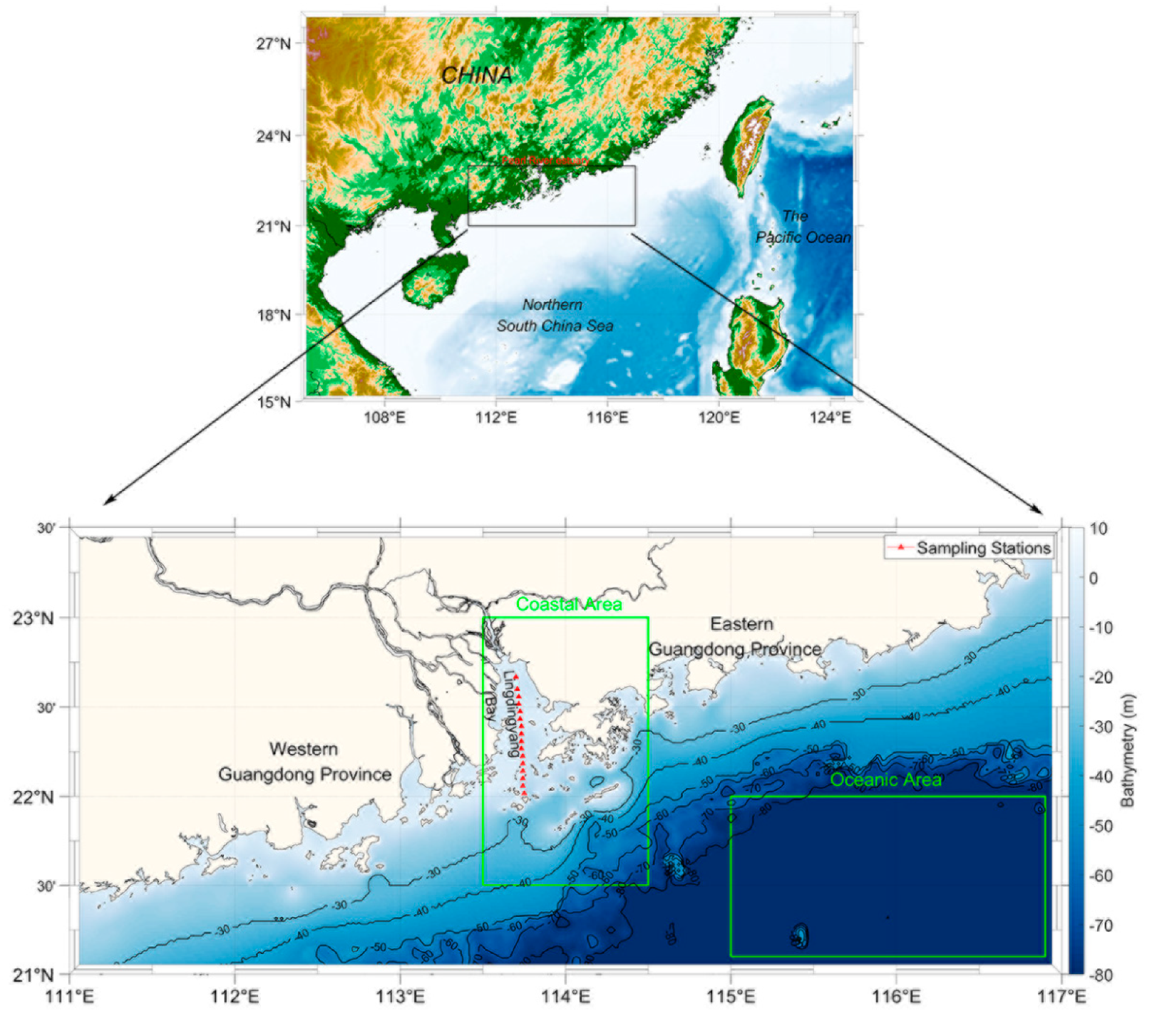
The PRE is located in the northern South China Sea (NSCS), known as a subtropical and high biological productivity estuary. The PRE is characterized by a complicated hydrodynamic system regulated by many physical factors, including bottom topography, river discharge, wind field, and a coastal current [14]. The PRE is influenced by the East Asia monsoon system, characterized by prevailing northeasterly and southwesterly winds in winter and summer, respectively [15,16]. In this study, season refers to those for the northern hemisphere, for example, summer refers to June, July, and August. As China’s third largest river, the Pearl River flows into the PRE through eight main outlets [17], carrying a large amount of organic and inorganic suspended matter, with an annual average discharge of 105 m3·s−1 [18]. With increasing human activity, the PRE is contaminated by industrial pollution, agricultural runoff, and domestic sewage [19,20].
2.2. Data Sources and Processing
2.2.1. In Situ Measurements
A cruise was conducted on 5 June 2012 to collect water samples and the water spectrum. Positions for all sampling stations are plotted in Figure 1. The field spectral measurements were composed of two parts: the above-water remote sensing reflectance (Rrs) and the downwelling irradiance within the water column. To obtain the background water column conditions, water samples from the 15 sampling stations were used for measurement of chlorophyll-a (Cchla), total suspended sediment (Ctsm), absorption coefficient for phytoplankton (ap(λ)), and colored dissolved organic matter (CDOM, ag(λ)) (Table 1).
The above-water Rrs was measured using a spectroradiometer (USB4000, Ocean Optics, Inc., Dunedin, FL, USA) following the National Aeronautics and Space Administration (NASA) ocean-optics standard protocol [21]. The upward radiance (Lu), downward sky radiance (Lsky), and radiance from standard spectra on a reference plaque (Lpla) were measured, and Rrs was calculated using the following equation:
where λ is the wavelength, ρpla is the reflectance of the plaque provided by the manufacturer (Ocean Optics, Inc., Dunedin, FL, USA), ρf is the water surface Fresnel reflectance, where a value of 0.028 was taken for wind speeds of less than 5 m·s−1.
To evaluate the MODIS-based Kd(490) retrieval models, in situ Rrs was aggregated to simulate MODIS/Aqua Rrs according to the following equation [22,23,24]:
where Rrs(Bi) denotes the simulated Rrs for the ith band of MODIS/Aqua, with integration from λm to λn; Rrs_meas(λ) denotes the field-measured Rrs(λ); and RSR(λ) denotes the MODIS/Aqua spectral response function.
Downwelling irradiance within the water column was measured with a TriOS-RAMES hyperspectral spectroradiometer (TriOS GmbH, Oldenburg, Germany). The spectroradiometer recorded irradiance signal in the range of 320 to 950 nm with a wavelength resolution of 3.3 nm. The TriOS-RAMES instrument was slowly hand-lowered at a stable speed from the surface to a water depth of about 5 m and set to a sampling rate of one sample every five seconds. Meanwhile, a pressure sensor recorded the corresponding depth of water. By releasing the TriOS-RAMES instrument (TriOS GmbH, Oldenburg, Germany) into water twice, two profiles of the downwelling irradiance were collected. The two profiles were averaged to minimize the effect of near-surface wave focusing. The natural logarithm of the measured irradiance was plotted against depth, and an estimate of Kd(λ) was acquired from the resulting slope [25]:
where λ is the wavelength, Ed(z) is the downwelling irradiance at depth z, and Δz is the infinitesimal thickness at depth z.
2.2.2. MODIS/Aqua Imagery
The Level-1B MODIS/Aqua ocean color dataset and the geolocation dataset from 2003 to 2017 were obtained from the Level-1 and Atmosphere Archive and Distribution System (LAADS) Distributed Active Archive Center (DAAC). Imagery was preprocessed using the SeaWiFS data analysis system (SeaDAS, version 7.5.1). The Management Unit of the North Seas Mathematical Models (MUMM)-based atmospheric correction [26] and an iterative f/Q Bidirectional Reflectance Distribution Function (BRDF) correction [27,28,29,30] were used to acquire accurate Rrs values. Flags were used to mask contamination from land, clouds, sun glint, and other potential disturbances to the radiance signal.
2.2.3. Ancillary Data
The wind field dataset was obtained from the National Centers for Environmental Prediction (NCEP) Climate Forecast System Version 2 (CFSv2). The model is fully coupled, representing the Earth’s atmosphere, oceans, land, and sea ice [31]. The mixed layer depth (MLD), defined as the depth where the density is equal to the sea surface density plus an increase in density equivalent to 0.8 °C, was acquired from the global ocean Argo gridded dataset (BOA_Argo, provided by the China Argo Real-time Data Center, ftp://data.argo.org.cn/pub/ARGO/BOA_Argo/) [32]. The monthly river runoff was acquired from the Chinese River Sediment Bulletin. The Level-3 MODIS/Aqua sea surface temperature (SST) dataset was obtained from the Ocean Color Website (https://oceancolor.gsfc.nasa.gov/l3/), a website that provides the derived geophysical variables that have been aggregated/projected onto a well-defined spatial grid during a well-defined time period.
2.2.4. Models for Kd(490) Retrieval
At present, the standard methods for Kd(490) estimation are roughly classified into three types: (1) empirical relationship between Kd(490) and apparent optical properties (AOP), including water-leaving radiance or reflectance [11,33,34]; (2) empirical relationship between Kd(490) and chlorophyll-a based on regression analyses [35]; and (3) semianalytical approaches based on radiative transfer models [1,36]. These three types of models, six models in total (Table 2), were evaluated in the PRE waters using the in situ dataset.
2.2.5. S-EOF and Grey Relational Analyses
The S-EOF analysis, proposed by Wang and An (2005) [37], was applied here to detect the spatial patterns and temporal variability of Kd(490) in different seasons. The processing steps of S-EOF analysis are as follows: Firstly, the time series of seasonal Kd(490) anomaly was calculated. Secondly, the EOF was analyzed based on the matrix composed of the four seasons. Finally, each S-EOF mode containing four spatial modes, which represented the spatial patterns of Kd(490) in the four seasons, and a corresponding principal component time series were obtained.
GRA is an important part of grey system theory, which is used to determine the relational degree among factors according to the similarities in their geometry [38]. The GRA was applied here to identify the dominant water constituents (total suspended matter, phytoplankton, and dissolved matter) affecting the spatial distribution and temporal variation of Kd(490). In GRA, the reference series of Kd(490) and comparison sequences (water constituents, including Ctsm, Cchla, and adg(443)) were constructed in advance to calculate the grey relational grade (GRG), which is a measure of similarity between the reference sequence and comparison sequences. Details about the calculation of GRG were described by Liu and Lin (2005) [39] and Wan et al. (2019) [40].
2.2.6. Performance Assessment
To compare the performance of different Kd(490) retrieval models, several statistical parameters were used: the determination coefficient (R2), root mean square error (RMSE), mean absolute difference (MAD), and mean absolute percentage difference (MAPD), which are calculated as:
where xm and xp denote the measured and predicted samples, respectively; denotes the mean value of the measured samples; and N is the number of samples.
3. Results
3.1. Model Performance
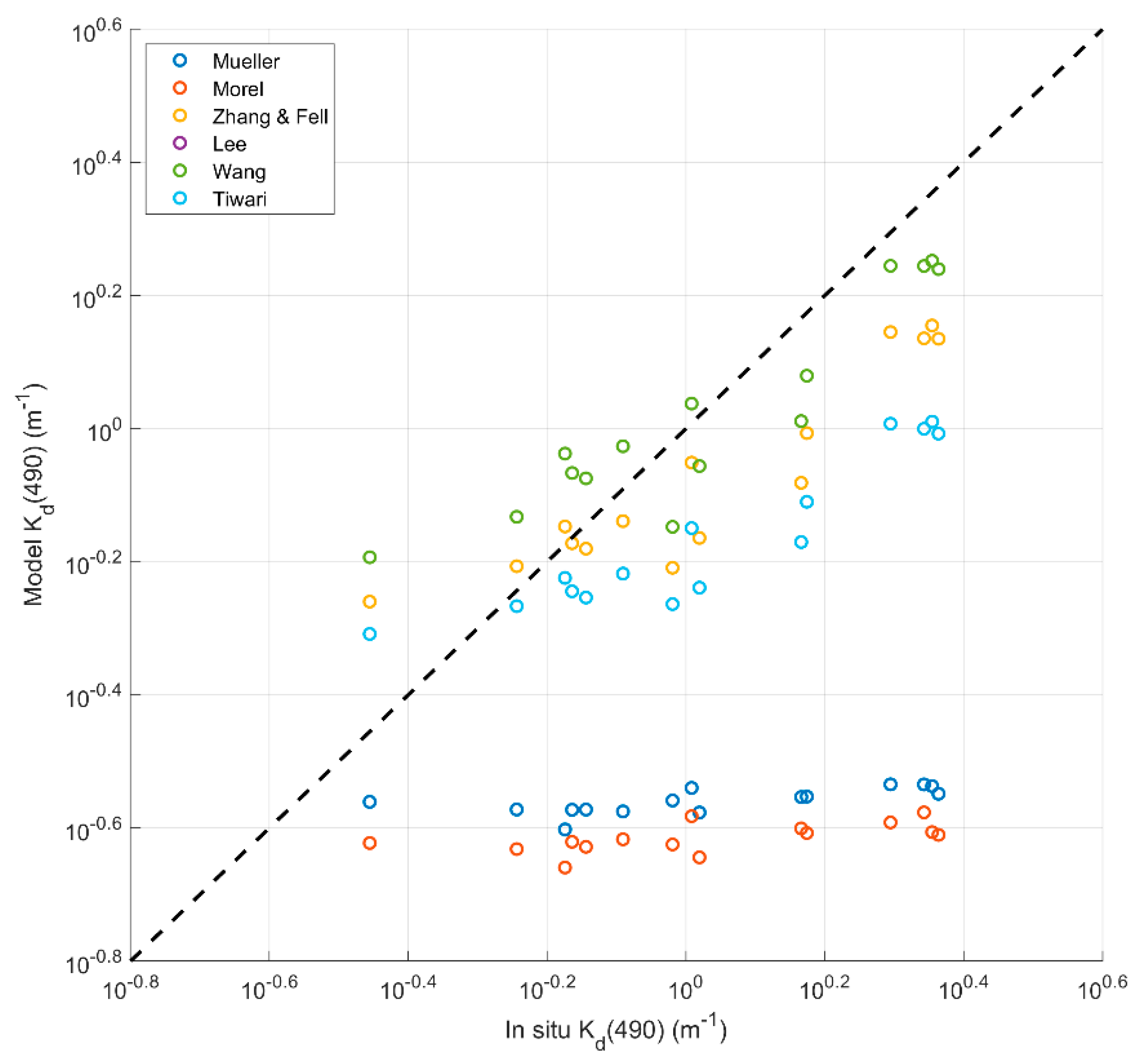
We evaluated the six different models with MODIS/Aqua spectral bands or Cchla. The evaluation was based on the comparison of the model-derived Kd(490) with in situ measured Kd(490) collected from the PRE on 5 June 2012. Figure 2 shows scatterplots between the in situ measured and different models’ Kd(490) retrievals, and Table 3 lists the statistical parameters. The results provided by both Mueller’s and Morel’s models constantly underestimated the Kd(490) compared with the in situ dataset for the PRE, with RMSEs higher than 1.1 m−1, MADs close to 1.0 m−1, and MAPDs up to 70%. The Morel (empirical model with Cchla) and Mueller (empirical model with water-leaving radiance) models not only underestimated the in situ values of the PRE, they had little to no sensitivity along a broad gradient of in situ values.
By comparison, the other four models appeared to be more effective when applied in the PRE waters. These four models performed well with R2 values higher than 0.9, RMSEs ranging from 0.31 to 0.70 m−1, MADs ranging from 0.27 to 0.54 m−1, and MAPDs ranging between 25.51% and 37.10%. We found that Wang’s model, combining Lee’s algorithm for turbid waters and Mueller’s algorithm for clear waters, was a better choice for Kd(490) retrieval in the PRE waters. Comparison of Wang’s model to the other models showed that Wang’s model had considerably lower RMSE and MAD values and outperformed the other models, especially at relatively higher Kd(490) levels.
3.2. Spatial Distribution and Temporal Variation
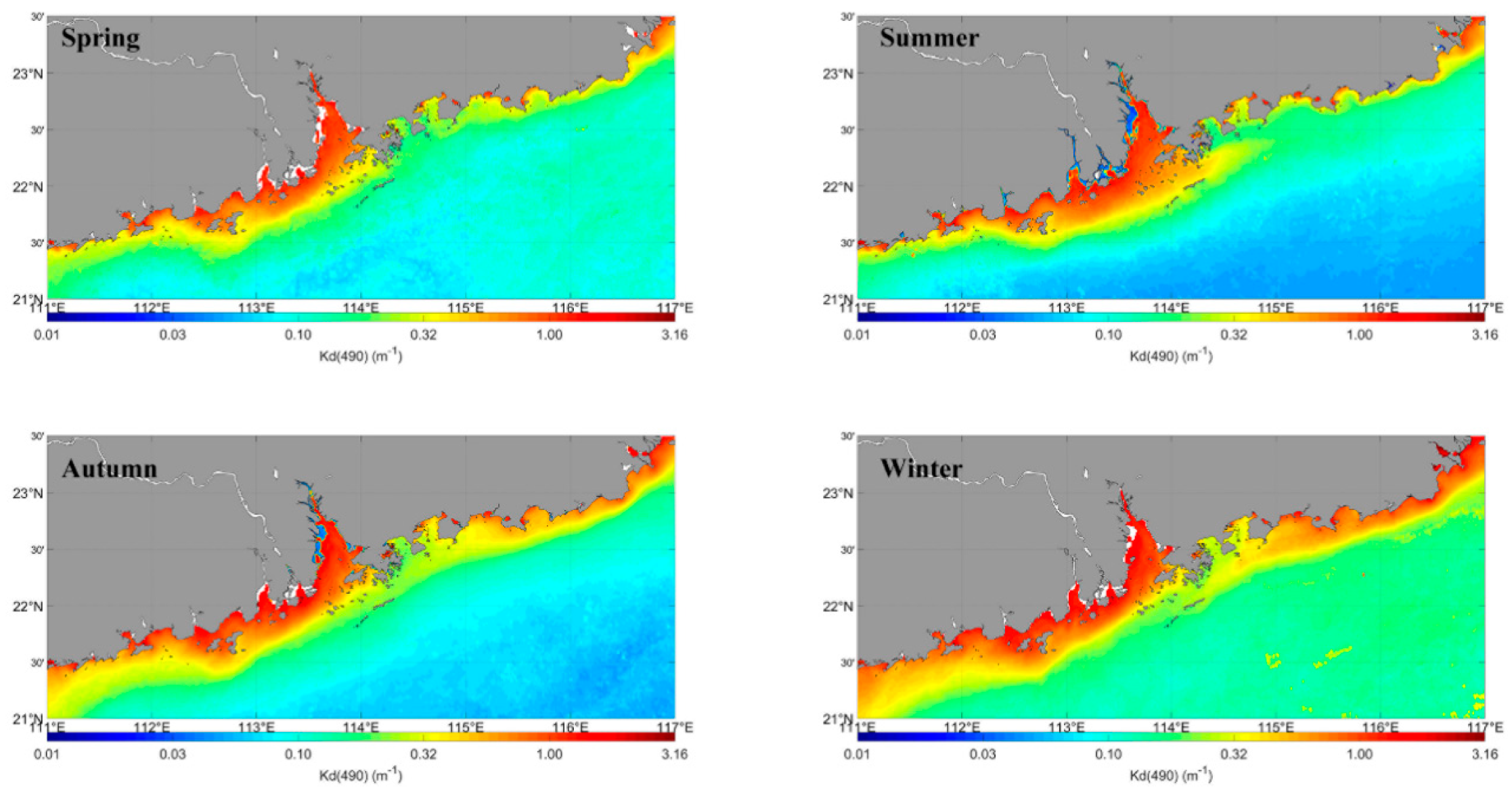
Given its superior performance of the six considered models, the long-term MODIS Kd(490) products were derived based on Wang’s model. Significant seasonal variation was identified over the entire study area from 2003 to 2017 (Figure 3). The mean values for the entire study area were 0.13 m−1 in spring, 0.12 m−1 in summer, 0.14 m−1 in autumn, and 0.21 m−1 in winter. In the coastal area, the relatively high Kd(490) was observed in Lingdingyang Bay (LB) and western Guangdong Province (GDP), where the highest value exceeded 4.0 m−1. In summer, the river plume extends from LB southeastward into the coastal region, resulting in a wider distribution of high-value Kd(490). The plume waters formed a tongue along the eastern GDP (located 113–115°E, 22–22.5°N) in some specific years, though this feature was not so remarkable in the seasonal climatological imagery due to long-term average smoothing. The influence of the terrestrial input of nutrients from the Pearl River is highest in summer. In addition, a southeast wind prevails and rainfall mainly occurs in summer. The winds blow from PRE to the middle shelf. The winds control the spatial pattern of Kd(490) distribution in the PRE. In the eastern GDP, relatively higher Kd(490) values were found in autumn and winter, whereas lower values were observed in spring and summer. This phenomenon is closely correlated with the coastal upwelling along the eastern GDP coast [41,42]. Chen et al. (1982) [43] reported that a radiating current could generate an upwelling in winter near the Jieshi Bay in the eastern GDP. In open ocean areas, the average Kd(490) values in winter and spring were higher than that in summer and autumn. The prevailing northeasterly monsoon is stronger in the northern South China Sea in winter, so the MLD was deeper. The mixing effects are relatively stronger in winter. Figure 3 shows that the distribution of Kd(490) reveals the significant seasonal variation over the entire study area during 2003 to 2017.
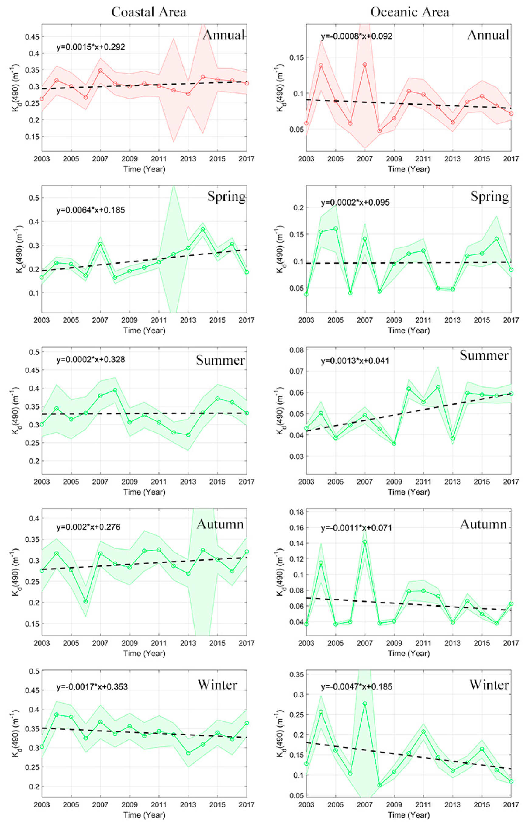
Due to the different physical factors affecting the variability of Kd(490) in nearshore and offshore regions, we separated the two regions and analyzed the separate regions’ trends rather than averaging the entire region for time series analysis (Figure 4). Two subregions, representing the turbid coastal waters and the clear open ocean waters, were chosen (marked in Figure 1 by green boxes). During the period from 2003 to 2017, the trend lines of the annual average in coastal and oceanic areas were around 0.3 and 0.1 m−1, respectively. No significant increasing or decreasing trend was observed. However, in terms of seasonal variability, the average nearshore and offshore Kd(490) showed some differences. The average Kd(490) in the coastal area was constantly high in the four seasons, with values ranging between 0.2 and 0.4 m−1. An increasing trend was observed in spring, with a slope of approximately 0.006 m−1 per year. Compared to the coastal region, significant seasonal variability was observed in the open ocean region. Average Kd(490) values during spring and winter were found to be higher than during summer and autumn. Trend lines of spring and winter ranged from 0.1 to 0.2 m−1, whereas those in summer and autumn ranged from 0.04 to 0.08 m−1. In winter, the average showed a significant decreasing trend, with a slope of approximately −0.005 m−1 per year.
3.3. GRG of Water Constituents
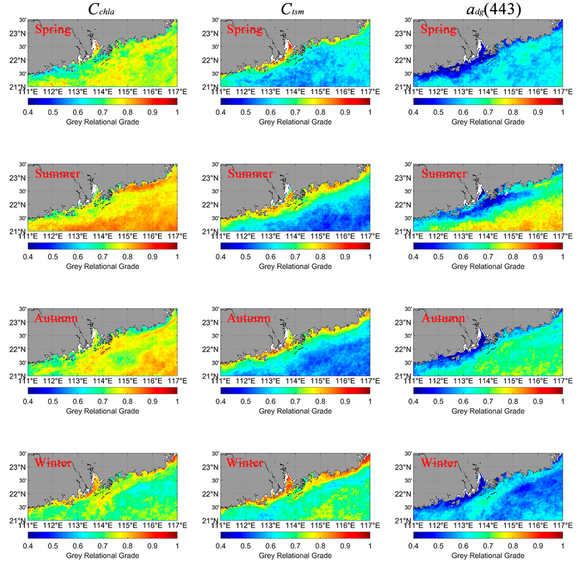
The optical properties were determined using the absorption or backscattering of different water constituents. Here, three types of water constituents were considered; the monthly average Ctsm, Cchla, and adg(443) were obtained based on the same atmospheric-corrected MODIS/Aqua Rrs dataset that was used for Kd(490) retrieval. A band ratio algorithm was adopted for Ctsm retrieval [17]. The OC3M algorithm was used for Cchla retrieval [44]. The generalized inherent optical property (GIOP) model was applied for adg(443) retrieval [45,46]. The GRGs, which can be used to measure the relationships between the Kd(490) and the three water constituents, were calculated pixel by pixel for the four seasons (Figure 5).
Spatially, GRGs between Kd(490) and Cchla or adg(443) were higher in the clear open ocean region than in the coastal region, but the values contrasted between Kd(490) and Ctsm. The GRGs gradually decreased from nearshore to offshore, similar to the distribution of Ctsm. Seasonally, the GRG was higher in summer and autumn than in spring and winter between Kd(490) and Cchla, with most of the pixels’ values being above 0.8. Similar phenomena were observed in the GRGs between Kd(490) and adg(443), although the average value was lower than between Kd(490) and Cchla.
3.4. S-EOF Analysis
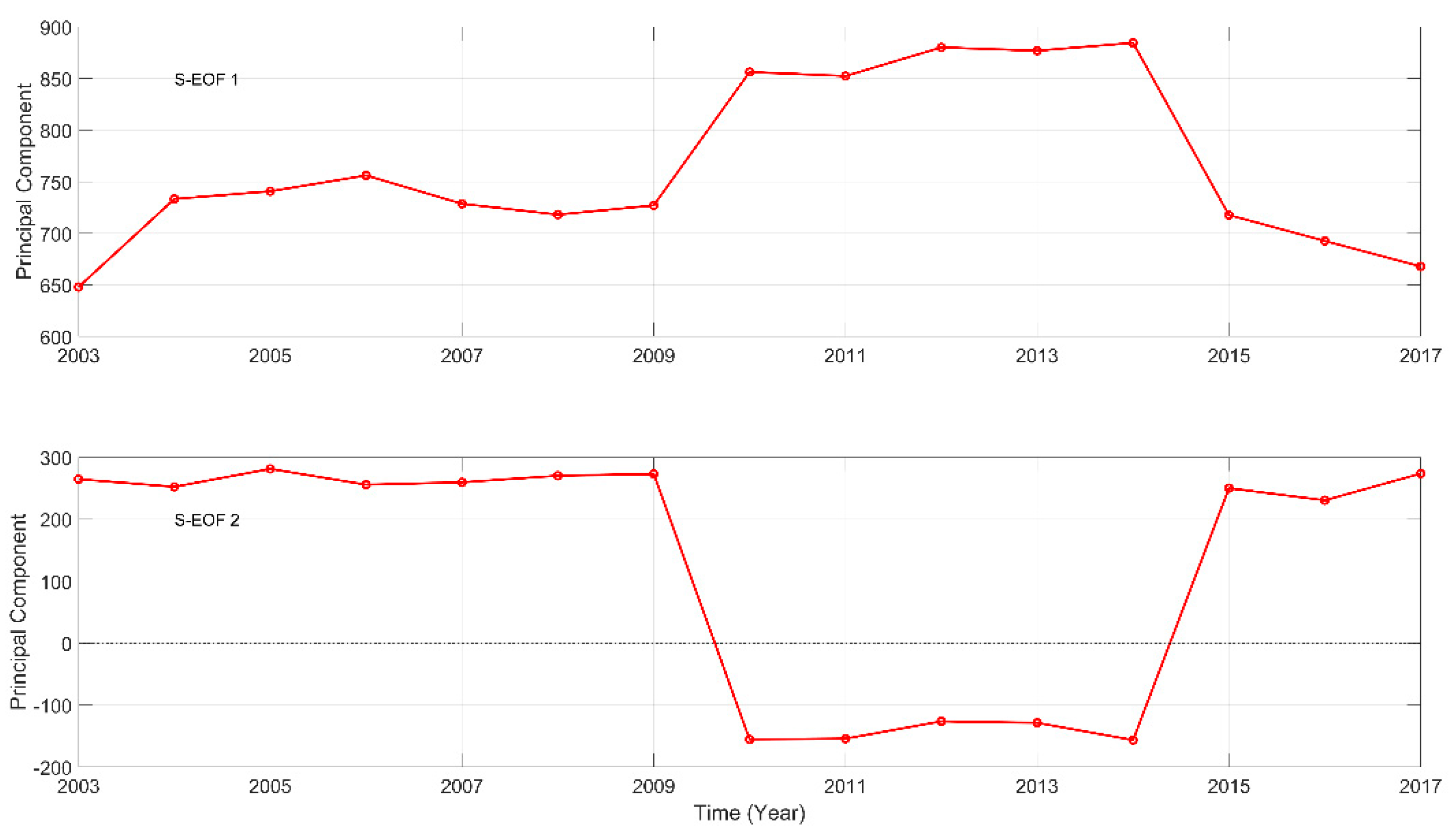
An S-EOF analysis was performed after subtracting the long-term monthly climatological average Kd(490). The first two modes and the corresponding principal components (PC) were separated, which accounted for approximately 81.16% of the total variance (Table 4).
Figure 6 shows the PC time series of the first two S-EOF modes. All the values of PC1 were positive, indicating that the seasonal fluctuation was stable. The strength of fluctuation was related to the magnitude of the positive values. We observed a significant increasing trend during 2003 to 2006, whereas a slight decline was observed during 2007 to 2009. From the beginning of 2010 to 2014, PC1 reached its highest value. After that, the values began to decline again. PC2 was characterized by negative values during 2010 to 2014 and positive values in other years.
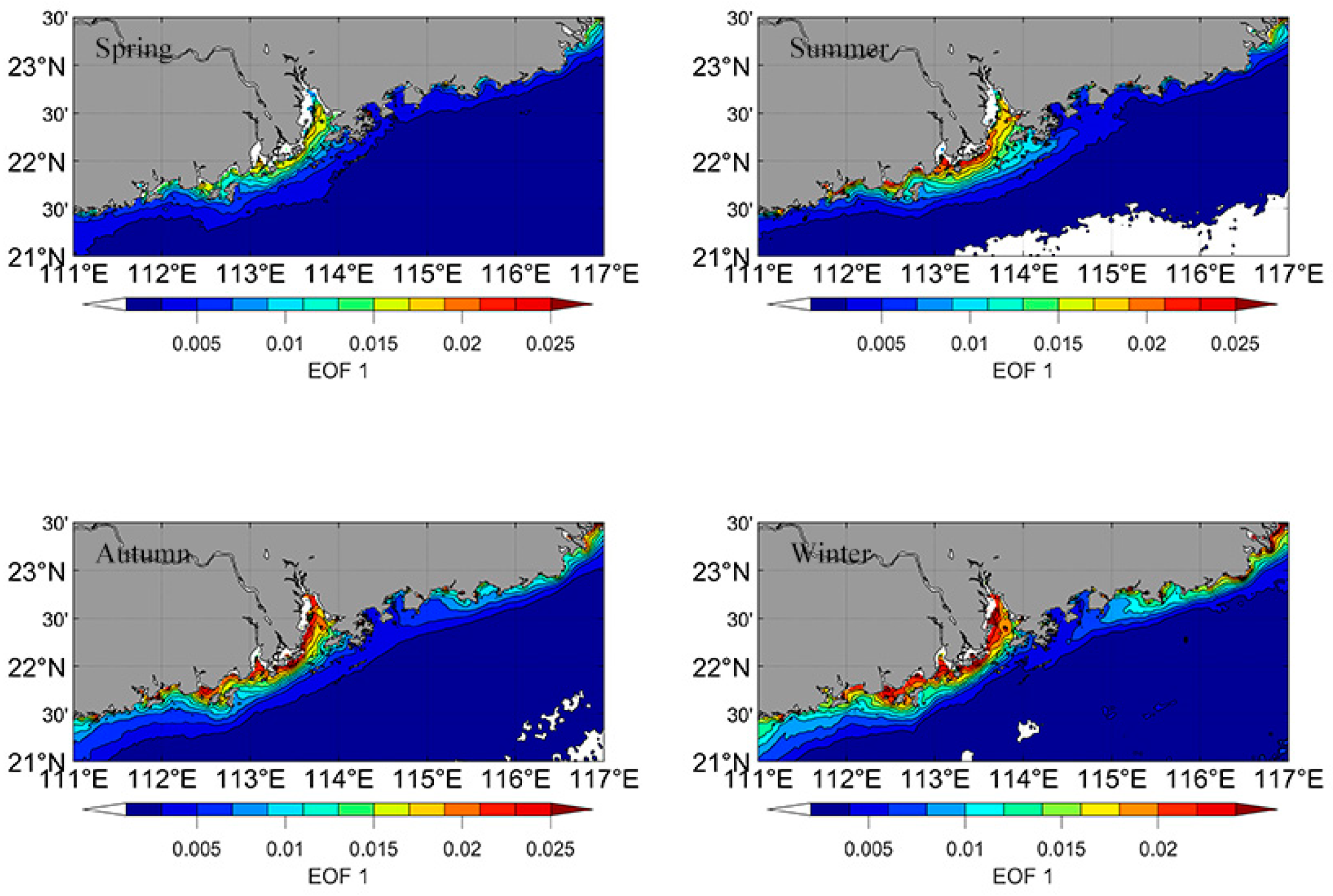
Figure 7 shows the spatial distribution of the first mode of S-EOF, which explained approximately 56.7% of the total variance. Relatively high values were observed in LB and the western coast of GDP in the four seasons, and the average values for spring were significantly lower than in the other seasons. In summer, the high value area tended to expand to the southeastern LB. From autumn to winter, we observed a high value area along the east coast of the GDP, whereas this high value area disappeared in spring and summer.
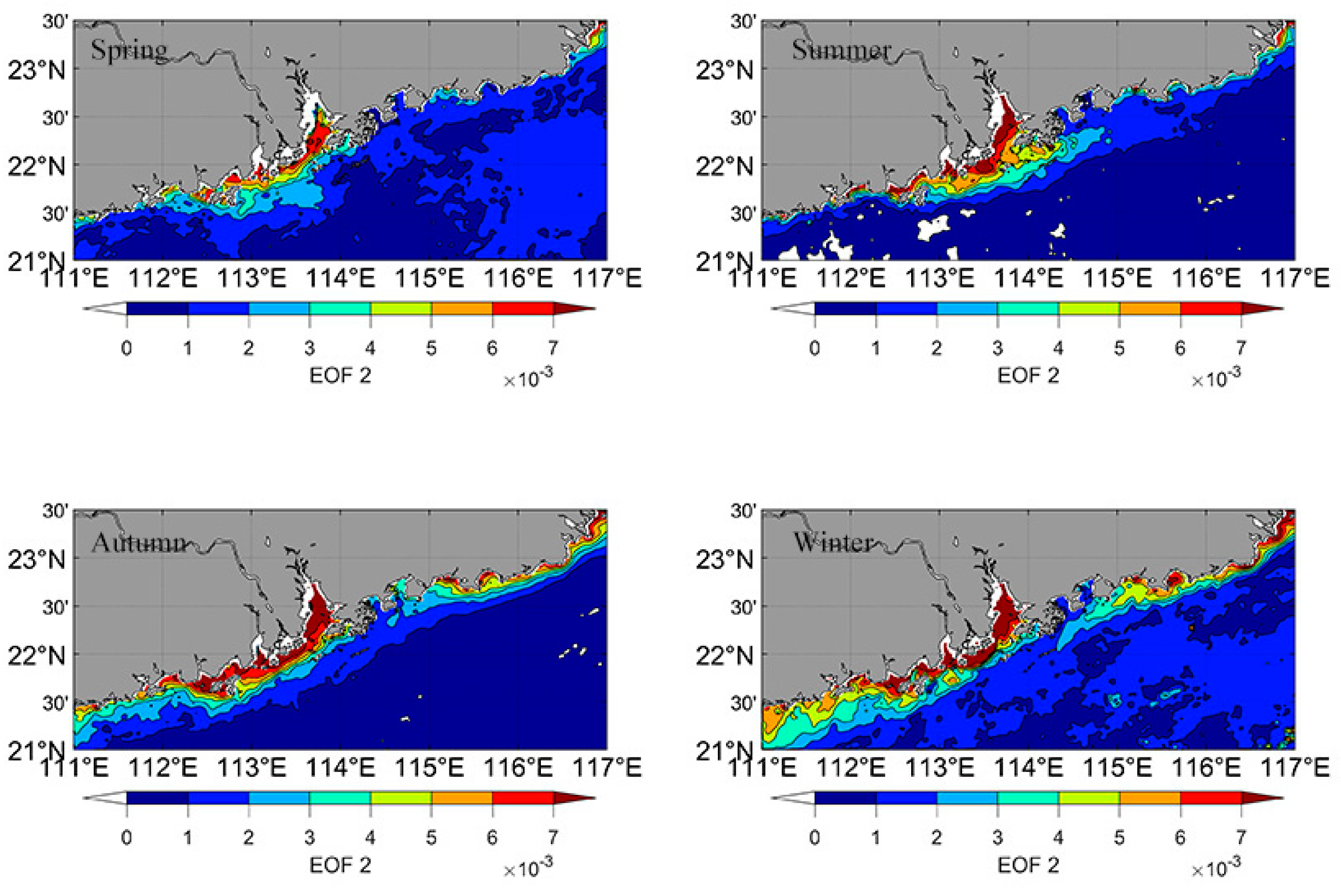
The second mode of S-EOF explained 24.5% of the total variance. A relatively higher value area was observed in LB during the four seasons (Figure 8). In summer, the high value area extended eastward and formed a distinguishable tongue. Compared with spring and summer, higher values were observed along the whole coastal zone of the PRE. Based on the second mode of S-EOF, we found that the higher values in the eastern GDP extended westward and formed a distinguishable tongue in winter.
4. Discussion
4.1. Evaluation of Kd(490) Models
Both Mueller and Morel’s models were unsuitable for the PRE waters because these two models were established for clear waters and only use the spectral information from the blue and green bands. For clear waters where the downwelling attenuation is mainly determined by phytoplankton, the blue–green band ratio is sensitive to the variability of the Cchla, resulting in a high accuracy for Kd(490) retrieval. However, for turbid waters where the optical properties are more complex, the blue–green band ratio demonstrates a lower sensitivity to the variability in Kd(490). The strong absorption of phytoplankton and CDOM could lead to relatively smaller Rrs in the blue and green bands [47,48]. In the PRE, the water constituents are from river inputs and coastal erosion. The Cchla, CDOM, and Ctsm are very high, which may result in both Mueller and Morel’s models being inapplicable in the PRE.
Tiwari’s model uses the reflectance ratio at 490 and 670 nm, Rrs(490)/Rrs(670), to derive Kd(490). Zhang’s model is composed of two independent algorithms: one based on the ratio Rrs(490)/Rrs(555) for clear waters and another based on the ratio Rrs(490)/Rrs(665) for turbid waters. When tested with the independent PRE dataset, the predictions of these two models were statistically better compared to both Mueller’s and Morel’s models. However, the two models also showed a pronounced underestimation for higher Kd(490) values (>1.0 m−1), which might be due to the strong backscattering of suspended sediments in the more turbid waters in the PRE. Lee’s model produced a suitable estimation, which uses a relationship relating the backscattering coefficient at 490 nm to the irradiance reflectance just beneath the surface within the red band. The performance of Wang’s model was the same as Lee’s, which was attributed to the same approach used in both models for highly turbid waters. In Wang’s model, the retrieval method switched to Mueller’s in clear waters, and the bridging of the two types of models is based on a certain weighting function (W). The spectral information within the red band cannot be ignored when retrieving Kd(490) for turbid waters. However the values of Rrs(670)/Rrs(490) tended to be very low and, therefore, values of Kd(490) for clear waters were inaccurate. Therefore, Wang’s model, which uses a combination of different algorithms for clear and turbid waters, is a better choice for Kd(490) retrieval in the PRE waters.
4.2. Dominant Contributor to Kd(490) of Water Constituents
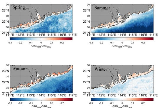
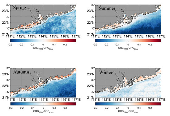
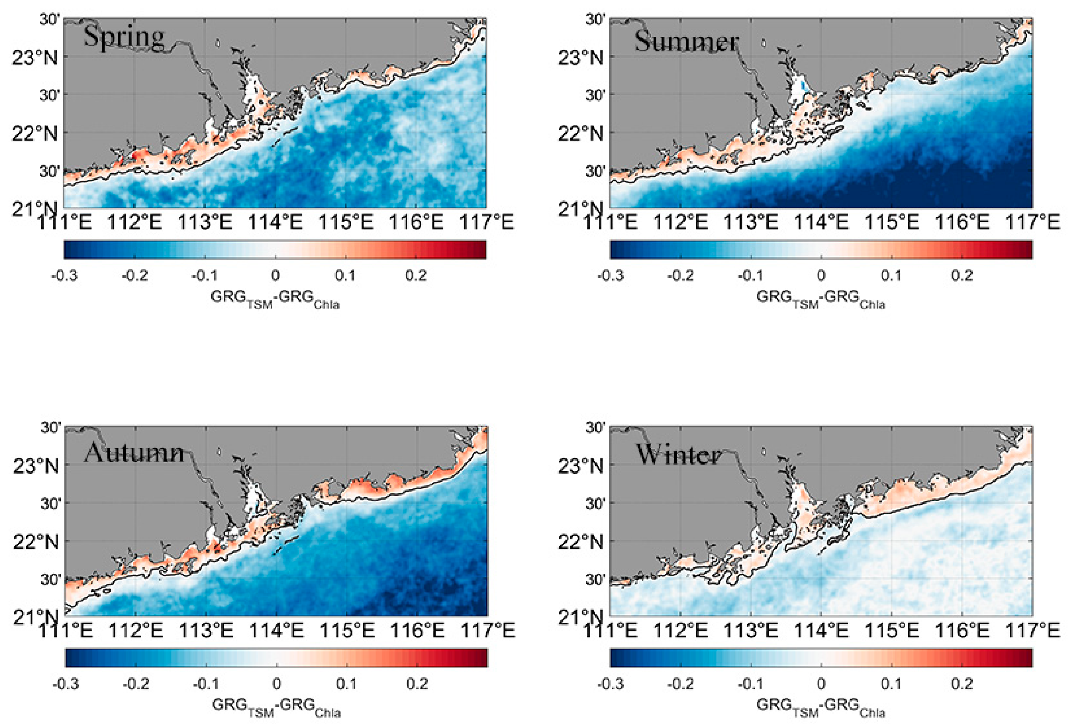
Attenuation of light in water depends on concentrations of particulate matter and dissolved matter, which can be expressed by Ctsm, Cchla, and the absorption coefficient of CDOM [7,49]. The contribution of these constituents varies for different types of water and within the same water body in different seasons [50,51,52]. Since the calculated GRGs between Kd(490) and adg(443) were significantly lower than the other two water constituents, only the GRGs of Ctsm and Cchla were considered. Figure 9 depicts the subtraction of both GRGs. Positive values indicate the GRGs of Ctsm were higher than those of Cchla, which means that Ctsm played a dominant role in Kd(490) variability. In contrast, negative values indicate that the Cchla had a greater influence. The Ctsm-dominated were waters generally located in coastal and estuarine turbid areas, whereas the Cchla-dominated waters were observed in open clear ocean. Notably, waters dominated by adg(443) were rare. The strong absorption of CDOM in the blue bands influenced the variability of Kd(490), particularly in waters with high CDOM concentrations. The major sources of CDOM in the PRE were the river water and the human and industrial sewage [53,54]. However, in coastal or estuarine areas with highly turbid waters, Ctsm can reach over 100 g˖m−3. During the survey conducted on 5 June 2012, the range of measured ag(443) was 0.12 to 0.58 and the range of measured ap(443) was 0.31 to 1.61. The latter was approximately three orders higher than the former, indicating that the influence of total suspended sediments on Kd(490) was far greater than that of CDOM.
The distribution of dominant constituents showed some seasonality. In spring and summer, the Ctsm-dominated waters were mainly distributed in LB and the western GDP. The Ctsm-dominated area was confined close to the nearshore areas in the eastern GDP, indicating the impact of Cchla can extend from offshore to nearshore regions. Compared with other seasons, the most significant feature in summer was the southward extension of Ctsm from LB to the open ocean, which can probably be attributed to the increase in river runoff. In autumn and winter, the Ctsm-dominated area was wider in the eastern GDP than in spring and summer. The underlying reason for the change in area still requires future research. Currently, the change in area in the eastern GDP during autumn and winter might be indirectly caused by the decrease in Cchla rather than the variability of Ctsm. In autumn and winter, the entire eastern GDP is influenced by monsoons. The northeasterly wind-induced downwelling appears to decrease the amount of resuspension, resulting in the slight decrease in surface Ctsm, which seems to contradict the expansion of the Ctsm-dominated area. However, the downwelling also inhibits the growth of phytoplankton. The decrease in surface Cchla may prevent it from becoming the primary factor affecting the variability of Kd(490).
4.3. Influence of Physical Factors on Kd(490) Variability
Figure 3 shows that the Kd(490) values in the PRE waters were markedly different in different regions and in different seasons, and Figure 9 shows that the spatial variations can be attributed to the changes in Cchla and Ctsm.
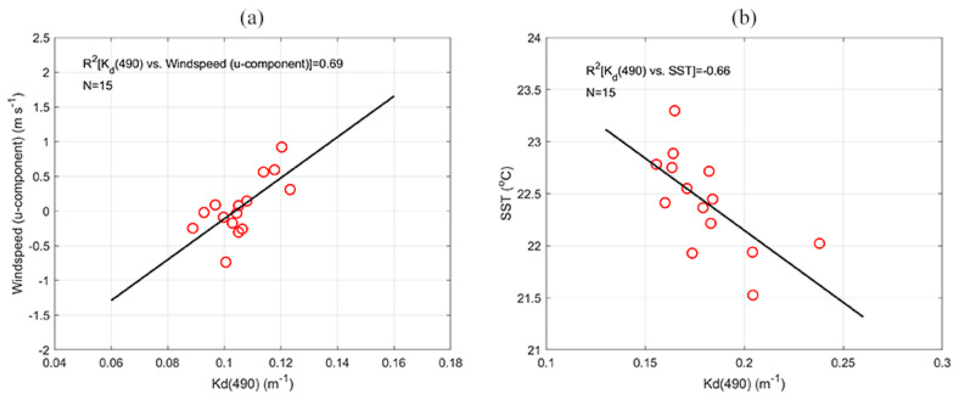
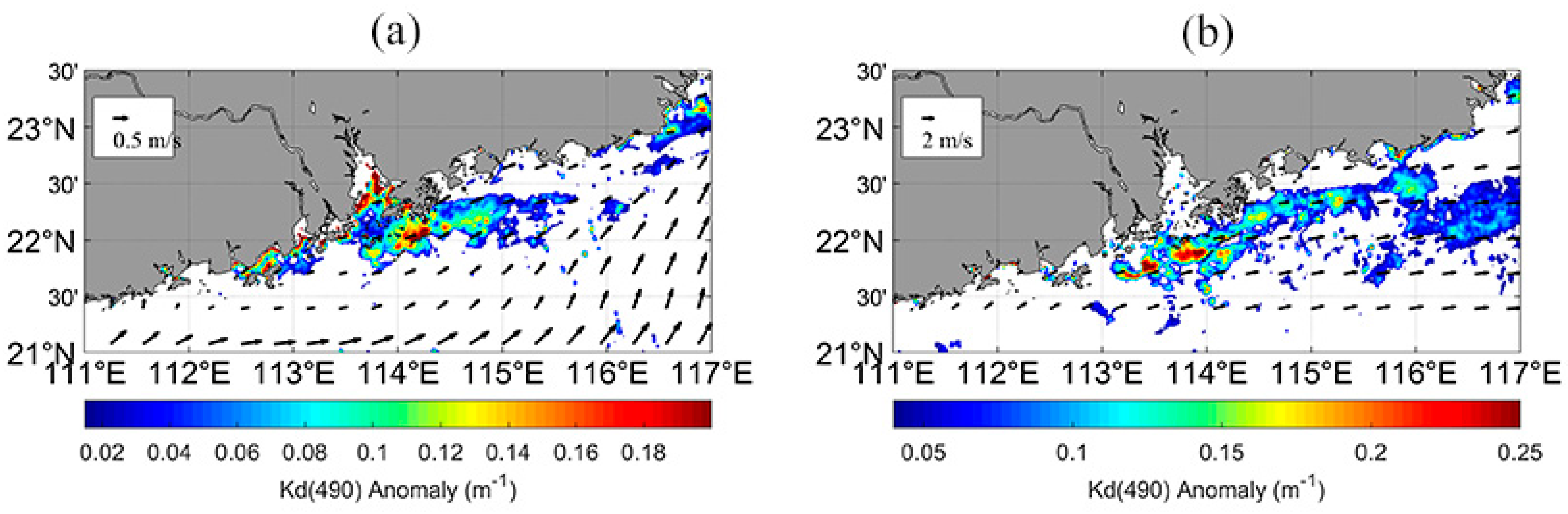
To understand the mechanism through which the seasonal Kd(490) varies, correlation analysis was performed between several types of physical factors, including wind field, river runoff, MLD, SST, and seasonal average Kd(490). The results showed that the average Kd(490) was highly correlated with the wind speed (u-component) in summer, with an R2 of about 0.69. During winter, we found a significant negative correlation between Kd(490) and SST, with an R2 of –0.66 (Figure 10). Seasonal anomalies were also obtained by subtracting the seasonal climatological average. In 2007 and 2015, when the wind speed anomaly (u-component) reached its peak, a distinguishing tongue of Kd(490) anomaly was observed near the southeastern LB (Figure 11). Inside this tongue region, the Kd(490) anomaly in the west was higher than in the east, indicating that the variability can be attributed to the high turbid river plume waters in the surface layer, which are driven by the intense eastward wind.
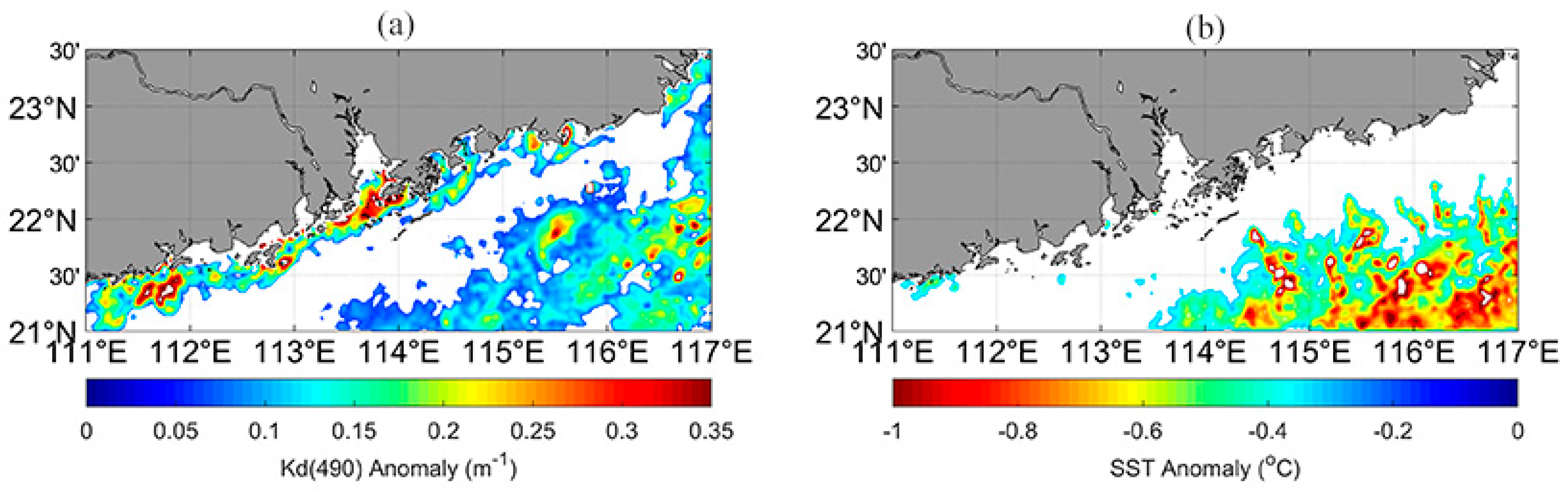
The winter SST cooling in 2004 was the most significant during the whole study period, and was located in the southeastern PRE, which was about 0.4 °C cooler than the winter climatological average. Within these cooling regions, Kd(490) values higher than the average values were observed, with anomalies ranging approximately from 0.1 to 0.35 m−1. The observed winter variations in Kd(490) in the southeastern PRE were strongly consistent with the changes in SST anomalies, and higher values coincided with lower SST (Figure 12).
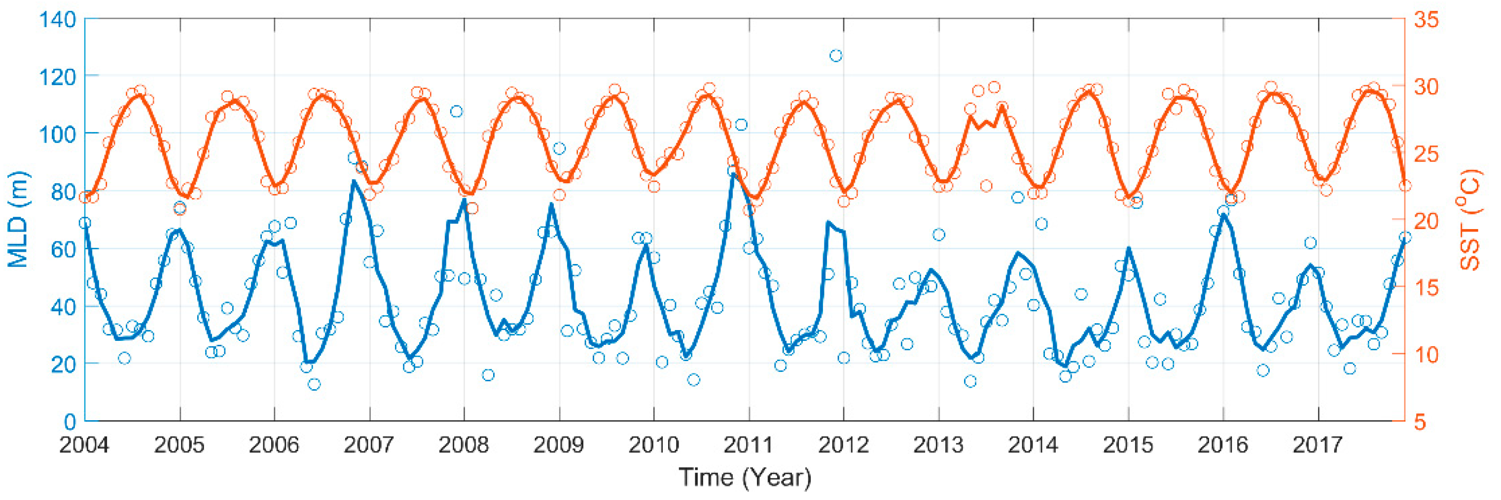
The variability of Kd(490) in the southeastern PRE was mainly determined by Cchla. The average values of Kd(490) were higher in winter than in summer. This seasonal variability might be attributed to the deepening of MLD in winter. In marine systems, MLD is generally deeper in winter than in summer [55]. Nutrients are brought from the bottom of the ocean to the surface or subsurface, which may enhance phytoplankton growth. The strong mixing in winter was demonstrated by the deepening of MLD, and a significant relationship between SST and MLD provided evidence that nutrients were supplied from the bottom waters (Figure 13).
5. Conclusions
Accurate estimation of Kd(490) using ocean color remote sensing imagery is challenging in turbid coastal waters due to the optical complexity of the water. Several approaches, including empirical and semianalytical models, were applied to retrieve the Kd(490) in PRE water. The results showed that Wang’s model was more accurate and is most suitable for PRE water, which uses a combination of different algorithms for clear and turbid waters. Hence, Wang’s model was selected for deriving Kd(490) products from long-term MODIS/Aqua imagery.
Derived from long-term MODIS/Aqua imagery, the temporal variability and spatial distribution of Kd(490) were tracked using S-EOF analysis. The results of GRA showed that both phytoplankton and suspended sediments were the two dominant contributors to the variability in Kd(490). The Ctsm-dominated waters were generally located in coastal and estuarine turbid area, whereas the Cchla-dominated waters were observed in clear open ocean. The influence of wind field on the variability of Kd(490) was significant near the coastal and estuarine regions in summer. With the strengthening of the eastward wind, a water tongue of relatively higher Kd(490) values formed in the southeastern PRE. In winter, the location of the negative SST anomaly and positive Kd(490) anomaly was strongly consistent, indicating that the sea surface cooling was related to the positive Kd(490) anomaly. The winter variability might be attributed to the strong mixing, which brought nutrients from the bottom layer to the surface to enhance phytoplankton growth.
Estuarine and coastal regions are complex ecosystems. To better examine the biogeochemical responses to physical events, a combination of remote sensing and coupled hydrodynamic–biological models should be applied in future research.
Author Contributions
Conceptualization, S.T. and H.Y.; implementation, H.Y. and C.Y.; validation, H.Y. and C.Y.; writing—original draft preparation, H.Y. and C.Y.; writing—review and editing, S.T., H.Y., and C.Y.; funding acquisition: S.T. All authors have read and agreed to the published version of the manuscript.
Funding
This research was funded by the Strategic Priority Research Program of the Chinese Academy of Sciences (No. XDA13010404 and XDA19060501), the Key Special Project for Introduced Talents Team of Southern Marine Science and Engineering Guangdong Laboratory (Guangzhou) (No. GML2019ZD0302, 2019BT2H594), the National Key Research and Development Program of China (No. 2018YFD0900901), the Joint Funds of the National Natural Science Foundation of China (No. U1901215), and Key Research and Development Project of GuangXi (GUI-KE: AB16380339).
Acknowledgments
The authors would like to thank the NASA Goddard Space Center for providing MODIS data and the NASA OBPG group for providing the SeaDAS software package. Our colleagues in the Ocean Color group of the South China Sea Institute of Oceanology, Chinese Academy of Sciences, are thanked for their effort in collecting and processing the samples.
Conflicts of Interest
The authors declare no conflict of interest.
References
- Wang, M.; Son, S.H.; Harding, L.W., Jr. Retrieval of diffuse attenuation coefficient in the Chesapeake Bay and turbid ocean regions for satellite ocean color applications. J. Geophys. Res. 2009, 114. [Google Scholar] [CrossRef]
- Zhang, Y.; Liu, X.; Yin, Y.; Wang, M.; Qin, B. A simple optical model to estimate diffuse attenuation coefficient of photosynthetically active radiation in an extremely turbid lake from surface reflectance. Opt. Express 2012, 20, 20482–20493. [Google Scholar] [CrossRef] [PubMed]
- Robert, P.B.; Alexander, S.; Kirill, Y.K. Optical Properties and Remote Sensing of Inland and Coastal Waters, 1st ed.; CRC Press: New York, NY, USA, 1995. [Google Scholar]
- Zhao, J.; Barnes, B.; Melo, N.; English, D.; Lapointe, B.; Muller-Karger, F.; Schaeffer, B.; Hu, C.M. Assessment of satellite-drived diffuse attenuation coefficients and euphotic depths in south Florida coastal waters. Remote Sens. Environ. 2013, 131, 38–50. [Google Scholar] [CrossRef]
- Wu, Y.; Tang, C.C.; Sathyendranath, S.; Platt, T. The impact of bio-optical heating on the properties of the upper ocean: A sensitivity study using a 3-D circulation model for the Labrador Sea. Deep. Sea Res. Part II Top. Stud. Oceanogr. 2007, 54, 2630–2642. [Google Scholar] [CrossRef]
- Saulquin, B.; Hamdi, A.; Gohin, F.; Populus, J.; Mangin, A.; D’Andon, O.F. Estimation of the diffuse attenuation coefficient KdPAR using MERIS and application to seabed habitat mapping. Remote Sens. Environ. 2013, 128, 224–233. [Google Scholar] [CrossRef] [Green Version]
- Shi, K.; Zhang, Y.; Liu, X.; Wang, M.; Qin, B. Remote sensing of diffuse attenuation coefficient of photosynthetically active radiation in Lake Taihu using MERIS data. Remote Sens. Environ. 2014, 140, 365–377. [Google Scholar] [CrossRef]
- Jerlov, N.G. Optical Oceanography; Elsevier: New York, NY, USA, 1976. [Google Scholar]
- Clavano, W.; Boss, E.; Karp-Boss, L. Inherent optical properties of non-spherical marine-like particles-From theory to observation. Oceanogr. Mar. Biol. 2007, 45, 1–38. [Google Scholar] [CrossRef]
- McClain, C.R.; Feldman, G.C.; Hooker, S.B. An overview of the SeaWiFS project and strategies for producing a climate research quality global ocean bio-optical time series. Deep. Sea Res. Part II Top. Stud. Oceanogr. 2004, 51, 5–42. [Google Scholar] [CrossRef]
- Mueller, J.L. SeaWiFS Algorithm for the Diffuse Attenuation Coefficient K(490) Using Water-Leaving Radiance at 490 and 555 nm; SeaWiFS Postlaunch Calibration and Validation Analyses, Part 3; Center for Hydro-Optics and Remote Sensing/SDSU: San Diego, CA, USA, 2000; Chapter 3. [Google Scholar]
- Shi, W.; Wang, M. Characterization of global ocean turbidity from Moderate Resolution Imaging Spectroradiometer ocean color observations. J. Geophys. Res. Oceans 2010, 115. [Google Scholar] [CrossRef] [Green Version]
- Kratzer, S.; Brockmann, C.; Moore, G. Using MERIS full resolution data to monitor coastal waters—A case study from Himmerfjärden, a fjord-like bay in the northwestern Baltic Sea. Remote Sens. Environ. 2008, 112, 2284–2300. [Google Scholar] [CrossRef]
- Wong, L.A.; Heinke, G.; Chen, J.C.; Xue, H.; Dong, L.X.; Su, J.L. A model study of the circulation in the Pearl River Estuary (PRE) and its adjacent coastal waters: 1. Simulations and comparison with observations. J. Geophys. Res. Oceans 2003, 108, 3156. [Google Scholar] [CrossRef]
- Wyrtki, K. Physical Oceanography of the Southeast Asian Waters: Scientific Results of Marine Investigations of the South China Sea and the Gulf of Thailand; Naga Report 2; Scripps Institution of Oceanography: San Diego, CA, USA, 1961; 195p. [Google Scholar]
- Gan, J.; Li, H.; Curchitser, E.N.; Haidvogel, D.B. Modeling South China Sea circulation: Response to seasonal forcing regimes. J. Geophys. Res. 2006, 111, C06034. [Google Scholar] [CrossRef]
- Ye, H.; Chen, C.; Tang, S.; Tian, L.; Sun, Z.; Yang, C.; Liu, F. Remote sensing assessment of sediment variation in the Pearl River Estuary induced by Typhoon Vicente. Aquat. Ecosyst. Health Manag. 2014, 17, 271–279. [Google Scholar] [CrossRef]
- Cai, W.J.; Dai, M.H.; Wang, Y.C.; Zhai, W.D.; Huang, T.; Chen, S.T.; Zhang, F.; Chen, Z.Z.; Wang, Z.H. The biogeochemistry of inorganic carbon and nutrients in the Pearl River estuary and the adjacent Northern South China Sea. Cont. Shelf Res. 2004, 24, 1301–1319. [Google Scholar] [CrossRef]
- Chen, C.; Tang, S.; Pan, Z.; Zhan, H.; Larson, M.; Jonsson, L. Remotely sensed assessment of water quality levels in the Pearl River Estuary, China. Mar. Pollut. Bull. 2007, 54, 1267–1272. [Google Scholar] [CrossRef]
- Zhao, J.; Cao, W.; Wang, G.; Yang, D.; Yang, Y.; Sun, Z.; Zhou, W.; Liang, S. The variations in optical properties of CDOM throughout an algal bloom event. Estuar. Coast. Shelf Sci. 2009, 82, 225–232. [Google Scholar] [CrossRef]
- Mueller, J.L.; Fargion, G.S. Ocean Optics Protocols for Satellite Ocean Color Sensor Validation; SeaWiFS Technical Report Series; NASA Center for AeroSpace Information: Linthicum Heights, MD, USA, 2002. [Google Scholar]
- Sun, D.; Hu, C.; Qiu, Z.; Shi, K. Estimating phycocyanin pigment concentration in productive inland waters using Landsat measurements: A case study in Lake Dianchi. Opt. Express 2015, 23, 3055–3074. [Google Scholar] [CrossRef] [Green Version]
- Zheng, Z.; Li, Y.; Guo, Y.; Xu, Y.; Liu, G.; Du, C. Landsat-Based Long-Term Monitoring of Total Suspended Matter Concentration Pattern Change in the Wet Season for Dongting Lake, China. Remote Sens. 2015, 7, 13975–13999. [Google Scholar] [CrossRef] [Green Version]
- Li, Y.; Zhang, Y.; Shi, K.; Zhu, G.; Zhou, Y.; Zhang, Y.; Guo, Y. Monitoring spatiotemporal variations in nutrients in a large drinking water reservoir and their relationships with hydrological and meteorological conditions based on Landsat 8 imagery. Sci. Total Environ. 2017, 599, 1705–1717. [Google Scholar] [CrossRef]
- Pierson, D.; Kratzer, S.; Strömbeck, N.; Håkansson, B. Relationship between the attenuation of downwelling irradiance at 490 nm with the attenuation of PAR (400 nm–700 nm) in the Baltic Sea. Remote Sens. Environ. 2008, 112, 668–680. [Google Scholar] [CrossRef]
- Ruddick, K.G.; Ovidio, F.; Rijkeboer, M. Atmospheric correction of SeaWiFS imagery for turbid coastal and inland waters. Appl. Opt. 2000, 39, 897–912. [Google Scholar] [CrossRef] [PubMed] [Green Version]
- Morel, A.; Gentili, B. Diffuse reflectance of oceanic waters: Its dependence on Sun angle as influenced by the molecular scattering contribution. Appl. Opt. 1991, 30, 4427–4438. [Google Scholar] [CrossRef] [PubMed]
- Morel, A.; Gentili, B. Diffuse reflectance of oceanic waters. II. Bidirectional aspects. Appl. Opt. 1993, 32, 6864–6879. [Google Scholar] [CrossRef] [PubMed]
- Morel, A.; Gentili, B. Diffuse reflectance of oceanic waters III Implication of bidirectionality for the remote-sensing problem. Appl. Opt. 1996, 35, 4850–4862. [Google Scholar] [CrossRef]
- Gordon, H. Normalized water-leaving radiance: Revisiting the influence of surface roughness. Appl. Opt. 2005, 44, 241–248. [Google Scholar] [CrossRef]
- Saha, S.; Moorthi, S.; Wu, X.; Wang, J.; Nadiga, S.; Tripp, P.; Behringer, D.; Hou, Y.-T.; Chuang, H.-Y.; Iredell, M.; et al. The NCEP Climate Forecast System Version 2. J. Clim. 2014, 27, 2185–2208. [Google Scholar] [CrossRef]
- Lu, S.L.; Liu, Z.H.; Li, H.; Li, Z.Q.; Wu, X.F.; Sun, C.H.; Xu, J.P. User Manual of Global Ocean Argo Gridded Dataset (BOA_Argo); Second Institute of Oceanography, MNR: Hangzhou, China, 2020; 28p. [Google Scholar]
- Zhang, T.; Fell, F. An empirical algorithm for determining the diffuse attenuation coefficient Kd in clear and turbid waters from spectral remote sensing reflectance. Limnol. Oceanogr. Methods 2007, 5, 457–462. [Google Scholar] [CrossRef]
- Tiwari, S.P.; Shanmugam, P. A Robust Algorithm to Determine Diffuse Attenuation Coefficient of Downwelling Irradiance from Satellite Data in Coastal Oceanic Waters. IEEE J. Sel. Top. Appl. Earth Obs. Remote Sens. 2013, 7, 1616–1622. [Google Scholar] [CrossRef]
- Morel, A.; Maritorena, S. Bio-optical properties of oceanic waters: A reappraisal. J. Geophys. Res. Ocean 2001, 106, 7163–7180. [Google Scholar] [CrossRef] [Green Version]
- Lee, Z.; Du, K.; Arnone, R. A model for the diffuse attenuation coefficient of downwelling irradiance. J. Geophys. Res. Ocean 2005, 110. [Google Scholar] [CrossRef]
- Wang, B.; An, S.-I. A method for detecting season-dependent modes of climate variability: S-EOF analysis. Geophys. Res. Lett. 2005, 32, 15710. [Google Scholar] [CrossRef] [Green Version]
- Deng, J.L. Introduction of grey system theory. J. Grey Syst. 1989, 1, 1–24. [Google Scholar]
- Liu, S.; Lin, Y. Grey Information: Theory and Practical Applications; Springer: London, UK, 2005. [Google Scholar]
- Wan, S.; Chang, S.-H. Crop classification with WorldView-2 imagery using Support Vector Machine comparing texture analysis approaches and grey relational analysis in Jianan Plain, Taiwan. Int. J. Remote Sens. 2018, 40, 8076–8092. [Google Scholar] [CrossRef]
- Xu, J.D.; Cai, S.Z.; Xiong, L.L.; Qiu, Y.; Zhu, D.Y. Study on coastal upwelling in eastern Hainan Island and western Guangdong in summer, 2006. Acta Oceanol. Sin. 2013, 35, 11–18, (In Chinese with English Abstract). [Google Scholar]
- Xu, J.D.; Cai, S.Z.; Xiong, L.L.; Qiu, Y.; Zhou, X.W.; Zhu, D.Y. Observational study on summertime upwelling in coastal seas between eastern Guangdong and southern Fujian. J. Trop. Oceanogr. 2014, 33, 1–9. [Google Scholar]
- Chen, J.Q.; Fu, Z.L.; Li, F.X. A study of upwelling over Minnan-Taiwan shoal fishing gournd. J. Oceanogr. Taiwan Strait 1982, 2, 5–13. [Google Scholar]
- Werdell, P.J.; Bailey, S.W. An improved in-situ bio-optical data set for ocean color algorithm development and satellite data product validation. Remote Sens. Environ. 2005, 98, 122–140. [Google Scholar] [CrossRef]
- Werdell, J. Global Bio-optical Algorithms for Ocean Color Satellite Applications: Inherent Optical Properties Algorithm Workshop at Ocean Optics XIX; Barga, Italy, 3–4 October 2008. Eos 2009, 90, 4. [Google Scholar] [CrossRef]
- Werdell, P.J.; Franz, B.; Bailey, S.W.; Feldman, G.C.; Boss, E.; Brando, V.E.; Dowell, M.; Hirata, T.; Lavender, S.; Lee, Z.; et al. Generalized ocean color inversion model for retrieving marine inherent optical properties. Appl. Opt. 2013, 52, 2019–2037. [Google Scholar] [CrossRef] [PubMed]
- Li, S.J.; Wu, Q.; Wang, X.J.; Piao, X.Y.; Dai, Y.N. Correlation between reflectance spectra and contents of Chlorophyll-a in Chaohu Lake. J. Lake Sci. 2002, 14, 228–234. [Google Scholar]
- Chen, J.; Cui, T.; Tang, J.; Song, Q. Remote sensing of diffuse attenuation coefficient using MODIS imagery of turbid coastal waters: A case study in Bohai Sea. Remote Sens. Environ. 2014, 140, 78–93. [Google Scholar] [CrossRef]
- Kirk, J.T.O. Light and Photosynthesis in Aquatic Ecosystems, 3rd ed.; Cambridge University Press: Cambridge, UK, 2011. [Google Scholar]
- Christian, D.; Sheng, Y. Relative influence of various water quality parameters on light attenuation in Indian River Lagoon. Estuar. Coast. Shelf Sci. 2003, 57, 961–971. [Google Scholar] [CrossRef]
- Lund-Hansen, L.C. Diffuse attenuation coefficients Kd(PAR) at the estuarine North Sea–Baltic Sea transition: Time-series, partitioning, absorption, and scattering. Estuar. Coast. Shelf Sci. 2004, 61, 251–259. [Google Scholar] [CrossRef]
- Zhang, Y.; Zhang, B.; Ma, R.; Feng, S.; Le, C. Optically active substances and their contributions to the underwater light climate in Lake Taihu, a large shallow lake in China. Fundam. Appl. Limnol. 2007, 170, 11–19. [Google Scholar] [CrossRef]
- Huang, M.F.; Wang, D.F.; Xing, X.F.; Wei, J.A.; Liu, D.; Zhao, Z.L.; Wang, W.X.; Liu, Y. The research on remote sensing mode of retrieving ag(440) in Zhujiang River Estuary and its application. Haiyang Xuebao 2015, 37, 67–77. [Google Scholar]
- Zhao, J.; Cao, W.; Xu, Z.; Ai, B.; Yang, Y.; Jin, G.; Wang, G.; Zhou, W.; Chen, Y.; Chen, H.; et al. Estimating CDOM Concentration in Highly Turbid Estuarine Coastal Waters. J. Geophys. Res. Oceans 2018, 123, 5856–5873. [Google Scholar] [CrossRef]
- Mann, K.H.; Lazier, J.R.N. Dynamics of Marine Ecosystem: Biological-Physical Interactions in the Oceans; Blackwell Science, Inc.: Cambridge, MA, USA, 1996. [Google Scholar]
Figure 1.
Study area and the location of sampling stations during the survey on 5 June 2012.

Figure 2.
Scatterplots of in situ and model retrieval Kd(490) values.

Figure 3.
Seasonal distribution of Kd(490) (m−1) from 2003 to 2017.

Figure 4.
Annual and seasonal average Kd(490) of the PRE waters between 2003 and 2017.

Figure 5.
Grey relational grades (GRGs) between Kd(490) and water constituents in four seasons.

Figure 6.
Principal components (PCs) of the first three S-EOF modes of Kd(490) in the PRE waters.

Figure 7.
Spatial pattern of the first S-EOF mode.

Figure 8.
Spatial pattern of the second S-EOF mode.

Figure 9.
Distribution of dominant water constituents in the four seasons.

Figure 10.
(a) Scatterplots of average Kd(490) and wind speed (u-component) in summer, (b) scatterplots of average Kd(490) and sea surface temperature (SST) in winter.
Figure 10.
(a) Scatterplots of average Kd(490) and wind speed (u-component) in summer, (b) scatterplots of average Kd(490) and sea surface temperature (SST) in winter.

Figure 11.
Kd(490) and wind field anomalies during summer in (a) 2007 and (b) 2015.

Figure 12.
(a) Kd(490) anomaly during winter 2004, (b) SST anomaly during summer 2004.

Figure 13.
Time-series of average SST and MLD in the PRE from 2004 to 2017.


Table 1.
Background Pearl River estuary (PRE) water column conditions from field measurements. The level of absorption coefficients in the PRE are represented by ap(443) and ag(443).
Table 1.
Background Pearl River estuary (PRE) water column conditions from field measurements. The level of absorption coefficients in the PRE are represented by ap(443) and ag(443).
| Period | n | ap(443) (m−1) | ag(443) (m−1) | Ctsm (g˖m−3) | Cchla (mg˖m−3) |
|---|---|---|---|---|---|
| 5 June 2012 | 15 | 0.31–1.61 | 0.12–0.58 | 4.16–25.70 | 1.52–9.67 |
Table 2.
Description of different algorithms for Kd(490) retrieval, where nLw denotes normalized water-leaving radiance, θa denotes above surface solar zenith angle, a denotes absorption coefficient, bb denotes backscattering coefficient, Kdclear(490) denotes the model for open clear water, and Kdturbid(490) denotes the model for coastal turbid water (AOP refers to apparent optical properties).
| Type | Form of Algorithm | Reference |
|---|---|---|
| Empirical model with AOP | Mueller, 2000 | |
| Empirical model with Cchla | Morel et al., 2001 | |
| Semianalytical model | Lee et al., 2005 | |
| Empirical model with AOP | Zhang and Fell, 2007 | |
| Semianalytical model | Wang et al., 2009 | |
| Empirical model with AOP | Tiwari et al., 2014 |
Table 3.
Statistical parameters between the in situ measured and different model-retrieved Kd(490); models with best performing values are in bold.
Table 3.
Statistical parameters between the in situ measured and different model-retrieved Kd(490); models with best performing values are in bold.
| Algorithm | Slope | Intercept | R2 | RMSE | MAD | MAPD (%) |
|---|---|---|---|---|---|---|
| Mueller | 0.01 | 0.26 | 0.56 | 1.15 | 0.96 | 70.32 |
| Morel | 0.01 | 0.23 | 0.38 | 1.18 | 0.99 | 73.90 |
| Zhang | 0.47 | 0.33 | 0.92 | 0.49 | 0.37 | 26.52 |
| Lee | 0.60 | 0.39 | 0.91 | 0.31 | 0.27 | 25.51 |
| Wang | 0.60 | 0.39 | 0.91 | 0.31 | 0.27 | 25.51 |
| Tiwari | 0.28 | 0.36 | 0.92 | 0.70 | 0.54 | 37.10 |
Table 4.
Variance of the first three season-reliant empirical orthogonal function (S-EOF).
| S-EOF Mode | Single Contribution Rate | Cumulative Contribution Rate |
|---|---|---|
| 1 | 56.67 | 56.67 |
| 2 | 24.49 | 81.16 |
© 2020 by the authors. Licensee MDPI, Basel, Switzerland. This article is an open access article distributed under the terms and conditions of the Creative Commons Attribution (CC BY) license (http://creativecommons.org/licenses/by/4.0/).
Share and Cite
MDPI and ACS Style
Yang, C.; Ye, H.; Tang, S. Seasonal Variability of Diffuse Attenuation Coefficient in the Pearl River Estuary from Long-Term Remote Sensing Imagery. Remote Sens. 2020, 12, 2269. https://doi.org/10.3390/rs12142269
AMA Style
Yang C, Ye H, Tang S. Seasonal Variability of Diffuse Attenuation Coefficient in the Pearl River Estuary from Long-Term Remote Sensing Imagery. Remote Sensing. 2020; 12(14):2269. https://doi.org/10.3390/rs12142269
Chicago/Turabian StyleYang, Chaoyu, Haibin Ye, and Shilin Tang. 2020. "Seasonal Variability of Diffuse Attenuation Coefficient in the Pearl River Estuary from Long-Term Remote Sensing Imagery" Remote Sensing 12, no. 14: 2269. https://doi.org/10.3390/rs12142269
Note that from the first issue of 2016, this journal uses article numbers instead of page numbers. See further details here.