Article

Interseismic Coupling beneath the Sikkim–Bhutan Himalaya Constrained by GPS Measurements and Its Implication for Strain Segmentation and Seismic Activity

1
School of Civil Engineering, Hefei University of Technology, Hefei 230009, China
2
Institute of Geophysics and Geomatics, China University of Geosciences, Wuhan 430074, China
3
State Key Laboratory of Geodesy and Earth’s Dynamics, Wuhan 430077, China
*
Author to whom correspondence should be addressed.
Remote Sens. 2020, 12(14), 2202; https://doi.org/10.3390/rs12142202
Submission received: 11 June 2020 / Revised: 7 July 2020 / Accepted: 8 July 2020 / Published: 9 July 2020
(This article belongs to the Section Remote Sensing in Geology, Geomorphology and Hydrology)

Abstract

:
The Sikkim–Bhutan seismic gap has witnessed a long earthquake quiescence since the 1714 M7.5~8.5 earthquake. The state of stress accumulation beneath the Sikkim–Bhutan Himalaya and its spatial correlation with seismicity remains unclear due to the lack of geodetic measurements and the low levels of seismic activity. We compile Global Positioning System (GPS) measurements in southern Tibet with the available velocities in the Sikkim–Bhutan Himalaya to reveal the characteristics of strain buildup on the Main Himalayan Thrust (MHT). We correct non-tectonic hydrological loading effects in a GPS time series to accurately determine the Three-Dimensional (3D) velocities of each continuous station. Extensive GPS measurements yield convergence rates of 16.2~18.5 mm/y across the Sikkim–Bhutan Himalaya, which is quite consistent with that observed elsewhere in the Himalaya. Based on a double-ramp structure of the MHT, a refined 3D coupling image is inverted using a dense network of GPS velocities. The result indicates significant along-strike variations of fault coupling beneath the Sikkim–Bhutan Himalaya. The locking width (coupling > 0.5) of western Bhutan reaches ~100 km, which is 30~40% wider than Sikkim and eastern Bhutan. An obvious embayment of decoupling zone near the border between Sikkim and western Bhutan is recognized, and coincides spatially with the rupture terminates of the 1934 Mw8.2 and the 1714 M7.5~8.5 earthquakes, indicating that the large megathrust earthquakes along the Sikkim–Bhutan Himalaya are largely segmented by the spatial variation of frictional properties on the MHT. Using a new compilation of seismic records in the Sikkim–Bhutan Himalaya, we analyze the spatial correlation between fault coupling and seismic activity. The result suggests that the seismicity in the Bhutan Himalaya is broadly distributed, instead of restricted in the lower edge of the interseismic locking zone. This implies that the seismic activity in the Bhutan Himalaya is not uniquely controlled by the stress accumulation at the downdip end of the locked portion of the MHT.

Graphical Abstract

1. Introduction

The collision and ongoing convergence of India with Eurasia, initiated ~50 Ma ago, have formed the giant Himalayan subduction zone and given rise to the highest mountains on Earth [1,2]. The Himalayan arc, with total length of ~2500 km, has experienced more than eight large megathrust earthquakes during the past centuries and shown a few seismic gaps with elapsed time of the latest large earthquake over 300 years (Figure 1b) [3,4]. The Sikkim–Bhutan segment, showing the most prominent seismic gaps in the Himalayan earthquake belt, has attracted extensive attentions to the state of stress accumulation and its future seismic risk [5,6,7]. Over the past half millennium, the only reported large event in the Sikkim–Bhutan Himalaya is the M 7.5~8.5 earthquake in 1714 that perhaps ruptured the megathrust along most of the Bhutan Himalayas [8]. The seismogenic potential for this densely populated region remains enigmatic due to its weak seismic activity compared to the rest of the Himalayan orogenic belt (Figure 1a) [9].
The mechanical properties on fault interfaces are important factors that largely dominate the maximum magnitude and rupture extent for an active fault. Among these mechanical properties, the fault coupling (also inferred as locking) is a vital indicator that can shed light on the strain buildup on fault interfaces, thus providing critical information about the areas likely to be ruptured during large earthquakes [10,11]. With the development of the Global Navigation Satellite System (GNSS) and Synthetic Aperture Radar Interferometry (InSAR), it is now possible to determine very reliably the interseismic coupling distribution along plate boundaries. The coupling pattern in several subduction zones, including the Cascadia, Sumatra, Chile and Japan, have been explored extensively by using geodetic techniques [12,13,14,15,16].
In the Himalayan subduction zone, many efforts have been made to map the spatial variations of interseismic coupling on the interface of subduction using Global Positioning System (GPS) measurements [17,18,19,20,21,22,23,24]. These published models concluded that the whole Himalaya, including the Sikkim–Bhutan segment, is characterized by a homogeneous coupling pattern with an average locking width of 100 ± 20 km. However, most of the GPS observations in previous studies are located in the southern slopes of the high ranges. GPS sites in southern Tibet are sparse, limiting the resolution of coupling distribution. In the Bhutan Himalaya, Marechal et al. [6] revealed some along-strike variations of coupling using a more detailed GPS velocity solution. This suggests that a coupling model derived from a denser network of GPS measurements perhaps can reveal a heterogeneity of coupling beneath the Himalaya as recently claimed by Zilio et al. [25]. In this study, we process all the GPS data derived from the Crustal Movement Observation Network of China (CMONOC I/II) project in southern Tibet. Combing with other available GPS measurements [6,21], especially those published in recent years, we derive a complete Three-Dimensional (3D) velocity file of the Sikkim–Bhutan Himalaya after correcting the hydrological loading effects. The new GPS velocity field is then adopted to constrain the rate of convergence and the ramp-and-flat structure of the Himalayan thrust faults system. A refined coupling model is proposed to analyze the characteristics of the strain build-up beneath the Sikkim–Bhutan Himalaya. Based on the new coupling model, we discuss the connections between fault geometry, interseismic coupling and seismic activity in the Sikkim–Bhutan Himalaya.

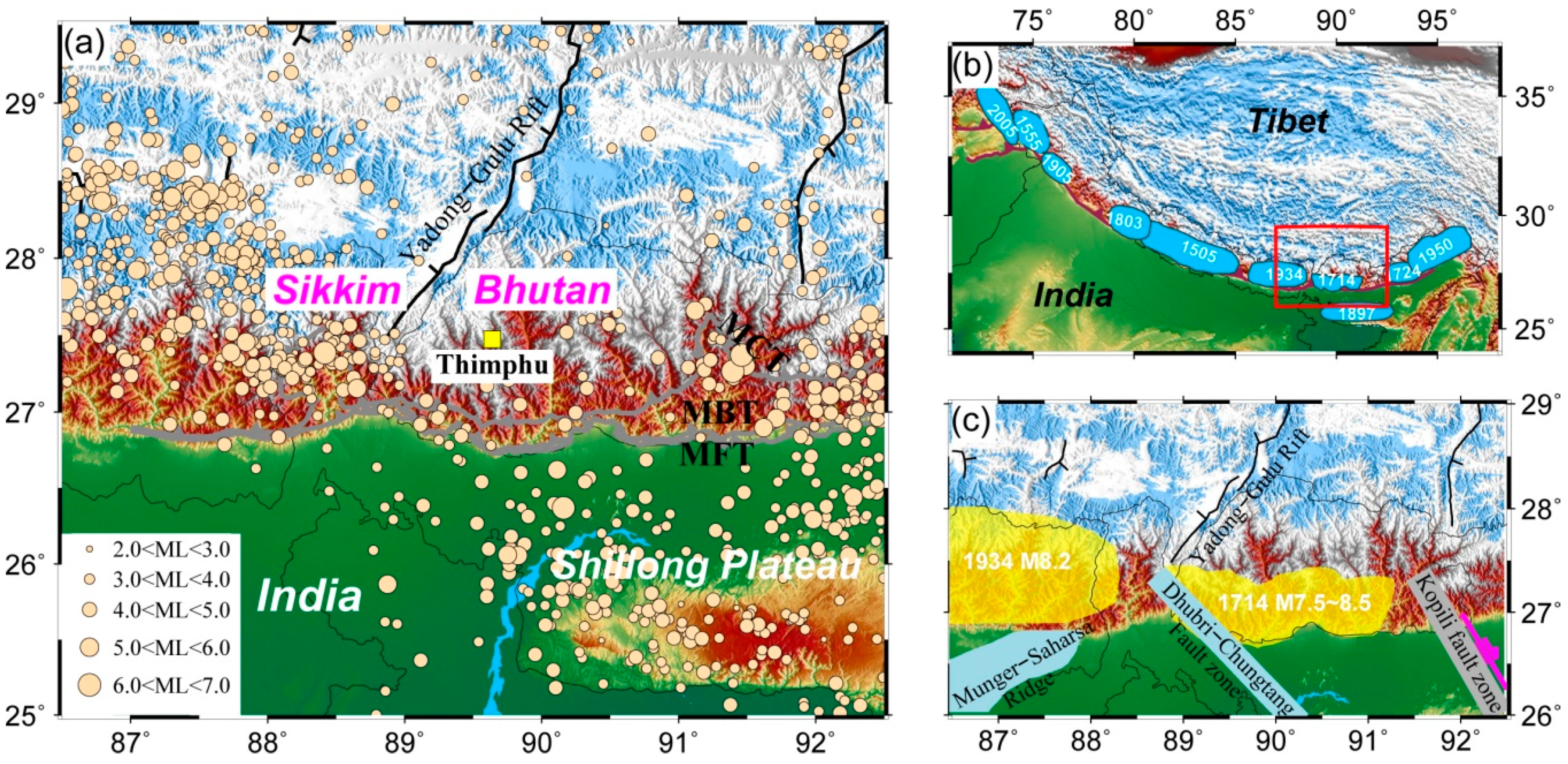
2. Seismotectonic Settings

The present-day tectonic motion of the Sikkim–Bhutan Himalaya is controlled by the convergence between India and Eurasian plates. The convergence deformation is mainly accommodated by the Main Himalayan Thrust (MHT), which represents the basal décollement between the southern Tibet and the rigid India plate. At the surface, the MHT imbricates into three south-vergent thrust faults, i.e., the Main Frontal Thrust (MFT), the Main Boundary Thrust (MBT), and the Main Central Thrust (MCT). The three thrust faults separate the Himalayan ranges into three tectonostratigraphic units, namely the Sub-Himalaya, the Lesser Himalaya, and the Higher Himalaya. The metamorphic grade of the three tectonostratigraphic units increases gradually from south to north, reflecting the progressive migration of the front of the Himalaya to the South through time [26]. The northernmost Higher Himalaya is mainly composed of high-grade metamorphic rocks, with plentiful proofs for partial melting. The Lesser Himalaya is overthrusted by the South margin of the Higher Himalaya along the MCT. In the South of the MCT, the Lesser Himalaya in the Bhutan Himalaya is characterized by a complex duplex structure, associated with many internal thrusts. This duplex structure suggests a southward propagating sequence that initiated after the cessation of tectonic activity on the MCT [27]. In the Sikkim–Bhutan Himalaya, the width of the Lesser Himalaya shows obvious lateral variations along-strike. The width of the Lesser Himalaya increases significantly from western Bhutan to the East. The southernmost tectonostratigraphic unit is the Sub-Himalaya or Siwalik thrust belt. The Siwaliks in Bhutan consist of a narrow and single discontinuous thrust sheet, in contrast with the wide and structurally complex zone in the western Himalaya.
Different from other segments of the Himalayan orogenic belt, the complexity of the regional deformational pattern in the Sikkim–Bhutan Himalaya is obviously added due to the existence of the Shillong Plateau in the foreland (Figure 1c). The clockwise rotation of the Shillong Plateau relative to the rigid India plate greatly influenced the convergence rate and strain partitioning in the Sikkim–Bhutan Himalaya [28]. Previous studies suggest that the uplift of the Shillong Plateau accommodated the convergence rate of ~6 mm/y across the plateau, which nearly represents one third of the total convergence rate of 18 mm/y across the boundary zone [29]. However, this was not supported by recent GPS measurements in the Sikkim–Bhutan Himalaya [28,30]. The GPS-derived shortening rate of 14~21 mm/y across the eastern Himalayas seems consistent with the contraction rate in the central Himalaya [31]. Additionally, recorded seismicity and moment tensors reveal the existence of a dextral Dhubri–Chungtang fault zone at the northwestern margin of the Shillong Plateau that connects the deformation of the Shillong Plateau and the Sikkim Himalaya (Figure 1c) [32,33].

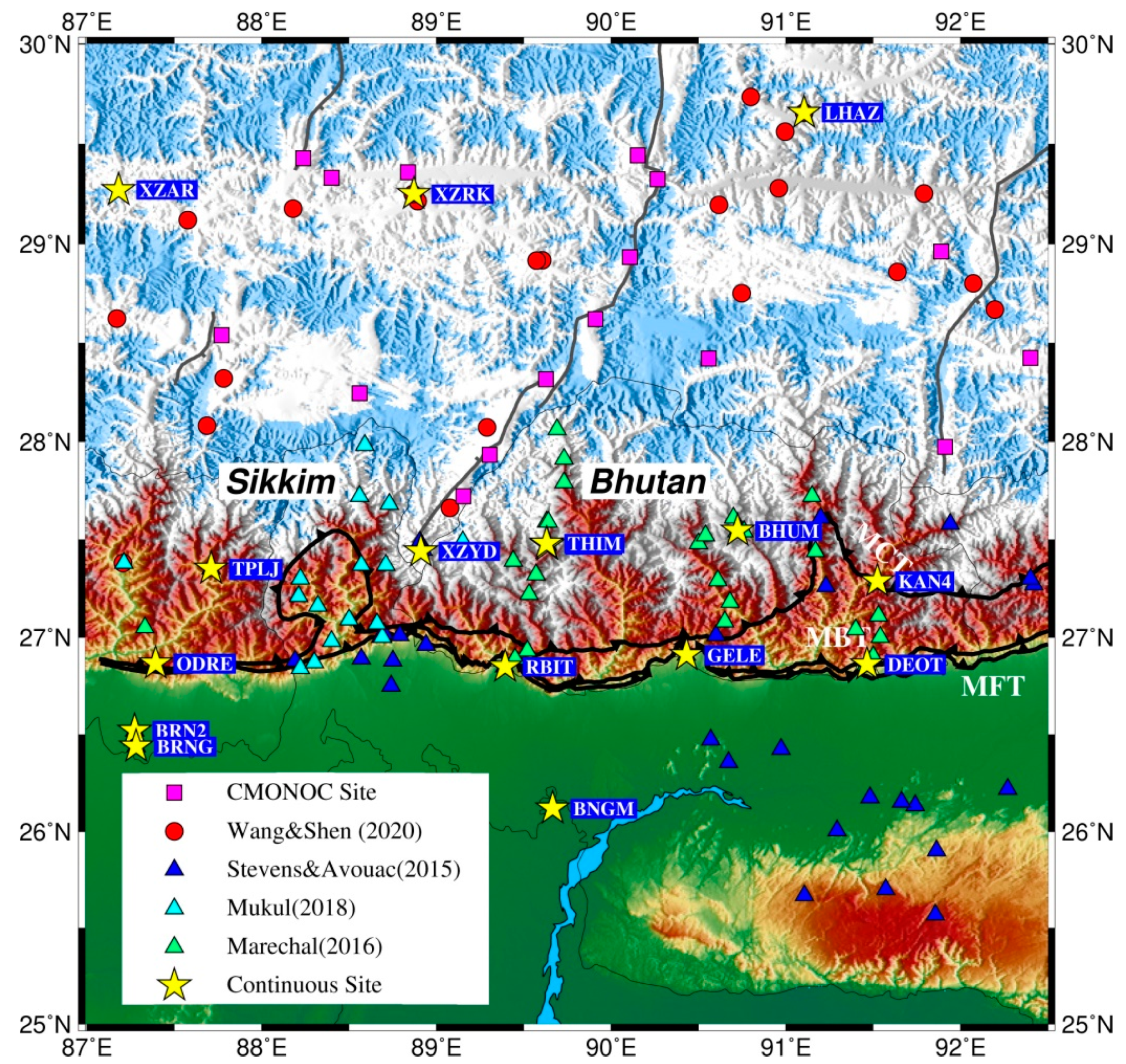
3. GPS Measurements and Velocity Estimation

3.1. GPS Data Processing

In the frontal part of the Sikkim–Bhutan Himalaya, Stevens and Avouac [21] have compiled the majority of the available GPS velocities from literatures that were published before 2015 [34,35]. Additionally, many extended GPS networks have been constructed in the Sikkim–Bhutan Himalaya during the past few years, significantly improving the spatial density of GPS measurements (Figure 2). These extended GPS networks consist of two parts: (1) Nine new stations were installed in the frontal Darjiling–Sikkim Himalaya, with a long time span from 1998 to 2009, to reveal the active deformation pattern in this region [36]; (2) In the central and eastern Bhutan, nine new campaign sites were built and measured from 2013 to 2016. Moreover, four old campaign sites were also reoccupied between 2013 and 2016. In combination with the seven continuous stations in Bhutan (Figure 2), they constitute an unprecedented GPS network in Bhutan to monitor the strain buildup along this segment of the Himalayan arc [6,28]. The velocities of the campaign sites relative to various reference frames are translated into a uniform Eurasia-fixed reference frame through rigid body rotation, which minimizes post-fit residuals at the common stations in different datasets. The position time series of continuous sites in the Sikkim–Bhutan Himalaya are acquired from the University Navstar Consortium (UNAVCO) website (ftp://data-out.unavco.org/pub/products/position).
To the north of the Sikkim–Bhutan, the CMONOC project has installed about 20 stations in southern Tibet since 1999. These stations have been measured at least five times [37]. Besides, about 20 campaign GPS stations around the northern border of Sikkim and the kingdom of Bhutan have also been constructed during the past years. These sites are mainly placed on rock outcrops where possible but, in some cases, on large boulders. More than three periods of observation for each campaign site are conducted. Each site is observed for at least 36 h in each campaign. These data provide additional constraints on the motion of the MHT beneath the Higher Himalaya. The CMONOC data are processed using the GIPSY-OASIS-II software [38]. Full details of the processing are available in Li et al. [39]. The campaign GPS data were processed by Wang and Shen [40] using the GAMIT/GLOBK software. The postseismic effects of mainly large earthquakes were considered in the position time series to obtain a more robust estimation of long-term velocities.

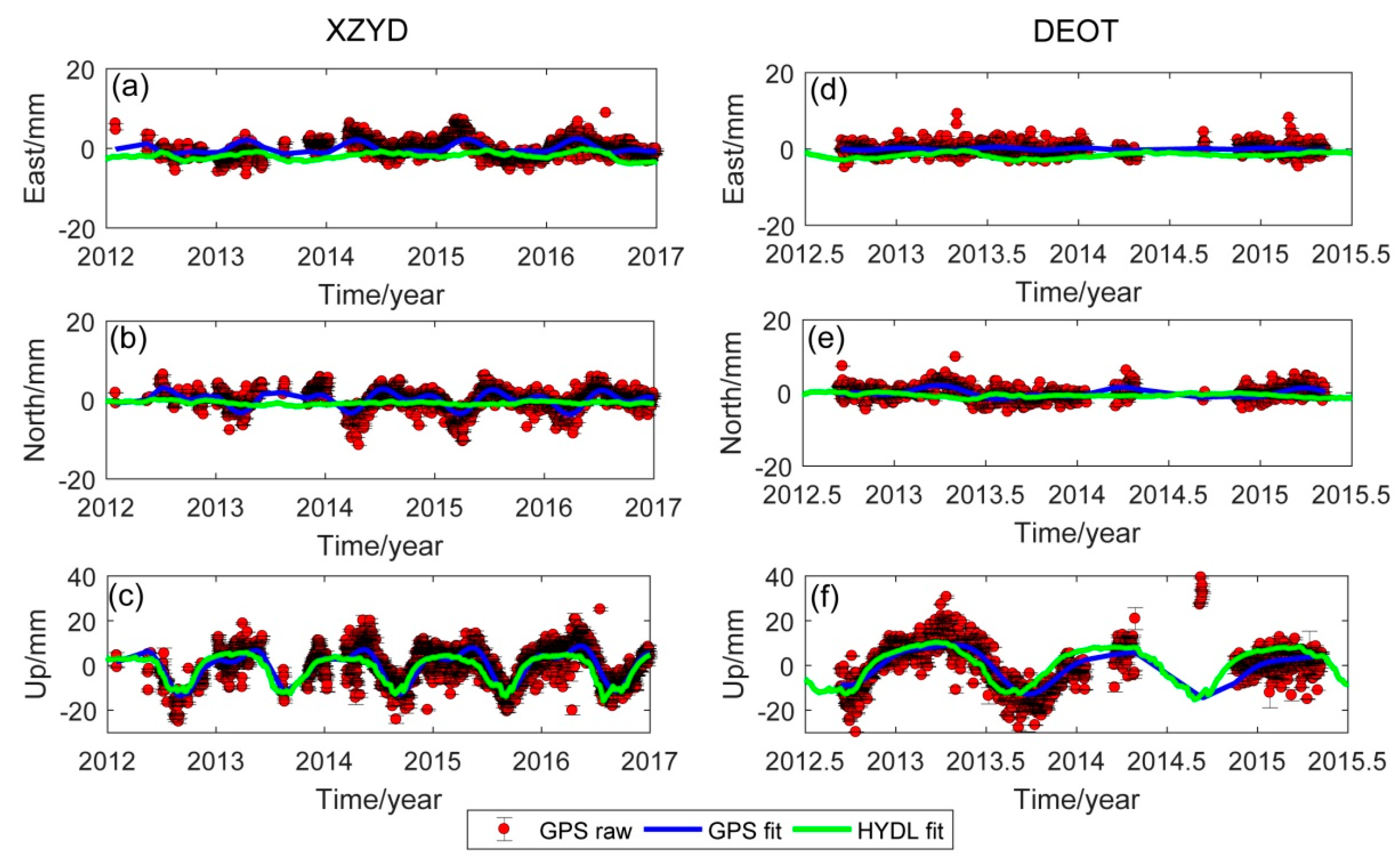
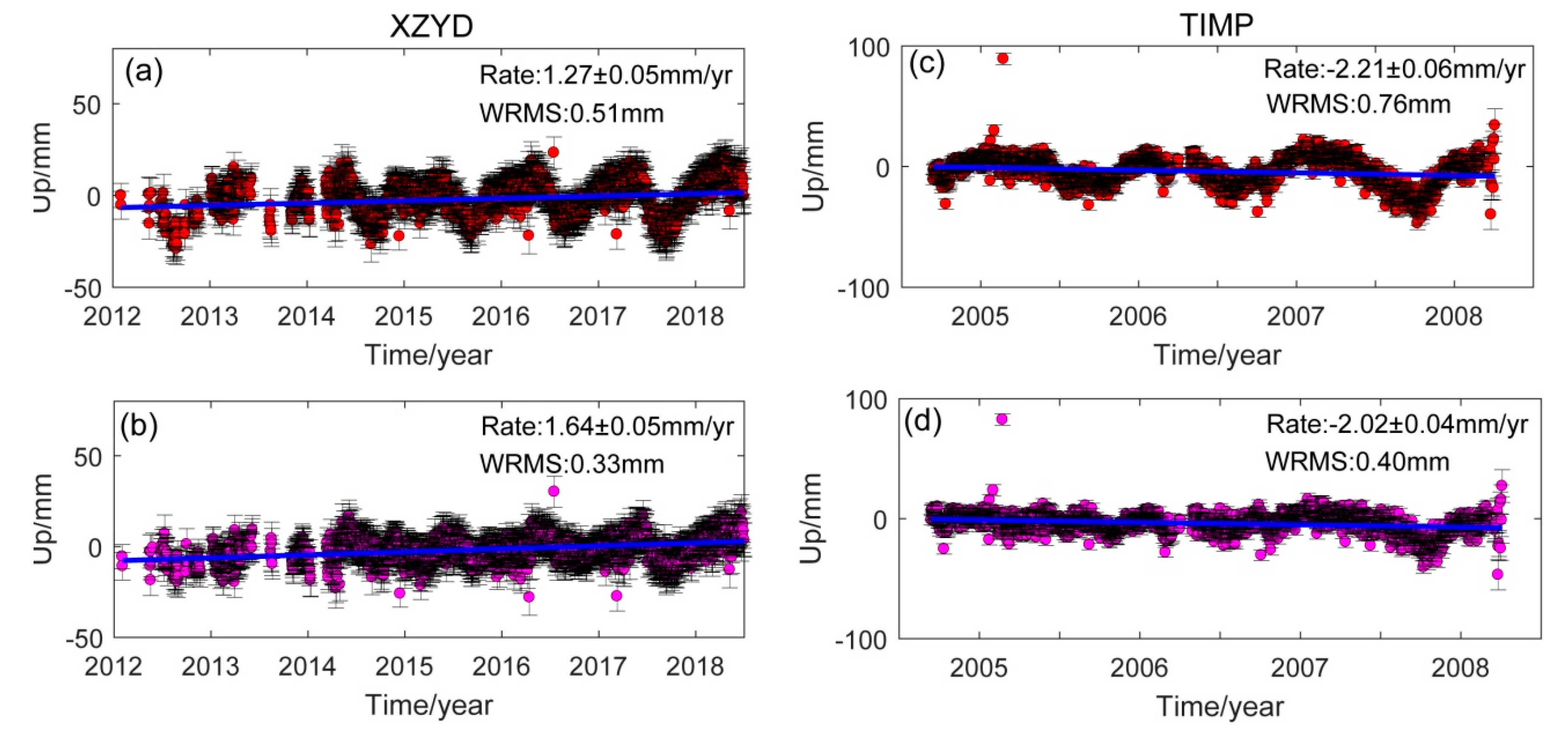
3.2. Correction Due to Hydrological loading Deformation

The seasonal variation in the GPS time series caused by the rainfall in the summer is an important non-tectonic signal that could bias the estimation of interseismic velocity [41]. To accurately determine the three-dimensional velocity field of the Sikkim–Bhutan Himalaya, we need to remove the seasonal effects from the site position time series. In this paper, we use the surface deformation time series at each site due to the Hydrological Mass Loading (HYDL) provided by the GeoForschungsZentrum (GFZ) loading service (https://www.gfz-potsdam.de/en/esmdata/loading), to evaluate and correct the influence of the hydrological cycle. In the HYDL model, elastic surface deformations due to hydrological loading are calculated using a patched Green’s function method, in which the “ak135” elastic earth model is adopted to estimate the load Love numbers [42]. The daily solutions of surface displacement are given on a regular global grid with a size of 0.5° × 0.5°. More details about the calculation could be found in Dill and Dobslaw [42].
In Figure 3, we compare observed GPS time series with the HYDL-predicted displacements for two typical sites (XZYD, DEOT). We can see strong correspondence between the GPS-observed and HYDL-predicted seasonal variations in both the amplitudes and phases for the vertical components, while the correspondence between the GPS-observed and HYDL-derived seasonal variations for the East and North components is less well. We think this difference could be influenced by a small horizontal signal and the spatial smoothing of the HYDL model. Therefore, we only use HYDL predictions to correct the hydrological influences from the vertical components of the detrended GPS time series of each continuous site. We do not correct the hydrological effects of campaign sites due to their limited observation time periods. Generally, the misfit between data and linear fit decrease significantly after the correction. We choose the continuous GPS stations XZYD and TIMP for examples. Figure 4 shows the comparison of the vertical GPS time series before and after correcting hydrological loading effects. The Weighted Root Mean Square (WRMS) is after the correction decreased by 35% (from 0.51 mm to 0.33 mm) and 47% (from 0.76 mm to 0.40 mm) for sites XZYD and TIMP, respectively. We note that some residual seasonal variations still can be recognized in the corrected time series after removing seasonal effects using the HYDL mode (Figure 4b). This indicates that the seasonal variations in the GPS-observed time series are not only caused by hydrological mass loading effects. Many other factors, such as the atmosphere mass loading, could also contribute to generating the seasonal variations in the GPS time series. After correcting the hydrologic loading effects, we re-estimate the vertical velocities for the 15 continuous sites. The estimated velocities with respect to the International Terrestrial Reference Frame 2008 (ITRF08) inference frame are then transformed into the Eurasia-fixed frame using the Euler vector presented by Altamimi et al. [43]. The uncertainties of the GPS horizontal and vertical velocities for most sites are less than 1.0 and 1.5 mm/y, respectively. The derived horizontal and vertical velocity field in the Sikkim–Bhutan Himalaya is shown in Figure 5.

4. Modeling of Interseismic Coupling in the Sikkim–Bhutan Himalaya

4.1. Slip Rate on the MHT

Refining the coupling distribution on the MHT requires precise characterization of the long-term convergence rate. Here we adopt the GPS-derived slip rates on the MHT to represent the long-term convergence rate. We assume that the plate convergence rate is accommodated through stick-slip on the shallow part of the MHT, while the deep portion of the MHT creeps freely. Thus, the concept of the deep slip model can be used to estimate the convergence rate [44]. We project arc-normal velocity components onto three 120-km-wide velocity cross sections in the Sikkim–Bhutan Himalaya (Figure 5). The arc-parallel components of velocity are neglected because this motion is likely to be caused by independent structures within the overriding plate, rather than the stick-slip on the MHT [36]. A grid search method is performed to estimate the best-fitted fault parameters (fault dip, locking depth and the slip rate) (Figure 6).

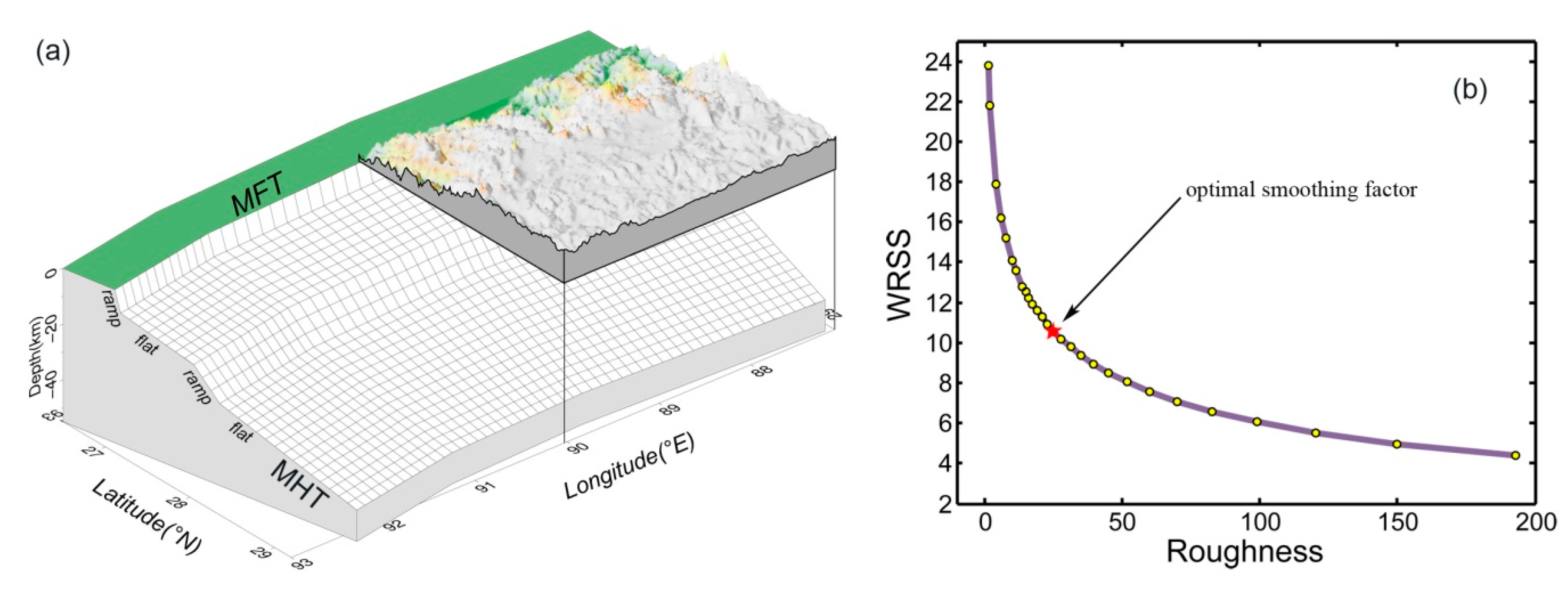
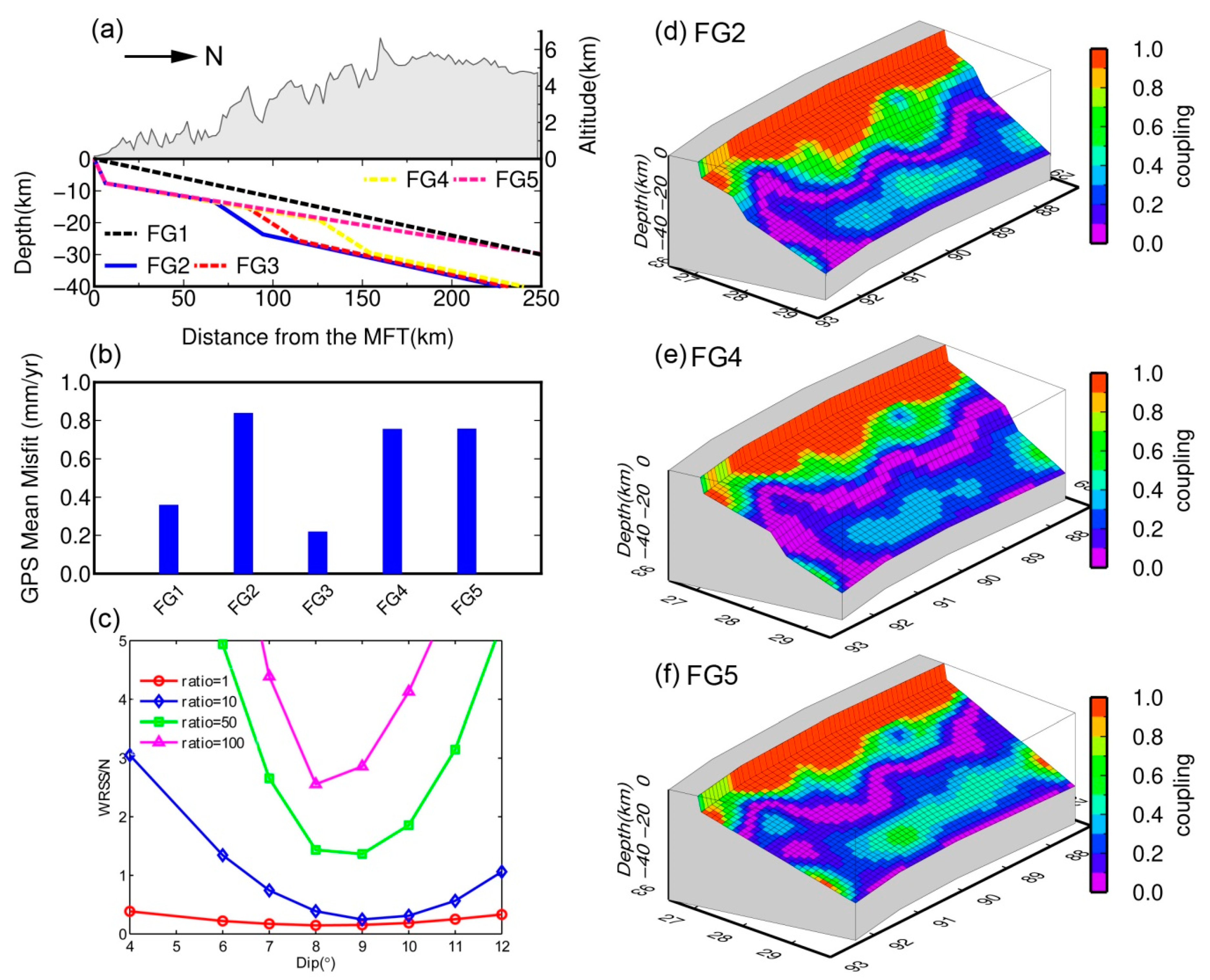
4.2. Fault Geometry of the MHT

The realistic fault geometry of the MHT in the Sikkim–Bhutan Himalaya is still debated. Robert et al. [27] suggested that the MHT in Bhutan is characterized by a continuous shallowly dipping detachment without a ramp below the Higher Himalaya according to inversion of the Apatite Fission Track (AFT) age data, while several studies suggest that the geometry of the MHT is actually more complex. In the Sikkim segment, Acton et al. [45] recognized a ramp-like structure in the receiver function image, similar to the geological postulated position of the MHT in Nepal [46]. The INDEPTH profile along the Yadong–Gulu rift in southern Tibet also clearly reveals the ramp on the MHT that dips northward at 15°–20° beneath the northern Tethyan belt [47]. In western Bhutan, the geometry of the MHT is identified by Singer et al. [48] using the receiver function imaging method. The sub-horizontal flat portion of the MHT is located at the depth of ~14 km with an average width of 80~100 km. In the North, a steep mid-crustal ramp beneath the Higher Himalaya with a dip of ~18° is connected to this sub-horizontal flat. However, through the joint inversion of GPS measurements, Holocene uplift rates and denudation rates at the frontal Himalaya, Roux–Mallouf et al. [49] inferred that the mid-crustal ramp structure in western Bhutan is actually connected to a 130-km-wide flat portion of the MHT. This suggests that the upper flat of the MHT in western Bhutan is much wider than the shallow flat in Sikkim and central Nepal. The discrepancy between geological results and geophysical images could be attributed to the differences in the considered timescales. Additionally, previous studies also suggest that the fault structure in the Bhutan Himalaya may vary along-strike [50,51]. The width of the upper flat of the MHT in eastern Bhutan is slightly narrower than in western Bhutan [48,50].
In this study, we construct the fault geometry of the MHT in the Sikkim–Bhutan Himalaya in combination with all the thermochronological ages, seismic reflection and receiver function profiles. Although the strict structure of the MHT beneath the Sikkim–Bhutan Himalaya remains controversial, we can describe the first-order geometry of the MHT as a double-ramp structure (Figure 7a). The double-ramp structure of the MHT consists, from south to north, of four segments. First, a steep frontal ramp (dip = 50°) between the depth of 0–10 km. This segment is constrained by the thermochronological ages [50]; Second, a sub-horizontal flat structure (dip = 6°) between the depth of 10–15 km; Third, a steep mid-crustal ramp (dip = 20°) between the depth of 15–25 km. We assume that the mid-crustal ramp extends from the frontal of the Higher Himalaya to the North; Finally, a sub-horizontal décollement (dip = 7°) beneath the Higher Himalaya and southern Tibet [33,52]. Compared with the simple flat fault structure adopted by previous coupling models [21,25], our fault structure is more complex and realistic, although we neglect the lateral variation of the fault geometry that may exist in fact for ease of modeling. A discussion about the effect of the fault geometry on the coupling model is made in Section 6.1.

4.3. Inversion Strategy

The interseismic crustal deformation in the Sikkim–Bhutan Himalaya is assumed to result from the joint effects of steady block motion, the nonrecoverable intrablock strain and the locking of the block boundary faults [53]. In this study, we first translate the Eurasia-fixed GPS velocity field into the Indian plate reference frame to remove the steady block motion components of southern Tibet, relative to the India block. In addition, GPS measurements in the Shillong Plateau revealed that the Shillong block is rotating clockwise, relative to India [28]. We adopted the rotation pole for the Shillong with respect to the India block estimated by Vernant et al. [28] (longitude = 88.78°E, latitude = 26.43°E, rotation = -1.149°/Ma) to remove the rotation components from GPS velocities in Bhutan. Except for the elastic responses due to strain accumulation on the MHT, the GPS velocities in southern Tibet also include the deformation from regional South–North trending grabens, such as the Yadong–Gulu rift. We use a priori geological deformation model given by Armijo et al. [54] which assumes homogeneous extension rates for rift zones, to remove the extension components from the GPS velocity at each site. The remaining GPS velocities in the Sikkim–Bhutan Himalaya, which only reflect the elastic motion of the hanging wall (southern Tibet block) relative to footing walls (India and Assam blocks), are then used to invert the interseismic coupling distribution.
We calculate the coupling coefficient through inverting the distribution of slip deficit on the MHT. The back-slip dislocation approach proposed by Savage [44] has been widely used to invert for the slip deficit on subduction zones [12,13,14,15,16]. However, it should be noted that the back-slip model can only be used for planar structures of faults. When considering the complicated fault geometry, like the double-ramp structure of the MHT, the back-slip model will lead to deformation anomalies that cannot be neglected, especially at the place where fault emerges [55]. In this study, the slip deficient components (dip-slip and strike-slip) are inverted directly on the MHT, similar to the inversion of the co-seismic slip [56].This approach has been used in the modeling of coupling in the central Nepal Himalaya and the Altyn Tagh fault [22,57]. We define the ratio between the fault slip deficit rate and the GPS-derived long-term convergence rate as the coupling coefficient. The slip rate of each segment is allowed up to the corresponding convergence rate, so the coupling coefficient can be described using a value between 0 and 1. When coupling = 1, the subfault is completely locked, and when coupling = 0, the subfault is fully creeping. The coupling coefficient between 0 and 1 means that the subfault is partly locked.
The interface of the MHT is discretized into 51 × 27 subfaults with an average size of ~10 × 10 km (Figure 7a). The Green’s function that links the slip at each subfault and surface displacement is calculated using rectangle dislocation in a homogeneous elastic half-space [58]. The smoothing factor that can detect the coupling variation along-strike is determined according to the trade-off curve between the slip roughness and the Weighted Residual Sum of Squares (WRSS) (Figure 7b). The relative weight between the GPS horizontal and vertical displacement components for continuous GPS sites are determined by their formal errors. We estimate the slip on each path using the non-negative least square algorithm [59], which minimizes misfits to surface displacements subject to weighted constraints on the roughness of the slip distribution. We only use the dip-slip components to calculate the coupling coefficient, despite the fact that both strike-slip and dip-slip components are estimated during the inversion. We find that the estimated strike-slip components are very small for most patches (<3 mm/y). The strike-slip components could reflect the motion of many local strike-slip faults rather than the slip on the MHT [36].

5. Results

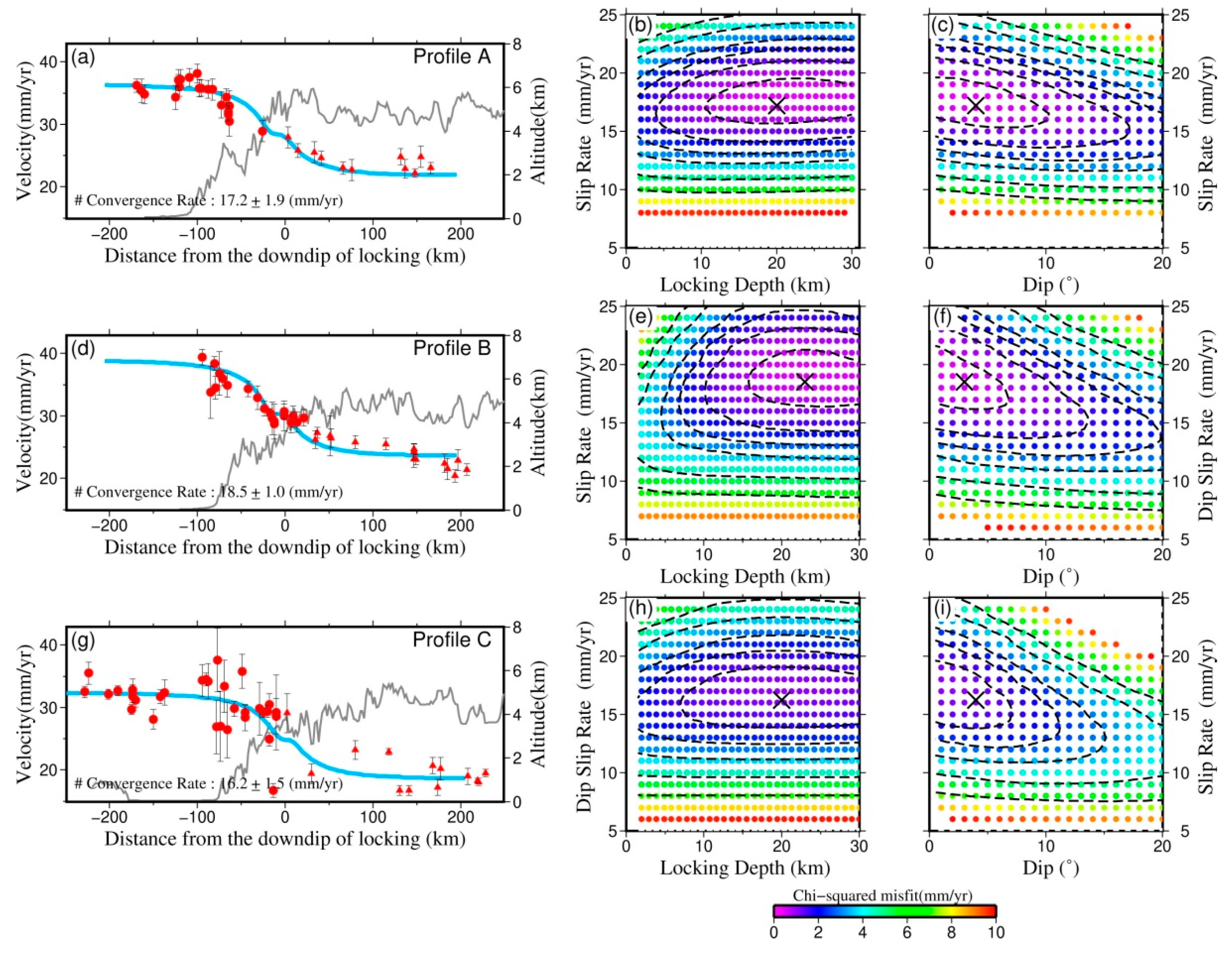
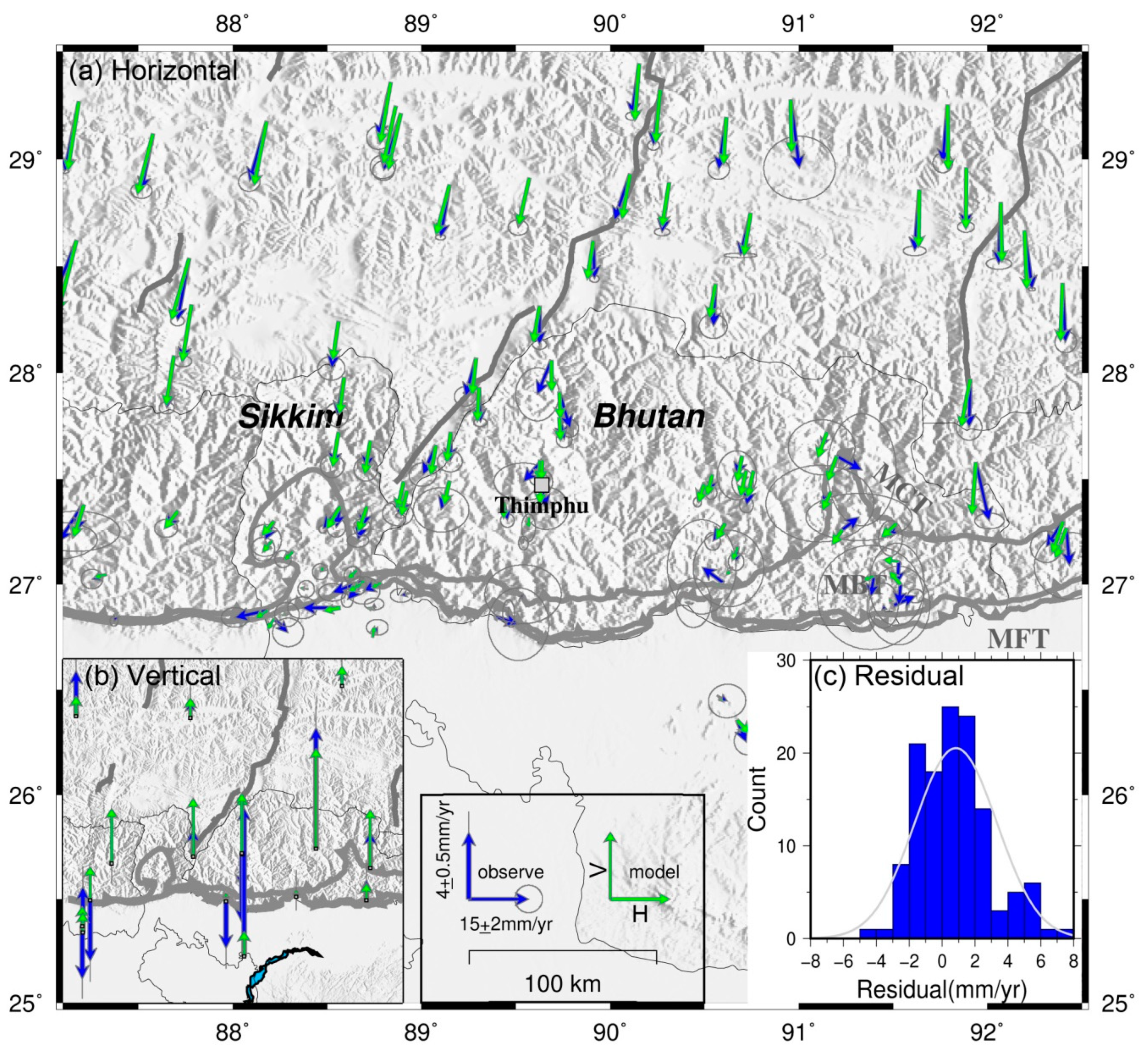
5.1. Convergence Rates across the Sikkim–Bhutan Himalaya

Figure 6 shows the grid search result for the three cross sections using χ2 method with varying fault parameters. Generally, the grid search method reveals relatively significant trade-off effects between the slip rate, locking depth and fault dip. The results provide very good constraints on the convergence rate across the Sikkim–Bhutan Himalaya, while the locking depth and the fault dip are not very tightly constrained which could attribute to the large uncertainty of the velocities at some campaign sites. Here, we mainly analyze the characteristics of the convergence rates regardless of the fault dip and locking depth. The characteristic of fault locking is analyzed in Section 5.2.
In the Sikkim Himalaya (Profile A), a convergence rate of 17.2 ± 1.9 mm/y is estimated by GPS measurements, and it generally coincides with the estimated slip rate of ~18 mm/y measured by Mukul et al. [36]. Most of the convergence deformation is absorbed in the south of the South Tibet Detachment (STD), in which, nearly about half of the active convergence is confined to the Lesser Himalaya [36]. In the west of Sikkim, the 1934 Mw 8.2 earthquake ruptured a zone of at least 150 km along the trace of the MFT [60]. The GPS-measured interseismic velocities in this region could be affected by the postseismic viscoelastic deformation of this event. Recent studies suggest that the viscoelastic relaxation due to the 1934 event would enlarge the convergence rate across eastern Nepal by approximately 3 mm/y, but in the Sikkim segment, this effect is no more than 2 mm/y. This implies that the estimated convergence rate here is temporally stable and can represent the long-term convergence deformation [39,61].
In western Bhutan (Profile B), we estimate a convergence rate of 18.5 ± 1.0 mm/y, slightly larger than the convergence rate of 14~16 mm/y simulated by Vernant et al. [28]. The difference might attribute to more GPS data in southern Tibet being used in our estimation which provides tighter constraints on the upper bound of the estimated convergence rate. In eastern Bhutan (Profile C), the estimated convergence rate is 16.2 ± 1.5 mm/y, general in agreement with that in western Bhutan. Burgess et al. [62] estimated a convergence rate of 23 ± 6.2 mm/y across eastern Bhutan according to the age and geometry of uplifted river terraces. Their estimated convergence rate is quite larger than that which we derive from GPS measurements, although their estimation shows a large uncertainty. The significant discrepancy between the long-term slip rate from geological study and our geodetic estimate suggests that some parts of the interseismic deformation in eastern Bhutan could be anelastic.

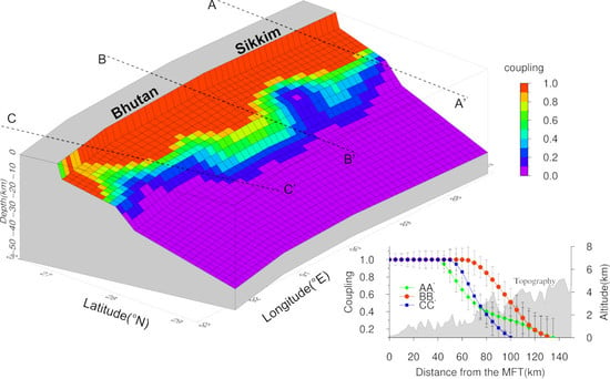
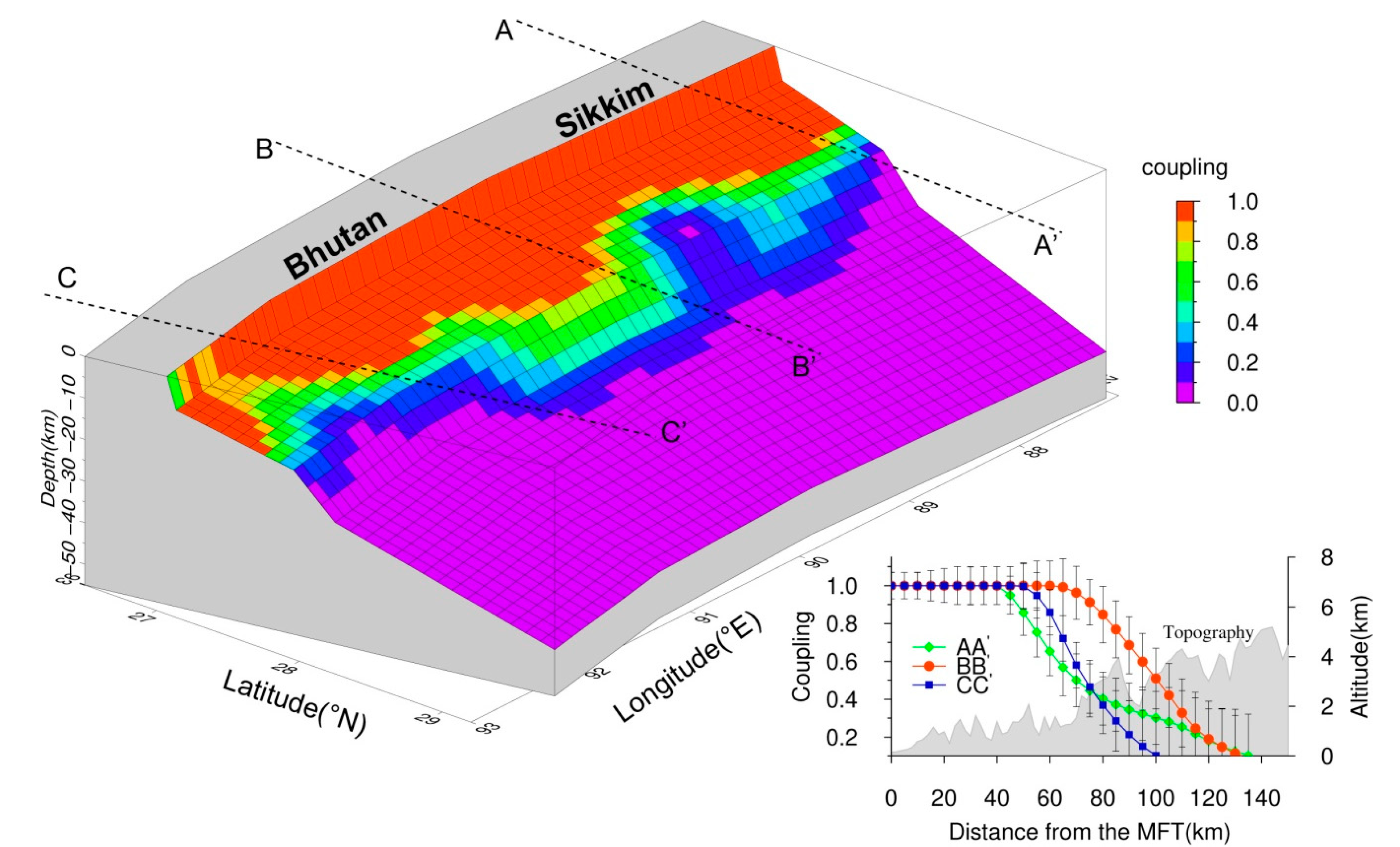
5.2. Interseismic Coupling along the MHT

The preferred interseismic coupling model is shown in Figure 8. The fitness to the GPS observations is shown in Figure 9. The modeled surface velocities are comparable with the observations with mean misfits of 0.8 and 1.2 mm/y for the GPS horizontal and vertical velocities, respectively. Generally, the MHT beneath the Sub and Lesser Himalaya is strongly coupled without showing any obvious creeping zones, similar to the Nepal and Kashmir segments [20,21]. While some lateral variations for coupling still can be recognized. The most obvious characteristic is that the locking width in western Bhutan is much wider than in Sikkim and eastern Bhutan. Three coupling transects are projected to reveal the along-strike variations of coupling distributions (Figure 8). The locking width (coupling > 0.5) in the Sikkim segment is 60~70 km, coinciding with the width of the décollement in this region, both of which are anomalously narrow [28]. In western Bhutan, the locking width reaches ~100 km, which is much wider than the locking width of ~70 km in eastern Bhutan. At the eastern border of Bhutan, a less strongly coupled region at shallow depth can be recognized, although the retrieval ability of geodetic data here is relatively weak (see Figure 10). The 1714 M 7.5~8.5 earthquake occurred on the shallow part of the MHT in western and central Bhutan [8]. The rupture zone of this event, which has been constrained effectively using historical intensity data and empirical scaling law, reaches to the surface trace of the MFT. The rupture zone of this event is mainly confined to the strongly coupled patches. Along the downdip of the rupture zone, both locking and creeping on the MHT can be observed, suggesting a large strain gradient in this region.
The inversion results indicate that the shallow ramp between the depth of 0~10 km is almost full coupling for most of the Sikkim–Bhutan Himalaya, while the coupling pattern on the mid-crust ramp shows obvious along-strike variations. The mid-crust ramp in Sikkim and eastern Bhutan is nearly free creeping with a small coupling coefficient (coupling < 0.3). In western Bhutan, the mid-crust ramp is partly coupled (0.3 < coupling < 0.9). Following Bilham et al. [63], we define the partly coupled area as the interseismic decoupling zone. As shown in Figure 8, a continuous interseismic decoupling zone with a width of 40~60 km along the Sikkim–Bhutan Himalaya can be recognized, which is significantly shorter than the typical width of interseismic decoupling zones in subduction zones [64]. Most of the historical earthquake in the Himalaya nucleated in the interseismic decoupling zone [11]. It is noteworthy that there is an embayment of decoupling zone near the border between Sikkim and western Bhutan, similar to the western Nepal Himalaya (~83°E) [21,65]. From 88°E to 88.7°E, a rapid decrease in the locking width on the MHT can be recognized, and then from 88.7°E to 89.5°E, we can see a rapid increase in the locking width, showing an embayment-shaped zone of fault locking. We suggest that the embayment of decoupling zone is a robust feature because the coupling distribution in the embayment zone can be resolved in a high spatial resolution thanks to the dense geodetic data in this region.

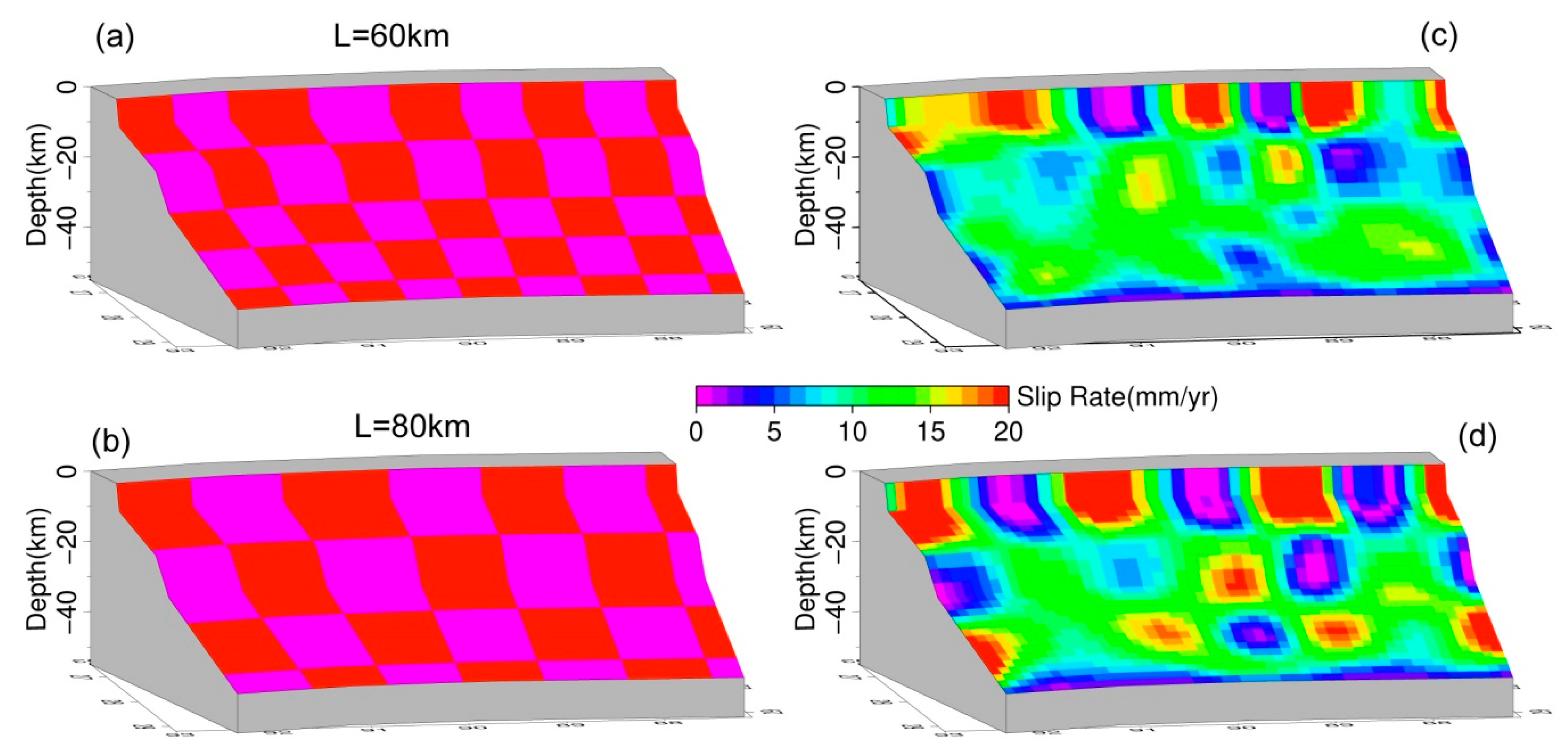
5.3. Resolution Test

We perform a series of checkerboard tests to assess the average spatial sizes of coupling that can be resolved using the GPS observations on the given fault geometry. We test two different input asperity models. In the two models, the widths of the input fault checkerboard are set as 60 km and 80 km, respectively. The surface displacement at each GPS station is calculated according to the input checkerboard model. We then add some random Gaussian noises into the synthetic displacements to represent the uncertainties of the input data. The mean and standard deviations of the random Gaussian noises are determined based on the real GPS velocities. The synthetic inversion results are shown in Figure 10. It can be seen that the input slip patches above the depth of 40 km can be well resolved if the size of the input checkerboard is larger than 80 km, although the recovering ability decreases with depth. When the dimension of the input checkerboard is smaller than 60 km, the coupling patches at shallow depths (0~25km) still can be retrieved satisfactorily— except for northeastern Bhutan where the GPS distribution is relative sparse. Based on the results of the checkerboard test, we conclude that the main characteristics of the interseismic fault locking in the Sikkim–Bhutan Himalaya can be well resolved by the 3D GPS measurements.

6. Discussion

6.1. Effect of Fault Geometry on the Coupling Model

The adopted geometry of the MHT is necessarily a simplification of the complex fault systems in the Sikkim–Bhutan Himalaya based on previous studies. The uncertainty of a prior geometrical model of the MHT may affect the results of the fault coupling. To an extent, any variation in the fault geometry that can significantly disturb our coupling estimation is our concern, for which we test a series of geometrical models of the MHT, including the planar flat model (FG1), the double-ramp model with varying widths of upper-crust flat (FG2–FG4) and the single-ramp model (FG5) (Figure 11a). We assume that all the interface configurations intersect the surface along the MFT. All available GPS observations are included to constrain the coupling pattern on the assumed fault interface. The model misfits are shown in Figure 11b, and the inverted coupling distribution based on fault models FG2, FG4 and FG5 are shown in Figure 11d~f, respectively.
It can be seen that the double-ramp model with the width of upper-crust flat of approximately 80 km (FG3) can explain the surface observations slightly better (Figure 11b). Too narrow (FG2) or too wide (FG4) for the upper-crust flat in the geometrical models results in larger data misfits, although the main features of inverted coupling distribution are largely unchanged. Compared to the double-ramp structure, the single-ramp model (FG5) cannot explain the observations better. Although the planar flat model (FG1) can fit the surface observations slightly better than the single-ramp model, its interface configuration is a little far from the realistic fault geometry of the MHT based on geophysical and geological studies. In general, the first-order characteristics of the coupling distribution can be well resolved through different geometrical models, suggesting that the interseismic coupling distribution could be not very sensitive to fault geometry. In other words, the interseismic data in this study are not sufficient to precisely constrain the fault geometry of the MHT, which is coherent with previous studies, for example, Grandin et al. [66] also found that the inversion of GPS data provides no constraint on the fault dip of the MHT. Instead, it can provide good constraints on the slip rate and locking depth.
One main factor resulting in the insensitivity of fault geometry to interseismic data is that the interseismic signal is usually with a relatively weak Signal-to-Noise Ratio (SNR) and easily contaminated by some local effects, such as ice melting and human activities. In order to assess the influence of the uncertainty of GPS velocities to the sensitivity of fault geometry, a number of experiments are conducted. We mainly focus here to explore the correlation between fault dip and coupling distribution. The effect of other fault geometry parameters, such as length, width and strike, can be ignored [67]. The single-ramp model (FG5) is adopted in the test. We regard the fitted 3D GPS velocity field in Figure 9 as the input data setting different uncertainties. The model residuals clearly show that the sensitivity of the fault dip strengthens markedly with the increase in the SNR for GPS velocities (shown in Figure 11c). When the SNR can be improved by a factor of 10, the fault dip could be uniquely determined by the GPS velocities. This could explain that the GPS velocity field with a longer period can interpret the interseismic deformation better for its improved SNR.

6.2. Connections between Interseismic Coupling, Fault Geometry and Seismic Activity

The spatial variation of coupling distribution is an essential factor that needs to be considered when we interpret relationships with the seismic activity. Here we compile all available earthquake catalogs in the Sikkim–Bhutan Himalaya to analyze the spatial relationships between the geometry of the MHT, the interseismic coupling, and the seismicity (Figure 12). The record of earthquakes used in the analysis consists of three parts: (1) Seismicity from the International Seismological Centre–Global Earthquake Model (ISC-GEM) Catalog (1900-1973) [68]; (2) The National Earthquake Information Center (NEIC) bulletin (1973–2015); (3) Earthquake catalog with time span of 2012–2014 supplemented by the Geodynamics ANd Seismic Structure of the Eastern Himalaya Region (GANSSER) network [33]. In the Sikkim Himalaya (Figure 12b), the belt of seismicity is mainly contained in the interseismic decoupling zone, although these events are not mainly focused on the interface of the MHT. Focal mechanisms of moderate-sized earthquakes in the Sikkim region suggest that the Sikkim Himalaya is characterized by a strike-slip motion on a transverse tectonic, which is different from the typical thrust tectonics in the Himalayan subduction zone [69]. This perhaps can partially explain the diffused seismicity in depth in the Sikkim Himalaya. In the Bhutan Himalaya (Figure 12a), the narrow band of seismicity appears to disappear. The seismicity in Bhutan is broadly distributed, implying that the interseismic strain accumulation beneath Bhutan could be broadly distributed rather than only in the front of the Higher Himalaya. This is supported by the normalized river-channel steepness (Ksn) in the Himalaya that is interpreted to be indicators of the rock uplift rate over a time scale of 104–105 years [70] (Figure 12e). The high-Ksn rivers in Bhutan are clustered into two bands, significantly different from the single cluster of high-Ksn rivers in Nepal that is located north of the band of seismicity.
In western Bhutan (Figure 12c), a cluster of earthquakes beneath the Higher Himalaya displays a strong correlation with the interseismic decoupling zone, consistent with the location of the mid-crust ramp and the 3500 m topographic contour at the surface. Moreover, it is interesting to note that a large number of earthquakes occurred below the MHT with the depth of 20~40 km in western Bhutan, which can be interpreted due to the thickened crust and the strike-slip structure in the Indian basement [32,33]. In contrast, the seismicity in eastern Bhutan mainly concentrates on the interface of the MHT (Figure 12d). The earthquakes in the mid-crust ramp of eastern Bhutan are rarely distributed, which is consistent with the low coupling coefficient in this region. The abundant seismicity in the strongly coupled segment of the MHT in eastern Bhutan, compared with the absence of seismicity in the West, suggests possible differences in current strain accumulation on the MHT between the western and eastern Bhutan Himalaya.
Generally, the seismic activity in the Bhutan Himalaya shows significant differences to other segments of the Himalayan seismic belt, although the convergence rate and the interseismic decoupling zone are similar to the rest of the Himalayan range [27,65]. This implies that the recent seismicity in the Bhutan Himalaya could not be uniquely controlled by the convergence rate and the stress buildup on the interface of the MHT. Other factors, such as the geometry of the subduction structure, crustal thickening and/or the change in rheology could also partly drive the seismicity in the Bhutan Himalaya [9,71]. It should be noted that the GPS-derived coupling map in the Sikkim–Bhutan Himalaya reflects the strain accumulation over only decades of years, which is expected to show some discrepancies with the seismic activity that indicates stress buildup over thousands of years. Additionally, considering the fact that the instrumental record is not sufficiently long, the seismicity record in the Sikkim–Bhutan Himalayan is not representative of the long-term seismic cycle, which might also influence our analysis.

6.3. Implication for Strain Segmentation and Earthquake Hazard

The latest large earthquake that ruptured the Bhutan Himalaya is the 1714 M7.5~8.5 earthquake. No major earthquakes in the past 300 years and strong strain accumulation in the Bhutan Himalaya suggest a seismogenic potential in the near future. Our results reveal an embayment of decoupling zone near the border between Sikkim and western Bhutan, attesting to a narrower coupling region by 30~40 km than the adjacent segments. The embayment of decoupling zone is separated by the rupture terminates of the 1934 M~8.2 earthquake at the west and the 1714 M7.5~8.5 earthquake at the east, respectively [8,60]. It remains unclear which factor controls the rupture of the large historical earthquake along the strike of the Sikkim–Bhutan Himalaya. Previous studies suggested that the Himalayan earthquakes are segmented by prominent ridge interaction or active shear zones [25,33,72]. In the map view, the inverted embayment of decoupling zone lies in the triple junction region of three structures: the Munger–Saharsa Ridge (MSR), the Dhubri–Chungtang Fault Zone (DCF) and the Yadong–Gulu Rift (Figure 1c). It is still difficult to determine which structure dominates the rupture propagation and arrest of large earthquakes in the Sikkim–Bhutan Himalaya. Although other possibilities exist, we suggest that the spatial variation of frictional properties, indicated by the frictional coupling on the MHT, can also explain the segmentation of large Himalayan earthquakes in the Sikkim–Bhutan Himalaya, without the need to consider the geometrical control factors. The eastern border of Bhutan is intersected by the dextral Kopili fault zone in the foreland (Figure 1c), spatial correlates with another narrow coupling zone in this place. If this narrow coupling zone represents another boundary that separates large Himalayan earthquakes, the whole kingdom of Bhutan can be regarded as a relatively complete area that could be ruptured in a future large earthquake.
It is commonly accepted that large Himalayan earthquakes were mainly restricted to the shallow portion of the MHT with high coupling coefficients [11,21]. However, it remains unclear whether the rupture of large earthquakes can propagate into the weakly coupled regions along the downdip of the MHT. In subduction zones, many studies have demonstrated that large megathrust earthquakes can rupture the regions inferred to be less strongly coupled (coupling < 0.3) along the downdip direction [14,16]. In theory, different rupture extensions along the downdip direction of the interface of subduction could result in different magnitudes of earthquakes. If all of the strong coupling regions (coupling > 0.9) in the Bhutan Himalaya are ruptured, an Mw ~8.2 earthquake could be generated considering a steady slip deficit rate of ~17 mm/y since the 1713 earthquake. Meanwhile, if the next large earthquake beneath the Bhutan Himalaya ruptures the MHT downdip to the less strong coupling zones (coupling = 0.3), it could induce an Mw ~8.5 earthquake or even be larger. In any case, it can be concluded that the near-term seismic risk in the Bhutan Himalaya remains very high and deserves special attention.

7. Conclusions

In this study, we estimate a new 3D interseismic GPS velocity field in the Sikkim–Bhutan Himalaya to image the interseismic coupling on the MHT. Our improved measurements yield convergence rates of 16.2~18.5 mm/y in the Sikkim–Bhutan Himalaya, comparable to the convergence rates in the central and western Himalaya. This confirms that the Sikkim–Bhutan Himalaya is not immune from large earthquakes and the Shillong Plateau in the foreland contributes little in accommodating the convergence deformation across the Sikkim–Bhutan Himalaya. The refined coupling model based on a double-ramp structure suggests that interseismic coupling distribution is essentially continuous throughout the MHT. The downdip width of fault coupling in western Bhutan reaches ~100 km, which is 30~40% larger than the coupling widths of Sikkim and eastern Bhutan. This suggests significant along-strike variations of interseismic coupling in the Sikkim–Bhutan Himalaya, which might control the segmentation of great megathrust earthquakes in this region. A continuous interseismic decoupling zone with a width of 40~60 km is recognized in the Bhutan Himalaya, similar to the central Nepal segment. However, the seismic activity in Bhutan is diffusely distributed, rather than being restricted in the interseismic decoupling zone. This implies that the seismic activity in the Bhutan Himalaya is not uniquely controlled by the stress buildup at the downdip end of the locked portion of the MHT.

Author Contributions

T.T. designed the research. S.L. processed the data, performed the result analysis and wrote the original manuscript. Q.W. proposed the thoughtful comments and suggestions of the original manuscript. F.G., X.Q., Y.Z. and J.H. reviewed the manuscript. All authors have read and agreed to the published version of the manuscript.

Funding

This research was funded by National Natural Science Foundation of China: 41731071. Fundamental Research Funds for the Central Universities: JZ2020HGQA0140. Open foundation of State Key Laboratory of Geodesy and Earth’s Dynamics: SKLGED2020-4-2-E.

Acknowledgments

We express special thanks to the Crustal Movement Observation Network of China (CMONOC) for providing us with the GPS data. We thank Dr. Matt Cannon at the University of Houston for sharing the digital river-channel steepness data in the Himalaya. Special thanks to Prof. Zheng-Kang Shen at the University of California, Los Angeles, for his crucial suggestions for this manuscript. This paper also benefits from the discussion with Dr. Kaihua Ding and Ping He at the China University of Geoscience (Wuhan). Most figures in the paper are plotted using Generic Mapping Tool (GMT) software. This research was supported by the National Natural Science Foundation of China (41731071), the Fundamental Research Funds for the Central Universities (JZ2020HGQA0140) and the Open Foundation of State Key Laboratory of Geodesy and Earth’s Dynamics (SKLGED2020-4-2-E).

Conflicts of Interest

The authors declare no conflict of interest.

References

  1. Tapponnier, P.; Zhiqin, X.; Roger, F.; Meyer, B.; Arnaud, N.; Wittlinger, G.; Jingsui, Y. Oblique stepwise rise and growth of the Tibet plateau. Science 2001, 294, 1671–1677. [Google Scholar] [CrossRef]
  2. Avouac, J.P. Mountain building, erosion, and the seismic cycle in the Nepal Himalaya. Adv. Geophys. 2003, 46, 1–80. [Google Scholar]
  3. Kumar, S.; Wesnousky, S.G.; Jayangondaperumal, R.; Nakata, T.; Kumahara, Y.; Singh, V. Paleoseismological evidence of surface faulting along the northeastern Himalayan front, India: Timing, size, and spatial extent of great earthquakes. J. Geophys. Res. 2010, 115. [Google Scholar] [CrossRef]
  4. Rajendran, K.; Parameswaran, R.M.; Rajendran, C.P. Seismotectonic perspectives on the Himalayan arc and contiguous areas: Inferences from past and recent earthquakes. Earth Sci. Rev. 2017, 173, 1–30. [Google Scholar] [CrossRef]
  5. Berthet, T.; Ritz, J.F.; Ferry, M.; Pelgay, P.; Cattin, R.; Drukpa, D.; Braucher, R.; Hetenyi, G. Active tectonics of the eastern Himalaya: New constraints from the first tectonic geomorphology study in southern Bhutan. Geology 2014, 42, 427–430. [Google Scholar] [CrossRef]
  6. Marechal, A.; Mazzotti, S.; Cattin, R.; Cazes, G.; Vernant, P.; Drukpa, D.; Thinley, K.; Tarayoun, A.; Roux-Mallouf, R.L.; Thapa, B.B. Evidence of interseismic coupling variations along the Bhutan Himalayan arc from new GPS data. Geophys. Res. Lett. 2016, 43. [Google Scholar] [CrossRef] [Green Version]
  7. Grujic, D.; Hetényi, G.; Cattin, R.; Baruah, S.; Benoit, A.; Drukpa, D.; Saric, A. Stress transfer and connectivity between the Bhutan Himalaya and the Shillong Plateau. Tectonophysics 2018, 744, 322–332. [Google Scholar] [CrossRef]
  8. Hetényi, G.; Le Roux-Mallouf, R.; Berthet, T.; Cattin, R.; Cauzzi, C.; Phuntsho, K.; Grolimund, R. Joint approach combining damage and paleoseismology observations constrains the 1714 A.D. Bhutan earthquake at magnitude 8 ± 0.5: Mind the Gap: The 1714 Bhutan Earthquake. Geophys. Res. Lett. 2016, 43, 10695–10702. [Google Scholar] [CrossRef] [Green Version]
  9. Gahalaut, V.K.; Rajput, S.; Kundu, B. Low seismicity in the Bhutan Himalaya and the stress shadow of the 1897 Shillong Plateau earthquake. Phys. Earth Planet. Inter. 2011, 186, 97–102. [Google Scholar] [CrossRef]
  10. Nalbant, S.; McCloskey, J.; Steacy, S.; Nicbhloscaidh, M.; Murphy, S. Interseismic coupling, stress evolution, and earthquake slip on the Sunda megathrust. Geophys. Res. Lett. 2013, 40, 4204–4208. [Google Scholar] [CrossRef]
  11. Avouac, J.-P. From Geodetic Imaging of Seismic and Aseismic Fault Slip to Dynamic Modeling of the Seismic Cycle. Annu. Rev. Earth Planet. Sci. 2015, 43, 233–271. [Google Scholar] [CrossRef] [Green Version]
  12. Suwa, Y.; Miura, S.; Hasegawa, A.; Sato, T.; Tachibana, K. Interplate coupling beneath NE Japan inferred from three-dimensional displacement field. J. Geophys. Res. 2006, 111, 258–273. [Google Scholar] [CrossRef]
  13. Chlieh, M.; Perfettini, H.; Tavera, H.; Avouac, J.P.; Remy, D.; Nocquet, J.M.; Rolandone, F.; Bondoux, F.; Gabalda, G.; Bonvalot, S. Interseismic coupling and seismic potential along the Central Andes subduction zone. J. Geophys. Res. 2011, 116, 12405. [Google Scholar] [CrossRef] [Green Version]
  14. Loveless, J.P.; Meade, B.J. Spatial correlation of interseismic coupling and coseismic rupture extent of the 2011 Mw = 9.0 Tohoku-oki earthquake. Geophys. Res. Lett. 2011, 38, L17306. [Google Scholar] [CrossRef] [Green Version]
  15. Feng, L.; Newman, A.V.; Protti, M.; González, V.; Jiang, Y.; Dixon, T.H. Active deformation near the Nicoya Peninsula, northwestern Costa Rica, between 1996 and 2010: Interseismic megathrust coupling. J. Geophys. Res. 2012, 117. [Google Scholar] [CrossRef] [Green Version]
  16. Métois, M.; Socquet, A.; Vigny, C. Interseismic coupling, segmentation and mechanical behavior of the central Chile subduction zone. J. Geophys. Res. 2012, 117, B03406. [Google Scholar] [CrossRef] [Green Version]
  17. Bilham, R.; Larson, K.; Freymueller, J. GPS measurements of present-day convergence across the Nepal Himalaya. Nature 1997, 386, 61–64. [Google Scholar] [CrossRef]
  18. Bettinelli, P.; Avouac, J.-P.; Flouzat, M.; Jouanne, F.; Bollinger, L.; Willis, P.; Chitrakar, G.R. Plate Motion of India and Interseismic Strain in the Nepal Himalaya from GPS and DORIS Measurements. J. Geod. 2006, 80, 567–589. [Google Scholar] [CrossRef]
  19. Ponraj, M.; Miura, S.; Reddy, C.D.; Amirtharaj, S.; Mahajan, S.H. Slip distribution beneath the Central and Western Himalaya inferred from GPS observations. Geophys. J. Int. 2011, 185, 724–736. [Google Scholar] [CrossRef] [Green Version]
  20. Ader, T.; Avouac, J.-P.; Liu-Zeng, J.; Lyon-Caen, H.; Bollinger, L.; Galetzka, J.; Genrich, J.; Thomas, M.; Chanard, K.; Sapkota, S.N.; et al. Convergence rate across the Nepal Himalaya and interseismic coupling on the Main Himalayan Thrust: Implications for seismic hazard. J. Geophys. Res. 2012, 117. [Google Scholar] [CrossRef] [Green Version]
  21. Stevens, V.L.; Avouac, J.P. Interseismic coupling on the main Himalayan thrust. Geophys. Res. Lett. 2015, 42, 5828–5837. [Google Scholar] [CrossRef] [Green Version]
  22. Jouanne, F.; Mugnier, J.L.; Sapkota, S.N.; Bascou, P.; Pecher, A. Estimation of coupling along the Main Himalayan Thrust in the central Himalaya. J. Asian Earth Sci. 2017, 133, 62–71. [Google Scholar] [CrossRef]
  23. Sreejith, K.M.; Sunil, P.S.; Agrawal, R.; Saji, A.P.; Rajawat, A.S.; Ramesh, D.S. Audit of stored strain energy and extent of future earthquake rupture in central Himalaya. Sci. Rep. 2018, 8, 16697. [Google Scholar] [CrossRef] [PubMed]
  24. Yadav, R.K.; Gahalaut, V.K.; Bansal, A.K.; Sati, S.P.; Catherine, J.; Gautam, P.; Kumar, K.; Rana, N. Strong seismic coupling underneath Garhwal–Kumaun region, NW Himalaya, India. Earth Planet. Sci. Lett. 2019, 506, 8–14. [Google Scholar] [CrossRef]
  25. Dal Zilio, L.; Jolivet, R.; van Dinther, Y. Segmentation of the Main Himalayan Thrust Illuminated by Bayesian Inference of Interseismic Coupling. Geophys. Res. Lett. 2020, 47, e2019GL086424. [Google Scholar] [CrossRef] [Green Version]
  26. Adams, B.A.; Hodges, K.V.; Whipple, K.X.; Ehlers, T.A.; van Soest, M.C.; Wartho, J. Constraints on the tectonic and landscape evolution of the Bhutan Himalaya from thermochronometry. Tectonics 2015, 34, 1329–1347. [Google Scholar] [CrossRef]
  27. Robert, X.; van der Beek, P.; Braun, J.; Perry, C.; Mugnier, J.-L. Control of detachment geometry on lateral variations in exhumation rates in the Himalaya: Insights from low-temperature thermochronology and numerical modeling. J. Geophys. Res. 2011, 116. [Google Scholar] [CrossRef]
  28. Vernant, P.; Bilham, R.; Szeliga, W.; Drupka, D.; Kalita, S.; Bhattacharyya, A.K.; Gaur, V.K.; Pelgay, P.; Cattin, R.; Berthet, T. Clockwise rotation of the Brahmaputra Valley relative to India: Tectonic convergence in the eastern Himalaya, Naga Hills, and Shillong Plateau. J. Geophys. Res. 2014, 119, 6558–6571. [Google Scholar] [CrossRef]
  29. Bilham, R.; England, P. Plateau ‘pop-up’ in the great 1897 Assam earthquake. Nature 2001, 410, 806–809. [Google Scholar] [CrossRef]
  30. Banerjee, P.; Bürgmann, R.; Nagarajan, B.; Apel, E. Intraplate deformation of the Indian subcontinent. Geophys. Res. Lett. 2008, 35. [Google Scholar] [CrossRef]
  31. Lavé, J.; Avouac, J.P. Fluvial incision and tectonic uplift across the Himalayas of central Nepal. J. Geophys. Res. 2001, 106, 26561–26591. [Google Scholar] [CrossRef]
  32. Velasco, A.; Gee, V.L.; Rowe, C.; Grujic, D.; Hollister, L.; Hernández, D.; Miller, K.; Tobgay, T.; Fort, M.; Harder, S. Using Small, Temporary Seismic Networks for Investigating Tectonic Deformation: Brittle Deformation and Evidence for Strike-Slip Faulting in Bhutan. Seismol. Res. Lett. 2007, 78, 446–453. [Google Scholar] [CrossRef] [Green Version]
  33. Diehl, T.; Singer, J.; Hetényi, G.; Grujic, D.; Clinton, J.; Giardini, D.; Kissling, E. Seismotectonics of Bhutan: Evidence for segmentation of the Eastern Himalayas and link to foreland deformation. Earth Planet. Sci. Lett. 2017, 471, 54–64. [Google Scholar] [CrossRef] [Green Version]
  34. Jade, S.; Bhatt, B.C.; Yang, Z.; Bendick, R.; Gaur, V.K.; Molnar, P.; Anand, M.B.; Kumar, D. GPS measurements from the Ladakh Himalaya, India: Preliminary tests of plate-like or continuous deformation in Tibet. Geol. Soc. Am. Bull. 2004, 116, 1385–1391. [Google Scholar] [CrossRef]
  35. Mullick, M.; Riguzzi, F.; Mukhopadhyay, D. Estimates of motion and strain rates across active faults in the frontal part of eastern Himalayas in North Bengal from GPS measurements. Terra Nova 2009, 21, 410–415. [Google Scholar] [CrossRef]
  36. Mukul, M.; Jade, S.; Ansari, K.; Matin, A.; Joshi, V. Structural insights from geodetic Global Positioning System measurements in the Darjiling-Sikkim Himalaya. J. Struct. Geol. 2018, 114, 346–356. [Google Scholar] [CrossRef]
  37. Zheng, G.; Wang, H.; Wright, T.J.; Lou, Y.; Zhang, R.; Zhang, W.; Shi, C.; Huang, J.; Wei, N. Crustal Deformation in the India-Eurasia Collision Zone From 25 Years of GPS Measurements. J. Geophys. Res. 2017, 122, 9290–9312. [Google Scholar] [CrossRef]
  38. Zumberge, J.; Heflin, M.; Jefferson, D.; Watkins, M.; Webb, F. Precise point positioning for the efficient and robust analysis of GPS data from large networks. J. Geophys. Res. 1997, 102, 5005–5017. [Google Scholar] [CrossRef] [Green Version]
  39. Li, S.; Wang, Q.; Chen, G.; He, P.; Ding, K.; Chen, Y.; Zou, R. Interseismic Coupling in the Central Nepalese Himalaya: Spatial Correlation with the 2015 Mw 7.9 Gorkha Earthquake. Pure Appl. Geophys. 2019, 176, 3893–3911. [Google Scholar] [CrossRef]
  40. Wang, M.; Shen, Z.-K. Present-Day Crustal Deformation of Continental China Derived From GPS and Its Tectonic Implications. J. Geophys. Res. 2020, 125, e2019JB018774. [Google Scholar] [CrossRef] [Green Version]
  41. Fu, Y.; Freymueller, J.T. Seasonal and long-term vertical deformation in the Nepal Himalaya constrained by GPS and GRACE measurements. J. Geophys. Res. 2012, 117. [Google Scholar] [CrossRef]
  42. Dill, R.; Dobslaw, H. Numerical simulations of global-scale high-resolution hydrological crustal deformations. J. Geophys. Res. 2013, 118, 5008–5017. [Google Scholar] [CrossRef]
  43. Altamimi, Z.; Métivier, L.; Collilieux, X. ITRF2008 plate motion model. J. Geophys. Res. 2012, 117. [Google Scholar] [CrossRef]
  44. Savage, J.C. A dislocation model of strain accumulation and release at a subduction zone. J. Geophys. Res. 1983, 88, 4984–4996. [Google Scholar] [CrossRef]
  45. Acton, C.E.; Priestley, K.; Mitra, S.; Gaur, V.K. Crustal structure of the Darjeeling—Sikkim Himalaya and southern Tibet. Geophys. J. Int. 2011, 184, 829–852. [Google Scholar] [CrossRef] [Green Version]
  46. Nábělek, J. Underplating in the Himalaya-Tibet collision zone revealed by the Hi-CLIMB Experiment. Science 2009, 325, 1371–1374. [Google Scholar] [CrossRef]
  47. Hauck, M.L.; Nelson, K.D.; Brown, L.D.; Zhao, W.; Ross, A.R. Crustal structure of the Himalayan orogen at ∼90° east longitude from Project INDEPTH deep reflection profiles. Tectonics 1998, 17, 481–500. [Google Scholar] [CrossRef]
  48. Singer, J.; Kissling, E.; Diehl, T.; Hetényi, G. The underthrusting Indian crust and its role in collision dynamics of the Eastern Himalaya in Bhutan: Insights from receiver function imaging. J. Geophys. Res. 2017, 122, 1152–1178. [Google Scholar] [CrossRef]
  49. Le Roux-Mallouf, R.; Godard, V.; Cattin, R.; Ferry, M.; Gyeltshen, J.; Ritz, J.-F.; Drupka, D.; Guillou, V.; Arnold, M.; Aumaître, G.; et al. Evidence for a wide and gently dipping Main Himalayan Thrust in western Bhutan. Geophys. Res. Lett. 2015, 42, 3257–3265. [Google Scholar] [CrossRef] [Green Version]
  50. Coutand, I.; Whipp, D.M., Jr.; Grujic, D.; Bernet, M.; Fellin, M.G.; Bookhagen, B.; Landry, K.R.; Ghalley, S.K.; Duncan, C. Geometry and kinematics of the Main Himalayan Thrust and Neogene crustal exhumation in the Bhutanese Himalaya derived from inversion of multithermochronologic data. J. Geophys. Res. 2014, 119, 1446–1481. [Google Scholar] [CrossRef]
  51. Singer, J.; Obermann, A.; Kissling, E.; Fang, H.; Hetényi, G.; Grujic, D. Along-strike variations in the Himalayan orogenic wedge structure in Bhutan from ambient seismic noise tomography. Geochem. Geophys. Geosyst. 2017, 18, 1483–1498. [Google Scholar] [CrossRef]
  52. Long, S.P.; McQuarrie, N.; Tobgay, T.; Coutand, I.; Cooper, F.J.; Reiners, P.W.; Wartho, J.-A.; Hodges, K.V. Variable shortening rates in the eastern Himalayan thrust belt, Bhutan: Insights from multiple thermochronologic and geochronologic data sets tied to kinematic reconstructions. Tectonics 2012, 31. [Google Scholar] [CrossRef]
  53. Meade, B.J.; Hager, B.H. Block Models of Crustal Motion in Southern California Constrained by GPS Measurements. J. Geophys. Res. 2005, 110, 353. [Google Scholar] [CrossRef]
  54. Armijo, R.; Tapponnier, P.; Mercier, J.L.; Han, T.L. Quaternary extension in southern Tibet: Field observations and tectonic implications. J. Geophys. Res. 1986, 91, 13803–13872. [Google Scholar] [CrossRef]
  55. Vergne, J.; Cattin, R.; Avouac, J.P. On the use of dislocations to model interseismic strain and stress build-up at intracontinental thrust faults. Geophys. J. Int. 2001, 147, 155–162. [Google Scholar] [CrossRef] [Green Version]
  56. Wang, Q.; Qiao, X.; Lan, Q.; Jeffrey, F.; Yang, S.; Xu, C.; Yang, Y.; You, X.; Tan, K.; Chen, G. Rupture of deep faults in the 2008 Wenchuan earthquake and uplift of the Longmen Shan. Nat. Geosci. 2011, 4, 634–640. [Google Scholar]
  57. Liu, C.; Ji, L.; Zhu, L.; Zhao, C. InSAR-Constrained Interseismic Deformation and Potential Seismogenic Asperities on the Altyn Tagh Fault at 91.5–95°E, Northern Tibetan Plateau. Remote Sens. 2018, 10, 943. [Google Scholar] [CrossRef] [Green Version]
  58. Okada, Y. Surface deformation due to shear and tensile faults in a half-space. Bull. Seismol. Soc. Am. 1985, 75, 1135–1154. [Google Scholar]
  59. Lawson, C.L.; Hanson, R.J. Solving Least Squares Problems; PRENTICE-HALL: Upper Saddle River, NJ, USA, 1974; pp. 673–682. [Google Scholar]
  60. Sapkota, S.N. Primary surface ruptures of the great Himalayan earthquakes in 1934 and 1255. Nat. Geosci. 2013, 6, 71–76. [Google Scholar] [CrossRef]
  61. Lindsey, E.O.; Almeida, R.; Mallick, R.; Hubbard, J.; Bradley, K.; Tsang, L.L.H.; Liu, Y.; Burgmann, R.; Hill, E.M. Structural Control on Downdip Locking Extent of the Himalayan Megathrust. J. Geophys. Res. 2018, 123, 5265–5278. [Google Scholar] [CrossRef]
  62. Burgess, W.P.; Yin, A.; Dubey, C.S.; Shen, Z.K.; Kelty, T.K. Holocene shortening across the Main Frontal Thrust zone in the eastern Himalaya. Earth Planet. Sci. Lett. 2012, 357–358, 152–167. [Google Scholar] [CrossRef]
  63. Bilham, R.; Mencin, D.; Bendick, R.; Bürgmann, R. Implications for elastic energy storage in the Himalaya from the Gorkha 2015 earthquake and other incomplete ruptures of the Main Himalayan Thrust. Quat. Int. 2017, 462, 3–21. [Google Scholar] [CrossRef]
  64. Lay, T.; Kanamori, H.; Ammon, C.J.; Koper, K.D.; Hutko, A.R.; Ye, L.; Yue, H.; Rushing, T.M. Depth-varying rupture properties of subduction zone megathrust faults. J. Geophys. Res. 2012, 117. [Google Scholar] [CrossRef]
  65. Li, S.; Wang, Q.; Yang, S.; Qiao, X.; Nie, Z.; Zou, R.; Ding, K.; He, P.; Chen, G. Geodetic imaging mega-thrust coupling beneath the Himalaya. Tectonophysics 2018, 747–748, 225–238. [Google Scholar] [CrossRef]
  66. Grandin, R.; Doin, M.P.; Bollinger, L.; Pinel-Puyssegur, B.; Ducret, G.; Jolivet, R.; Sapkota, S.N. Long-term growth of the Himalaya inferred from interseismic InSAR measurement. Geology 2012, 40, 1059–1062. [Google Scholar] [CrossRef] [Green Version]
  67. Yue, H.; Simons, M.; Duputel, Z.; Jiang, J.; Fielding, E.; Liang, C.; Owen, S.; Moore, A.; Riel, B.; Ampuero, J.P. Depth varying rupture properties during the 2015 Mw 7.8 Gorkha (Nepal) earthquake. Tectonophysics 2016, 714–715, 44–54. [Google Scholar] [CrossRef] [Green Version]
  68. Storchak, D.A.; Di Giacomo, D.; Bondár, I.; Engdahl, E.R.; Harris, J.; Lee, W.H.K.; Villaseñor, A.; Bormann, P. Public Release of the ISC-GEM Global Instrumental Earthquake Catalogue (1900–2009). Seismol. Res. Lett. 2013, 84, 810–815. [Google Scholar] [CrossRef] [Green Version]
  69. Hazarika, P.; Kumar, M.; Gudhimella, S.; Raju, P.; Rao, N.; Srinagesh, D. Transverse Tectonics in the Sikkim Himalaya: Evidence from Seismicity and Focal-Mechanism Data. Bull. Seismol. Soc. Am. 2010, 100, 1816–1822. [Google Scholar] [CrossRef]
  70. Cannon, J.M.; Murphy, M.A.; Taylor, M. Segmented strain accumulation in the High Himalaya expressed in river channel steepness. Geosphere 2018, 14, 1131–1149. [Google Scholar] [CrossRef] [Green Version]
  71. Pandey, M.R.; Tandukar, R.P.; Avouac, J.P.; Vergne, J.; Héritier, T. Seismotectonics of the Nepal Himalaya from a local seismic network. J. Asian Earth Sci. 1999, 17, 703–712. [Google Scholar] [CrossRef]
  72. Gahalaut, V.K.; Kundu, B. Possible influence of subducting ridges on the Himalayan arc and on the ruptures of great and major Himalayan earthquakes. Gondwana Res. 2012, 21, 1080–1088. [Google Scholar] [CrossRef]
Figure 1. Seismotectonic setting in the Sikkim–Bhutan Himalaya. (a) Seismic activities of the Sikkim–Bhutan Himalaya. The light yellow circles indicate historical earthquakes with Local Magnitude (ML) > 2.0 in the Sikkim–Bhutan Himalaya. Three gray lines represent the Main Frontal Thrust (MFT), Main Boundary Thrust (MBT), and Main Central Thrust (MCT), respectively. The black lines represent the active faults in southern Tibet. The yellow square indicates the location of Thimphu city, the capital of the kingdom of Bhutan. (b) The approximate rupture zones of historical large Himalayan earthquakes. The red box outlines the region of the Sikkim–Bhutan Himalaya. (c) Tectonic structure in the Sikkim–Bhutan Himalaya. Two translucent yellow areas indicate the rupture zones of the 1934 M8.2 and the 1714 M7.5~8.5 earthquakes. The light blue patch represents the location of the subsurface Munger–Saharsa ridge beneath the Indo–Gangetic Plain. The rectangular blue shaded area marks the dextral Dhubri–Chungtang Fault Zone (DCF) in the foreland. The pink solid line outlines the dextral Kopili fault zone.
Remotesensing 12 02202 g001
Figure 2. The location of Global Positioning System (GPS) sites in the Sikkim–Bhutan Himalaya. The yellow stars indicate the continuous GPS stations used in this paper.
Remotesensing 12 02202 g002
Figure 3. Comparison between detrended GPS time series and the elastic surface deformations predicted by Hydrological Mass Loading (HYDL) at two sites: XZYD (left column) and DEOT (right column). The red dots with error bars indicate the observed GPS time series (detrended) and the blue lines are the best-fit models of the GPS-derived seasonal variations. The green lines indicate the HYDL-derived seasonal displacements.
Remotesensing 12 02202 g003
Figure 4. Observed GPS time series (red dots) and corrected time series (pink dots) after removing seasonal effects using the HYDL model. The blue line indicates the linear fit of the GPS time series.
Remotesensing 12 02202 g004
Figure 5. The horizontal and vertical GPS velocities in the Sikkim–Bhutan Himalaya relative to the Eurasia reference frame. The yellow arrows represent interseismic horizontal velocities. Three black dashed rectangles outline the location of velocity profiles that are shown in Figure 6. The blue arrows in the lower left inset indicate the vertical displacements of continuous sites after correcting the hydrological loading effects.
Remotesensing 12 02202 g005
Figure 6. Velocity profiles perpendicular to the Himalayan arc (left column) and the results of grid search (middle and right columns). In the left column, the red circles with error bars indicate the velocity components derived from the South slopes of the Himalayan ranges. The red triangles with error bars represent the velocity components of the Crustal Movement Observation Network of China (CMONOC) project and the campaign data in southern Tibet. The blue lines indicate model prediction. The gray solid lines outline the average topographic cross-section along each velocity profile. In the middle and right columns, the black crosses mark the preferred model parameters.
Remotesensing 12 02202 g006
Figure 7. (a) Three-dimensional view of the double-ramp structure of the Main Himalayan Thrust (MHT). (b) Trade-off curve between the Weighted Residual Sum of Squares (WRSS) and slip roughness during the inversion of slip deficient components. The optimal smoothing factor is marked as a red star.
Remotesensing 12 02202 g007
Figure 8. Three-dimensional view of the estimated interseismic coupling distribution beneath the Sikkim–Bhutan Himalaya. The black dashed lines show the position of three coupling profiles (AA’, BB’, CC’). The lower right subfigure shows the interseismic coupling as a function of downdip distance from the MFT for the profiles AA’–CC’. Error bars denote 1σ uncertainties on coupling coefficients. The gray shading shows the mean topographic profile.
Remotesensing 12 02202 g008
Figure 9. The observed (blue arrows) and predicted (green arrows) GPS velocities in the Sikkim–Bhutan Himalaya. (a) Horizontal velocities. (b) Vertical velocities. (c) The histogram of GPS horizontal residuals.
Remotesensing 12 02202 g009
Figure 10. Checkerboard tests for the resolved coupling distribution on the MHT. Left column: input slip models. Right column: recovered slip distribution using the same inversion strategy and station distribution as in real data. The patch dimensions in the top and bottom panels are 60 km × 60 km and 80 km × 80 km, respectively.
Remotesensing 12 02202 g010
Figure 11. Sensitivity tests for coupling distribution to fault geometries and GPS observations. (a) Sketch map of fault interface configurations (FG1~FG5). (b) The misfit of the inverted coupling model to the GPS observations using different fault geometries. (c) The post-fit WRSS/N of GPS data in respect to the fault dip corresponding to different Signal-to-Noise Ratios (SNRs). (d)~(f) Inverted coupling distributions on the MHT using geometrical models FG2, FG4 and FG5, respectively.
Remotesensing 12 02202 g011
Figure 12. Spatial relationships between MHT coupling, fault geometry, and seismic activity in the Sikkim–Bhutan Himalaya. (a) The colorful base map shows the interseismic coupling distribution on the MHT. The white contours represent the interseismic decoupling zone characterized by a downdip decrease in the coupling coefficient from 0.9 to 0.3. The gray circles indicate the earthquake catalogs (1.0 < ML < 6.0) in the Sikkim–Bhutan Himalaya. The light blue dashed line outlines the rupture area of the 1714 M7.5~8.5 earthquake. (b)–(d) Plots of swaths showing the spatial correlations between MHT coupling (green line), fault geometry (red dashed line), topography (gray shading), and seismic activity (blue dot) across Sikkim, West Bhutan, and East Bhutan, respectively. € Spatial correlation between the normalized river-channel steepness (Ksn) (red contour) and the seismic activity (blue circle) in the Sikkim–Bhutan Himalaya. The 3500 m elevation contour is plotted as a yellow solid line.
Remotesensing 12 02202 g012

