Classification of Point Clouds for Indoor Components Using Few Labeled Samples
by
 , , ,
, , ,
Hangbin Wu
1 ,
,
Huimin Yang
1,*,
Shengyu Huang
2,
Doudou Zeng
1,
Chun Liu
1,
Hao Zhang
3,
Chi Guo
4 and
Long Chen
5 1
College of Surveying and Geo-Informatics, Tongji University, Shanghai 200092, China
2
Institute of Geodesy and Photogrammetry, Swiss Federal Institute of Technology Zurich, Zurich CH-8093, Switzerland
3
School of Electronics and Information Engineering, Tongji University, Shanghai 200092, China
4
National Satellite Positioning System Engineering Technology Research Center, Wuhan University, Wuhan 430072, China
5
School of Data and Computer Science, Sun Yat-sen University, Guangzhou 510006, China
*
Author to whom correspondence should be addressed.
Remote Sens. 2020, 12(14), 2181; https://doi.org/10.3390/rs12142181
Submission received: 10 June 2020
/
Revised: 5 July 2020
/
Accepted: 6 July 2020
/
Published: 8 July 2020
(This article belongs to the Special Issue Laser Scanning and Point Cloud Processing)
Abstract
:The existing deep learning methods for point cloud classification are trained using abundant labeled samples and used to test only a few samples. However, classification tasks are diverse, and not all tasks have enough labeled samples for training. In this paper, a novel point cloud classification method for indoor components using few labeled samples is proposed to solve the problem of the requirement for abundant labeled samples for training with deep learning classification methods. This method is composed of four parts: mixing samples, feature extraction, dimensionality reduction, and semantic classification. First, the few labeled point clouds are mixed with unlabeled point clouds. Next, the mixed high-dimensional features are extracted using a deep learning framework. Subsequently, a nonlinear manifold learning method is used to embed the mixed features into a low-dimensional space. Finally, the few labeled point clouds in each cluster are identified, and semantic labels are provided for unlabeled point clouds in the same cluster by a neighborhood search strategy. The validity and versatility of the proposed method were validated by different experiments and compared with three state-of-the-art deep learning methods. Our method uses fewer than 30 labeled point clouds to achieve an accuracy that is 1.89–19.67% greater than existing methods. More importantly, the experimental results suggest that this method is not only suitable for single-attribute indoor scenarios but also for comprehensive complex indoor scenarios.
1. Introduction
Recently, indoor positioning, mapping, modeling, and location services have attracted widespread attention in the fields of computer vision, surveying, and intelligent robotics [1,2,3,4,5,6,7,8]. The classification of indoor component point clouds is a key technology in both theoretical research and practical applications [9]. Combining point clouds and semantic labels can be helpful for spatial reasoning based on scene semantic information. Using a specific classifier for an object, such as a point cloud, to assign a semantic label to a category is the core idea of point cloud classification [10]. During point cloud classification, different feature extraction algorithms and classifiers are adopted, and the differences between different objects are shown at the feature level. Compared to outdoor scenes [11,12], it is difficult to classify indoor component point clouds, because indoor scenes have a narrow environment, various structural features, and many occlusions. At the same time, point cloud classification is a highly active research topic. The numerous related studies can be divided into two types: traditional classification methods and classification methods based on deep learning.
The traditional classification methods mainly adopt manual shape descriptors as feature vectors to train and construct a classifier based on machine learning for classification in a specific recognition task [13,14,15]. Chen et al. [16] proposed local surface patches, which are a 2D histogram consisting of shape indices calculated from the principal curvatures and angles between the reference point’s normal and those of its neighbors. Johnson et al. [17] introduced spin images based on point cloud distribution to describe this feature. A histogram was used to calculate the distribution of neighbors in the local cylindrical coordinate system. Further, heat kernel signatures [18] describe the shape around a point by describing the heat conduction from any point in the neighborhood to another point using the conduction time as the scale. A Point Feature Histogram (PFH) [19] is a multi-dimensional histogram with three angular values that are computed between the normal of each point in the neighborhood and the coordinate axis in the local coordinate system. Fast point feature histograms [20] are a simplification and optimization of PFH, reducing the calculations. These manual shape descriptors have a poor ability to generalize, and it is not easy for them to find the most suitable features in different tasks. For classifiers, common machine learning methods include the support vector machine (SVM) algorithm, decision trees, random forest (RF), and other classifiers. These methods aim to build a classification rule or probability function to determine a label based on features. SVM seeks the optimal hyperplane that most efficiently separates the classes using different kernel functions [21,22]. Although SVM is suitable for classification based on small samples, it is very sensitive to the choice of parameters and kernel functions [23]. Decision trees can be used for classification by training data and to make a hierarchical binary tree model, thus allowing new objects to be classified based on previous knowledge [24]. This system can achieve the fast and accurate classification of high-dimensional data, but is prone to overfitting and its information gain is biased toward the features of numerous categories [25]. RF is an ensemble learning method that uses a group of decision trees, provides measures of the feature importance for each class, and runs efficiently on large datasets [26]. This method reduces overfitting but is inefficient in distinguishing similar and different categories of features. Traditional classification methods rely on manual feature descriptors, which can be effective only for specific problems or to meet specific conditions. Therefore, research on point cloud classification methods based on deep learning has gained a large amount of interest.
With the popularity of deep learning, numerous classification methods based on deep learning have emerged and provide good performance. Deep learning methods are based on the neural network model and adjust their parameters through training to obtain the parameters of each layer. The input data can be characterized on different feature levels according to each layer in the neural network. In this way, deep learning methods automatically convert raw data into their simplest feature representations. Finally, they realize classification tasks through the fully connected layer and the activation function. There are three types of deep learning methods for point cloud classification: classifying by expressing point clouds using voxels, converting point clouds into 2D images for classification, and directly performing deep learning classification for points. Using voxels to represent point clouds, Wu et al. [27] and Maturana et al. [28] constructed a framework for voxel classification and achieved this classification by learning complex feature distribution. The classification accuracy of both studies on the ModelNet40 dataset reached 77% and 83%, respectively. Shi et al. [29] and Su et al. [30] used 2D convolution and networks for classification by projecting onto a 2D plane, and achieved better classification performance with an accuracy of 77.63% and 90.01%, respectively, on ModelNet40. Further, Qi et al. [31] first proposed a deep learning method for processing point clouds directly and achieved a classification accuracy of 89.2% on ModelNet40. This method learns the features of each point through a multi-layer perceptron and then uses the global max pooling layer to obtain the global features for classification. However, PointNet is inefficient at capturing local features in different feature spaces, which limits its ability to recognize the local structure of point clouds and generalize under complex scenarios [32]. The authors in [33] also proposed PointNet++, which recursively uses PointNet on a nested set of input point clouds. This method improved PointNet by adding the capabilities to integrate the local features of point clouds. PointNet++ offers better performance with an accuracy of 91.9% in point cloud classification on ModelNet40. Subsequently, Li et al. [34] presented a PointCNN that regularized the input data through X transformation to achieve invariable point permutation and achieved a classification accuracy of 92.2% on ModelNet40. Deep learning methods automatically extract and learn the features of point clouds to achieve the task of point cloud classification. However, they require many labeled point clouds for training. In practice, the most important factors are that not all problems have their own substantial labeled data and that the cost of obtaining labeled data is high [35,36].
It is necessary to use few samples in the case of few available data for training to help the machine to learn like a human. The processes of classification using small sample learning involves feature extraction and designing a classifier for classification. Small sample learning was first applied to 2D image classification. Semantic transfer is used to solve the problem of insufficient training samples. Some supervised learning algorithms and unsupervised learning algorithms have also been applied to small sample learning. Mensink et al. [37,38] utilized clustering and metric learning to classify ImageNet, explored the K-Nearest Neighbor and Nearest Class Mean classifiers, and achieved transfer while sharing semantic descriptions and the learned metrics between testing and training. Afterwards, deep learning techniques were applied to small sample learning, such as using data enhancement to increase the number of samples [39], extracting image features through the attention mechanism and memory mechanism [40], and designing the mapping relationship between the network of the feature extraction and classifier. At present, there are many small sample learning methods for 2D image classification, whereas there is a research gap in studies using few labeled samples to complete point cloud classification.
The present study proposes a 3D point cloud classification method for indoor components using few labeled samples, which is inspired by the 2D image classification methods [37,38,41]. This method directly combines deep learning for points with unsupervised learning methods. Unlike the existing deep learning methods, few labeled samples are mixed with the samples to be classified in our method. A deep learning framework is employed to extract the mixed features of point clouds directly. Subsequently, manifold learning is utilized to map high-dimensional mixed features towards a low-dimensional metric space. The point clouds with different features are then divided into distinct clusters according to their feature consistency. Finally, semantic assignment is performed in each cluster in the low-dimensional space. Classification is implemented by calculating the distance between the unlabeled point clouds and the few labeled point clouds by a distance metric and neighborhood search. Compared with traditional methods for 3D point cloud classification, the proposed method automatically extracts the high-dimensional features of the point clouds and has a strong generalization ability. Likewise, compared to the deep learning methods, the proposed method does not require substantial numbers of labeled samples for training for new classification tasks. Conversely, using only a few labeled samples can be sufficient to achieve 3D point cloud classification. Moreover, this method not only reduces the cost of labeling data but also improves classification accuracy. The main contributions of our paper are as follows:
- A novel framework is proposed to achieve the point cloud classification of indoor components using a few labeled samples. In this framework, a neural network and unsupervised methods are used for feature extraction and feature learning, respectively.
- A combination of dimensionality reduction based on manifold learning and clustering is introduced to feature learning. The high-dimensional deep features are embedded into low-dimensional space by using the manifold learning. This reduces the difficulty of quantifying the similarities and differences of point cloud features. Moreover, the improved clustering algorithm, learning from low-dimensional features, is implemented to assign labels to unlabeled the point clouds to achieve classification.
- An extensive comparison is made between the performance of the proposed method and three state-of-the-art deep learning methods by using open-source datasets. Case studies in different indoor scenarios demonstrate that the proposed method can reduce the cost of labeling samples and generate better classification accuracy.
The remaining parts of this paper are organized as follows. In Section 2, the main methodology is described in detail. Section 3 describes the experimental data, evaluation criteria, and design of the experiments. Section 4 presents comparative experiments based on different scenarios, including the evaluations and analyses of the results. Section 5 discusses the experimental results. Finally, Section 6 summarizes the results and proposes future directions of research.
2. Methods
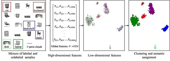
The workflow of the proposed method in four parts is shown in Figure 1. In the classification preparation stage, unlike current deep learning methods, many unlabeled point clouds are mixed with few labeled point clouds to obtain a labeled–unlabeled mixed point cloud set. Next, a deep learning framework is used to extract the mixed features. Then, manifold learning is utilized for simple feature representation by mapping from a high-dimensional space to a low-dimensional space. Finally, an improved clustering algorithm is utilized for semantic assignment in each cluster.
2.1. Mixed Feature Extraction for the Point Clouds of Indoor Components
We adapted PointNet as our backbone to extract point cloud features because PointNet directly processes point clouds and respects the permutation invariance of points in the input. Assume that there are labeled point clouds of indoor components denoted as and unlabeled point clouds denoted as . Let be the mixed point cloud set. Each point cloud consists of n points, and each point is represented by 3 dimensions (x, y, z) [31,42]. If the point cloud is used as the input to extract the feature directly, permutations of the input set are obtained. The framework of feature extraction is primarily composed of a simple symmetric function and a mini-network of a predictive transformation matrix in feature space. This framework can directly extract the global features from an unordered point cloud. This system uses the global max pooling layer as its primary symmetric function. Thus, the framework is invariant to input permutation and will not be affected by an unordered point cloud. Moreover, it contains a spatial transformer network (STN) [31,43] of the predictive transformation matrix in feature space, and learns the transformation matrix from the input points. The dimensions of the transformation matrix are consistent with the feature dimensions. Thus, the matrix is multiplied with the original points to realize the transformation of the input feature space. This framework can be defined as a general function on the point cloud set :
where is a point in each point cloud in . is a continuous function that maps the point cloud set to a matrix. Empirically, is approximated by a multi-layer perceptron and by the composition of a single variable function and the global max pooling function.
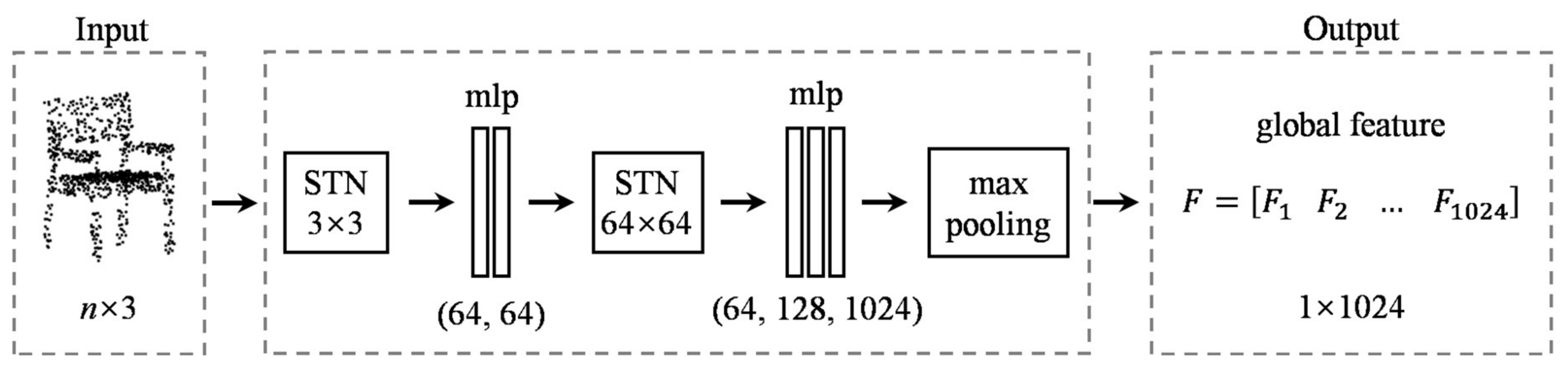
Figure 2 shows the feature extraction structure for a point cloud. The input is a point cloud containing n points. The system predicts a 3 × 3 transformation matrix from the STN. This matrix works on the original points to achieve data alignment. Each point is represented as a 64-dimensional feature by a multi-layer perceptron (mlp) (64, 64) with shared parameters. Then, another alignment network is employed with the point features and predicts a feature transformation matrix to align the features. Further, it uses a three-layer perceptron (64, 128, 1024) for feature extraction, and the dimension of the feature becomes 1024. Finally, it aggregates the point features by the global max pooling layer, and this point cloud can be represented by a 1 × 1024 global feature.
2.2. Dimensionality Reduction for Mixed Features
Although the aforementioned network provides global features, high-dimensional global features have correlation and redundancy [44]. To further alleviate these problems and improve the accuracy and robustness of feature learning, a variety of methods were tested to learn features (such as multiple dimensional scaling [45], principal component analysis [46], locally linear embedding [47], isometric mapping [48], and so on), and the most effective dimensionality reduction method was determined. In this subsection, an automatic feature grouping method based on manifold learning for an embedded dimensionality reduction algorithm is proposed.
Suppose that the high-dimensional global features to be taken are located on a statistical manifold. A probability distribution is used to describe the global features, and the conditional probability distribution function between any two global features in the high-dimensional or low-dimensional space can be obtained. The high-dimensional global features can be defined as (D is the dimension of high-dimensional global features), with N global features. The dimension of every global feature is 1024. There is a (d < D) that has a mapping relationship with F in low-dimensional space, where d is the dimension of the low-dimensional space.
First, the similarity between any two global features is characterized by the conditional probability in the same space. In high-dimensional space, the similarity between and can be expressed as the conditional probability , and the distribution function obeys the Gaussian distribution. The larger is, the higher the similarity between the global features. The global features and in the high-dimensional space are mapped to and in the low-dimensional space. Likewise, the similarity between and can be described as the conditional probability . Mathematically [49], and are given by
where is the variance of the Gaussian distribution [49].
Second, to further explore the distribution correlation between high-dimensional and low-dimensional space, the joint probabilities and are used in the same space, as shown in Equations (4) and (5) [49].
Then, the loss function C is utilized to represent the similarity between the joint probability distribution in low-dimensional space and high-dimensional space. By arbitrarily selecting two global features in the high-dimensional space, the joint probability is given as . Correspondingly, the joint probability in low-dimensional space is . The loss function C is given by [49]
where the Kullback–Leibler divergence () is relative entropy, which is used to measure the similarity of two probabilities in the same event space; and and are the probability distributions of global features in the high-dimensional and low-dimensional spaces, respectively. The loss function C is designed to minimize the distance between and to ensure that the two distributions and have the highest degree of matching. The partial derivative C sub , i.e., the gradient, is calculated. It is then iteratively updated by the gradient descent method until the function values converge. In other words, the matching of the two probability distributions is maximized.
Further, in low-dimensional space, the similarity is expressed using the Student-t distribution for two reasons [49]. First, the distribution of manifold data groups is asymmetrical and heavy-tailed. Second, these data do not entirely obey standard Gaussian distribution. The tail of the t-distribution becomes higher as the degree of freedom increases. When mapping from a high-dimensional space to a low-dimensional space, there is a large distance between the different global features under t-distribution. Hence, the crowding problem is avoided. The gradient has a surprisingly simple form:
Finally, the parameter called “perplexity” is a smooth measure of the effective number of neighbors, , for N global features. The binary search algorithm is used to search for the value of that produces a with a perplexity [49]. This perplexity is defined as
where is the Shannon entropy of used to characterize the uncertainty of the global features; it is also a quantitative indicator of the degree of chaos. The larger the entropy, the greater the confusion.
The pseudocode of the proposed dimension reduction algorithm is shown in Algorithm 1.
| Algorithm 1: Dimensional reduction algorithm. |
| Inputs: A set of global features of point clouds ; perplexity perp; the dimension to be reduced d; number of iterations T, learning rate ; momentum . |
| Compute pairwise affinities with the fixed perplexity perp using (2). |
| Set . |
| Initialize low-dimensional data with |
| Fort = 1 to T do |
| Compute low-dimensional affinities with (5) |
| Compute gradient using (7) |
| Iterative optimization, update low-dimensional data with |
| End for |
| Outputs: A set of low-dimensional features . |
2.3. Semantic Assignment with Few Labeled Samples
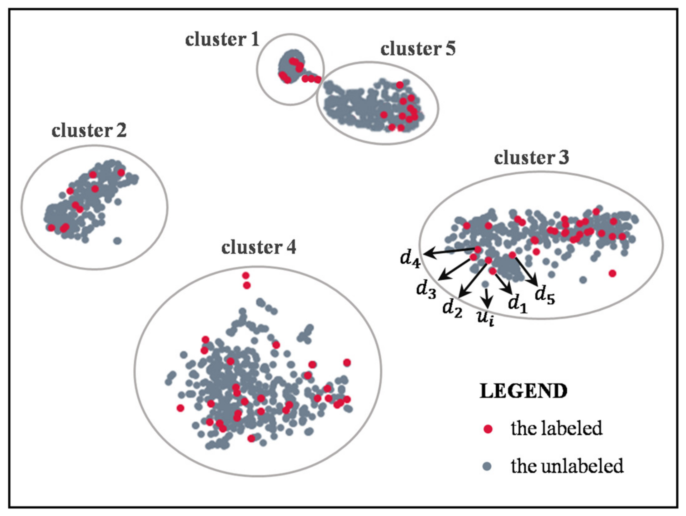
After dimensionality reduction by manifold learning, clustering is combined with a neighborhood search to label the unlabeled point clouds. Clustering is utilized before the neighborhood search instead of directly finding the labeled samples and directly classifying with the neighborhood search for the reasons shown in Figure 3. Taking the 2-D dimensionality reduction result as an example, many unlabeled point clouds in cluster 5 are labeled with the few labeled samples in cluster 1 without first applying clustering. Since the relationship between the features of few labeled point clouds and the features of unlabeled point clouds in the feature space cannot be predicted, it is necessary to utilize a clustering algorithm before the neighborhood search.
The strategy of combining clustering and neighborhood search is used in this method. After trying a variety of clustering methods (such as K-means [50], mixture-of Gaussian [51], agglomerative nesting [52], spectral clustering [53] and so on), the clustering algorithm of density-based spatial clustering of applications with noise (DBSCAN) [54] was applied and improved. This method examines the connectivity between samples from the perspective of sample density, and continuously expands the clusters based on reachable samples to obtain the final clustering results. This clustering algorithm assumes that the clustering structure can be determined by the tightness of the sample distribution, and clusters of various shapes and sizes are found in the samples with noise. This algorithm has been proven to achieve excellent results in both spherical data clustering and non-spherical data clustering [54]. However, these cluster labels are not the semantic labels required by the unlabeled point clouds. Thus, neighborhood search is employed to improve the clustering algorithm to complete the semantic assignment.
Assume that the result of dimensionality reduction is used as the input sample set of the clustering algorithm. There are two thresholds that describe the closeness of the samples in the neighborhood. One is the distance threshold of the neighborhood, and the other is the threshold of the number of samples in the neighborhood.
An arbitrary sample is selected at first, and all neighbors with a distance less than or equal to from are determined. If the number of neighbors is less than , is marked as noise. If the number of neighbors is greater than or equal to , is marked as a core sample, and a new cluster label is assigned. Second, all the neighbors of are traversed. If they are yet unlabeled, the new cluster label of is assigned to them. If they are core samples, their neighbors are traversed in turn, and so on. The cluster gradually grows until there are no more core samples within . Then, an unvisited sample is selected. The same process is then repeated until all samples in are visited. Subsequently, each cluster is traversed. The unlabeled objects and labeled objects are then selected in . Next, is traversed. For each , five labeled objects closest to in are found. The labels of these five labeled objects are recorded as . As shown in Figure 3, taking as an example, comprises all grey dots, and comprises all red dots. The in will choose the closest five labeled objects, which are labeled . Finally, the unlabeled is assigned the label that most frequently occurs in .
The pseudocode of the semantic assignment algorithm is presented in Algorithm 2.
| Algorithm 2: Semantic assignment algorithm | |
| Inputs: A set of samples ; neighborhood parameter and . | |
| Initialize as unvisited, , k = 0, | Add to |
| For in do | End if |
| Mark as visited, determine the neighbors of | End for |
| If then | End if |
| Mark as noise | End for |
| Else | For in do |
| Create new cluster , add to | Determine a set of the labeled samples , and |
| For in do | a set of the unlabeled samples |
| If is not visited then | For in do |
| Mark as visited | Find five labeled samples nearest to in , |
| If then | and take their labels as |
| = | Determine the label that appears the |
| End if | most in , add to |
| End if | End for |
| If not yet a member of any cluster | End for |
| Outputs: Semantic labels | |
3. Experiments
For performance assessment of the proposed method, experiments using open-source datasets were designed and implemented, and the results were evaluated with the evaluation criteria.
3.1. Experimental Data
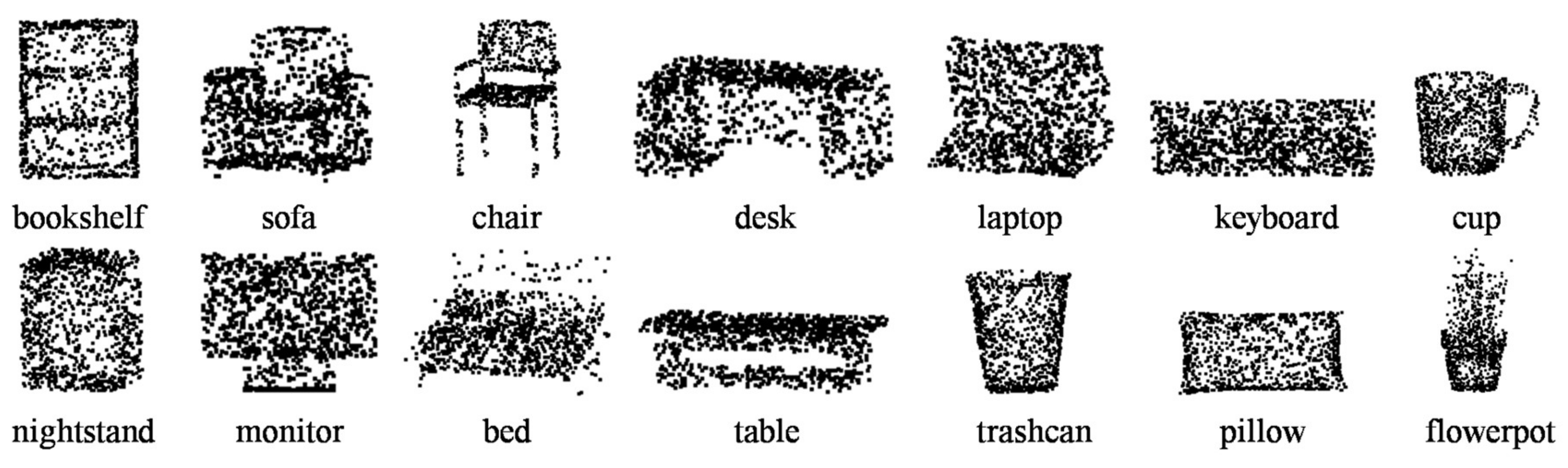
The experimental point clouds were derived from some of the indoor components in the open-source datasets ShapeNetCore [55] and ModelNet40 [27]. Because current deep learning classification networks were selected as baseline methods, the objects of the two datasets were combined to ensure the presence of sufficient training samples. As not all objects in ModelNet40 and ShapeNetCore belong to the components in the indoor scenarios, not all components involved in these two datasets were employed in the experiments. Fourteen categories of components were chosen, as shown in Figure 4, to form a new dataset for the experiments. The remaining categories were used for the pre-training of the feature extraction network in our method. Thus, the point clouds used for the pre-trained feature extraction network did not duplicate the categories used in the experiments.
The new dataset was divided into three parts: the labeled set, the unlabeled set (test set), and the training set, as shown in Table 1. The labeled set consisted of few labeled point clouds which were randomly selected from each class in the new dataset. The proposed method used the labeled set and unlabeled set (test set). In contrast, the baseline methods used the training set and the test set (unlabeled set) for the comparative experiments. As shown in Table 1, the number of labeled objects used in our method is far less than the number of objects used for training by deep learning methods.
3.2. Design of Experiments
The experiments were then designed using the new dataset. First, every selected component was sampled into a point cloud consisting of 1024 points. Next, three different indoor scenarios (office, living room, and bedroom) were selected, with six typical categories in each for the experiments. Additionally, all categories were merged, and a comprehensive classification experiment of the 14 categories was performed. The statistics of the categories for each experiment are shown in Table 2. These three indoor scenarios are typical areas where human activities are frequently engaged in and cover common categories of indoor components. Some categories have unique scene attributes. This comprehensive experiment can show the applicability of the method in complex indoor scenes. Finally, semantic classification was performed for each experiment according to the method described in Section 2. To compare the advantages and disadvantages of the proposed method, PointNet [31], PointNet++ [33], and PointCNN [34] were used. During execution, point clouds with the number of training fields shown in Table 1 were used to train for these three deep learning methods. Then, our method and the baseline methods were used to test the unlabeled/test data.
All the experiments were based on the deep learning framework, Tensorflow [58], and performed on a Dell workstation with an Intel Xeon E5-2630 v3 CPU, NVIDIA GTX-1080Ti GPU (11 GB memory) and 32 GB RAM. The workstation’s operating system was Ubuntu 16.04. We trained the network using a batch size of 32 for 250 epochs, with an initial learning rate of 0.001 and exponential decay of 0.7 after each epoch. Moreover, 3D coordinate information was used as the network input.
4. Experimental Results and Analyses
In this section, we report the extensive experiments that were conducted in different indoor scenarios to evaluate the performance of the proposed method. The effectiveness of the proposed method was verified by carrying out a comprehensive comparison with several 3D point cloud classification methods based on deep learning.
4.1. Experiment 1: Office Scenario
A bookshelf, chair, cup, table, keyboard, and laptop are common components in an office scenario. Therefore, this experiment was mainly used to verify the applicability of the proposed method for the semantic classification of typical components in an office scenario. Figure 5 shows the confusion matrices for the predictions of all methods on the unlabeled set (test set) in the office scenario. Every 6 × 6 matrix exhibits the results of the framework predictions. The rows were equal to the true labels of the point clouds, while the columns corresponded to the predicted labels. The value of each element in the confusion matrix was the number of predictions of the samples in a class corresponding to each column, and the true labels of these samples were represented by the row. The diagonal elements in the matrix represent the number of samples that were predicted as the correct class for each class, and the off-diagonal elements show the predicted errors. The performance shows that, in an office scenario, our method based on a small number of labeled samples can effectively capture the salient features of point clouds, as it has a relatively small number of errors and can obtain better results than the baseline methods.
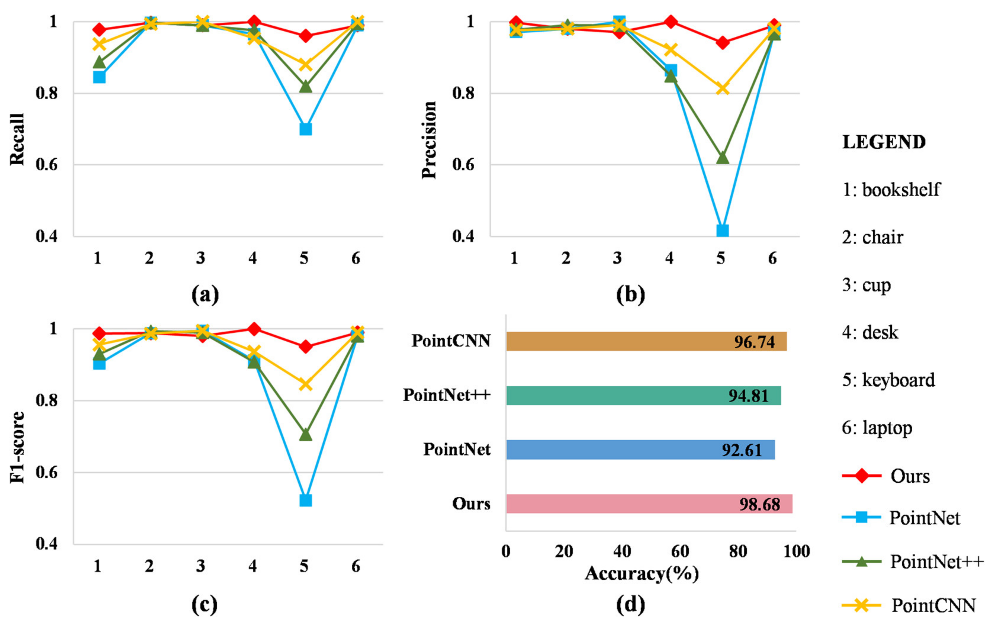
Figure 6 displays the results of the quantitative assessment of all methods in the office scenario using recall, precision, score, and accuracy. It can be seen from Figure 6a–c that the four methods’ predictions of the three categories of chair, cup, and laptop were similar. For the other categories, there were differences among the methods. The recall, precision, and scores of each class in our approach were slightly higher than those under the baseline methods. The three measurements of the keyboard were better than the other methods because the baseline methods confused the keyboard with the bookshelf, desk, and laptop. As seen in Figure 6d, comparing our proposed method with the baseline methods, our approach offers improved accuracy of 6.07% (PointNet), 3.87% (PointNet++), and 1.94% (PointCNN). This experiment thus validates the applicability of the proposed method in an office scenario.
4.2. Experiment 2: Living Room Scenario
A flowerpot, monitor, pillow, sofa, table, and trashcan are typical components in a living room scenario. Therefore, this experiment was mainly used to verify the applicability of the proposed method for the semantic classification of typical components in a living room scenario. The confusion matrices for the predictions of all methods on the unlabeled set (test set) in the living room are shown in Figure 7. These four 6 × 6 confusion matrices display the point cloud prediction results. Clearly, there were fewer errors in our framework than the baseline methods. This suggests that our method can effectively capture the distinguishing features of point clouds. It was particularly difficult for the baseline methods to correctly classify the table and the trashcan. Moreover, baseline methods confused the table with the flowerpot, monitor, and trashcan, while the trashcan was confused with the flowerpot.
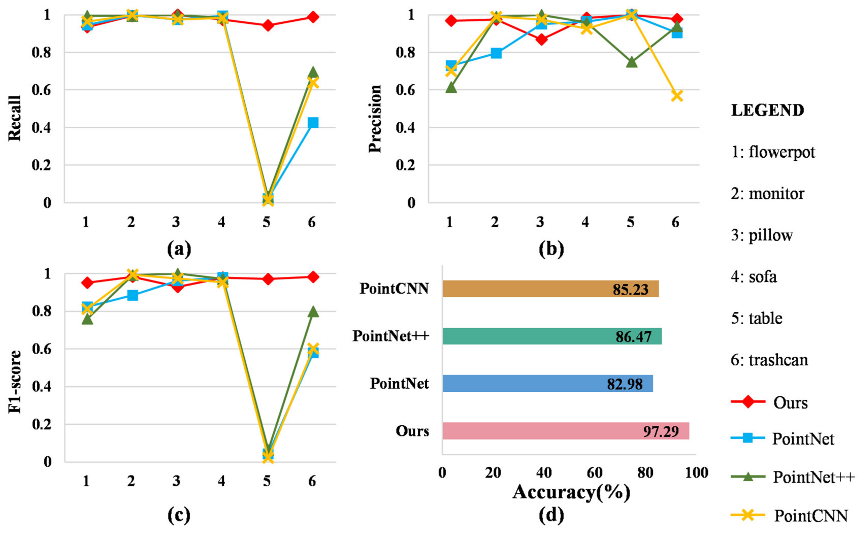
As is clearly shown in Figure 8, the four measurements of these methods were recorded to assess the classification results. These three measurements (recall, precision, and score) of our method for most categories remained at a relatively high level that was higher than the baseline methods, specifically for the table. The baseline methods regarded the table as a monitor, flowerpot, or trashcan. Similarly, our method predicted the flowerpot and table as a pillow; thus, the precision of the pillow in our method was lower than that under the baseline methods. For accuracy, compared with the baseline methods, our method achieved the best performance with an accuracy of 97.29%. The most accurate baseline method was PointNet++, with an accuracy of 86.47%, which was 10.82% lower than our method. Our approach outperformed PointNet by 14.31% and PointCNN by 12.06%. This shows that the proposed method had the best applicability in a living room scenario.
4.3. Experiment 3: Bedroom Scenario
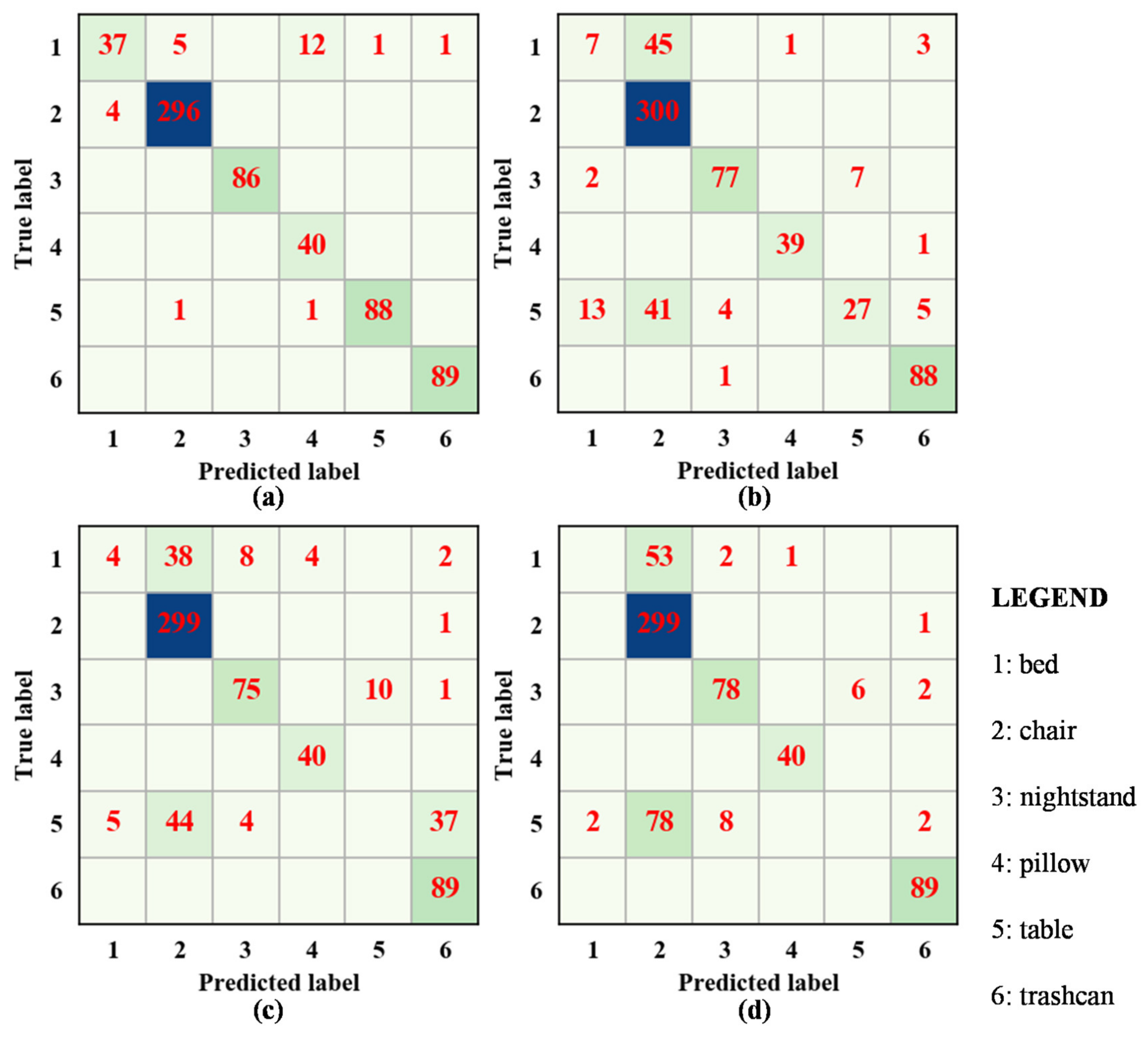
Typically, a bed, chair, nightstand, pillow, table, and trashcan are common components in a bedroom scenario. Therefore, this experiment was mainly used to verify the applicability of the proposed method for the semantic classification of typical components in a bedroom scenario. Figure 9 shows the confusion matrices of all methods on the unlabeled set (test set) in the bedroom scenario. Among the four methods, our method had the fewest errors. Notably, it identified the components of the bed and table relatively correctly, while the baseline methods incorrectly identified the bed as a chair, nightstand, pillow, or trashcan, and recognized the table as a bed, chair, nightstand, or trashcan (or failed to recognize the table entirely).
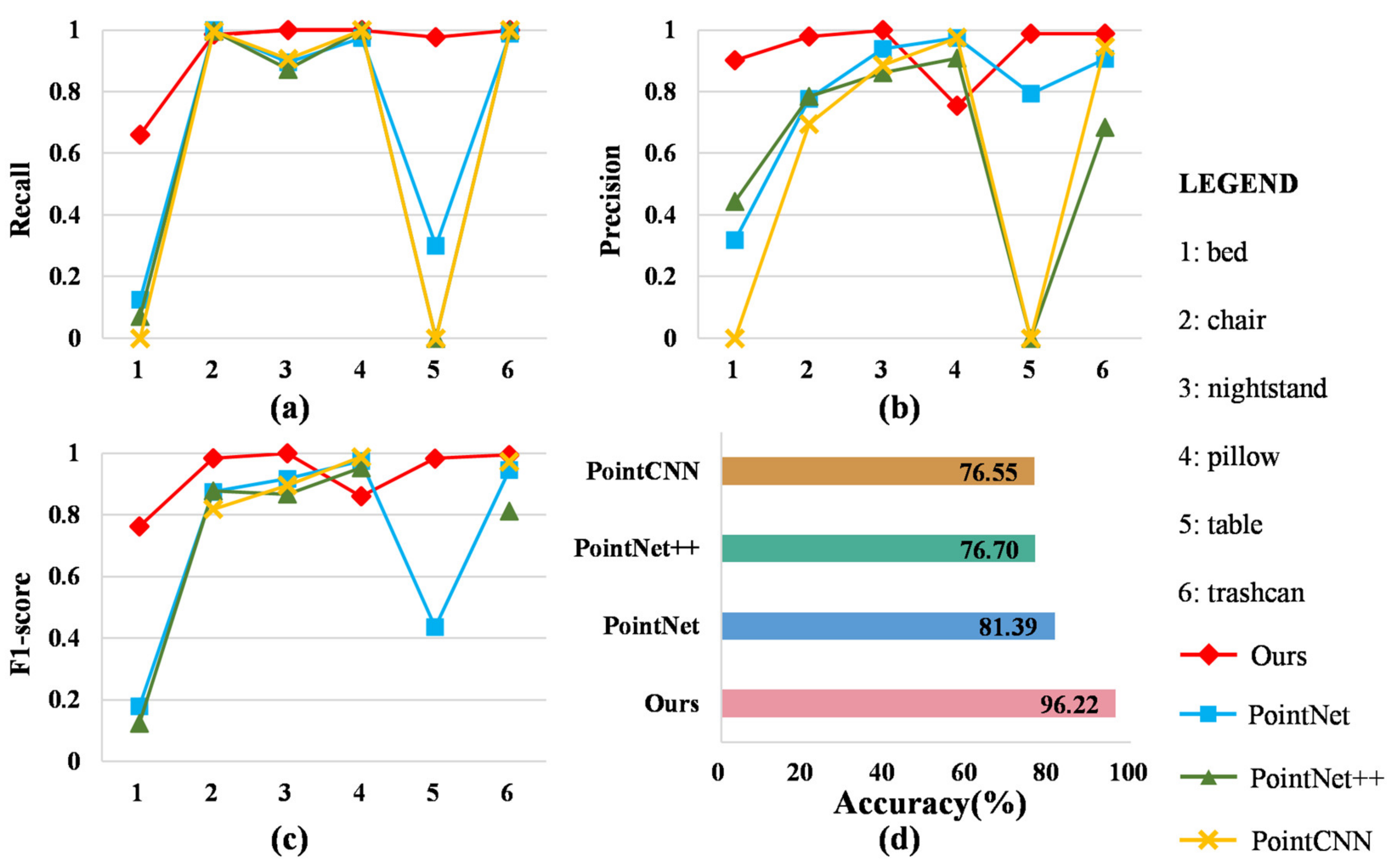
Four measurements were recorded in Figure 10. As can be seen, our approach achieved superior performance compared to the baseline approaches, especially for the bed, nightstand, and table. Just as PointNet++ did not recognize the table, PointCNN did not recognize the bed and table, so the corresponding recall and precision were zero. Although the proposed method provided good performance in the prediction of the bed, the precision and scores of the pillow were lower than those of other methods because this method predicted part of the bed as a pillow. The most accurate baseline method was PointNet with an accuracy of 81.39%. Our method offered the best accuracy of 96.22% compared with the baseline methods. Our approach significantly outperformed PointNet by 14.83%. This experiment suggests that the proposed method has good applicability in the bedroom scenario.
4.4. Experiment 4: Comprehensive Classification
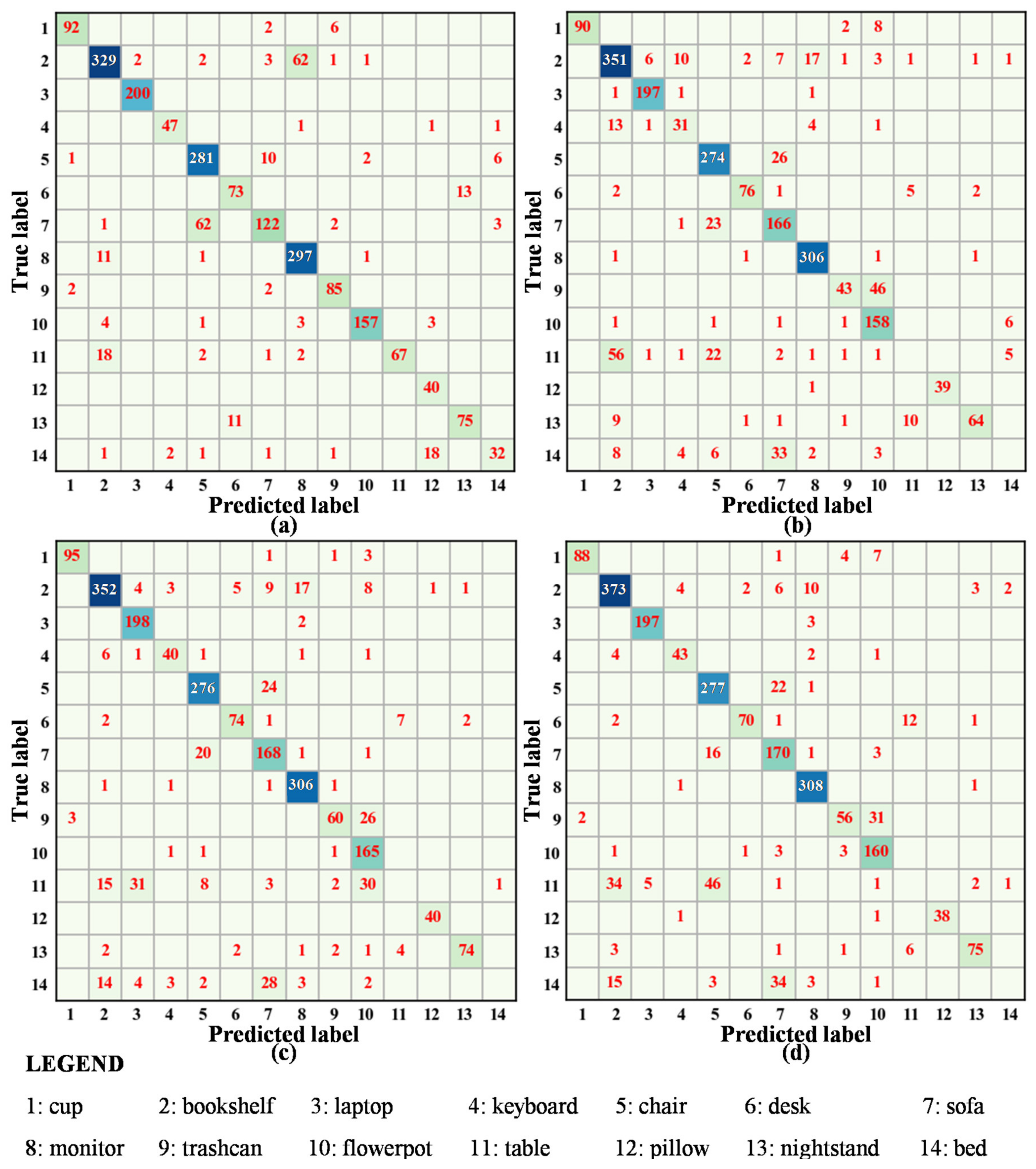
To further explore the proposed method, a comprehensive complex indoor scenario was simulated. The four methods were used to classify all categories in the new dataset, and the results were recorded, as shown in Figure 11. The baseline methods classified the table and bed improperly. Conversely, our proposed method could correctly identify each category. Due to similarities in their geometric structures, our method was slightly confused in distinguishing the table and the bed (e.g., the bookshelf and monitor, chair and sofa, desk and nightstand, and table and bookshelf). Nevertheless, compared to the baseline methods, the proposed method still obtained better classification results in this experiment because it could accurately predict the table and bed.
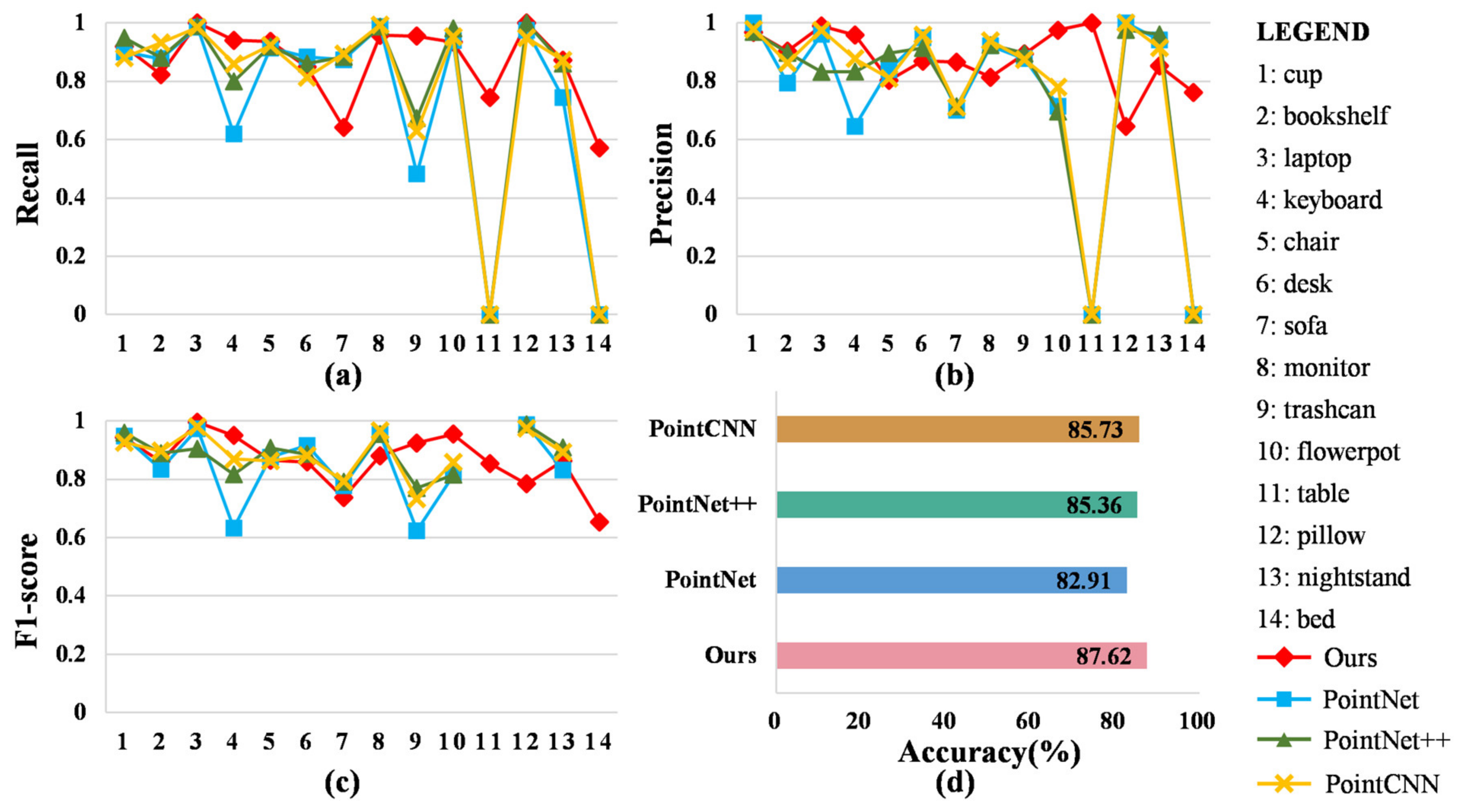
The performance of all approaches is provided in Figure 12. For our approach, each category was predicted relatively accurately with better performance than the baseline approaches. However, the number of correctly predicted bookshelf, sofa, and monitor objects was lower than the baseline methods. Hence, the recall of the bookshelf, sofa, and monitor was also lower than other methods. Moreover, some beds were misclassified as pillows, resulting in a lower precision for the pillow than that achieved by the baseline methods. However, for the baseline methods, the table and bed were predicted like other categories, resulting in zero recall and precision. Therefore, the accuracy of our method was higher than that of the baseline methods. PointCNN had the highest accuracy among the baseline methods, with an accuracy of 85.73%. The accuracy of our approach was 87.62%, which was higher than that of PointCNN by 1.89%. These results demonstrate that even under a comprehensive complex indoor scenario, the proposed method remains practical.
5. Discussion
5.1. Influence of the Dimensionality Reduction and Clustering on the Accuracy
In dimensionality reduction and semantic assignment, the classification accuracy is affected by the algorithms of dimensionality reduction and clustering. Various algorithms of dimensionality reduction (such as multiple dimensional scaling [45], principal component analysis [46], locally linear embedding [47], isometric mapping [48] and T-distributed stochastic neighbor embedding [49]) and clustering algorithms (such as K-means [50], mixture-of Gaussian [51], agglomerative nesting [52], spectral clustering [53] and density-based spatial clustering of applications with noise [54]) were tried. After many comparisons, the methods with best performance were chosen. Most of the dimensional reduction algorithms learned the similarity between the features poorly in the high-dimensional space, so they failed to distinguish the different features in the low-dimensional space. Moreover, the shape of each cluster in the low-dimensional space was various, and compared to other clustering methods, DBSCAN performed better in this respect.
5.2. Influence of the Geometric Contrast on the Classification Accuracy
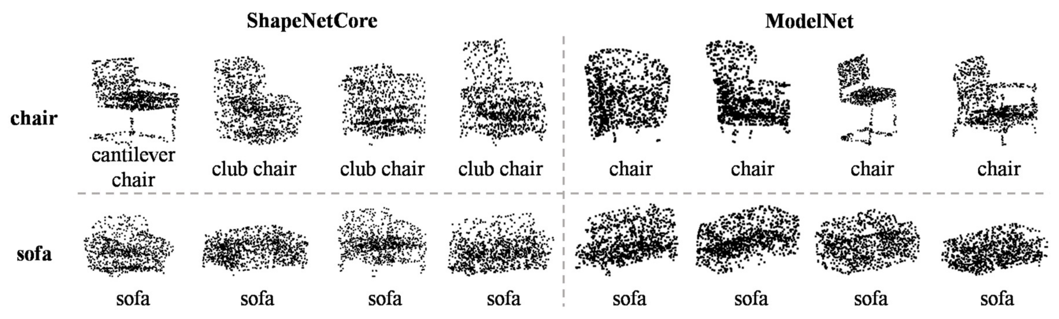
In reality, objects in different scenarios have more varied types and are more structurally complex in indoor scenarios. There are both similarities and dissimilarities among the geometric structures of different classes of objects. Similar geometric structures of several categories of objects will increase the difficulty in correctly distinguishing those objects during classification (for both the proposed and baseline methods). Consider the chair and sofa in the fourth experiment as an example (as shown in Figure 13). In open-source datasets such as ShapeNetCore and ModelNet40, the structures of some sofas and chairs are very similar. For the proposed method, the semantics of some objects in the datasets are too close, which increases the difficulty of classification. Hence, establishing a strict semantic system for indoor scene components is required to reduce the overlap among different categories of indoor components for semantics. Further, the existing indoor components’ point clouds require semantic standardization according to the semantic system.
5.3. Influence of the Semantic Assignment Parameters on Classification Accuracy
In the semantic assignment stage, the classification accuracy was affected by , and the number of nearest neighbors. During the experiments, and were determined by visualizing clustering results in two-dimensional space. Different experiments had different values of and . In the future work, we will try to determine the two thresholds using an effective adaptive method. To study the relationship between the classification accuracy of the proposed method and the number of nearest neighbors, we conducted more extensive research. Different numbers of nearest neighbors (1, 3, 5, 7, 9) were selected to verify their impact on classification accuracy in experiment 4.
Table 3 lists the distinct classification accuracy values corresponding to different nearest neighbors. When the value of the nearest neighbor parameter ranged from 1 to 9, the accuracy fluctuated within about 1%. The highest accuracy was 87.62% at 5. Meanwhile, the parameter of nearest neighbors had different optimal values in different experiments. If there was significant variation among the geometrical structures of several categories, the number of nearest neighbors had only a slight effect on the classification results.
5.4. Robustness in Point Density
Another critical issue for the robustness of our framework is addressed in this subsection. In practice, dealing with point clouds with different densities is a common situation. Under such circumstances, it is important to investigate the robustness and generalization ability of the framework in different density situations.
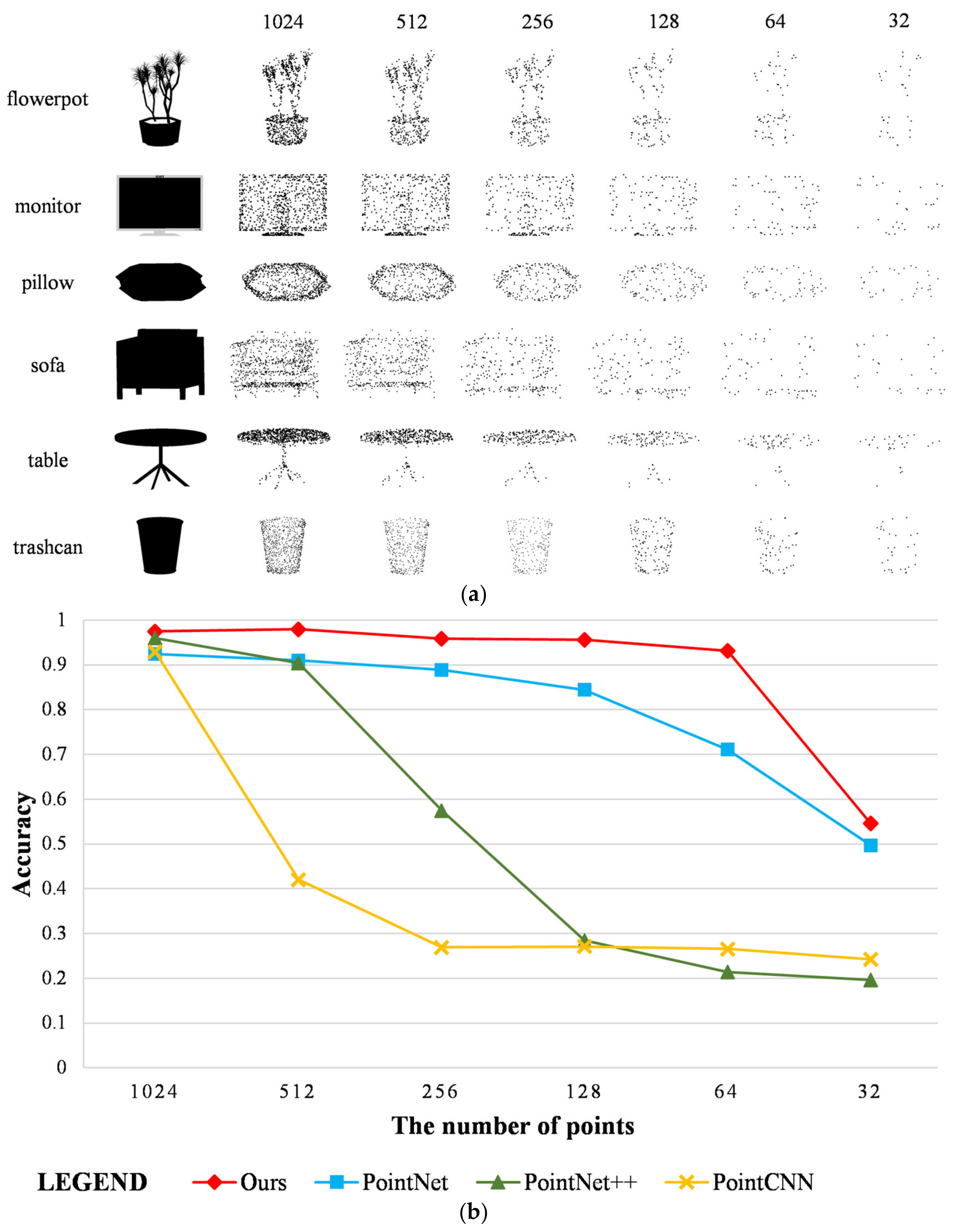
The point clouds of indoor components were sampled into different points in the living room scenario. The number of employed points was selected as 32, 64, 128, 256, 512, and 1024, respectively (as shown in Figure 14a). The proposed method was compared with the baseline methods. The classification results are shown in Figure 14b. It was observed that data of different densities can significantly reduce the performance of PointCNN and PointNet++. For instance, when there are 512 points, the accuracy of PointCNN decreases by about 50%; when 256 points are available, the accuracy of PointNet++ is lower than 60%. The classification accuracy of PointNet decreases with the number of input points. The proposed method has a synchronous downward trend with PointNet, but the accuracy is higher. Our method remains stable under different point densities. When the number of input points is 1024, 512, 256, and 128, the overall accuracy is maintained at 95%. Here, the system maintains relatively good performance and only drops by about 2% when 64 points are used for testing the accuracy, while the accuracy of the PointNet drops by about 13%. There are two reasons for this stability: one is that the parameters of our feature extraction framework are more accurately able to discriminate between point cloud features than the baseline methods; the other is that dimensionality reduction and semantic assignment can distinguish similar features from dissimilarities according to feature consistency. This effectively reduces the impact of point clouds with different densities. The experimental results and comparisons demonstrate the point density robustness of our method.
5.5. Number of Categories of Labeled Samples
As shown in Figure 3, if the categories of the point clouds to be classified are known, they can be directly classified using few labeled point clouds of the known categories. For a new task of point cloud classification, our method uses open-source dataset for pre-training. Then, just a few labeled point clouds in each category can achieve effective classification for this specific task. However, for the existing deep learning methods, it is necessary to label sufficient point clouds per class for training in this specific task. This process takes time and effort. If the categories of the point clouds to be classified are unknown, as many categories of point clouds as possible should be labeled. This is required for all classification methods. Classification methods based on deep learning require a sufficient number of labeled point clouds with various categories. Our method differs from previous methods in that only a few labeled point clouds in each category are labeled here.
6. Conclusions
In this study, a novel classification method of point clouds for indoor components using few labeled samples was proposed. The novelty of this method lies in: (1) mixing few labeled samples with a large number of unlabeled samples to extract mixed features; and (2) using few labeled samples to achieve classification through the dimensionality reduction algorithm based on manifold learning and semantic label assignment. This method reduces the difficulty of quantifying the similarities and differences of point cloud features and effectively distinguishes similar features from dissimilar features. It can achieve point cloud classification using only a few labeled samples. In the four experiments—three single-attribute indoor scenarios and one comprehensive complex indoor scenario—the results indicate that the proposed method not only has higher classification accuracy but also reduces the cost of labeling the training samples. Compared with existing deep learning methods, the proposed method does not separate the training set from the test set when classifying and only requires few labeled samples to achieve classification. Furthermore, it has a higher generalization ability. For any classification task, only two conditions are required. The first is to train the framework using an open-source dataset similar to the classified object, and the second is to label a small number of multi-class samples to be classified. Therefore, the proposed method is suitable for many classification tasks using open-source datasets.
Although the classification results of the proposed method were good in typical indoor scenarios, these categories do not cover all indoor components. For future studies, we will attempt to classify more categories of components to simulate real complex indoor scenarios. The proposed method extracts global features for classification. Thus, we will focus on further optimizing the network structure (such as introducing an attention mechanism, tensor, etc.) to extract local features.
Author Contributions
Conceptualization and methodology, H.W., H.Y., and S.H.; software, H.Y., S.H., and D.Z.; validation, H.Y., D.Z., and C.L.; writing—original draft preparation, H.W. and H.Y.; writing—review and editing, H.W., H.Y., and S.H.; visualization, H.Y. and D.Z.; supervision, C.L., H.Z., C.G., and L.C.; funding acquisition, H.W. All authors have read and agreed to the published version of the manuscript.
Funding
This research was supported and funded by the National Key Research and Development Program of China (Grant No. 2018YFB1305000), (Grant No. 2016YFB0502104), the National Natural Science Foundation of China (Grant No. 41671451) and the Fundamental Research Funds for the Central Universities of China (Grant No. 22120190195).
Acknowledgments
The authors thank the anonymous reviewers for their constructive suggestions. The authors thank Rui Bu for his help in debugging the code of PointCNN. We are also grateful to Shoujun Jia, Zeran Xu, Akram Akbar, and Qian Liu for their advice and support in the experimental design.
Conflicts of Interest
The authors declare no conflict of interest.
References
- Chang, H.J.; Lee, C.S.G.; Lu, Y.H.; Hu, Y.C. P-SLAM: Simultaneous localization and mapping with environmental-structure prediction. IEEE Trans. Robot. 2007, 23, 281–293. [Google Scholar] [CrossRef]
- Weingarten, J.W.; Gruener, G.; Siegwart, R. A state-of-the-art 3D sensor for robot navigation. In Proceedings of the 2004 IEEE/RSJ International Conference on Intelligent Robots and Systems (IROS) (IEEE Cat. No.04CH37566), Sendai, Japan, 28 September–2 October 2004; Volume 3, pp. 2155–2160. [Google Scholar] [CrossRef] [Green Version]
- Endres, F.; Hess, J.; Sturm, J.; Cremers, D.; Burgard, W. 3-D Mapping With an RGB-D Camera. IEEE Trans. Robot. 2014, 30, 177–187. [Google Scholar] [CrossRef]
- Bassier, M.; Vergauwen, M. Topology Reconstruction of BIM Wall Objects from Point Cloud Data. Remote Sens. 2020, 12, 1800. [Google Scholar] [CrossRef]
- Tashakkori, H.; Rajabifard, A.; Kalantari, M. A new 3D indoor/outdoor spatial model for indoor emergency response facilitation. Build. Environ. 2015, 89, 170–182. [Google Scholar] [CrossRef]
- Fernández-Caramés, C.; Serrano, F.J.; Moreno, V.; Curto, B.; Rodríguez-Aragón, J.F.; Alves, R. A real-time indoor localization approach integrated with a Geographic Information System (GIS). Robot. Auton. Syst. 2016, 75, 475–489. [Google Scholar] [CrossRef]
- Musialski, P.; Wonka, P.; Aliaga, D.G.; Wimmer, M.; van Gool, L.; Purgathofer, W. A Survey of Urban Reconstruction. Comput. Graph. Forum 2013, 32, 146–177. [Google Scholar] [CrossRef]
- Tran, H.; Khoshelham, K. Procedural Reconstruction of 3D Indoor Models from Lidar Data Using Reversible Jump Markov Chain Monte Carlo. Remote Sens. 2020, 12, 838. [Google Scholar] [CrossRef] [Green Version]
- Liu, W.; Sun, J.; Li, W.; Hu, T.; Wang, P. Deep Learning on Point Clouds and Its Application: A Survey. Sensors (Basel) 2019, 19, 4188. [Google Scholar] [CrossRef] [Green Version]
- Grilli, E.; Menna, F.; Remondino, F. A review of point clouds segmentation and classification algorithms. Int. Arch. Photogramm. Remote Sens. Spatial Inf. Sci. 2017, 2, 339–344. [Google Scholar] [CrossRef] [Green Version]
- Luo, H.; Wang, C.; Wen, Y.; Guo, W. 3-D Object Classification in Heterogeneous Point Clouds via Bag-of-Words and Joint Distribution Adaption. IEEE Geosci. Remote Sens. Lett. 2019, 1–5. [Google Scholar] [CrossRef]
- Yu, Y.; Li, J.; Guan, H.; Wang, C. Automated Extraction of Urban Road Facilities Using Mobile Laser Scanning Data. IEEE Trans. Intell. Transp. Syst. 2015, 16, 2167–2181. [Google Scholar] [CrossRef]
- Song, Y.F.; Chen, X.W.; Li, J.; Zhao, Q.P. Embedding 3D Geometric Features for Rigid Object Part Segmentation. In Proceedings of the 2017 IEEE International Conference on Computer Vision (ICCV), Venice, Italy, 22–29 October 2017; pp. 580–588. [Google Scholar] [CrossRef]
- Wang, X.G.; Zhou, B.; Wang, Z.J.; Zou, D.Q.; Chen, X.W.; Zhao, Q.P. Efficiently consistent affinity propagation for 3D shapes co-segmentation. Visual Comput. 2018, 34, 997–1008. [Google Scholar] [CrossRef]
- Guo, Y.L.; Bennamoun, M.; Sohel, F.; Lu, M.; Wan, J.W. 3D Object Recognition in Cluttered Scenes with Local Surface Features: A Survey. IEEE Trans. Pattern Anal. 2014, 36, 2270–2287. [Google Scholar] [CrossRef]
- Chen, H.; Bhanu, B. 3D free-form object recognition in range images using local surface patches. Int. Conf. Patt. Recog. 2004, 3, 136–139. [Google Scholar] [CrossRef]
- Johnson, A.E.; Hebert, M. Using spin images for efficient object recognition in cluttered 3D scenes. IEEE Trans. Pattern Anal. 1999, 21, 433–449. [Google Scholar] [CrossRef] [Green Version]
- Sun, J.A.; Ovsjanikov, M.; Guibas, L. A Concise and Provably Informative Multi-Scale Signature Based on Heat Diffusion. Comput. Graph. Forum 2009, 28, 1383–1392. [Google Scholar] [CrossRef]
- Rusu, R.B.; Blodow, N.; Marton, Z.C.; Beetz, M. Aligning Point Cloud Views using Persistent Feature Histograms. In Proceedings of the 2008 IEEE/RSJ International Conference on Intelligent Robots and Systems, Nice, France, 22–26 September 2008; pp. 3384–3391. [Google Scholar] [CrossRef]
- Rusu, R.B.; Blodow, N.; Beetz, M. Fast Point Feature Histograms (FPFH) for 3D Registration. In Proceedings of the 2009 IEEE International Conference on Robotics and Automation, Kobe, Japan, 12–17 May 2009; pp. 1848–1853. [Google Scholar] [CrossRef]
- Secord, J.; Zakhor, A. Tree detection in urban regions using aerial lidar and image data. IEEE Geosci. Remote Sens. Lett. 2007, 4, 196–200. [Google Scholar] [CrossRef]
- Li, N.; Pfeifer, N.; Liu, C. Tensor-Based Sparse Representation Classification for Urban Airborne LiDAR Points. Remote Sens. 2017, 9, 1216. [Google Scholar] [CrossRef] [Green Version]
- Manevitz, L.M.; Yousef, M. One-Class SVMs for Document Classification. J. Mach. Learn. Res. 2001, 2, 139–154. [Google Scholar]
- Garcia-Gutierrez, J.; Gonçalves-Seco, L.; Riquelme-Santos, J.C.; Alegre, R.C. Decision trees on lidar to classify land uses and covers. In Proceedings of the ISPRS Workshop: Laser Scanning, Enschede, The Netherlands, 12–14 September 2005; pp. 323–328. [Google Scholar]
- Barros, R.C.; Basgalupp, M.P.; de Carvalho, A.C.P.L.F.; Freitas, A.A. A Survey of Evolutionary Algorithms for Decision-Tree Induction. IEEE Trans. Syst. Man Cybern. C 2012, 42, 291–312. [Google Scholar] [CrossRef] [Green Version]
- Breiman, L. Random forests. Mach. Learn. 2001, 45, 5–32. [Google Scholar] [CrossRef] [Green Version]
- Zhirong, W.; Song, S.; Khosla, A.; Fisher, Y.; Linguang, Z.; Xiaoou, T.; Xiao, J. 3D ShapeNets: A deep representation for volumetric shapes. In Proceedings of the 2015 IEEE Conference on Computer Vision and Pattern Recognition (CVPR), Boston, MA, USA, 7–12 June 2015; pp. 1912–1920. [Google Scholar] [CrossRef] [Green Version]
- Maturana, D.; Scherer, S. VoxNet: A 3D Convolutional Neural Network for real-time object recognition. In Proceedings of the 2015 IEEE/RSJ International Conference on Intelligent Robots and Systems (IROS), Hamburg, Germany, 28 September–2 October 2015; pp. 922–928. [Google Scholar] [CrossRef]
- Shi, B.; Bai, S.; Zhou, Z.; Bai, X. DeepPano: Deep Panoramic Representation for 3-D Shape Recognition. IEEE Signal Process. Lett. 2015, 22, 2339–2343. [Google Scholar] [CrossRef]
- Su, H.; Maji, S.; Kalogerakis, E.; Learned-Miller, E. Multi-view Convolutional Neural Networks for 3D Shape Recognition. In Proceedings of the 2015 IEEE International Conference on Computer Vision (ICCV), Santiago, Chile, 7–13 December 2015; pp. 945–953. [Google Scholar] [CrossRef] [Green Version]
- Charles, R.Q.; Su, H.; Kaichun, M.; Guibas, L.J. PointNet: Deep Learning on Point Sets for 3D Classification and Segmentation. In Proceedings of the 2017 IEEE Conference on Computer Vision and Pattern Recognition (CVPR), Honolulu, HI, USA, 21–26 July 2017; pp. 177–185. [Google Scholar] [CrossRef] [Green Version]
- Griffiths, D.; Boehm, J. A Review on Deep Learning Techniques for 3D Sensed Data Classification. Remote Sens. 2019, 11, 1499. [Google Scholar] [CrossRef] [Green Version]
- Qi, C.R.; Yi, L.; Su, H.; Guibas, L. PointNet++: Deep Hierarchical Feature Learning on Point Sets in a Metric Space. In Proceedings of the 31st Annual Conference on Neural Information Processing Systems, Long Beach, CA, USA, 4–6 December 2017. [Google Scholar]
- Li, Y.; Bu, R.; Sun, M.; Wu, W.; Di, X.; Chen, B. PointCNN: Convolution On X-Transformed Points. In Proceedings of the 31st Annual Conference on Neural Information Processing Systems, Long Beach, CA, USA, 4–6 December 2017. [Google Scholar]
- Chen, L.; Zhan, W.; Tian, W.; He, Y.; Zou, Q. Deep Integration: A Multi-Label Architecture for Road Scene Recognition. IEEE Trans. Image Process. 2019, 28, 4883–4898. [Google Scholar] [CrossRef]
- Chen, L.; Wang, Q.; Lu, X.K.; Cao, D.P.; Wang, F.Y. Learning Driving Models From Parallel End-to-End Driving Data Set. Proc. IEEE 2020, 108, 262–273. [Google Scholar] [CrossRef]
- Mensink, T.; Verbeek, J.; Perronnin, F.; Csurka, G. Metric Learning for Large Scale Image Classification: Generalizing to New Classes at Near-Zero Cost. In Computer Vision—ECCV 2012; Springer: Berlin/Heidelberg, Germany, 2012; pp. 488–501. [Google Scholar]
- Mensink, T.; Verbeek, J.; Perronnin, F.; Csurka, G. Distance-Based Image Classification: Generalizing to New Classes at Near-Zero Cost. IEEE Trans. Pattern Anal. 2013, 35, 2624–2637. [Google Scholar] [CrossRef] [Green Version]
- Cheny, Z.; Fuy, Y.; Zhang, Y.; Jiang, Y.G.; Xue, X.; Sigal, L. Multi-level Semantic Feature Augmentation for One-shot Learning. IEEE Trans. Image Process. 2019, 28, 4594–4605. [Google Scholar] [CrossRef] [Green Version]
- Cai, Q.; Pan, Y.W.; Yao, T.; Yan, C.G.; Mei, T. Memory Matching Networks for One-Shot Image Recognition. In Proceedings of the 2018 IEEE/CVF Conference on Computer Vision and Pattern Recognition, Salt Lake City, UT, USA, 18–23 June 2018; pp. 4080–4088. [Google Scholar] [CrossRef] [Green Version]
- Yang, Y.Q.; Feng, C.; Shen, Y.R.; Tian, D. FoldingNet: Point Cloud Auto-encoder via Deep Grid Deformation. 2018 IEEE Conf. Comput. Vis. Pattern Recognit. 2018, 206–215. [Google Scholar] [CrossRef] [Green Version]
- Bello, S.A.; Yu, S.; Wang, C.; Adam, J.M.; Li, J. Review: Deep Learning on 3D Point Clouds. Remote Sens. 2020, 12, 1729. [Google Scholar] [CrossRef]
- Jaderberg, M.; Simonyan, K.; Zisserman, A.; Kavukcuoglu, K. Spatial Transformer Networks. arXiv 2015, arXiv:1506.02025. [Google Scholar]
- Huang, R.; Xu, Y.S.; Hong, D.F.; Yao, W.; Ghamisi, P.; Stilla, U. Deep point embedding for urban classification using ALS point clouds: A new perspective from local to global. ISPRS J. Photogramm. Remote Sens. 2020, 163, 62–81. [Google Scholar] [CrossRef]
- Cox, T.F.; Cox, M.A. Multidimensional Scaling; Chapman & Hall/CRC: London, UK, 1994. [Google Scholar]
- Shen, H.T. Principal Component Analysis. In Encyclopedia of Database Systems; Springer: Berlin/Heidelberg, Germany, 2009. [Google Scholar]
- Roweis, S.T.; Saul, L.K. Nonlinear dimensionality reduction by locally linear embedding. Science 2000, 290, 2323–2326. [Google Scholar] [CrossRef] [PubMed] [Green Version]
- Tenenbaum, J.B.; de Silva, V.; Langford, J.C. A global geometric framework for nonlinear dimensionality reduction. Science 2000, 290, 2319–2323. [Google Scholar] [CrossRef]
- Maaten, L.V.D.; Hinton, G.E. Visualizing Data using t-SNE. J. Mach. Learn. Res. 2008, 9, 2579–2605. [Google Scholar]
- Hartigan, J.A.; Wong, M.A. Algorithm AS 136: A K-Means Clustering Algorithm. Appl. Stat. 1979, 28, 100. [Google Scholar] [CrossRef]
- He, X.F.; Cai, D.; Shao, Y.L.; Bao, H.J.; Han, J.W. Laplacian Regularized Gaussian Mixture Model for Data Clustering. IEEE Trans. Knowl. Data Eng. 2011, 23, 1406–1418. [Google Scholar] [CrossRef] [Green Version]
- Fox, W.R.; Kaufman, L.; Rousseeuw, P.J. Finding Groups in Data: An Introduction to Cluster Analysis. Appl. Stat. 1991, 40, 486. [Google Scholar] [CrossRef]
- Von Luxburg, U. A tutorial on spectral clustering. Stat. Comput. 2007, 17, 395–416. [Google Scholar] [CrossRef]
- Ester, M.; Kriegel, H.-P.; Sander, J.; Xu, X. A Density-Based Algorithm for Discovering Clusters in Large Spatial Databases with Noise. KDD ‘96 1996, 96, 226–231. [Google Scholar]
- Chang, A.X.; Funkhouser, T.A.; Guibas, L.J.; Hanrahan, P.; Huang, Q.-X.; Li, Z.; Savarese, S.; Savva, M.; Song, S.; Su, H.; et al. ShapeNet: An Information-Rich 3D Model Repository. arXiv 2015, arXiv:1512.03012. [Google Scholar]
- Luciano, L.; Ben Hamza, A. Deep similarity network fusion for 3D shape classification. Vis. Comput. 2019, 35, 1171–1180. [Google Scholar] [CrossRef]
- Liu, C.; Zeng, D.D.; Wu, H.B.; Wang, Y.; Jia, S.J.; Xin, L. Urban Land Cover Classification of High-Resolution Aerial Imagery Using a Relation-Enhanced Multiscale Convolutional Network. Remote Sens. 2020, 12, 311. [Google Scholar] [CrossRef] [Green Version]
- Steckel, J.; Boen, A.; Peremans, H. Broadband 3-D Sonar System Using a Sparse Array for Indoor Navigation. IEEE Trans. Robot. 2013, 29, 161–171. [Google Scholar] [CrossRef]
Figure 1.
Workflow of the proposed point cloud classification. The details of feature extraction, dimensionality reduction, and semantic classification are described in Section 2.1, Section 2.2 and Section 2.3.
Figure 1.
Workflow of the proposed point cloud classification. The details of feature extraction, dimensionality reduction, and semantic classification are described in Section 2.1, Section 2.2 and Section 2.3.

Figure 2.
Architecture of the global feature extraction network. STN: spatial transformer network; mlp: multi-layer perceptron.
Figure 2.
Architecture of the global feature extraction network. STN: spatial transformer network; mlp: multi-layer perceptron.

Figure 3.
An example of clustering in a low-dimensional space. Each dot represents a feature. Each cluster obtained by clustering is marked with a circle.
Figure 3.
An example of clustering in a low-dimensional space. Each dot represents a feature. Each cluster obtained by clustering is marked with a circle.

Figure 4.
A sample point cloud from each category of the new dataset.

Figure 5.
Confusion matrices for the methods on the dataset corresponding to the office scenario: (a) our method, (b) PointNet, (c) PointNet++, and (d) PointCNN. The value of each element in the confusion matrix is the number of samples in each category. The darker the color, the more number of samples in corresponding category.

Figure 6.
Experimental results of the methods on the dataset corresponding to the office scenario: (a) Recall; (b) Precision; (c) score; (d) Accuracy.
Figure 6.
Experimental results of the methods on the dataset corresponding to the office scenario: (a) Recall; (b) Precision; (c) score; (d) Accuracy.

Figure 7.
Confusion matrices for the methods on the dataset corresponding to the living room scenario: (a) our method, (b) PointNet, (c) PointNet++, and (d) PointCNN. The value of each element in the confusion matrix is the number of samples in each category. The darker the color, the more number of samples in corresponding category.

Figure 8.
Experimental results of the methods on the dataset corresponding to the living room scenario: (a) Recall; (b) Precision; (c) score; (d) Accuracy.
Figure 8.
Experimental results of the methods on the dataset corresponding to the living room scenario: (a) Recall; (b) Precision; (c) score; (d) Accuracy.

Figure 9.
Confusion matrices for the methods on the dataset corresponding to the bedroom scenario: (a) our method, (b) PointNet, (c) PointNet++, and (d) PointCNN. The value of each element in the confusion matrix is the number of samples in each category. The darker the color, the more number of samples in corresponding category.

Figure 10.
Experimental results of the methods on the dataset corresponding to the bedroom scenario: (a) Recall; (b) Precision; (c) score; (d) Accuracy.
Figure 10.
Experimental results of the methods on the dataset corresponding to the bedroom scenario: (a) Recall; (b) Precision; (c) score; (d) Accuracy.

Figure 11.
Confusion matrices for the methods on the dataset: (a) our method, (b) PointNet, (c) PointNet++, and (d) PointCNN. The value of each element in the confusion matrix is the number of samples in each category. The darker the color, the more number of samples in corresponding category.
Figure 11.
Confusion matrices for the methods on the dataset: (a) our method, (b) PointNet, (c) PointNet++, and (d) PointCNN. The value of each element in the confusion matrix is the number of samples in each category. The darker the color, the more number of samples in corresponding category.

Figure 12.
Experimental results of the methods on the dataset: (a) Recall; (b) Precision; (c) score; (d) Accuracy.
Figure 12.
Experimental results of the methods on the dataset: (a) Recall; (b) Precision; (c) score; (d) Accuracy.

Figure 13.
Comparison of the chairs and sofas in different open source datasets.

Figure 14.
Comparison of different numbers of input points: (a) examples of the point clouds with different numbers of points; (b) accuracy of our method and the baseline methods.
Figure 14.
Comparison of different numbers of input points: (a) examples of the point clouds with different numbers of points; (b) accuracy of our method and the baseline methods.


Table 1.
Dataset descriptions and training details.
| Category | Labeled | Unlabeled/test | Train | Category | Labeled | Unlabeled/test | Train |
|---|---|---|---|---|---|---|---|
| bookshelf | 30 | 400 | 757 | monitor | 20 | 310 | 1273 |
| chair | 30 | 300 | 1478 | pillow | 10 | 40 | 176 |
| cup | 10 | 100 | 200 | sofa | 20 | 190 | 1317 |
| desk | 10 | 86 | 200 | table | 10 | 90 | 392 |
| keyboard | 10 | 50 | 180 | trashcan | 10 | 90 | 392 |
| laptop | 10 | 200 | 429 | bed | 5 | 56 | 515 |
| flowerpot | 10 | 168 | 571 | nightstand | 6 | 86 | 200 |
Table 2.
Dataset descriptions and training details.
| Category | Bookshelf | Chair | Cup | Desk | Keyboard | Laptop | Flowerpot | Monitor | Pillow | Sofa | Table | Trashcan | Bed | Nightstand | |
|---|---|---|---|---|---|---|---|---|---|---|---|---|---|---|---|
| Experiment | |||||||||||||||
| Experiment 1 | ✓ | ✓ | ✓ | ✓ | ✓ | ✓ | |||||||||
| Experiment 2 | ✓ | ✓ | ✓ | ✓ | ✓ | ✓ | |||||||||
| Experiment 3 | ✓ | ✓ | ✓ | ✓ | ✓ | ✓ | |||||||||
| Experiment 4 | ✓ | ✓ | ✓ | ✓ | ✓ | ✓ | ✓ | ✓ | ✓ | ✓ | ✓ | ✓ | ✓ | ✓ | |
Table 3.
Classification accuracy of the different nearest neighbor parameters for our method in experiment 4.
Table 3.
Classification accuracy of the different nearest neighbor parameters for our method in experiment 4.
| Nearest Neighbor Parameters | 1 | 3 | 5 | 7 | 9 |
| Accuracy | 87.48% | 87.11% | 87.62% | 86.51% | 86.51% |
© 2020 by the authors. Licensee MDPI, Basel, Switzerland. This article is an open access article distributed under the terms and conditions of the Creative Commons Attribution (CC BY) license (http://creativecommons.org/licenses/by/4.0/).
Share and Cite
MDPI and ACS Style
Wu, H.; Yang, H.; Huang, S.; Zeng, D.; Liu, C.; Zhang, H.; Guo, C.; Chen, L. Classification of Point Clouds for Indoor Components Using Few Labeled Samples. Remote Sens. 2020, 12, 2181. https://doi.org/10.3390/rs12142181
AMA Style
Wu H, Yang H, Huang S, Zeng D, Liu C, Zhang H, Guo C, Chen L. Classification of Point Clouds for Indoor Components Using Few Labeled Samples. Remote Sensing. 2020; 12(14):2181. https://doi.org/10.3390/rs12142181
Chicago/Turabian StyleWu, Hangbin, Huimin Yang, Shengyu Huang, Doudou Zeng, Chun Liu, Hao Zhang, Chi Guo, and Long Chen. 2020. "Classification of Point Clouds for Indoor Components Using Few Labeled Samples" Remote Sensing 12, no. 14: 2181. https://doi.org/10.3390/rs12142181
Note that from the first issue of 2016, this journal uses article numbers instead of page numbers. See further details here.