RTK GNSS-Assisted Terrestrial SfM Photogrammetry without GCP: Application to Coastal Morphodynamics Monitoring

Abstract

The present article describes a new and efficient method of Real Time Kinematic (RTK) Global Navigation Satellite System (GNSS) assisted terrestrial Structure-from-Motion (SfM) photogrammetry without the need for Ground Control Points (GCPs). The system only requires a simple frame that mechanically connects a RTK GNSS antenna to the camera. The system is low cost, easy to transport, and offers high autonomy. Furthermore, not requiring GCPs enables saving time during the in situ acquisition and during data processing. The method is tested for coastal cliff monitoring, using both a Reflex camera and a Smartphone camera. The quality of the reconstructions is assessed by comparison to a synchronous Terrestrial Laser Scanner (TLS) acquisition. The results are highly satisfying with a mean error of 0.3 cm and a standard deviation of 4.7 cm obtained with the Nikon D800 Reflex camera and, respectively, a mean error of 0.2 cm and a standard deviation of 3.8 cm obtained with the Huawei Y5 Smartphone camera. This method will be particularly interesting when simplicity, portability, and autonomy are desirable. In the future, it would be transposable to participatory science programs, while using an open RTK GNSS network.

1. Introduction

Coastal monitoring requires repeated surveys combining very high spatial resolution and short revisit times, or high reactivity after morphogenesis events, in order to understand the processes driving shoreline evolution and to measure sediment transfers. In this context, the development of close-range remote-sensing methods during the last decades has provided an opportunity to easily create Digital Elevation Models (DEMs) at low cost and meeting the need in accuracy, resolution, and flexibility of acquisition.

Two kinds of surveys can be distinguished: aerial surveys and terrestrial surveys. Aerial surveys are generally performed by Unmanned Aerial Vehicles (UAVs) and mainly used for beach surveys [1,2,3], whereas data collected from a terrestrial point of view are more suited to cliff surveys, allowing for better capturing the cliff face. These terrestrial data are typically obtained using a Terrestrial Laser Scanner (TLS) [4,5], a Mobile Laser Scanner (MLS) [6,7], or terrestrial photogrammetry [8,9]. This article focuses more particularly on these terrestrial methods.

Among these methods, TLS allows for collecting highly accurate data, but the purchase and maintenance costs are important. Furthermore, high-quality TLS devices remain heavy and cumbersome, since they also require a tripod, batteries, reflective targets, and a Real Time Kinematic (RTK) Global Navigation Satellite System (GNSS) or a total station to measure the targets’ position [8]. Concerning photogrammetric methods, the development of Structure-from-Motion (SfM) techniques has made data acquisition and processing easier in comparison with classical digital photogrammetry [10,11].

Indeed, being based on a Computer Vision approach, the SfM method automatically and simultaneously solves the camera interior and exterior parameters by self-calibration and scene geometry, using image matching and bundle block adjustment process. Similarly, the generalization of the SIFT (Scale Invariant Feature Transform) algorithm [12] has changed the approach of tiepoint detection, enabling scale- and rotation-invariant image matching and, therefore, making the acquisition more flexible.

The bundle adjustment step in SfM photogrammetry is a multiview adjustment (involving all images simultaneously) based on the collinearity equations. During this step, several variables and parameters of the collinearity equations are computed or optimized: (i) the three-dimensional (3D) position of each tiepoint, (ii) the external camera parameters (position and orientation), and (iii) the internal camera parameters. For many practical applications, the parameters are optimized by error minimization on Ground Control Points (GCPs), whose coordinates in real world are known or independently measured. Using this approach, GCPs usually play a critical role in affecting the quality of the DEM and orthophotograph reconstruction. Reciprocally, the method is very dependent on GCP characteristics such as GCP type, number, distribution and quality of localization [13,14,15], which can be operator-dependent or specific to a study. Consequently, previous research has looked at the optimization of GCP networks (e.g., by varying GCP density and spatial distribution [13,16]) or by optimizing the flight scenario and the imaging configuration to limit the impact of GCPs [17,18,19]. Nevertheless, in practice, achieving a satisfying GCP network over the study area, measuring their position and pointing them on the photographs are time-consuming steps, which are sometimes impracticable [20].

A different approach to avoid or limit the use of GCPs during bundle adjustment is direct georeferencing. By fixing the values of certain parameters in the collinearity equations, some of the ambiguities are removed. Using direct georeferencing, camera positions are directly measured, generally using GNSS or RTK GNSS, while information on camera attitude may be provided by an IMU or estimated using tie points in a bundle block adjustment [21,22,23,24]. Surprisingly, most of the applications of direct georeferencing concern UAV photogrammetry (GNSS-assisted aerial triangulation), whereas it is certainly more challenging to accurately position a moving platform. To our knowledge, only one previous attempt [25] was made, in an urban environment, to use terrestrial GNSS-assisted photogrammetry without GCP or using IMU. The system they present is made of a GNSS receiver rigidly tied to a pre-calibrated photogrammetric camera. Besides, the approach is complicated by the radial eccentricity existing between the GPS antenna and the camera, which must be accurately determined and required a total station and a retroreflective prism. All of this contributes to limiting the applicability of their approach.

The present article describes a new method of RTK GNSS-assisted terrestrial SfM photogrammetry, which does not require GCPs and can be easily and efficiently implemented in a variety of situations. The method was specifically developed to simplify SfM photogrammetric surveys in natural environments. It is tested here for coastal cliff monitoring, while using both a Reflex camera and a Smartphone camera. The quality of the reconstructions is assessed by comparison to a synchronous TLS acquisition.

2. Study Area

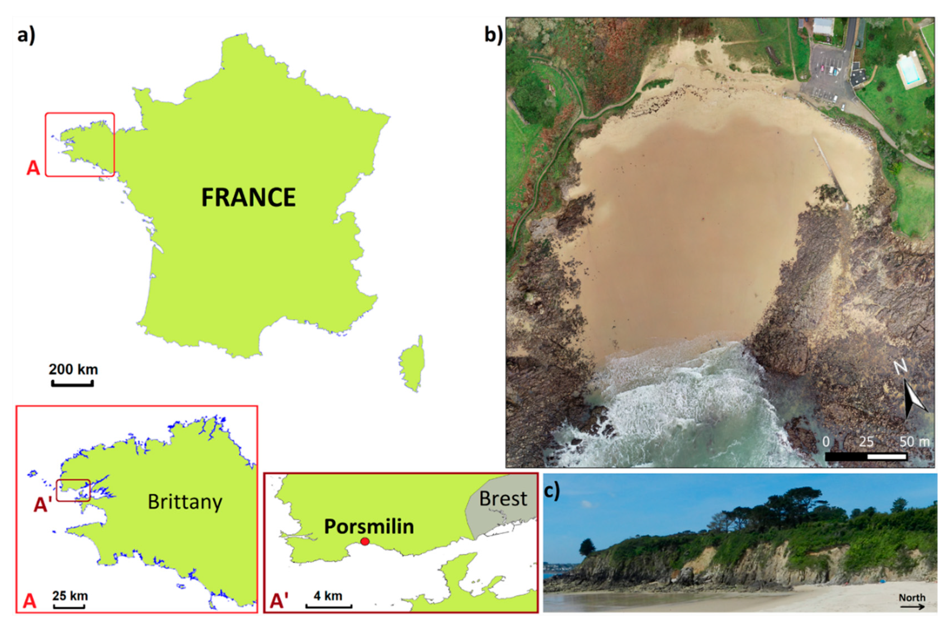
Porsmilin Beach (Figure 1) is located along a macrotidal coast (mean spring tidal range of 5.7 m), at the western end of Brittany (France). The Iroise Sea is a highly energetic environment, with annual and decadal significant wave heights of, respectively, 11.3 m and 14.5 m being measured in 110 m of water depth [26].

Porsmilin is a sandy embayed beach and, since 2014, is one of the sites followed in the framework of DYNALIT, the French National Observation Service dedicated to long-term observation of coastal dynamics (https://www.dynalit.fr/). To the north, the beach is backed by colmated brackish water marshes. To the east and west, it is flanked by orthogneiss cliffs of about 20 m high and bounded by headlands and bedrocks. Porsmilin beach has been regularly monitored since 2003 with monthly measurements of topographical cross-shore profiles, being completed by Digital Elevation Models (DEM) computed from UAV photographs since 2006 and from Terrestrial Laser Scanner (TLS) point clouds since 2009 [3,27].

Hydrodynamic processes and the morphodynamic response of the beach were evaluated during large-scale field campaigns in 2014 and 2016 [28,29]. Besides, the evolution of the western cliff was monitored using a multi-instrument and multi-parameter campaign during the winter of 2016/2017 [30]. The present methodological study also focuses on the western cliff face.

3. Materials and Methods

3.1. Measurement System

The underlying principle of the RTK GNSS-assisted terrestrial SfM photogrammetry method is to record camera positions with a centimeter accuracy. Accurately knowing these (X, Y, Z) coordinates simplifies the collinearity equations by removing unknowns, which do not need to be solved during bundle block adjustment while using GCPs. Using this approach, the camera orientation is not a priori measured, but estimated with tie points during bundle block adjustment.

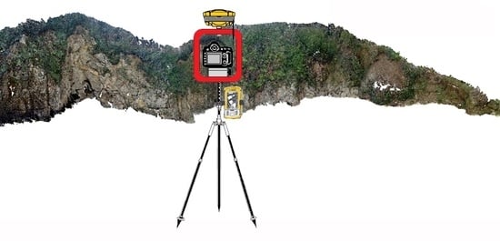
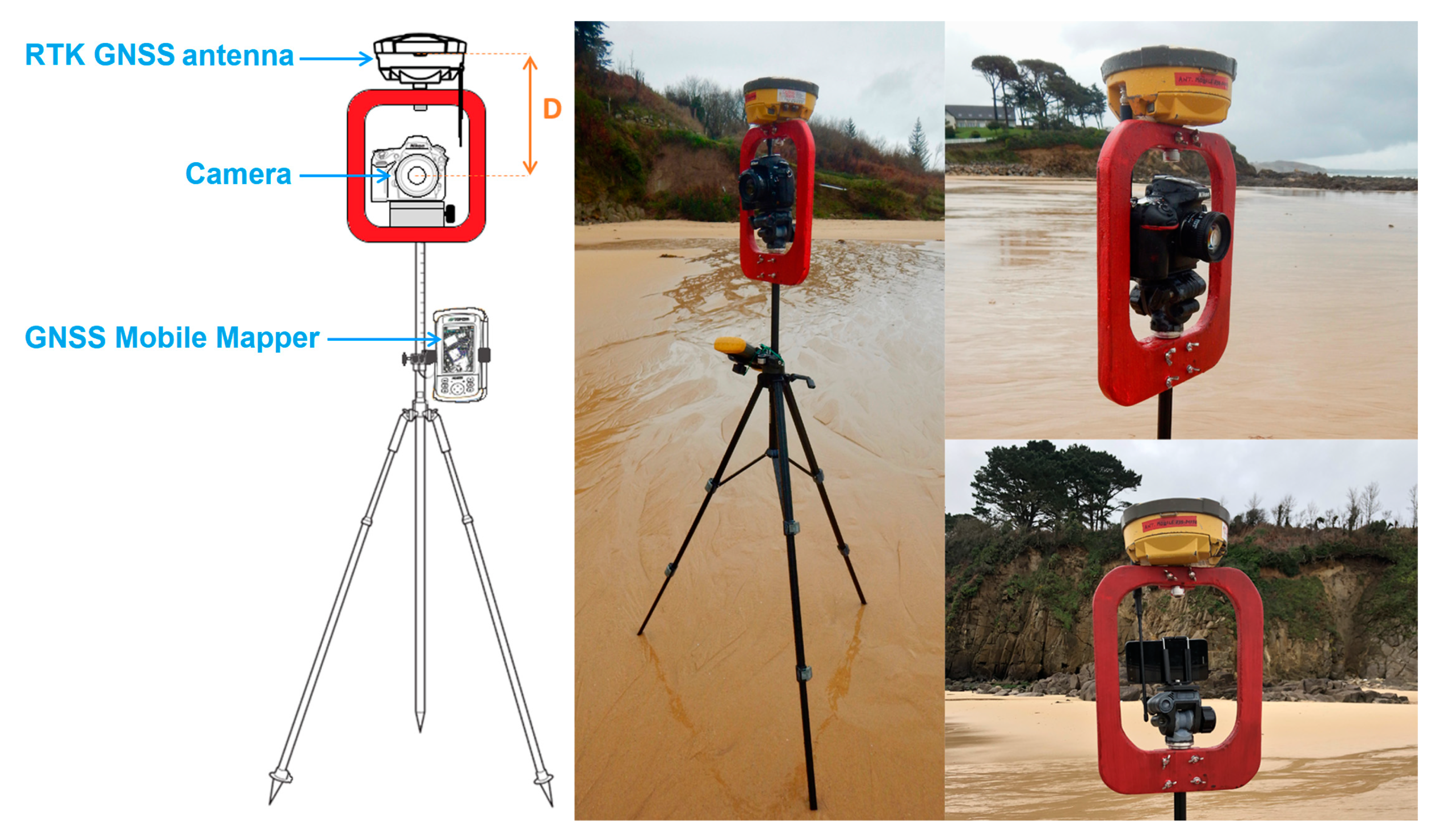
To record the camera position with sufficient accuracy, we developed a measurement system (Figure 2) that is composed of (i) a light tripod for photography, (ii) a custom-built wood frame, (iii) a camera (Reflex camera or Smartphone), and (iv) the mobile antenna and pad of a RTK GNSS. The wood frame is used to mechanically connect the mobile antenna of the RTK GNSS receiver and the camera.

For this study, we used a Topcon^® HiPer V GNSS receiver. The GNSS base station is set up on an existing geodetic marker located near the car park at the north-east of the study site (see Figure 1b). The same GNSS base was used for both the RTK GNSS-assisted terrestrial SfM photogrammetric survey and validation surveys.

We tested the method with a Nikon D800 Reflex camera (with a focal length of 20 mm) and with a Huawei Y5 (2016) Smartphone camera (with a focal length of 4 mm).

Table 1. Characteristics of the images taken by the Reflex camera and the Smartphone camera.

Camera Model	Reflex Camera—Nikon D800	Smartphone—Huawei Y5 2016
Focal Length	20 mm	4 mm
Image Size	3680 × 2456 pixels (9 Mpix)	3264 × 1840 pixels (6 Mpix)

summarizes the characteristics of the photographs taken with both sensors. All of the images were taken in landscape format, as it represents the easiest way to mount the camera on the tripod, also allowing for maximizing the spatial coverage for a given overlap.

The wood frame was designed so that the GNSS antenna and the camera center are vertically aligned. This configuration facilitates the pre-processing of data, since it limits the offset between the camera perspective center and the GNSS antenna phase center to a vertical component. Using this configuration, several images can be obtained from the same position by spinning the camera around this vertical axis, without moving the tripod. More particularly, having no horizontal offset between the camera and the GNSS antenna avoids having to determine the eccentricity vector for each shot and, hence, to determine the azimuth of the horizontal shift between the GNSS antenna phase center and the camera perspective center.

As the GNSS receiver is used to measure the camera position, not the ground topography, it is not necessary to measure or to keep constant the height of the camera above the ground. Indeed, as the distance (noted D) between the camera and the GNSS antenna is kept constant throughout all image acquisitions, this offset is directly subtracted from the position that is measured by the GNSS antenna (Equation (1)), providing accurate camera location.

$$\left(\begin{array}{c}{X}_{Cam}\\ Y_{Cam}\\ Z_{Cam}\end{array}\right)=\left(\begin{array}{c}{X}_{GNSS}\\ Y_{GNSS}\\ Z_{GNSS}\end{array}\right)-\left(\begin{array}{c}0\\ 0\\ D\end{array}\right)$$

(1)

with (X_Cam, Y_Cam, Z_Cam): position of the camera perspective center

(X_GNSS, Y_GNSS, Z_GNSS): position of the GNSS antenna phase center

D: vertical offset between the camera perspective center and the GNSS antenna phase center (D = 19.8 ± 0.1 cm for the Nikon D800 camera, respectively, D = 20.2 ± 0.1 cm for Huawei Y5 Smartphone). D was determined using a caliper, with millimeter precision.

The whole system is very easy to transport, weighing around 5.6 kg in the case of the Reflex camera (not including the GNSS base station). The autonomy of the system depends on the GNSS antenna battery, which is around 4 h for the GNSS that we used.

3.2. Survey Operational Mode

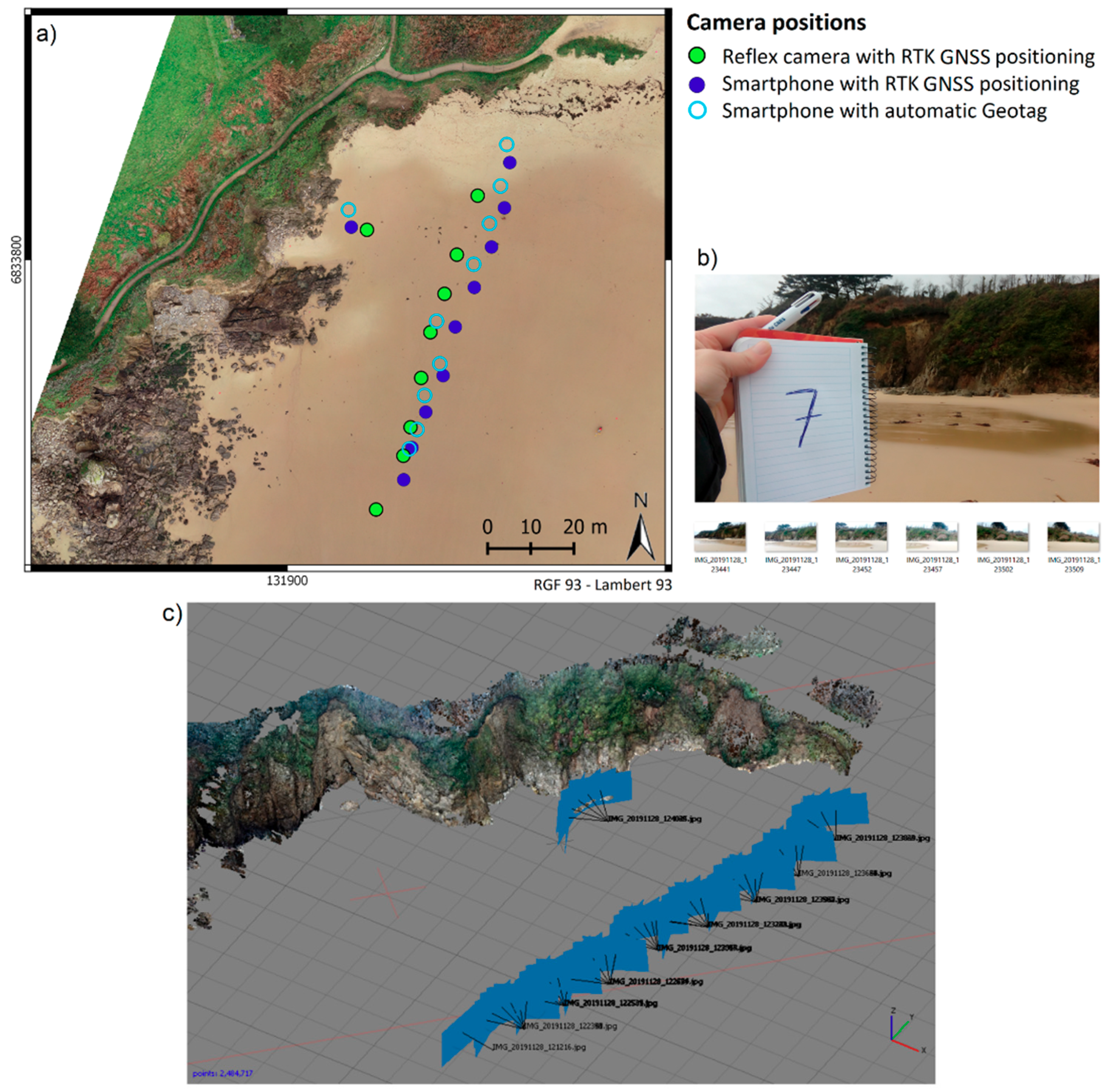
Photographs were taken at around 50 m from the cliff face (Figure 3a), which resulted in a mean pixel size of 1.60 cm/pixel with the Nikon Reflex camera and 1.93 cm/pixel with the Huawei Smartphone. Some extra photographs were taken from a closer position to limit occlusions, particularly as one section of the cliff is obstructed by a rocky outcrop. In general, not being too close to the cliff face is important for guaranteeing a good GNSS reception, a problem that is accentuated in cases where photogrammetry relies on GCPs attached to the cliff face.

For measuring the entire cliff face, the setup was moved to different camera stations. For each station, approximately five to ten photographs are collected according to a “fan-shaped capture” (i.e., spinning the camera around the vertical axis [9]) and the station position is measured by RTK GNSS using a 30-s average. The system is then moved to the next station, without being dismantled. For each new position, a first photograph is taken in order to indicate the number of the station and make associating the correct position to each photograph easier (cf. Section 3.3 and Figure 3b). Using this approach optimizes the image overlap, so that each point is captured by more than nine photographs.

For our tests, two different camera models were used (Table 1). In the case of the Huawei Y5 Smartphone camera, which is equipped with an internal GNSS, we also tested the possibility of using the image geotags provided by the smartphone.

Table 2. Image acquisition carried out with the Nikon D800 reflex camera (test 1) and with the Huawei Y5 Smartphone (test 2).

Camera Model	Reflex Camera—Nikon D800	Smartphone—Huawei Y5 2016
Number of camera positions	9	10
Mean distance between successive camera positions	≈10 m	≈10 m
Height of the camera above the ground	≈1.5 m	≈1.5 m
Mean distance to the cliff face	≈45–50 m	≈50 m
Mean pixel size	1.60 cm/pix	1.93 cm/pix
Number of images	76	63

summarizes the main characteristics for each test. The total number of collected photographs is larger for the Reflex camera than for the Smartphone camera. This is due to the image format (3/2 for the Reflex camera versus 16/9 for the Smartphone camera) paired with a shorter focal length for the Smartphone camera, meaning that the desired surface coverage with a sufficient image overlap is achieved with fewer photographs with the Smartphone. The duration of a survey (including assembly of the system) was about 30 min.

3.3. Data Processing

Geolocated photographs were processed using SfM photogrammetry integrated in the popular software Agisoft PhotoScan^® Pro v1.2.3 (Figure 3c). The first step before data processing consists in creating and formatting a camera position file compatible with PhotoScan^®. This file is composed of four columns: a label (corresponding to the name of each photograph) and the easting, northing, and altitude coordinates of the camera measured by the RTK GNSS. The altitude provided by the RTK GNSS must be corrected from the vertical offset D (as explained in Section 3.1). As several photos were taken from the same position, they share the same coordinates.

All datasets are processed using the same parameters in the processing software to avoid biases in the comparison between Reflex and smartphone camera datasets (cf. below). The main steps of the image matching and stereorestitution process are:

-

Image orientation by bundle adjustment (detection and matching of homologous keypoints in overlapping photographs in order to compute the external parameters for each camera). The accuracy is set to “high”, which means that the software works with the photos of the original size. Key point limit and tiepoint limit are set to their default values.

-

Refinement of camera calibration parameters (internal parameters) using the camera positions (parametrized with an accuracy of 5 cm in the Reference pane in PhotoScan^®, i.e., the RTK GNSS-measured positions are taken as initial values and their variations during bundle block adjustment process are constrained in a radius of 5 cm).

-

Dense image matching to produce a dense point cloud using the estimated external and internal camera parameters. For this step, the accuracy parameter is set to “high” to obtain more detailed and accurate geometry and the depth filtering mode is set to “aggressive”.

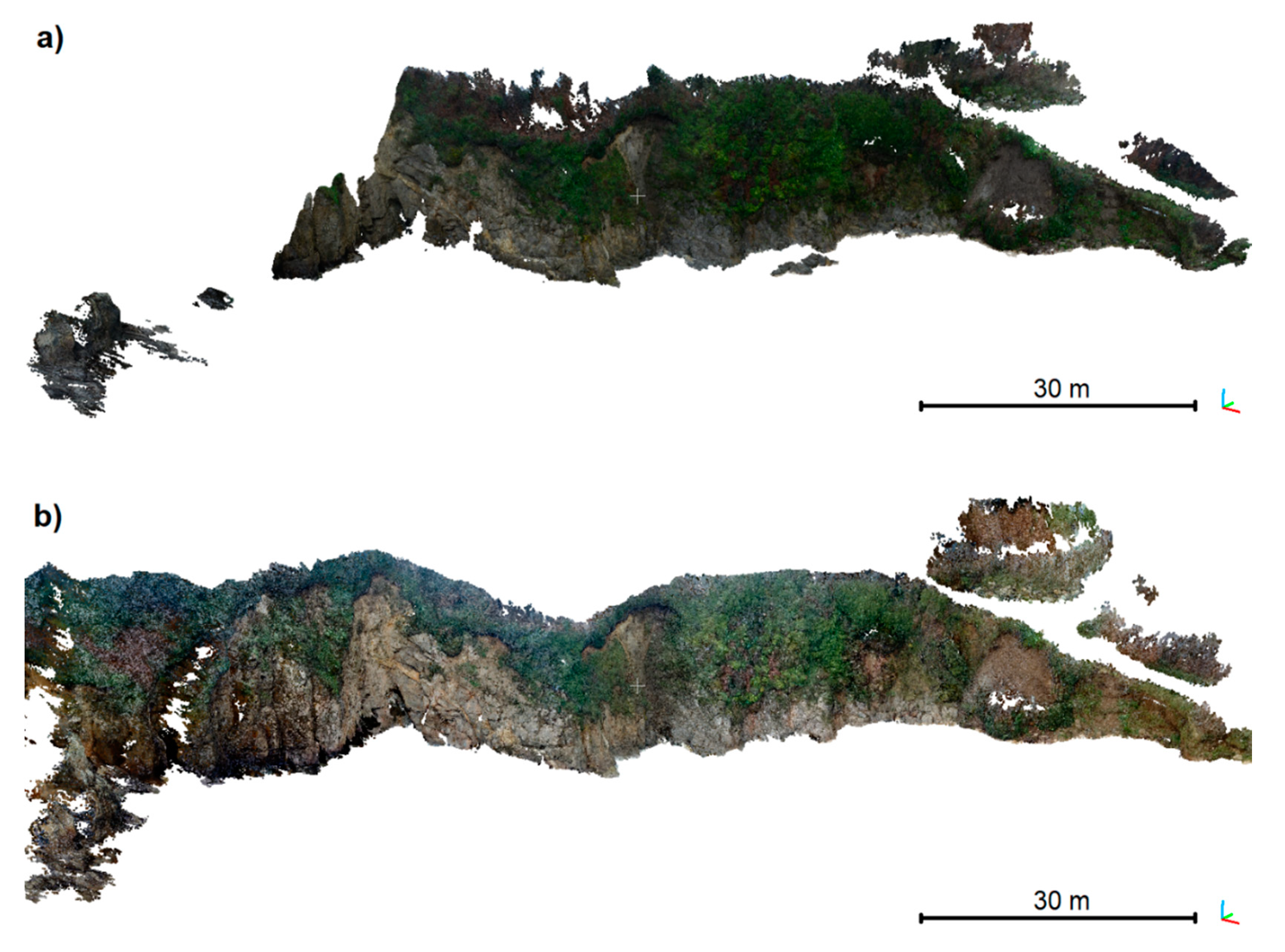
The colored dense point cloud is exported as the final result (Figure 4). Indeed, georeferenced DEMs and orthophotographs are not as interesting, as the study focuses on sub-vertical objects (cliffs).

The dense point cloud obtained with the Huawei Smartphone covers a larger area than the Nikon point cloud, including stable sections of the cliff that are not concerned by the monitoring, as shown in Figure 4. The reason is image size, which, as mentioned before, is more panoramic for the smartphone and, therefore, provides a higher overlap on external parts of the survey area.

Two processing methods are performed for the survey with the Smartphone camera (Test 2): one with the camera position file created from positions measured by RTK GNSS (Test 2a), another using the geotag of the photographs and so the position measured by the Smartphone internal GNSS (Test 2b). For Test 2a, the camera position accuracy was set to 5 cm, whereas it was set to 5 m for Test 2b. Comparing the camera positions measured by the RTK GNSS and by the Smartphone’s internal GNSS (single frequency GNSS) provided a Root Mean Square Error (RMSE) of 3.44 m.

3.4. Validation Data

Porsmilin beach is one of the field sites regularly monitored in the framework of the long-term coastal observatory DYNALIT. For this campaign, a TLS survey was performed simultaneously to the GNSS-assisted terrestrial photogrammetry surveys. This TLS survey involved two scans from two distinct scan positions performed with a Riegl^® VZ-400, with each scan covering 360° horizontally and 100° (from 30° to 130°) vertically with an angular resolution of 0.04° in both directions.

Associated to the TLS survey, the position of reflective targets was measured via RTK GNSS. The targets are reflective cylinders (10 cm in diameter and 10 cm in height) distributed around the TLS standpoint before the survey. The processing of the TLS data was performed using the RiScanPRO^® software suite (provided by Riegl^®) and CloudCompare^® [31], a 3D point cloud freeware processing software. It comprised three main steps:

• Georeferencing and individual clouds assembly. An indirect georeferencing was performed using the reflective targets (e.g., [32]).
• Manual point cloud filtering to remove artefacts and undesirable data (people on the beach, data outside of the study area, etc.)
• Point cloud interpolation onto a mesh, based on a Triangular Irregular Network (TIN).

TLS datasets are often used as reference, because, contrary to SfM photogrammetry, measurement errors that are related to the accuracy of the laser are constant across the point cloud, with errors that are inherent to georeferencing being transmitted to the whole cloud [8]. Under similar survey conditions, TLS accuracy on recurrent cliff face surveys was estimated to be around 3 cm [8]. Here, the cliff face that was measured by TLS was used as large-scale validation data to assess the accuracy (represented by mean error) and precision (represented by standard deviation of error) of the SfM photogrammetric point clouds. This approach ensures a global assessment of the error, while taking into account the error spatial variability due to reconstruction artefacts or environmental parameters. This assessment was performed using the “cloud-to-mesh distance” tool, computing nearest-neighbor distances in CloudCompare^®. Using a mesh for the TLS dataset avoids computational artefacts in quality assessment, which might be introduced due to a heterogeneous point cloud density.

Nevertheless, the TLS point cloud is not error-free, and having a lower spatial resolution than SfM photogrammetric reconstructions, it is not fully relevant at small scale. Therefore, the consistency at small scale of the SfM reconstructions was also assessed by inter-comparing the SfM dense point clouds that were obtained using the Nikon Reflex camera and the Huawei Y5 Smartphone camera, respectively.

4. Results

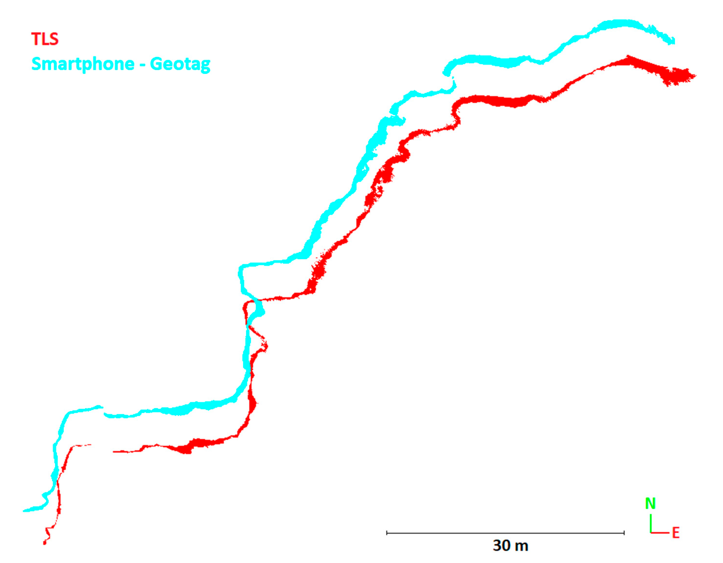
For the tests that were conducted using the Huawei smartphone, we mentioned previously a RMSE of 3.44 m between the camera positions measured by the RTK GNSS and by the Smartphone’s internal GNSS (cf. Section 3.3). This deviation can be explained by the low precision of the internal GNSS module (~5 m) in comparison to RTK GNSS (~cm). Unsurprisingly, this has an impact on the SfM reconstruction performed while using the Geotag of the photographs (Test 2b). Figure 5 presents a top view comparison of the cliff front position obtained with the TLS and by SfM reconstruction using the Geotagged photographs. The mean error comparing the Geotagged SfM point cloud to the TLS mesh is 2.13 m with a standard deviation of 1.22 m. However, for estimating this error, CloudCompare^® measures the normal distance between a point and the closest facet on the TLS mesh, even if it does not correspond to the same portion of the cliff. The difference between the Geotagged SfM point cloud and the TLS point cloud was assessed by performing an automatic registration in CloudCompare^®, which is based on an Iterative Closest Point (ICP) algorithm. The difference is mainly a translation (with Tx = 0.55 m, Ty = −4.46 m and Tz = −0.36 m), but, correcting this translation, the residual average error between the Geotagged SfM point cloud and the TLS mesh is still of 0.10 m with a standard deviation of 0.36 m, implying that other sources of errors (e.g., scale, deformation) are also present. As the geotagged Smartphone dataset is not exploitable without having to recur to a reference dataset for correction, this configuration will not be used again for the rest of the study.

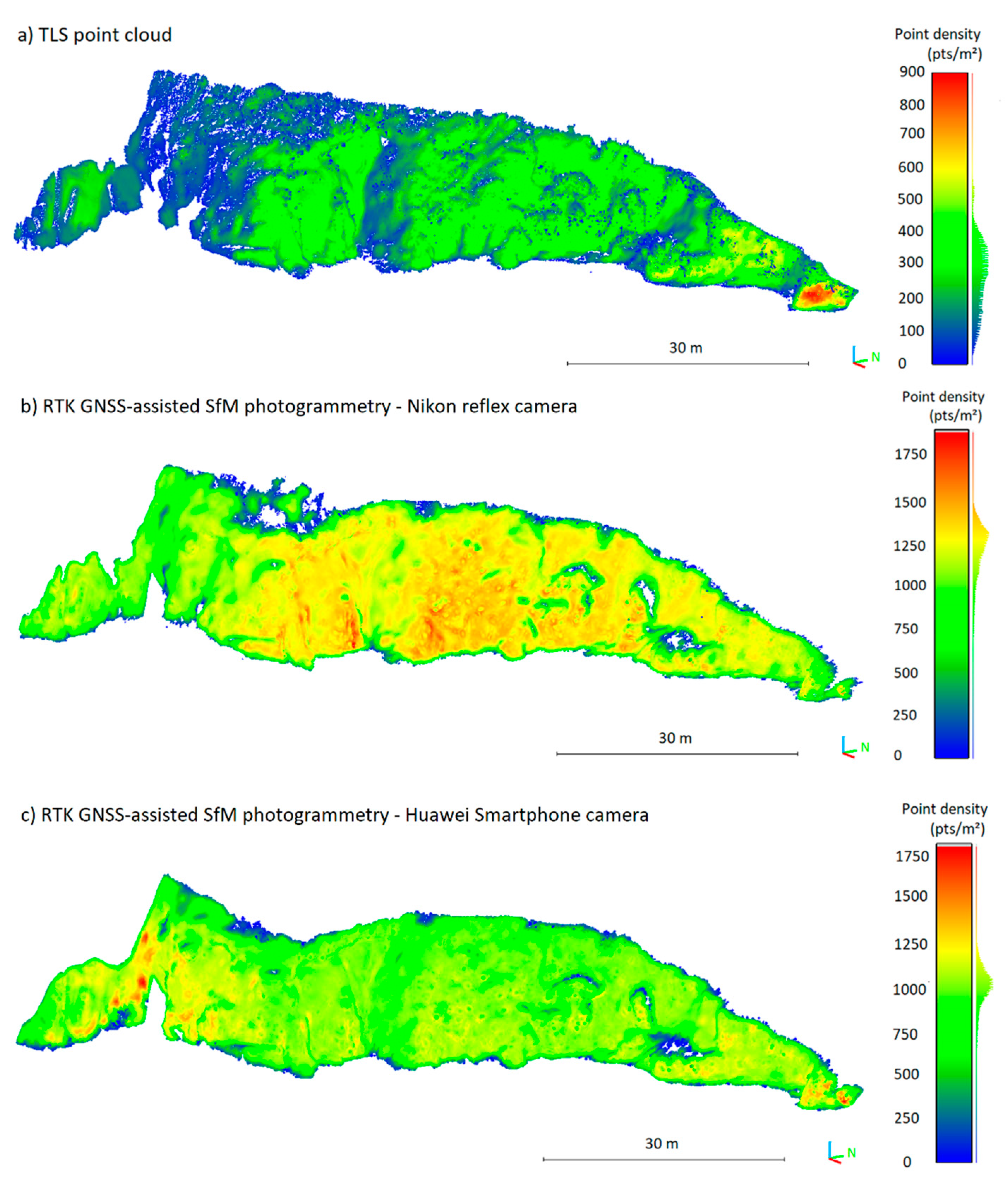
In the following, the SfM reconstructions obtained with the RTK GNSS-assisted system combined with Nikon D800 Reflex photographs (Test 1) and Huawei Smartphone photographs (Test 2a) are compared with the TLS point cloud and the resulting TLS mesh. In terms of point density, the TLS point cloud averages 84.6 points/m² (

Table 3. Comparison of point density for TLS and SfM reconstructions.

TLS Point Cloud Density	84.6 pts/m2
	Reflex Camera—Nikon D800	Smartphone—Huawei Y5 2016
Tiepoint density	0.80 pts/m2	1.99 pts/m2
Dense point cloud density	476.9 pts/m2	388.3 pts/m2

), with the actual point density varying depending on the TLS scan position and the angle of incidence of the laser ray with the cliff face (Figure 6a). The dense point clouds obtained by RTK-GNSS assisted SfM photogrammetry are four to six times denser than the TLS point cloud, with an average density of 476.9 points/m² for the Nikon D800 Reflex camera and 388.3 points/m² for the Huawei Y5 Smartphone camera (Table 3). Furthermore, the point density obtained with the RTK GNSS-assisted SfM photogrammetry is more homogeneous than for the TLS acquisition (Figure 6).

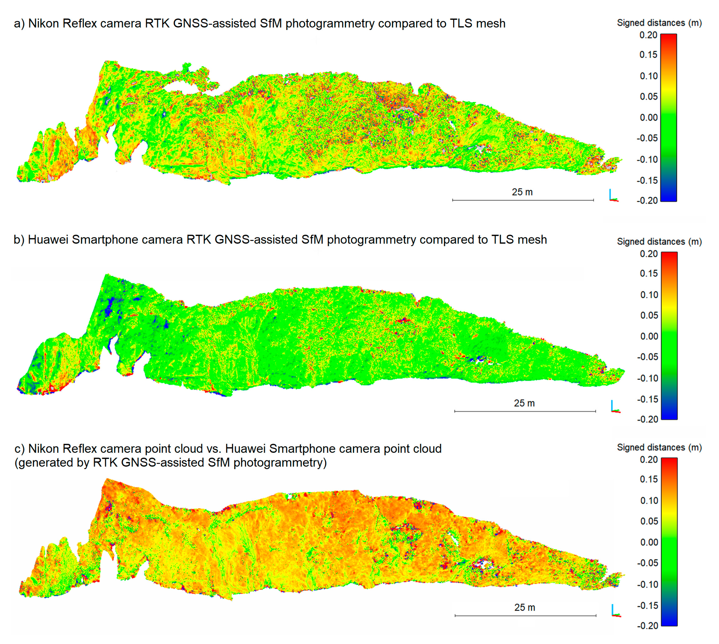
Comparisons of SfM point clouds with the TLS mesh (

Table 4. Cloud-to-mesh distances between the TLS mesh (used as reference) and RTK-GNSS assisted SfM dense point clouds.

Comparison to TLS Mesh	Mean Error (m)	Standard Deviation (m)
Reflex camera—Nikon D800	0.003	0.047
Smartphone—Huawei Y5 2016	0.002	0.038
Comparison Reflex camera vs. Smartphone	0.005	0.061

) show a mean error of 0.3 cm and standard deviation of 4.7 cm for the Nikon D800 Reflex camera (Figure 7a) and, respectively, a mean error of 0.2 cm and standard deviation of 3.8 cm when using the Huawei Y5 Smartphone camera (Figure 7b). Comparing the SfM point cloud obtained with the Nikon D800 Reflex camera to the one obtained with the Huawei Y5 Smartphone camera (Figure 7c), the mean error is of 0.5 cm and the standard deviation of 6.1 cm. Figure 7c suggests that the Nikon camera point cloud is often ahead of the Smartphone point cloud, although this observation is not verified when looking at the mean error (Table 4). We think that the mean error calculation might be impacted by large negative deviations between the two point clouds, which could, in effect, balance out the more frequent but smaller positive differences. For both SfM point clouds, larger differences are situated on the fringes of the measured area and may be due to slight differences in spatial data coverage between the SfM point clouds and the TLS mesh. 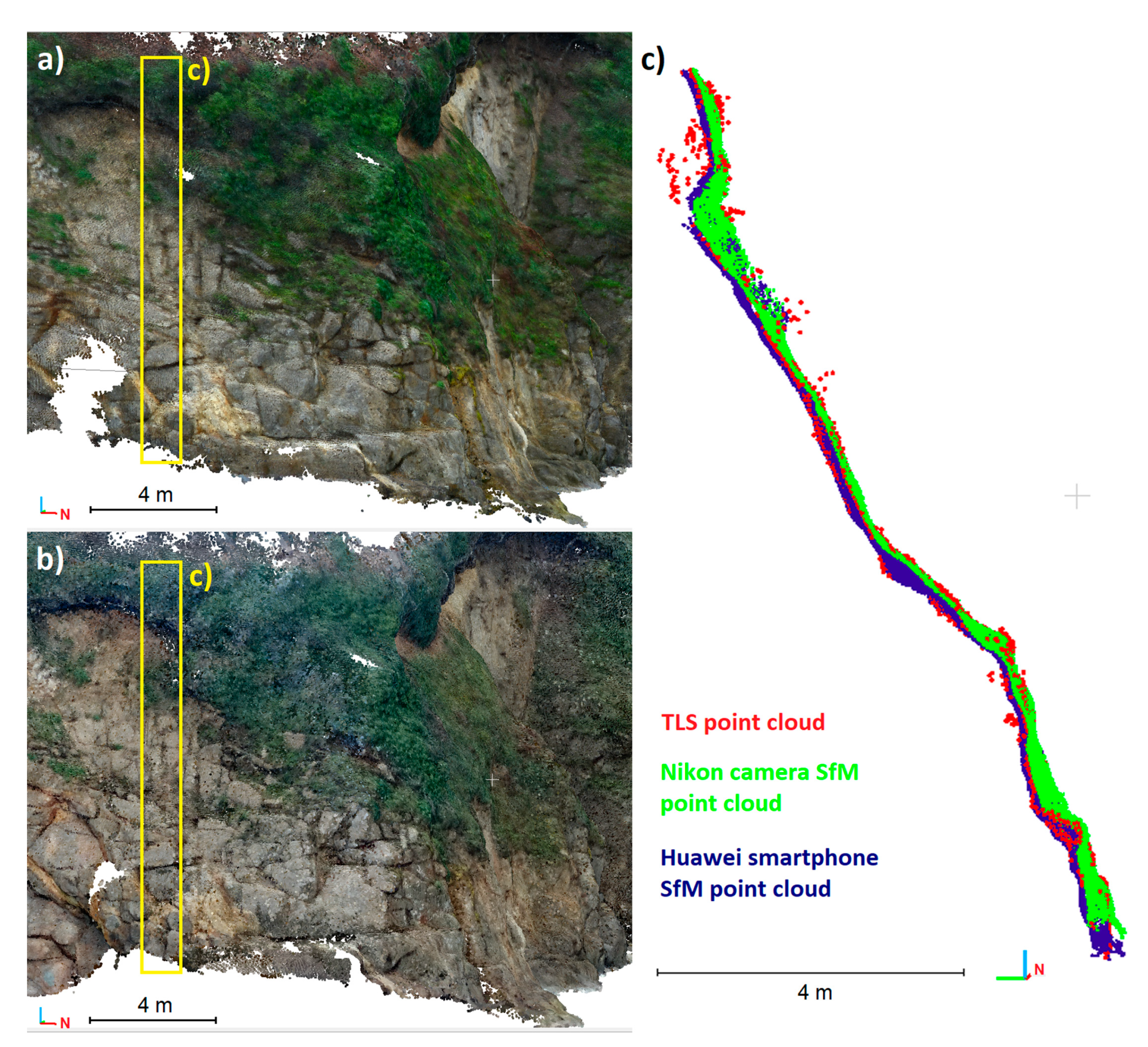For the Reflex camera SfM point cloud, most of the difference corresponds to vegetated areas (Figure 7a), which are challenging to measure using either SfM photogrammetry or TLS. When considering the order of magnitude of the differences, we have indeed to keep in mind that the TLS mesh can also be affected by measurement errors or interpolation errors due to lower point density during mesh creation. Furthermore, it is interesting to note that the errors we measured during this study are lower than the accuracy expected for RTK-GNSS measurements (around 2 to 4 cm). Paradoxically, when visually comparing both SfM point clouds (Figure 8a,b), we can notice that the rendering of the Smartphone point cloud seems noisier than the rendering of the Reflex camera point cloud. Nevertheless, this difference in aspect is, in all likelihood, due to contrast, luminosity, and radiometric differences in the images, independently of the geometric reconstruction. A vertical topographical profile (Figure 8c) confirms that the SfM point clouds are very coherent with each other (with the Nikon camera point cloud slightly ahead of the Smartphone one) and that they can differ from the TLS point cloud over vegetated areas.

5. Discussion

Traditionally, in many aerial and terrestrial photogrammetric applications, using a good network of GCPs has been shown to be an important prerequisite to guarantee the quality of the SfM reconstruction (e.g., [14,16]). In the framework of a coastal observatory, such as DYNALIT, using recurrent surveys for monitoring beach and cliff morphodynamics, measurement quality is critical for producing reliable estimates of sediment budgets and, hence, for assessing the tendency to erosion for a particular section of the coast. Yet, the necessity to adopt a protocol as simple, quick, and standardized as possible to limit the operator dependency of the results is perhaps as much important when considering repeated surveys.

When compared to field applications of photogrammetry using a GNSS for independently measuring GCPs distributed on the ground, our approach replaces the GCPs by a solid frame connecting the camera and the GNSS antenna. Not requiring GCPs, this RTK GNSS-assisted method enables saving time in the field, since it is notorious that setting up a good network of GCPs can be time consuming, and it also reduces the bulk of the equipment needed on site. Furthermore, it is sometimes impracticable to use GCPs in some parts of the study site because of inaccessibility or the impossibility of GNSS measurement due to obstructions (e.g., cliff, trees). The GNSS-assisted method also enables avoiding the time-consuming step of GCP identification, whereby GCPs must be identified from photographs during the photogrammetric processing. In terms of the quality of photogrammetric results, the independency to GCP distribution limits the risks of geometrical distortions in the SfM reconstruction induced by poor GCP distribution [18].

In the present work, we achieved centimeter-scale accuracy without the need for a-priori camera calibration. The latter is important for process simplification and for the larger uptake of the technique, including outside academic circles. Furthermore, as the GNSS antenna and the camera are aligned on the same vertical axis, our system enables taking several pictures from the same position by spinning the camera. This fan-shaped acquisition enhances the image overlap, which is favorable for bundle adjustment. Furthermore, we obtained highly satisfying results, with mean errors lower than a centimeter, whereas previous studies achieved absolute accuracies on check points ranging from 4 to 7 cm [25]. That can be due to the fact that previous work concentrated on applications in an urban area, where the GNSS signal is not optimal. Moreover, we simplified the method by aligning our RTK GNSS antenna and our camera along the same vertical axis, reducing the number of additional measurements.

Among other advantages, the system that we present is simple to implement, low cost (as the frame can be custom-built out of simple wood), versatile (it is compatible with any GNSS antenna and virtually any type of cameras from bulky reflex to Smartphone cameras), and it offers long autonomy, enabling long survey sessions, only being limited by the GNSS battery autonomy (in our case, around 4 h for a battery). The operator time during processing is drastically reduced, since no GCP pointing on the photographs is needed. Throughout the tests that we performed, the method provided very satisfying results, both in terms of point density and accuracy, even near a cliff face, which must rate as a difficult measurement site because of the obstructed view of the satellite constellation, of the complex geometry of the face with concavities, fissures, and vegetated areas. This approach is very promising for cliff face reconstruction, since it is very difficult to install GCPs in this environment and given that a terrestrial point of view is favorable to capture its complexity. In addition, we can infer that, as long as a GNSS signal is available, the method can be easily applied to other domains that are interested in terrestrial photogrammetry, including, but not limited to, urbanism, archaeology, and structural geology [33,34].

Going forward, a possible improvement would be to replace the Topcon RTK GNSS antenna with a low cost GNSS positioning system to make the approach even more cost-effective and easily transposable to participatory science programs or citizen observatories. We have shown that using the Smartphone Geotag of the photographs is not sufficiently accurate. Furthermore, the accuracy of the Geotagging varies significantly (several meters) from one Smartphone model to another, from one day to another, and from a type of environment to another. For example, for this study, we obtained a RMSE of 3.44 m with the Huawei Y5 Smartphone. A month later, with an iPhone 8 Smartphone, we obtained a RMSE of 5.11 m. In the literature, we can find Smartphone positioning RMSE ranging from 4.51 to 11.45 m under forest canopies [35] or from 7 to 13 m in an urban environment [36]. Using an open RTK GNSS network, for instance, such as that provided by Centipède RTK (https://centipede.fr/), which provides low cost systems for centimeter-scale accuracy positioning, could be a promising avenue for expanding the use of our RTK GNSS-assisted terrestrial SfM photogrammetry method.

6. Conclusions

The proposed method of RTK GNSS-assisted terrestrial SfM photogrammetry and the associated acquisition system enable low-cost and high-quality photogrammetric surveys without requiring GCPs. By comparison to a synchronous TLS survey, a mean error of 0.3 cm (standard deviation of 4.7 cm) was obtained with a Nikon D800 Reflex camera and, respectively, a mean error of 0.2 cm (standard deviation of 3.8 cm) with a Huawei Y5 Smartphone camera. Avoiding the use of GCPs saves considerable time during the field survey as well as during data processing. This method will be particularly interesting when simplicity, portability, and autonomy are desirable. In the future, using an open RTK GNSS network would help to make this approach transposable to participatory science programs and citizen observatories.