Reservoir Induced Deformation Analysis for Several Filling and Operational Scenarios at the Grand Ethiopian Renaissance Dam Impoundment


Department of Geography, University of California, Los Angeles, 1255 Bunche Hall, Box 951524, Los Angeles, CA 90095, USA
*
Author to whom correspondence should be addressed.
Remote Sens. 2020, 12(11), 1886; https://doi.org/10.3390/rs12111886
Submission received: 2 May 2020
/
Revised: 6 June 2020
/
Accepted: 9 June 2020
/
Published: 10 June 2020
(This article belongs to the Special Issue Earth Observations for Land Subsidence Identification, Monitoring and Their Contribute to Modeling)
Abstract
:Addressing seasonal water uncertainties and increased power generation demand has sparked a global rise in large-scale hydropower projects. To this end, the Blue Nile impoundment behind the Grand Ethiopian Renaissance Dam (GERD) will encompass an areal extent of ~1763.3 km2 and hold ~67.37 Gt (km3) of water with maximum seasonal load changes of ~27.93 (41% of total)—~36.46 Gt (54% of total) during projected operational scenarios. Five different digital surface models (DSMs) are compared to spatially overlapping spaceborne altimeter products and hydrologic loads for the GERD are derived from the DSM with the least absolute elevation difference. The elastic responses to several filling and operational strategies for the GERD are modeled using a spherically symmetric, non-rotating, elastic, and isotropic (SNREI) Earth model. The maximum vertical and horizontal flexural responses from the full GERD impoundment are estimated to be 11.99 and 1.99 cm, regardless of the full impoundment period length. The vertical and horizontal displacements from the highest amplitude seasonal reservoir operational scenarios are 38–55% and 34–48% of the full deformation, respectively. The timing and rate of reservoir inflow and outflow affects the hydrologic load density on the Earth’s surface, and, as such, affects not only the total elastic response but also the distance that the deformation extends from the reservoir’s body. The magnitudes of the hydrologic-induced deformation are directly related to the size and timing of reservoir fluxes, and an increased knowledge of the extent and magnitude of this deformation provides meaningful information to stakeholders to better understand the effects from many different impoundment and operational strategies.
1. Introduction
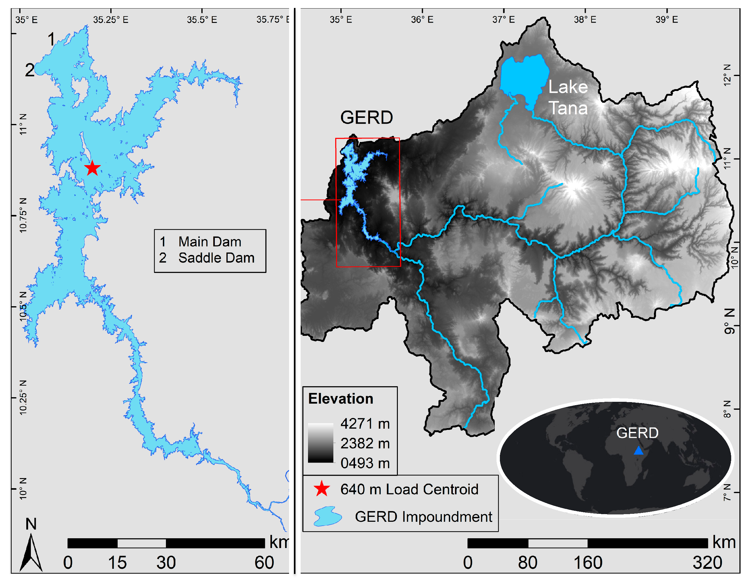
The Grand Ethiopian Renaissance Dam (GERD) on the Blue Nile is located in Ethiopia about 15 km upstream (east) of the Sudanese border and is set to be complete in the next several years [1,2]. The initial GERD site itself was one of four identified during a survey in the 1960s by the United States Bureau of Reclamation [3]. The dam is located around 11.215° N, 35.092° E (Figure 1) and sits in the Upper Blue Nile Basin, a large watershed with an areal extent of ~175,000 km2. The notable Ethiopian Highlands drain through the basin and into the Blue Nile, and subsequently to the GERD impoundment. Construction on the dam began in the spring of 2011, and when completed, it will be the largest dam in Africa. The main roller compacted concrete gravity dam is 150 m tall and 1800 m long and will work in unison with an adjacent rock-filled saddle dam that is ~50 m tall and 5 km long in order to increase the water level of the impoundment to approximately 640 m above mean sea level [4,5,6]. The entire Blue Nile River Basin contributes around 58–62% of the total water supply to downstream Nile River flows [7]. Blue Nile flow data at the Sudanese/Ethiopian border from the National Meteorological Agency of Ethiopia have a historical (1967–1972; 1999–2003) annual mean of around 50 Gt, where the vast majority (~80%) of this flow occurs in the months of July through October [2,8,9].
The impoundment of the Blue Nile at the GERD site will have a multitude of different impacts. The annual discharge curve will be severely altered due to the GERD construction and the subsequent large volume of the impoundment. The large capacity of the GERD impoundment allows for a near-equal discharge for each month of the year, allowing for a reduction in both high and low Blue Nile flow events [7]. To this end, there will likely be fewer flood and drought events and the region’s hydrologic uncertainty will be reduced. The GERD is not the first dam on the Blue Nile or the Nile. However, the upstream location coupled with the size of the reservoir will affect the already completed downstream hydrologic engineering projects. For example, three downstream dams (Rosaries, Sennar, and Aswan High) will need to adjust their release operations in order to maintain Sudanese agricultural water supplies [10]. Downstream hydrologic power generation could possibly be affected by the filling and operation of the GERD impoundment. The potential reduction in power generation will be related to the filling and operational scenarios that the GERD water managers decide upon [6,10,11].
Groundwater levels are also likely to be impacted by the GERD impoundment and subsequent reservoir operations. To this end, reservoirs can provide seepage into the subsurficial rock and connected aquifer systems. This diffusion of water into the underlying rock is capable of increasing pore pressure and reducing frictional stresses. Further, impoundment and operational strategies of large dams (e.g., Three Gorges) have been shown to directly alter groundwater levels for hydraulically connected aquifer systems [12,13]. These connections are capable of decreasing slope stability and can trigger slope failure events as caused by the changes in hydrostatic pressure due to the varying levels in the groundwater and the hydraulically connected reservoir levels [14,15,16,17].
Other impacts from the GERD impoundment are related to the large hydrologic loading forces applied to the reservoir-adjacent lithosphere. Drastic changes in surface loads brought on by large hydro-engineering projects can have far reaching implications for increased stress and strain on surrounding fault systems and subsequent seismicity [18,19,20,21,22,23]. The initial GERD impoundment and subsequent reservoir creation along with seasonal fluxes in water levels due to operational phases cause large changes in both the areal extent and volumetric content of the reservoir. These marked variations in hydrologic loads can impart large forces on the surface of the Earth and are capable of deforming the lithosphere. For example, numerous studies have shown that in situ and remotely sensed products (e.g., GNSS, InSAR, GRACE, etc.) are capable of quantifying the flexural response from changes in hydrologic loads (snow, reservoirs, seasonal precipitation, drought, regional climatic changes, lakes, etc.) [24,25,26,27,28,29,30,31]. The size of the GERD project allows for a large influx of water into the upstream reservoir area during the filling stages as well as during normal seasonal operation. These loads are highly dependent on the chosen filling and operational strategies. The amplitude and extent of the flexural response is mostly dependent on the underlying rheology as well as the timing and amount of the hydrologic forcing. Both the early filling stages and the subsequent operational scenarios play important roles in the application of hydrologic load induced lithospheric deformation for an impoundment of this size.
This study seeks to provide a first look at the modeled vertical (subsidence and uplift) and horizontal displacement brought on by the initial GERD impoundment along with reservoir operations from several predicted seasonal release plans. This work was undertaken in order to glean a better understanding of the amplitude and spatiotemporal dynamics of the load-induced flexural response at and around the GERD study site. In order to accomplish this task, we seek to answer the following questions: (1) What are the areal extents, reservoir volumes, and hydrologic loads from potential scenarios of long-term reservoir operation and multi-year reservoir filling schedules? (2) What are the modeled elastic flexural responses as caused by hydrologic loading variations from long-term reservoir operations and multi-year reservoir filling schedules at the GERD? We utilize digital surface models (DSMs) and hydrologic inputs from several filling and operational scenarios to answer (1), and we use those results along with a localized Earth model to compute the elastic displacements for each of the scenarios in order to answer (2).
2. Data and Methods
2.1. Reservoir Extents, Volumes, and Loads
Traditional remote sensing techniques to delineate water/reservoir extents (e.g., multispectral and/or radar satellite platforms) cannot be employed in this situation as the final GERD impoundment process has not yet begun. Instead, this study utilizes a DSM-based technique to determine areal extents and loads for varying reservoir levels behind the GERD. Several remotely sensed DSMs were examined in order to more precisely derive the areal extent, reservoir volume, and hydrologic load for every 1 m increment of the GERD impoundment. We inspected five different well-known DSMs that encompass the entirety of our study area, and selected the most accurate surface model based on a comparison of overlapping data from the Geoscience Laser Altimeter System (GLAS) instrument onboard the Ice, Cloud, and land Elevation Satellite (ICESat) platform. More specifically, we tested three DSMs generated from Shuttle Radar Topography Mission (SRTM) data (one arcsecond void filled, three arcsecond void filled, three arcsecond not void filled), one derived from Advanced Land Observing Satellite (ALOS) data, and another from Advanced Spaceborne Thermal Emission and Reflection Radiometer (ASTER) data [32,33,34]. All five surface models were mosaicked to encompass the entirety of the study area (all DSM grids encompassing the minimum bounding box around the extent of the full GERD impoundment) and were then projected to UTM Zone 36N (EPSG: 32636) using the WGS84 ellipsoid.
We acquired all GLAH14 (Land Elevation; Version 34) GLAS tracks from the National Snow and Ice Data Center (NSIDC) that overlap the five different mosaicked DSMs mentioned above [35]. GLAH14 elevation products are provided in ellipsoidal heights referenced to the Topex/Poseidon (TP) ellipsoid. As such, the GLAH14 data were converted to orthometric height above the WGS84 reference ellipsoid by subtracting the corresponding EGM96 geoid from the TP ellipsoidal heights and then subtracting 0.7 m. The WGS84 coordinates were projected to UTM Zone 36N (EPSG: 32636) in order to be directly comparable to the five DSMs investigated in this study. Lastly, the elevation values were filtered using the “sat_corr_flg” (saturation correction) and “FRir_qa_flg” (cloud presence) flags to only keep unsaturated elevation GLAS points and to further filter the GLAS data to only include cloud-free pulses, respectively. We compared overlapping GLAS pulses to the nearest DSM cell value for each of the five elevation models mentioned above in order to determine the appropriate DSM used to derive the most reliable hydrologic load inputs for our deformation models (as discussed in Section 2.2). We calculated the mean absolute difference and standard deviation for all quality GLAS pulses from the nearest cell for each of the five DSMs at five different slope bins of less than or equal to 1°, 3°, 5°, 10°, and 90° (i.e., all data). Mean absolute differences were derived for several slope bins in order to better determine the most accurate DSM to select for further processing. Areas with larger slopes can cause increased ground elevation values within the ~70 m GLAS footprint. These increased elevation ranges can decrease the accuracy of the returned GLAS elevation value as the elevation variation affects the GLAS laser return time and power, and subsequently negatively affects the final ellipsoidal height given by the GLAH14 product. We utilize Table 1 to show the GLAS comparisons for each of the slope bins for the five DSMs investigated. We note that the AW3D30 DSM has a lower mean absolute difference for each of the five different slope bins as compared with every other DSM we investigated. Similarly, the standard deviations are almost always lower for the AW3D30 DSM as compared with the other four surface models. The overall lower mean absolute differences and associated standard deviations for the AW3D30 DSM are evident in this table and highlight why we have selected this surface model for our hydrologic calculations. For comparison, we display the meter-by-meter areal extent and volumetric water loads for each of the five DSMs mentioned above in Table S1. We note increases of ~7% and ~19% in areal extent and volumetric water load for the least accurate DSM investigated as compared to the results from the AW3D30 DSM that we have utilized for our final reservoir calculations. We describe the ALOS-based DSM in the following paragraph.
The ALOS DSM was acquired from the Japan Aerospace Exploration Agency (JAXA) and is part of the ALOS World 3D-30m (AW3D30) project. The surface model has a cell spacing of 1 arcsecond (~30 m) and a vertical height accuracy of 4.4 m (RMSE). The AW3D30 product was up-sampled from the AW3D version (~5 m cell size) using a simple average of the 49 (7 × 7) underlying AW3D cells, and consists of 16-bit signed integer values [36]. We mosaicked three AW3D30 grids (N009E035, N010E035, N011E035) over the study region and manually adjusted the cells where the GERD infrastructure (main dam and saddle dam) is located to the appropriate infrastructural elevation values. We utilized this DSM to derive the areal extent, reservoir volume, and subsequently, the GERD impoundment load grids used in the flexural model described in Section 2.2.
We derived the areal extents, volumes, and water level changes for each 1 m increment from the pre-impoundment level of 500 m to the reservoir’s maximum capacity at 640 m. The AW3D30 DSM was contoured for each of the associated water level increments upstream of the GERD pour point, and the incremental areal extents were then derived for each reservoir extent boundary. Similarly, for each water level increment, we calculated the volume for each cell in the grid by deriving the water depth change from the initial DSM elevation value and multiplied by the appropriate cell dimensions of the mosaicked AW3D30 surface model (i.e., ~30 × ~30 m). We then summed these cell-by-cell volumes to derive the total volumetric content for the incremental water level. These meter-by-meter areal extent and volumetric water load values are further used to plot hypsometric curves for water level versus areal extent and water load along with areal extent versus water load. Cubic and quadratic fits of these curves were calculated and the coefficients from the water level versus water load and the areal extent versus water level equations were applied in order to create daily and mean monthly water level, areal extent, and volumetric content changes from inflow and outflow calculations for each of the different impoundment and operational scenarios that are discussed in the following paragraph.
A filling plan has not been finalized for the GERD, and, as such, we focused our input water load derivations and subsequent initial impoundment deformation modeling on representative filling scenarios as laid out in [5,7]. [5] utilized an 80-month filling strategy based on natural inflow rates from 1973–1978. Here, the mean annual inflow of this impoundment strategy is only ~0.5% greater than the 41-year mean annual inflow of ~50 Gt (1961–2002), and the annual outflow during this initial impoundment stage does not fall below 28.9 Gt. Monthly water level values were acquired from the above-cited paper, and daily loads were created in conjunction with the coefficients from the cubic fits mentioned in the previous paragraph. We call this daily filling scenario M1. [7] derived precipitation, seepage, actual evapotranspiration (ET), inflow, and outflow (in m3s−1) at the GERD impoundment for 39 years (January 1961 to the end of December 1999). These 468 monthly hydrologic observations were utilized to determine average monthly inflow datasets based on three types of water years (Average: 1961–1999, Average Wet: 1961–1981, and Average Dry: 1981–1999), where we took the mean of the water inflow from the hydrologic variables within their respective year ranges. The monthly GERD outflow rates from these three sets of inflow observations were derived as a percentage of the total inflow from 5 to 90% at 5% intervals. Here, an outflow percentage value of 5 indicates that only 5% of the daily GERD inflow is allowed to flow through the dam outlets as outflow (i.e., 95% storage). We note that precipitation inputs were included in the inflow calculation and the seepage and actual ET were removed from the reservoir volume and the subsequent water level calculation (not the outflow). That is, there may be a negative water storage rate in months where the summation of the seepage and ET rates is greater than the difference between the inflow and outflow rates. Finally, the monthly reservoir storage was determined for each of the three types of water years and their 18 different percentages of inflow rates from 5 to 90%. These monthly hydrologic observations were utilized in conjunction with the coefficients from the cubic fits described in the previous paragraph to determine daily water levels for each scenario. We call these filling scenarios A5–A90 (Average), AW5–AW90 (Average Wet), and AD5–AD90 (Average Dry), respectively. These cell-by-cell water levels for each of the 55 different impoundment scenarios (one scenario derived from [5] and 54 derived from [7]) were used to create the initial impoundment load grids that are utilized as inputs into the elastic deformation model that is discussed in Section 2.2.
Similarly, a seasonal operation plan has not been finalized for the GERD, and, as such, we focused our annual flexural modeling on the five operational strategies as laid out in [7]. They described these five operational scenarios as (1) “hpp_1500MW_a”: Operation is geared towards a hydroelectric power production (hpp) of 1500 MW regardless of the season, unless the reservoir is at full capacity (hpp increase) or the total volume is low (hpp decrease), (2) “hpp_1500MW_b”: Operation is geared towards an hpp of 1500 MW if the active storage is less than 50%, unless the total volume is low (hpp decrease) or the active storage of the reservoir is above 50% (hpp increase), (3) “hpp_1700MW”: Operation is geared towards an hpp of 1700 MW regardless of the season, unless the reservoir is at full capacity (hpp increase) or the total volume is low (hpp decrease), (4) “hpp_1800MW”: Operation is geared towards an hpp of 1800 MW regardless of the season or overall reservoir volume, unless the reservoir is at full capacity (hpp increase), and (5) “eco_mgt”: Operation best represents the natural flow regime with peak flows during the flood season and reduced flows during the dry season. We call these five operational scenarios (L1–L5). Similar to the abovementioned filling scenarios from [7], these operational strategies consist of monthly precipitation, seepage, actual ET, inflow, and outflow (in m3s−1) at the GERD impoundment from January 1961 to the end of December 1999. The 468 different monthly hydrologic values described in the previous paragraph were used in order to derive two temporally different sets of overall inflow, outflow, and storage values for each of the five scenarios. Again, we note that precipitation inputs were included in the inflow calculation and the seepage and actual ET were removed from the reservoir volume and the subsequent water level calculation (not the outflow). The first of the two monthly datasets consists of a single-year’s inflow, outflow, and water storage as calculated from the respective months’ mean from the entire 39-year dataset, and the second consists of the full 39-year hydrologic monthly dataset. The monthly hydrologic values from both of the temporally different sets of strategies were utilized in conjunction with the coefficients from the appropriate cubic fits in order to determine daily water levels. These cell-by-cell water levels for each of the five different reservoir operation phases were used to create the operational load grids that are utilized as inputs into the elastic deformation model that is discussed in Section 2.2.
2.2. SNREI Deformation
We created a spherically symmetric, non-rotating, elastic, and isotropic (SNREI) Earth model based on the local rheology around the study region in order to calculate the most accurate vertical and horizontal displacements imposed by the loading of the GERD impoundment scenarios as well as the loading and unloading from the seasonal reservoir operations. To this end, we utilized the rheologic parameters in the Crust 1.0 model [37] for the cell that encompasses the majority of the GERD impoundment (centered at 10.5° N, 35.5° E) to appropriately amend the STW105 reference Earth model [38] in order to derive more meaningful load Love numbers (LLNs) for the study region. More specifically, we used the density, compressional (Vp) and shear wave (Vs) velocities, and depths for the crustal values in the abovementioned Crust 1.0 cell and appropriately replaced the rheologic values in the STW105 Earth model while keeping the original mantle properties intact. We also replaced the oceanic water layer in the upper 3 km of the STW105 model with appropriate density, Vp, and Vs values for the upper crust. From this altered, GERD-centric STW105 model (CRUSTY_GERD_STW105), we calculated the two Lamé parameters (λ and μ) for the Earth radii increments needed to appropriately derive the LLNs. We utilized the CRUSTY_GERD_STW105 Earth model and set the mantle to be both isotropic and compressible and the core to be layered and compressible in the calculation of the LLNs. Elastic LLNs were derived to a harmonic degree of 32,768 (at 1 degree increments) using the method and scripts outlined in [39,40]. These LLNs represent dimensionless parameters that explain Earth’s elastic response to different loads and stresses [41,42].
We calculated the elastic response, or Green’s functions (GFs), to a set disc loading scenario using the flexural theory from [43] based on the CRUSTY_GERD_STW105 Earth model-derived LLNs using the Regional ElAstic Rebound calculator (REAR) from [44]. REAR is optimized for the calculation of displacements from very high harmonic degrees, which is important for the analysis of geodetic observables in study areas which are subjected to smaller-scale surface mass variations (like hydrologic loading at the reservoir scale) [45]. This is important as the increased number of spherical harmonic degrees allows for a higher resolution model domain (e.g., finely layered mantle and crustal layers) as well as for a more detailed (finer spatial resolution) output displacement product. REAR computes the elastic flexural response of SNREI Earth models to loading and unloading scenarios. In this case, the loading and unloading scenarios are the filling of the GERD impoundment along with the seasonal operations. The computed GFs are the surface rates of displacement associated with a unit rate of mass variation from a finite-sized disc load, where the diameter of the disc corresponds to the cell resolution of the input DSM (AW3D30) utilized to derive the load files. These GFs were utilized in conjunction with the hydrologic load files calculated for each 1 m water level increment (500 to 640 m) to derive the elastic deformation caused by the hydrologic load from the entire GERD impoundment. We also derived the flexural response for each areal extent where the corresponding water level utilized in the input load file is the water level at which the areal extent was derived plus 1 m (501 to 641 m). This was done to create a displacement factor to utilize in the linear interpolation of the flexural response from sub-meter water level changes. For example, we derived the vertical and horizontal displacements utilizing each cell from the 600 m water level areal extent along with the deformation from the same cells plus 1 m of water level (i.e., 601 m). We employed the flexural responses from these +1 m data runs to derive a displacement factor to apply to daily floating point values of water level changes that are present in our load inputs from the different filling and operational scenarios. For example, this displacement factor is calculated from the quotient of the displacement from the 600 m areal extent load with a water level of 600 + 1 m and the displacement from the 600 m areal extent load with a water level of 600 m, divided by 1000. This allows us to calculate the daily flexural responses from sub-meter water level changes (e.g., at 0.001 m intervals between water levels of 600 and 601 m) without having to run the flexural model through many tens of thousands of iterations.
We utilized the daily reservoir load files as described in Section 2.1 to derive the modeled flexural response using the SNREI model discussed in the preceding paragraph. We calculated the deformation from the daily load changes for each of the 55 different impoundment scenarios as well as from both temporal sets of the 5 different operational scenarios. We then determined the daily accumulated maximum vertical and horizontal displacements from those daily load changes for each of the 55 different impoundment scenarios. We note that we stopped each filling scenario as soon as the reservoir reached its full supply level of 640 m. We also calculated the time to full supply level along with the accumulated annual inflow, outflow, and storage for each of these 55 filling scenarios. We note that each of these data runs began on January 1. We utilized the daily vertical and horizontal displacements in response to the daily load changes (Section 2.1) to derive the maximum seasonal accumulated flexural responses for both the full 39-year dataset and the average annual scenarios (as discussed in Section 2.1). Here, the maximum accumulated responses are defined as the displacement from the load change at the beginning of the year to the peak load for the highest annual amplitude water load change for each of the scenarios. We note that we started the average annual operational scenarios on the first day of the first month in which there is a positive storage rate (i.e., L1–L3, L5: July 1, and L4: June 1), and we started the annual cycles within the 39-year seasonal operational dataset on the first day in which there was a positive water storage.
3. Results
3.1. Initial Impoundment
The overall areal extent and volumetric water load for the full impoundment of the GERD (500 to 640 m) using the AW3D30 surface model and the methods outlined in Section 2.1 are ~1763.30 km2 and 67.37 Gt, respectively. We derived the monthly inflow, outflow, and water storage values for each of the 54 impoundment scenarios derived from [7], and plot them in supplementary materials Figures S1, S2, and S3. We utilized these annual curves to derive daily reservoir inflow and outflow, and subsequently the accumulated water levels and volumes for each of the impoundment strategies. We focus our discussion on the 22 filling scenarios M1, A45-A75, AW45–AW75, and AD45–AD75 due to the markedly low levels of accumulated annual outflow and long impoundment periods at the lower and upper end of the percentage scenarios, respectively. We note that the full impoundment periods and the accumulated annual outflow rates for the A80-A90, AW80–AW90, and AD80–AD90 and the A5-A40, AW5-AW40, and AD5-AD40 scenarios range from 9.7 (AW80) to 76.7 years (AD90) and 2.4 (AD5) to 22.0 Gt/year (AW40), respectively. The total accumulated annual inflow for each of the average, average-wet, average-dry, and M1 impoundment scenarios are 51.25, 55.11, 48.32, and 50.00 Gt, respectively. For reference, we plot the daily reservoir inflows and outflows along with the accumulated water levels and volumes for each of the 54 impoundment strategies derived from [7] in Figures S4, S5, and S6. We also plot the accumulated daily GERD storage and water levels for the M1 scenario derived from [5] in Figure S7. Along with these plots, we show the time-to-full, the accumulated annual inflows, outflows, and storage values for each of the 54 filling scenarios derived from [7] (A5–A90, AW5–AW90, and AD5–AD90) in Table S2. We note that we do not have the inflow and outflow rates for scenario M1 as the data acquired from [5] do not consist of the full hydrologic values that we have acquired from the study by [7]. However, we require only water levels in order to appropriately derive the load inputs for the elastic flexural model.
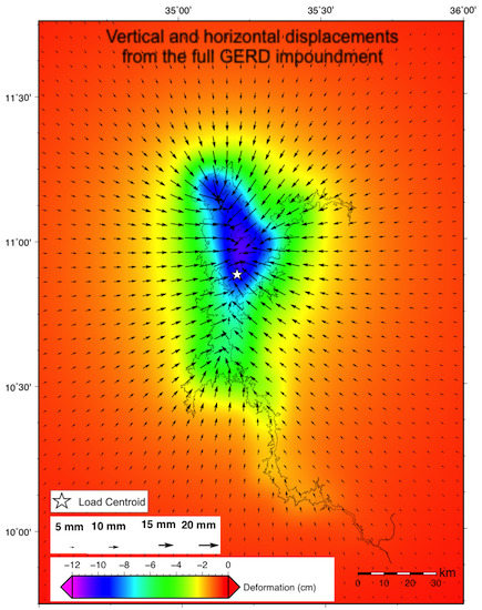
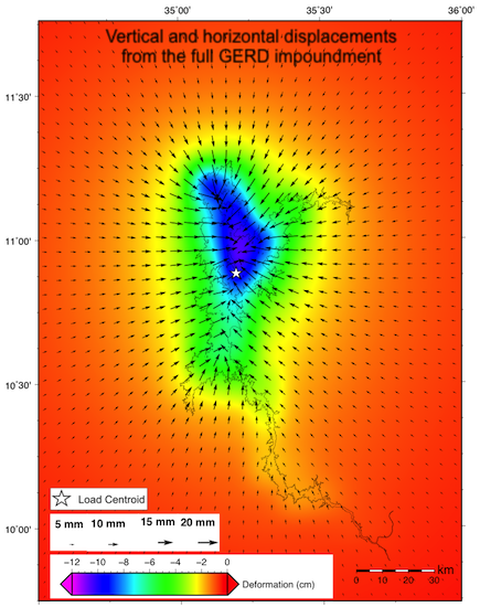
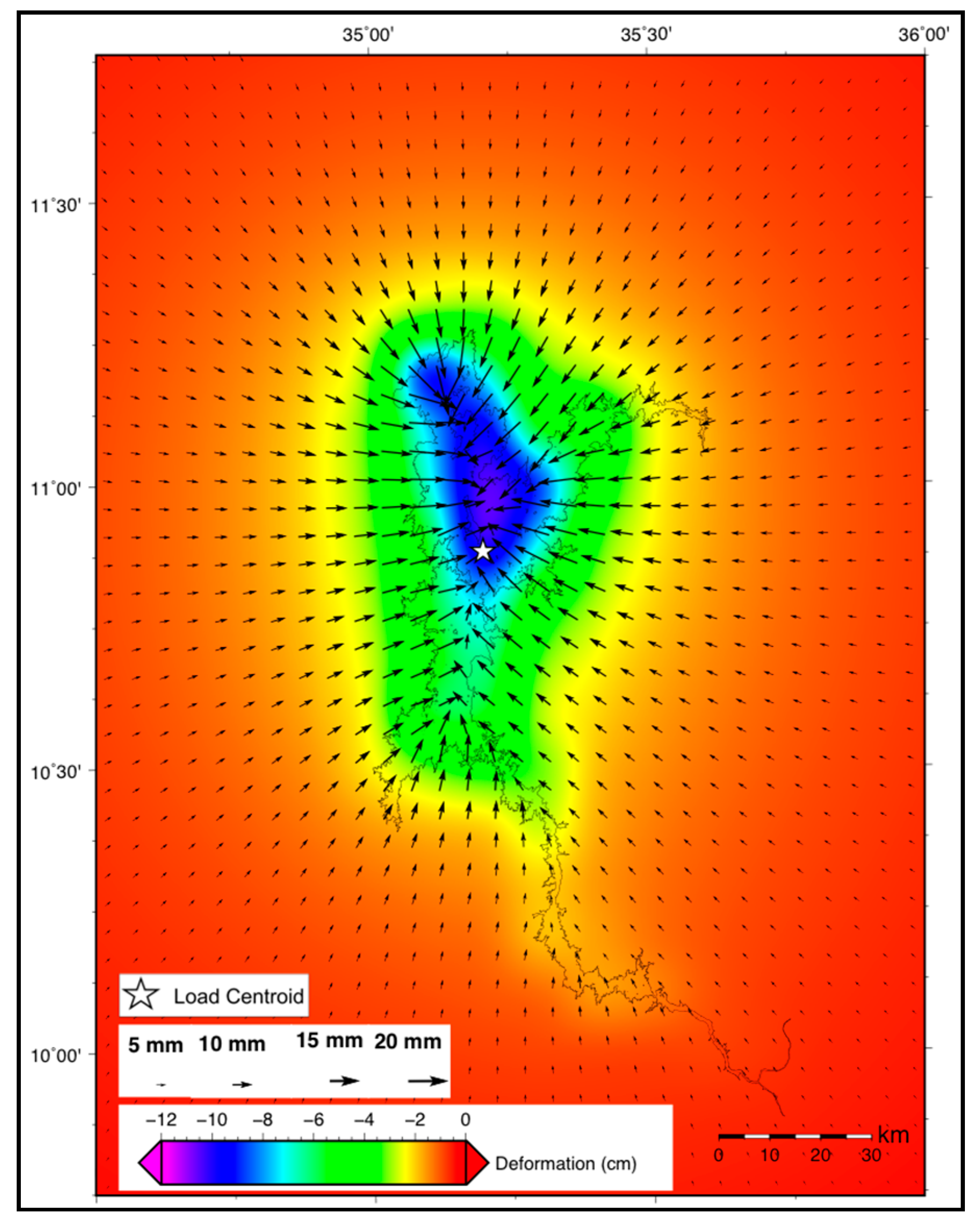
The maximum accumulated vertical and horizontal displacements from the SNREI model for the complete GERD impoundment utilizing the methods and datasets described in Section 2.1 and Section 2.2 are 11.99 and 1.99 cm, respectively. Figure 2 plots the total vertical and horizontal response from the entire hydrologic load from the full 140 m GERD impoundment. Vertical and horizontal displacements from the complete impoundment in excess of 1 cm extend out to ~99 and ~49 km from the 640 m weighted hydrologic load centroid, respectively. We point the reader to Video S1 for an animation showing the modeled flexural response along with its associated areal extent and water volume for each meter of water level rise from 500 to 640 m.
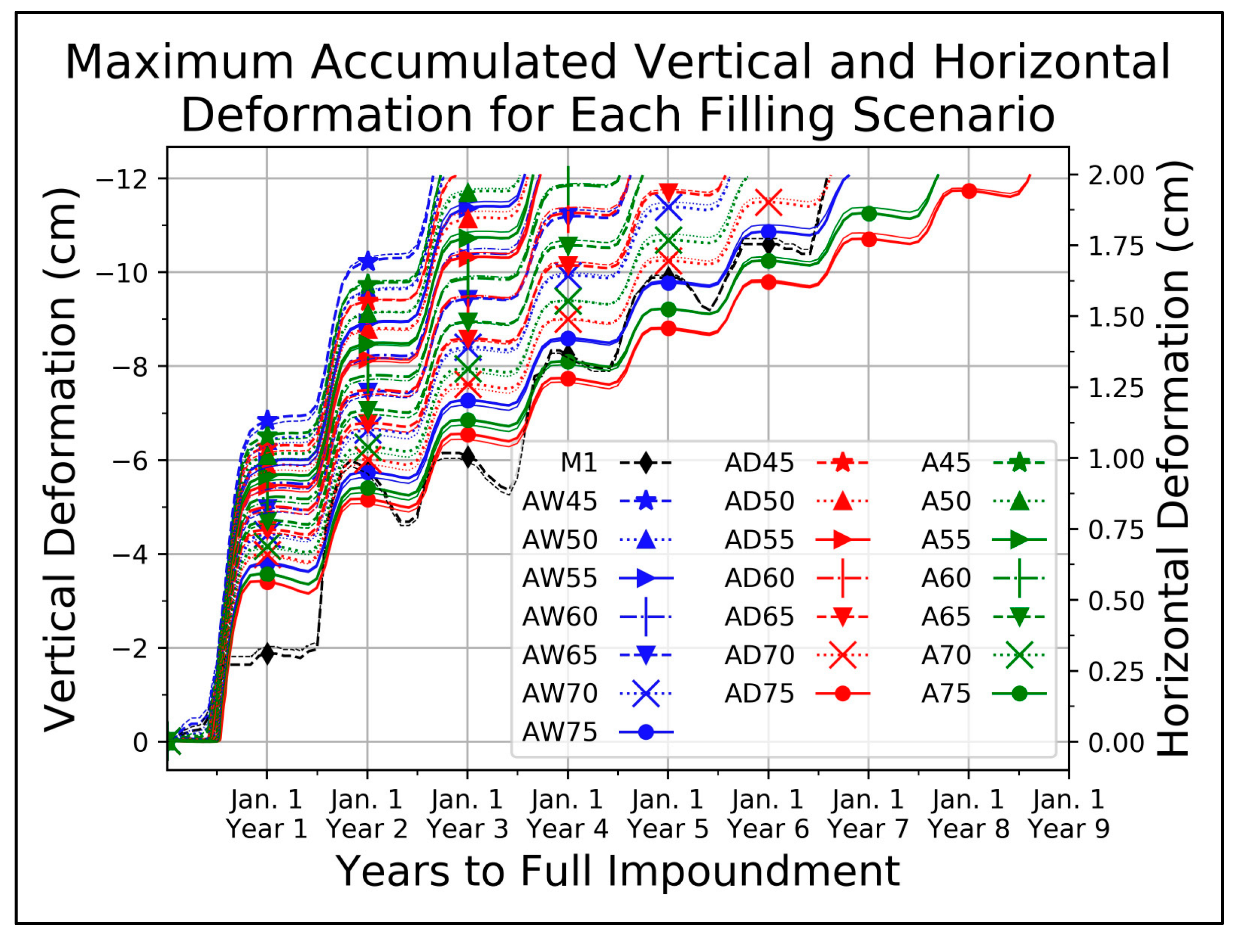
Figure 3 plots the daily accumulated horizontal and vertical displacements for each of the 22 different filling scenarios. We note that the vertical displacement for each of the filling scenarios maxes out at the same response due to the fact that we plot the accumulated displacement for the entire filling, and that according to [43], the elastic flexural response to any given load is both constant and instantaneous. That is to say, these maximum displacement values are the same for the vertical and horizontal displacements plotted in Figure 2.
3.2. Seasonal Operations
We derived the average monthly inflow, outflow, and water storage values for each of the five operational cycles, and plot them in Figure S8. We utilized these monthly hydrologic variables to derive an average annual regime of daily reservoir inflow and outflow rates, and subsequently the accumulated water levels and volumes for each of the five seasonal strategies (L1–L5). These are plotted in Figure S9. This figure shows that the maximum annual seasonal amplitudes of change for the areal extent, water level, and reservoir volume for each of the five average annual operational scenarios (L1–L5) are 491.12, 492.28, 484.33, 420.06, and 360.40 km2, 16.22, 16.25, 16.01, 14.13, and 12.22 m, and 23.09, 23.16, 22.76, 19.59, and 16.74 km3, respectively. We note that the percentage of the total accumulated water volume from the full impoundment for each average annual seasonal scenario is 25% (L1), 34% (L2), 34% (L3), 34% (L4), and 29% (L5). Similarly, we plot the daily water levels, water storage, and inflow and outflow rates for the five operational scenarios over their entire 39-year cycle in Figure S10. This figure shows that the maximum annual seasonal amplitudes of change for the areal extent, water level, and reservoir volume for each of the 39-year operational scenarios (L1–L5) are 902.02, 868.00, 821.83, 903.36, and 644.81 km2, 41.22, 36.99, 33.28, 46.53, and 26.88 m, and 36.46, 36.30, 35.22, 34.35, and 27.93 km3, respectively. We note that the percentages of the total accumulated water volume from the full impoundment for each of these maximum seasonal amplitudes from the full 39-year daily seasonal scenarios are 54% (L1), 54% (L2), 52% (L3), 51% (L4), and 41% (L5). This shows how large an effect dam operations can have on the amplitudes of seasonal hydrologic load fluctuations. In turn, these markedly different fluxes will determine the amplitude of flexural responses to the corresponding annual load changes in any given operational year, as discussed below.
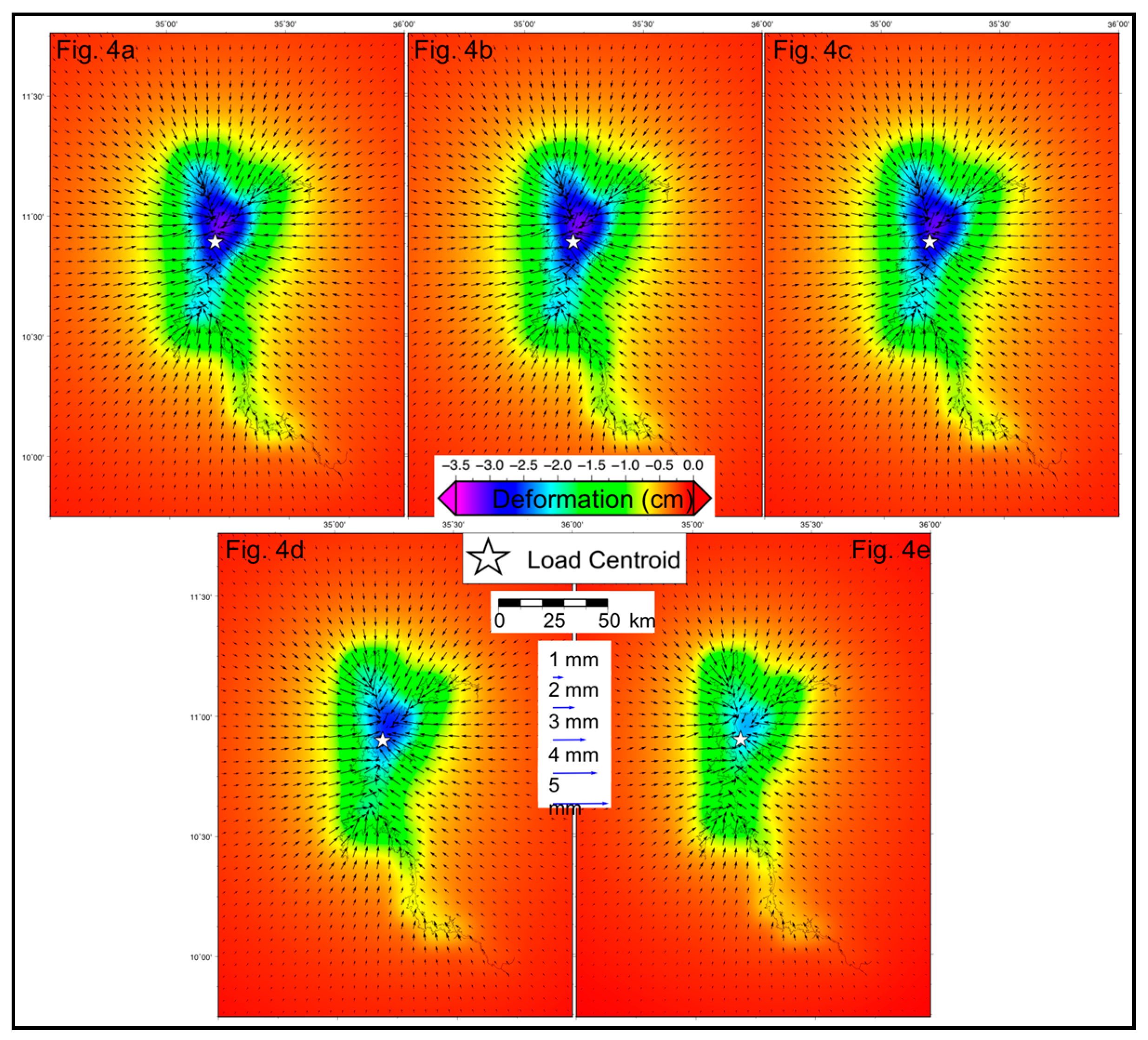
The maximum accumulated vertical (and horizontal) displacement from the SNREI model for each of the five average annual operational scenarios (L1–L5) is 3.27 (4.89), 3.29 (4.94), 3.24 (4.84), 2.76 (4.14), and 2.40 cm (3.59 mm), respectively. We plot the total vertical and horizontal response for these annual average operational scenarios (L1–L5) in Figure 4a–e. Vertical and horizontal displacements from the maximum seasonal amplitudes in excess of 1 cm and 3 mm for these five scenarios extend out to ~92 and ~51 km (L1–L3), ~77 and ~44 km (L4), and lastly ~49 and ~40 km (L5) from their respective maximum water level weighted hydrologic load centroids.
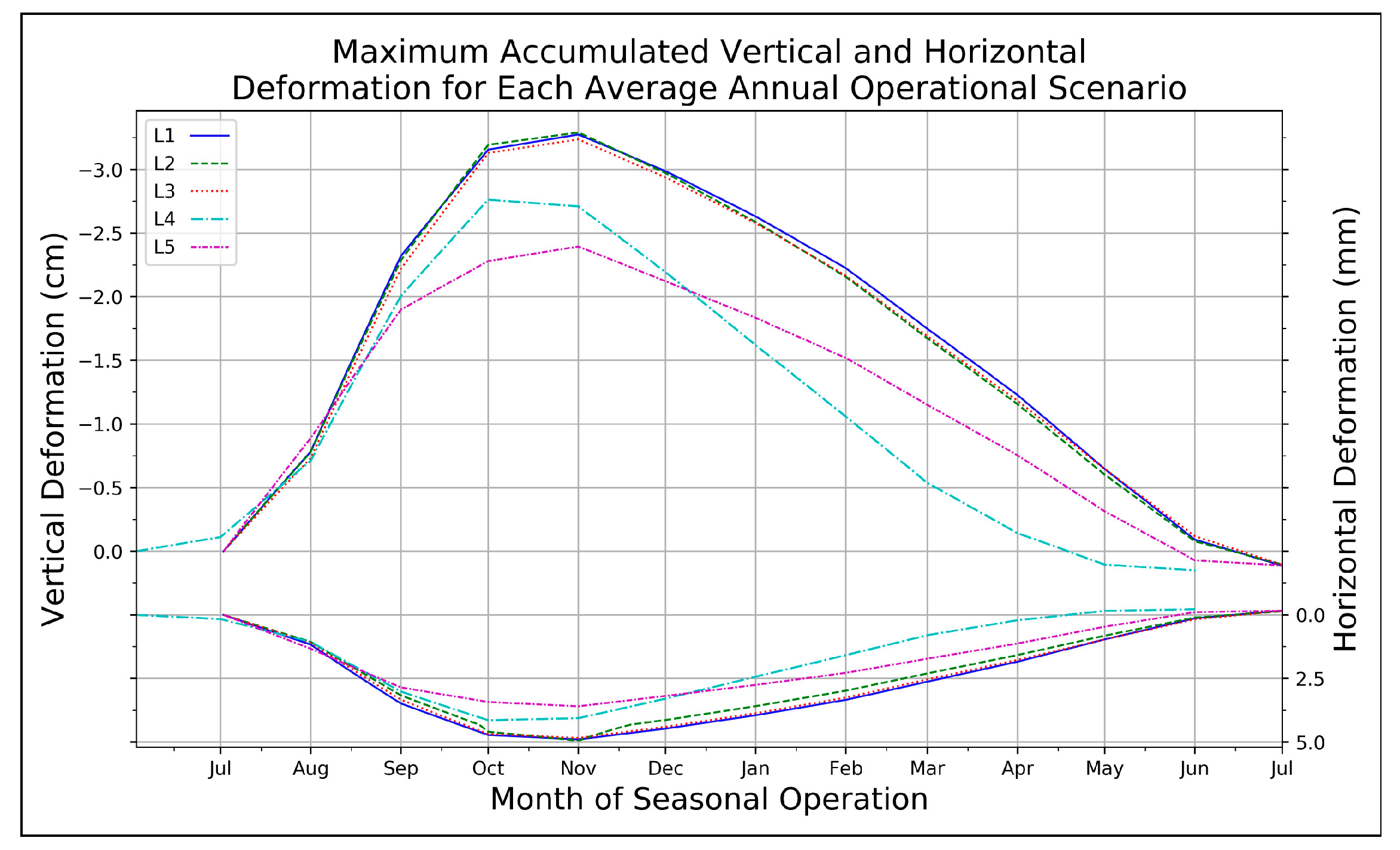
We plot the daily accumulated maximum horizontal and vertical displacements for each of the five seasonal operational scenarios in Figure 5. We note that the maximum accumulated displacements are the same as the responses plotted in Figure 4a–e. We also note that the maximum displacement for operational scenario L4 occurs one month prior to the other four scenarios. This is due to the operational start date of June 1 for the L4 scenario versus July 1 for the remaining four scenarios. Here, July 1 and June 1 are the first days in each scenario in which there is net positive reservoir storage.
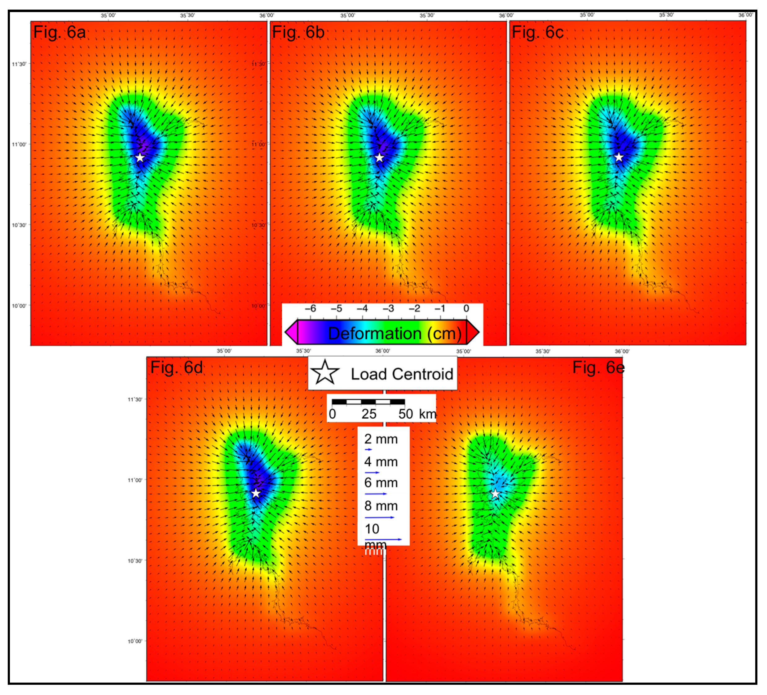
We note that the maximum accumulated vertical (and horizontal) displacement for each of the largest seasonal amplitudes of hydrologic change from the full 39-year dataset for the five operational scenarios (L1–L5) is 6.58 (9.39), 6.29 (8.94), 5.91 (8.45), 6.56 (9.58), and 4.61 cm (6.69 mm), respectively. We plot the total vertical and horizontal response for these maximum annual operational scenarios (L1–L5) in Figure 6a–e, respectively. Vertical and horizontal displacements from the maximum seasonal amplitudes in excess of 1 cm and 5 mm for these scenarios extend to ~78 and ~50 km (L1), ~93 and ~50 km (L2), ~93 and ~48 km (L3), ~78 and ~46 km (L4), and lastly ~78 and ~44 km (L5) from their respective maximum water level weighted hydrologic load centroids.
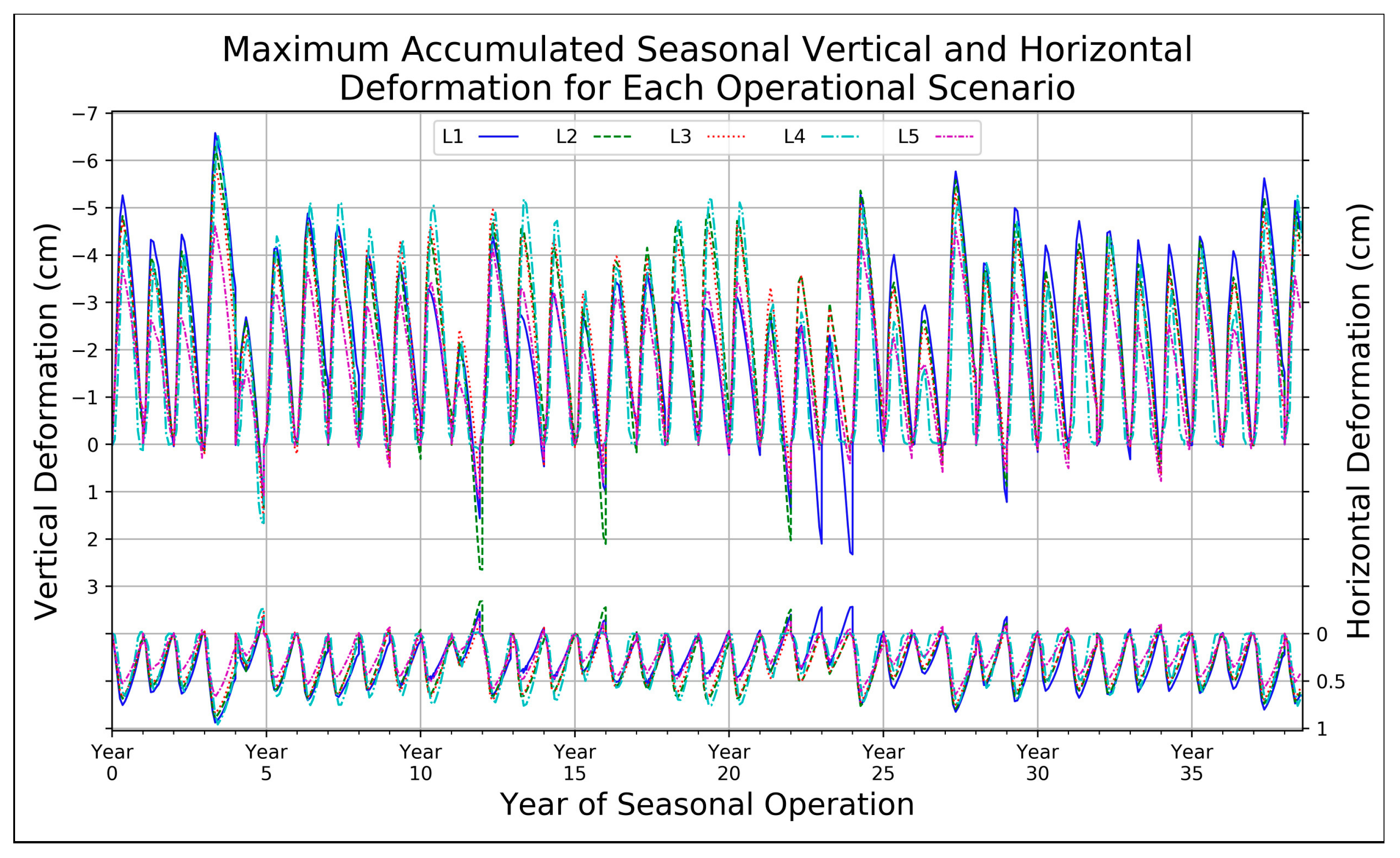
We plot the daily maximum vertical and horizontal accumulated flexural responses from the full 39-year dataset for each of the five scenarios in Figure 7. We start the water level for each of these runs such that the maximum water level over the full 39-year dataset is never greater than the maximum GERD water level of 640 m. We note that the seasonal maximum and minimum vertical and horizontal displacements for all five scenarios over all 39 years of hydrologic data are 6.58 and 1.32 cm (vertical) and 9.58 and 1.91 mm (horizontal), respectively. This further highlights the stark differences in the annual stresses applied on the crust from the varying hydrologic loading and unloading operational scenarios of the reservoir.
4. Discussion
4.1. Initial Impoundment
At present, our DSM-derived results cannot be validated to in situ or other remote sensing-based areal extent and volumetric water load curves of the GERD as the final impoundment process has not yet begun. However, our very high R-squared values of 0.99 are indicative of the quality of the relationships between water level, areal extent, and volumetric content (Figure S11a–c). These relationships can be employed by water managers and researchers to derive more meaningful operational rule curves and to better understand the hydrologic fluctuations as they relate to future GERD studies (e.g., remotely sensed volumetric calculations from ICESat-2, GRACE-FO, and SWOT). We note our method relies heavily on the DSM employed by our processing methodology, and that we have utilized the most accurate surface model (as compared to spatially overlapping ICESat GLAS pulses) at our disposal (Section 2.1).
For a comparison to the modeled vertical displacements from the full impoundment at the GERD (Figure 2), we note that vertical displacements from the full impoundment for two other large hydro-engineering projects (Lake Mead in the United States and the Three Gorges Reservoir in China) are ~12 cm and ~3.8 cm, respectively [46,47]. The locational difference in the maximum vertical displacement and the weighted hydrologic load centroid in Figure 2 is very likely caused by the upstream reaches of the GERD reservoir at this water level “pulling” the centroid toward the south-southeast away from the deformation center. Further, Video S1 shows the south-southeastward migration of the weighted hydrologic load centroid as the reservoir levels rise and the upstream reaches “pull” the centroids in that direction. We note that utilizing a different DSM than the one selected for this analysis would affect the displacements calculated from our flexural modeling methodology. The displacements from a given load are directly related to the input water levels at each cell in the DSM grid. As such, the overall difference in the modeled displacements from different DSMs would be dependent on the cell-by-cell differences in their water levels. We note that the results in Figure 2 and Video S1 are the total accumulated elastic flexural response from the GERD impoundment in its entirety. Further, we note that filling scenarios for reservoirs of this size are typically drawn out over several years/wet-dry seasons due to the size of the reservoir itself, downstream water users, and the seasonality of the inflows at the impoundment.
A filling plan has not been finalized for the GERD, and, as such, we focus our discussion on 22 (M1, A45–75, AW45–75, and AD45–75) of the 55 different scenarios as laid out in the end of Section 2.1. These particular filling scenarios were deemed the most realistic after comparing their outflow rates to the mean outflow at the impoundment site as well as their respective filling times. The former is important to negate downstream user impacts and the latter is important for the operation and timing of the reservoir operations. The filling time is also an important parameter where faster impoundments may increase the drained response that is responsible for the increase in diffusive pore pressure through the underlying rock. The filling scenarios had a start date of January 1, and for the most part, the first five months of each filling scenario shows little to no impoundment. We note that 14 of the 22 filling scenarios examined were complete before the fifth year, and that the shortest filling scenario (AW45) and the longest filling scenario (AD75) took ~2.65 and ~8.6 years, respectively.
Although the total magnitude of the vertical and horizontal displacements are the same for each filling scenario plotted in Figure 3, it is the timing of the hydrologic variables that play a role in the temporal dynamics of the load-induced flexural response. This is especially true for a marked seasonal hydrologic regime defined by a peak discharge lasting a few months followed by a low-flow period that we see at the GERD impoundment. This is evidenced in Figure 3 by the fact that 8 of the 22 filling scenarios (A45–55, AW45–55, and AD45–50) have nearly 50% (~6 and ~1 cm) of their total accumulated (~12 and ~2 cm) vertical and horizontal displacement (respectively) within the last half of the first year of the filling scenario. We point the reader to Dataset S1 for the complete displacement arrays for each of the 22 filling scenarios. We also note that all but one of the filling scenarios (M1) have more than 25% of their total deformation in the same six-month time span. However, if we think in terms of displacement per unit time and we take the quotient of the total accumulated vertical displacement and the filling time for each scenario plotted in Figure 3, we find that the top-five scenarios in terms of the lowest total daily displacement rate are AD75 (~0.04), A75 (~0.04), AW75 (~0.05), AD70 (~0.05), and M1 (~0.05 mm/day). In contrast, the bottom-five scenarios in terms of the highest total daily displacement rate are AW45 (~0.12), A45 (~0.12), AW50 (~0.12), AD45 (~0.11), and A50 (~0.09 mm/day). We note that because the total displacement is the same for each of the filling scenarios (500 to 640 m), these displacement rates are for the five longest and five shortest filling scenarios, respectively. We reiterate that the overall flexural response (Figure 2) from the full impoundment applied on the surrounding lithosphere will not occur within one season, but will be spread out over the filling scenario decided upon by the water managers. As such, we have shown (Figure 3) 22 different potential filling scenarios at the GERD, and how their associated flexural responses accumulate over their respective impoundment periods.
4.2. Seasonal Operations
Overall, the differences in accumulated horizontal and vertical displacements between the five operational scenarios plotted in Figure 5 stem from the different monthly (and subsequently, the daily) reservoir outflow rates. These scenarios are discussed at the end of Section 2.1 and are plotted in Figures S8 and S9, respectively. The different outflow rates are responsible for variations in monthly (and subsequently, the daily) water storage, and, in turn, the different areal extents and total water levels for each of the five scenarios. We expect there to be differences in the accumulated displacement from the different operational scenarios as the inputs into the elastic deformation models are the hydrologic load grids derived from these areal extents and water levels. The notable difference in both the timing and the quantity of reservoir outflow in scenarios L4 and L5 as compared with the outflow rates in scenarios L1–L3 causes the decreased accumulated displacement for scenarios L4 and L5 (See Figures S8 and S9).
We start the seasonal model runs at the first date in which there is positive reservoir storage (L1–L3, L5: July 1 and L4: June 1) and use a 622 m reservoir level as the initial model input. We selected the 622 m water level as [48] specified the minimum operating level of the GERD as such. However, other studies stated that the minimum operating level is at 590 m [49,50]. We ran our models with both 622 and 590 m as the starting point, and we note that the total volumetric change is the same in both runs and that the amplitudes of the seasonal water level and areal extent changes are larger with the 590 m elevation starting point. Further, the maximum accumulated vertical and horizontal displacements are around 1 cm and 1 mm larger (respectively) in the 590 m data runs as compared with the flexural results from the 622 m starting point. This is due to the increased load per unit area for the 590 m data runs as the reservoir volumes for both starting points are the same, but the maximum areal extents for the 590 m runs are smaller than their 622 m counterparts, thereby increasing the hydrologic load per unit area. In turn, this larger, more condensed loading affects the distance that the deformation extends from the corresponding load centroid as compared with the 622 m data runs. Here, we note that the vertical and horizontal displacements from the maximum seasonal amplitudes in excess of 1 cm and 3 mm for the scenarios with a 590 m water level start extend out to ~59 and ~50 km (L1–L2), ~59 and ~48 km (L3), ~48 and ~46 km (L4), and lastly ~49 and ~42 km (L5) from their respective maximum water level weighted hydrologic load centroids. This overall reduction in the spatial reach of the deformation as compared with the 622 m data runs is due to the abovementioned condensed hydrologic loading around the load centroid where the 590 m data runs do not have the increased displacement in the upstream (southerly) reaches of the reservoir.
The vertical and horizontal displacements plotted in Figure 7 are normalized to the first day of the seasonal cycle. Here, we define the beginning of an annual seasonal cycle as the first day in which there is positive water storage and the end to that cycle occurs when the water storage flips from negative to positive (i.e., a full seasonal inflow and outflow curve). The daily vertical displacement plotted in Figure 7 is the accumulated vertical response for that season at the location of maximum deformation for that annual cycle. Here, vertical displacement that is greater than zero indicates that the daily water level has dropped below the water level at the start of our defined seasonal cycle, and the accumulated displacement switches sign to a positive value due to the continued withdrawal of reservoir water (decreased water storage) and the subsequent upward flexural response (relaxation) of the crust. The decrease in water storage and subsequent crustal relaxation for each seasonal cycle begins after the maximum accumulated vertical displacement peak on the seasonal curves plotted in Figure 7 and ends when the reservoir storage changes from a positive to a negative value. The horizontal displacement is nearly always positive, and, similar to the plotted vertical displacement, it switches signs when the daily water level has dropped below the water level at the start of our defined seasonal cycle. The horizontal response curves in Figure 7 show that the non-vertical crustal motion changes direction from towards the center of load mass during water storage and downward flexural response to away from the center of load mass during periods in the seasonal cycle that are dominated by a reduction in water storage and subsequent reservoir withdrawals. This occurs simultaneously with the decrease in water storage and subsequent crustal relaxation for each seasonal cycle and begins after the maximum accumulated vertical displacement peak on the seasonal curves.
We note that the full vertical and horizontal displacement for each of the five average annual operational strategies (L1–L5) is 27%, 27%, 27%, 23%, and 20% and 24%, 25%, 24%, 21%, and 18% of the total maximum accumulated vertical and horizontal displacement from the entire GERD impoundment, respectively. In context, the vertical and horizontal percent differences for the highest amplitude year of the 39-year data cycle are 55%, 52%, 49%, 55%, and 38% and 47%, 45%, 43%, 48%, and 34%, respectively. The overall magnitude of the vertical and horizontal displacements for the five operational scenarios are highly varied when looking at both the average scenarios and the full 39-year runs. The deformation is dependent on the annual load density and the input natural hydrologic variables (e.g., inflow, seepage, actual ET) for that particular water year as well as the operational variables (i.e., outflow/reservoir release as it is related to hydropower generation) that the water managers decide upon. Subsequently, these varied reservoir inflow and outflow rates and release timings can dramatically affect the maximum accumulated seasonal displacement as well as the distance with which the flexural response occurs away from the associated hydrologic load centroid.
5. Conclusions
This study has compared the accuracy of several widely used DSMs to spaceborne laser altimetric products from the ICESat GLAS sensor in order to determine the most appropriate product for reservoir extent and volumetric calculations at the GERD. We utilized the ALOS-derived AW3D30 surface model to determine that the overall extent and total hydrologic load of the full GERD impoundment, which are ~1763.30 km2 and 67.37 km3 (Gt), respectively. We determined the areal extent and volumetric content for the GERD impoundment at 1 m water level increments (from 500 to 640 m) and derived hypsometric curves for water level versus areal extent and water load along with areal extent versus water load. We determined the most appropriate cubic and quadratic fits of these curves and found very high R-squared values for each. We utilized the associated coefficients to derive areal extent and volumetric content at sub-meter water level changes (e.g., 0.001 m) for each day in our scenarios.
We created daily water level, areal extent, water storage, inflow, and outflow values for 55 different filling scenarios as well as for 5 different operational strategies at the GERD. The time to full impoundment varies by scenario, and ranges from 1.6 to 76.7 years. We determined that the accumulated annual storage for these scenarios ranges from 0.9 to 48.3 km3 at the longer end of impoundment time to the shorter end, respectively. A more realistic scenario is, of course, somewhere in between these values. The accumulated annual reservoir storage during the initial impoundment directly affects the time it takes to fill the reservoir to its maximum water level of 640 m. We found that the maximum seasonal amplitude of reservoir load changes for each of the five operational strategies to consist of 54%, 54%, 52%, 51%, and 41% of the total accumulated water volume from the full impoundment. When compared with the percentages from the average annual operational strategies of 25%, 34%, 34%, 34%, and 29%, it becomes quite evident that reservoir operations have a large effect on the amplitude of seasonal hydrologic load fluctuations.
We found the maximum accumulated vertical and horizontal displacements caused by the hydrologic load from the full GERD impoundment to be 11.99 and 1.99 cm, and that the vertical and horizontal displacements in excess of 1 cm extend out to ~99 and 49 km from the 640 m weighted hydrologic load centroid, respectively. We derived the daily accumulated vertical and horizontal displacements for 22 of the 55 filling scenarios. Although the total magnitude of the elastic vertical and horizontal displacements are the same for each of the filling scenarios, it is the timing of these forces that play a role in the temporal dynamics of the load-induced flexural response. We note that the marked seasonal hydrologic regime at the GERD impoundment plays a major role in the timing of the deformation, and this is evidenced by the fact that 8 of the 22 filling scenarios (A45-55, AW45-55, and AD45-50) have nearly 50% (~6 and ~1 cm) of their total accumulated (~12 and ~2 cm) vertical and horizontal displacements (respectively) within the last half of the first year of the filling scenario.
We found that the maximum accumulated vertical (and horizontal) displacement for each of the largest seasonal amplitudes of hydrologic change from the full 39-year dataset for the five operational scenarios (L1 – L5) is 6.58 (9.39), 6.29 (8.94), 5.91 (8.45), 6.56 (9.58), and 4.61 cm (6.69 mm), respectively. The vertical and horizontal displacements in excess of 1 cm and 5 mm from these maximum amplitudes extend to ~78 and ~50 km (L1), ~93 and ~50 km (L2), ~93 and ~48 km (L3), ~78 and ~46 km (L4), and lastly ~78 and ~44 km (L5) from their respective maximum water level weighted hydrologic load centroids. We compared this maximum seasonal displacement to the displacements from the full impoundment and found that the vertical and horizontal percent differences for the highest amplitude year of the 39-year data cycle for the five operational scenarios are 55%, 52%, 49%, 55%, and 38% and 47%, 45%, 42%, 48%, and 34%, respectively. We determined that the seasonal maximum and minimum vertical and horizontal displacements for all five operational scenarios over all 39 years of hydrologic data are 6.58 and 1.32 cm (vertical) and 9.58 and 1.91 mm (horizontal), respectively. We have shown that the overall magnitude of the vertical and horizontal displacements for the five operational scenarios are highly varied, and that the deformation is dependent on the input natural hydrologic variables (e.g., inflow, seepage, actual ET) for that particular water year as well as the operational variables (i.e., outflow/reservoir releases as they are related to hydropower generation) that the water managers decide upon. Subsequently, we noted that the annual load density along with the varied reservoir inflow and outflow rates and release timings can dramatically affect the maximum accumulated seasonal displacement as well as the distance with which the flexural response occurs away from the associated hydrologic load centroid.
Supplementary Materials
The following are available online at https://www.mdpi.com/2072-4292/12/11/1886/s1, Figure S1: Monthly inflow, outflow, and water storage values for each of the average (A) water year impoundment scenarios, Figure S2: Monthly inflow, outflow, and water storage values for each of the average-dry (AD) water year impoundment scenarios, Figure S3: Monthly inflow, outflow, and water storage values for each of the average-wet (AW) water year impoundment scenarios, Figure S4: Daily reservoir inflows and outflows along with the accumulated water levels and hydrologic loads for each of the average (A) water year impoundment scenarios, Figure S5: Daily reservoir inflows and outflows along with the accumulated water levels and hydrologic loads for each of the average-dry (AD) water year impoundment scenarios, Figure S6: Daily reservoir inflows and outflows along with the accumulated water levels and hydrologic loads for each of the average-wet (AW) water year impoundment scenarios, Figure S7: Daily-accumulated water levels and hydrologic loads for the M1 impoundment scenario, Figure S8: Average monthly inflow, outflow, and water storage values for each of the five seasonal reservoir operation strategies, Figure S9: Average annual regime of daily reservoir inflow and outflow rates and the accumulated water levels and reservoir volumes for each of the five seasonal reservoir operation strategies, Figure S10: Daily water levels, water storage, and inflow and outflow rates for the five operational scenarios over their entire 39-year cycle, Figure S11: Hypsometric curves for water level versus areal extent and water load along with areal extent versus water load. Table S1: Areal extent and volumetric water loads for every meter of water level from 500 m to 640 m calculated from each of the five DSMs. Table S2: Annual outflow and inflow rates, accumulated reservoir storage, and the filling times for each impoundment scenario. Video S1: Animation displaying the flexural response along with the accumulated areal extent and hydrologic load for every meter of reservoir level rise from 500 m to the full impoundment of 640 m. Dataset S1; Zipped folder containing vertical and horizontal displacement arrays for each of the 22 different filling scenarios.
Author Contributions
Conceptualization, A.M.; methodology, A.M.; software, A.M.; validation, A.M.; formal analysis, A.M.; investigation, A.M.; resources, A.M.; data curation, A.M.; writing—original draft preparation, A.M.; writing—review and editing, A.M., Y.S.; visualization, A.M.; supervision, Y.S.; project administration, A.M.; funding acquisition, Y.S. All authors have read and agreed to the published version of the manuscript.
Funding
A portion of this research was funded by NASA’s Surface Water and Ocean Topography (SWOT) Program, grant number NNX16AH85G.
Acknowledgments
We thank Stefan Liersch for kindly supplying his monthly hydrologic data. Some figures in this paper were made with Generic Mapping Tools (GMT) software. This work used computational and storage services associated with the Hoffman2 Shared Cluster provided by the UCLA Institute for Digital Research and Education’s Research Technology Group. We thank Frank Madson for his help in figure creation.
Conflicts of Interest
The authors declare no conflict of interest. The funders had no role in the design of the study; in the collection, analyses, or interpretation of data; in the writing of the manuscript, or in the decision to publish the results.
References
- Zhang, Y.; Erkyihum, S.T.; Block, P. Filling the GERD: Evaluating Hydroclimatic Variability and Impoundment Strategies for Blue Nile Riparian Countries. Water Int. 2016, 41, 593–610. [Google Scholar] [CrossRef]
- Abtew, W.; Dessu, S.B. The Grand Ethiopian Renaissance Dam on the Blue Nile; Springer: Berlin/Heidelberg, Germany, 2018. [Google Scholar]
- Bureau of Reclamation, U.S. Department of Interior. Land and Water Resources of the Blue Nile Basin, Ethiopia; Main Report and Appendices; U.S. Government Printing Office: Washington DC, USA, 1964.
- Ahmed, A.T.; Elsanabary, M.H. Environmental and Hydrological Impacts of Grand Ethiopian Renaissance Dam on the Nile River. Int. Water Technol. J. 2015, 5, 260–271. [Google Scholar]
- Mulat, A.G.; Moges, S.A.; Moges, M.A. Evaluation of multi-storage hydropower development in the upper Blue Nile River (Ethiopia): Regional perspective. J. Hydrol. Reg. Stud. 2018, 16, 1–14. [Google Scholar] [CrossRef]
- Sharaky, A.M.; Hamed, K.H.; Mohamed, A.B. Model-Based Optimization for Operating the Ethiopian Renaissance Dam on the Blue Nile River; Springer: Cham, Switzerland, 2017. [Google Scholar]
- Liersch, S.; Koch, H.; Hattermann, F.F. Management Scenarios of the Grand Ethiopian Renaissance Dam and Their Impacts under Recent and Future Climates. Water 2017, 9, 728. [Google Scholar] [CrossRef] [Green Version]
- Melesse, A.M.; Abtew, W.; Setegn, S.G. Nile River Basin: Ecohydrological Challenges, Climate Change and Hydropolitics; Springer Science & Business Media: New York, NY, USA, 2014. [Google Scholar]
- Abtew, W.; Melesse, A.M.; Dessalegne, T. Spatial, inter and intra-annual variability of the Upper Blue Nile Basin rainfall. Hydrol. Process. Int. J. 2009, 23, 3075–3082. [Google Scholar] [CrossRef]
- Wheeler, K.G.; Basheer, M.; Mekonnen, Z.T.; Eltoum, S.O.; Mersha, A.; Abdo, G.M.; Zagona, E.A.; Hall, J.W.; Dadson, S.J. Cooperative Filling Approaches for the Grand Ethiopian Renaissance Dam. Water Int. 2016, 41, 611–634. [Google Scholar] [CrossRef]
- Beyene, A. Reflections on the Grand Ethiopian Renaissance Dam. Horn Afr. News 2013, 14, 2016. [Google Scholar]
- Zhang, L.; Yang, D.; Liu, Y.; Che, Y.; Qin, D. Impact of impoundment on groundwater seepage in the Three Gorges Dam in China based on CFCs and stable isotopes. Environ. Earth Sci. 2014, 72, 4491–4500. [Google Scholar] [CrossRef]
- Zhao, Y.; Li, Y.; Zhang, L.; Wang, Q. Groundwater level prediction of landslide based on classification and regression tree. Geod. Geodyn. 2016, 7, 348–355. [Google Scholar] [CrossRef] [Green Version]
- Paronuzzi, P.; Rigo, E.; Bolla, A. Influence of filling–drawdown cycles of the Vajont reservoir on Mt. Toc slope stability. Geomorphology 2013, 191, 75–93. [Google Scholar] [CrossRef]
- Zhang, M.; Dong, Y.; Sun, P. Impact of reservoir impoundment-caused groundwater level changes on regional slope stability: A case study in the Loess Plateau of Western China. Environ. Earth Sci. 2012, 66, 1715–1725. [Google Scholar] [CrossRef]
- Fredlund, D.G.; Rahardjo, H. Soil Mechanics for Unsaturated Soils; John Wiley & Sons: New York, NY, USA, 1993. [Google Scholar]
- Xia, M.; Ren, G.M.; Zhu, S.S.; Ma, X.L. Relationship between landslide stability and reservoir water level variation. Bull.Eng. Geol. Environ. 2015, 74, 909–917. [Google Scholar] [CrossRef]
- Allen, C.R. Reservoir-induced earthquakes and engineering policy. Rev. Geofísica 1980, 13, 20–24. [Google Scholar]
- Talwani, P. On the nature of reservoir-induced seismicity. In Seismicity Associated with Mines, Reservoirs and Fluid Injections; Springer: Berlin/Heidelberg, Germany, 1997; pp. 473–492. [Google Scholar]
- Kerr, R.A.; Stone, R. A human trigger for the great quake of Sichuan? Science 2009, 323, 322. [Google Scholar]
- Ge, S.; Liu, M.; Lu, N.; Godt, J.W.; Luo, G. Did the Zipingpu reservoir trigger the 2008 Wenchuan earthquake? Geophys. Res. Lett. 2009, 36. [Google Scholar] [CrossRef]
- Gahalaut, K.; Gupta, S.; Gahalaut, V.K.; Mahesh, P. Influence of Tehri Reservoir Impoundment on Local Seismicity of Northwest Himalaya. Bull. Seismol. Soc. Am. 2018, 108, 3119–3125. [Google Scholar] [CrossRef]
- Chander, R.; Chander, K. Probable influence of Tehri reservoir load on earthquakes of the Garhwal Himalaya. Curr. Sci. 1996, 70, 291–299. [Google Scholar]
- Enzminger, T.L.; Small, E.E.; Borsa, A.A. Accuracy of snow water equivalent estimated from GPS vertical displacements: A synthetic loading case study for western US mountains. Water Resour. Res. 2018, 54, 581–599. [Google Scholar] [CrossRef]
- Tregoning, P.; Watson, C.; Ramillien, G.; McQueen, H.; Zhang, J. Detecting hydrologic deformation using GRACE and GPS. Geophys. Res. Lett. 2009, 36. [Google Scholar] [CrossRef] [Green Version]
- Dumka, R.; Choudhury, P.; Gahalaut, V.K.; Gahalaut, K.; Yadav, R.K. GPS Measurements of Deformation Caused by Seasonal Filling and Emptying Cycles of Four Hydroelectric Reservoirs in India. Bull. Seismol. Soc. Am. 2018, 108, 2955–2966. [Google Scholar] [CrossRef]
- Neelmeijer, J.; Schöne, T.; Dill, R.; Klemann, V.; Motagh, M. Ground Deformations around the Toktogul Reservoir, Kyrgyzstan, from Envisat ASAR and Sentinel-1 Data—A Case Study about the Impact of Atmospheric Corrections on InSAR Time Series. Remote Sens. 2018, 10, 462. [Google Scholar] [CrossRef] [Green Version]
- Madson, A.; Sheng, Y.; Song, C. ICESat-derived lithospheric flexure as caused by an endorheic lake’s expansion on the Tibetan Plateau and the comparison to modeled flexural responses. J. Asian Earth Sci. 2017, 148, 142–152. [Google Scholar] [CrossRef]
- Gahalaut, V.K.; Yadav, R.K.; Sreejith, K.M.; Gahalaut, K.; Bürgmann, R.; Agrawal, R.; Sati, S.P.; Bansal, A. InSAR and GPS measurements of crustal deformation due to seasonal loading of Tehri reservoir in Garhwal Himalaya, India. Geophys. J. Int. 2017, 209, 425–433. [Google Scholar] [CrossRef]
- Borsa, A.A.; Agnew, D.C.; Cayan, D.R. Ongoing drought-induced uplift in the western United States. Science 2014, 345, 1587–1590. [Google Scholar] [CrossRef] [PubMed]
- Kraner, M.L.; Holt, W.E.; Borsa, A.A. Seasonal nontectonic loading inferred from cGPS as a potential trigger for the M6. 0 South Napa earthquake. J. Geophys. Res. Solid Earth 2018, 123, 5300–5322. [Google Scholar] [CrossRef]
- Tadono, T.; Ishida, H.; Oda, F.; Naito, S.; Minakawa, K.; Iwamoto, H. Precise global DEM generation by ALOS PRISM. Isprs Ann. Photogramm. Remote Sens. Spat. Inf. Sci. 2014, 2, 71. [Google Scholar] [CrossRef] [Green Version]
- NASA/METI/AIST/Japan Spacesystems; U.S./Japan ASTER Science Team. ASTER Global Digital Elevation Model; NASA EOSDIS Land Processes DAAC: Washington, DC, USA, 2009. [Google Scholar]
- Farr, T.G.; Rosen, P.A.; Caro, E.; Crippen, R.; Duren, R.; Hensley, S.; Kobrick, M.; Paller, M.; Rodriguez, E.; Roth, L.; et al. The shuttle radar topography mission. Rev. Geophys. 2007, 45. [Google Scholar] [CrossRef] [Green Version]
- Zwally, H.J.; Schutz, R.; Hancock, D.; Dimarzio, J. GLAS/ICESat L2 Global Land Surface Altimetry Data, Version 34; National Snow & Ice Data Center: Boulder, CO, USA, 2014; p. 10. [Google Scholar]
- Tadono, T.; Nagai, H.; Ishida, H.; Oda, F.; Naito, S.; Minakawa, K.; Iwamoto, H. Generation of the 30 m-Mesh Global Digital Surface Model by ALOS PRISM. Int. Arch. Photogramm. Remote Sens. Spat. Inf. Sci. 2016, 41, 157–162. [Google Scholar] [CrossRef]
- Laske, G.; Masters, G.; Ma, Z.; Pasyanos, M. Update on CRUST1. 0—A 1-degree global model of Earth’s crust. In Geophysical Research Abstracts; EGU General Assembly: Vienna, Austria, 2013. [Google Scholar]
- Kustowski, B.; Ekström, G.; Dziewoński, A. Anisotropic shear-wave velocity structure of the Earth’s mantle: A global model. J. Geophys. Res. Solid Earth 2008, 113. [Google Scholar] [CrossRef]
- Chen, J.; Pan, E.; Bevis, M. Accurate computation of the elastic load Love numbers to high spectral degree for a finely layered, transversely isotropic and self-gravitating Earth. Geophys. J. Int. 2017, 212, 827–838. [Google Scholar] [CrossRef]
- Pan, E.; Chen, J.Y.; Bevis, M.; Bordoni, A.; Barletta, V.R.; Molavi Tabrizi, A. An analytical solution for the elastic response to surface loads imposed on a layered, transversely isotropic and self-gravitating Earth. Geophys. Suppl. Mon. Not. R. Astron. Soc. 2015, 203, 2150–2181. [Google Scholar] [CrossRef] [Green Version]
- Love, A.E.H. Some Problems of Geodynamics: Being an Essay to which the Adams Prize in the University of Cambridge was Adjudged in 1911; CUP Archive: Cambridge, UK, 1911. [Google Scholar]
- Munk, W.H.; MacDonald, G.J. The rotation of the earth: A geophysical discussion. In The Rotation of the Earth: A Geophysical Discussion; Munk, W.H., MacDonald, G.J.F., Eds.; First Published 1960; Cambridge University Press: Cambridge, UK, 1975; xix + 323p. [Google Scholar]
- Farrell, W. Deformation of the Earth by surface loads. Rev. Geophys. 1972, 10, 761–797. [Google Scholar] [CrossRef]
- Melini, D.; Gegout, P.; Spada, G.; King, M. A Regional ElAstic Rebound Calculator. 2015. Available online: http://hpc.rm.ingv.it/rear/REAR-v1.0-User-Guide.pdf (accessed on 21 March 2020).
- Melini, D.; Spada, G.; Gegout, P.; King, M.A. REAR—A Regional ElAstic Rebound Calculator, User Manual for Version 1.0. 2014. Available online: https://www.researchgate.net/publication/275340197_REAR_a_Regional_ElAstic_Rebound_calculator (accessed on 21 March 2020).
- Kaufmann, G.; Amelung, F. Reservoir-induced deformation and continental rheology in vicinity of Lake Mead, Nevada. J. Geophys. Res. Solid Earth 2000, 105, 16341–16358. [Google Scholar] [CrossRef]
- Wang, H. Surface vertical displacements and level plane changes in the front reservoir area caused by filling the Three Gorges Reservoir. J. Geophys. Res. Solid Earth 2000, 105, 13211–13220. [Google Scholar] [CrossRef]
- Mulat, A.G.; Moges, S.A. Assessment of the impact of the Grand Ethiopian Renaissance Dam on the performance of the High Aswan Dam. J. Water Resour. Prot. 2014, 6, 583. [Google Scholar] [CrossRef] [Green Version]
- IpoE. International Panel of Experts (IPoE). Grand Ethiopian Renaissance Dam Project, Final Report; IpoE: Addis Ababa, Ethiopia, 2013. [Google Scholar]
- Jameel, A.L. The Grand Ethiopian Renaissance Dam: An Opportunity for Collaboration and Shared Benefits in the Eastern Nile Basin; Amicus Brief; World Water and Food Security Lab: Cambridge, MA, USA, 2014; pp. 1–17. [Google Scholar]
Figure 1.
Overview figure of the Grand Ethiopian Renaissance Dam (GERD) study area. The elevation of the GERD impoundment’s watershed is plotted on the right along with the global overview of the general location of the study area. The areal extent of the full GERD impoundment (640 m reservoir level) is plotted on the left along with the weighted hydrologic load centroid for the full water volume of the reservoir. The locations of the main dam and the saddle dam are also noted.

Figure 2.
Vertical and horizontal displacements from the full GERD impoundment. The modeled vertical displacement is plotted on the colored grid while the horizontal displacement motion vectors are plotted on top. The weighted hydrologic load centroid from the full reservoir volume is plotted as a star. The total areal extent of the full impoundment (640 m reservoir level) is drawn as a black polygon. These are the modeled elastic displacements from the full hydrologic loading for the entire GERD impoundment.

Figure 3.
Accumulated daily vertical and horizontal displacements from 22 different filling scenarios. The horizontal displacement on the second y-axis is marginally offset from the vertical displacement on the first y-axis and is plotted as the slightly minor lines of the same symbology for each of the filling scenarios.

Figure 4.
Vertical and horizontal displacements from each of the five average annual operational scenarios. The modeled vertical displacement is plotted on the colored grid while the horizontal displacement motion vectors are plotted on top. The maximum water level weighted hydrologic load centroids are plotted as stars. The maximum areal extent of the reservoir for each of these scenarios is drawn as a black polygon. (a–e) correspond to the average annual seasonal scenarios L1–L5, respectively. These are the maximum accumulated displacements for each of the five average annual operational scenarios.

Figure 5.
Maximum accumulated daily vertical and horizontal displacements from the five different average annual operational scenarios. Seasonal operations are started July 1 for scenarios L1–L3 and L5 and on June 1 for scenario L4. These are the first days in each scenario in which there is net positive reservoir storage. These plots track the daily displacement at the location of the overall maximum accumulated vertical and horizontal displacement for each average annual scenario. Note that the top and bottom portions of the plot correspond to vertical and horizontal displacement in cm and mm, respectively. We also note that the y-axis scale for the horizontal displacement is half that of the vertical displacement.

Figure 6.
Total vertical and horizontal displacements from the maximum annual amplitude for each of the five 39-year operational scenarios. The modeled vertical displacement is plotted on the colored grid while the horizontal displacement motion vectors are plotted on top. The maximum water level weighted hydrologic load centroids are plotted as stars, and the maximum areal extent of the reservoir for each of these scenarios is drawn as a black polygon. (a–e) correspond to the maximum displacement out of the full 39-year dataset for each of the five different seasonal operational scenarios (L1–L5).

Figure 7.
Maximum seasonal accumulated daily vertical and horizontal displacements for all five operational scenarios from the full 39-year datasets. These plots track the daily displacement at the location of the annual season’s overall maximum accumulated vertical and horizontal displacement for each scenario. The plotted data are the accumulated vertical and horizontal displacements for each seasonal cycle in the full 39-year dataset. Note that the displacement at the beginning of each season reverts back to zero, and the subsequent seasonal displacements are accumulated from that start point until the end of the season. The top and bottom portions of the plot correspond to vertical and horizontal displacement, respectively. We also note that the y-axis scale for the horizontal displacement is half that of the vertical displacement.


Table 1.
Mean absolute differences in elevation between the investigated digital surface models (DSMs) and spatially overlapping Ice, Cloud, and land Elevation Satellite (ICESat) Geoscience Laser Altimeter System (GLAS) pulses for all data, slopes ≤1°, ≤3°, ≤5°, and ≤10° along with their standard deviations.
| DSM | All: Mean Difference (SD) | 1°: Mean Difference (SD) | 3°: Mean Difference (SD) | 5°: Mean Difference (SD) | 10°: Mean Difference (SD) |
|---|---|---|---|---|---|
| ALOS | 4.61 m | 3.85 m | 3.74 m | 3.82 m | 3.77 m |
| (26.73 m) | (1.69 m) | (4.15 m) | (20.93 m) | (20.18 m) | |
| ASTER | 8.16 m | 6.32 m | 6.04 m | 6.42 m | 6.88 m |
| (27.20 m) | (4.29 m) | (5.73 m) | (21.28 m) | (20.65 m) | |
| SRTM_1arc | 5.47 m | 4.56 m | 4.74 m | 4.84 m | 4.75 m |
| (26.71 m) | (2.09 m) | (4.28 m) | (20.87 m) | (20.13 m) | |
| SRTM_3arc_nonVoid | 7.22 m | 4.60 m | 4.86 m | 5.07 m | 5.34 m |
| (27.17 m) | (2.23 m) | (4.46 m) | (20.92 m) | (20.24 m) | |
| SRTM_3arc_yesVoid | 7.22 m | 4.60 m | 4.86 m | 5.07 m | 5.34 m |
| (27.17 m) | (2.23 m) | (4.46 m) | (20.92 m) | (20.24 m) |
© 2020 by the authors. Licensee MDPI, Basel, Switzerland. This article is an open access article distributed under the terms and conditions of the Creative Commons Attribution (CC BY) license (http://creativecommons.org/licenses/by/4.0/).
Share and Cite
MDPI and ACS Style
Madson, A.; Sheng, Y. Reservoir Induced Deformation Analysis for Several Filling and Operational Scenarios at the Grand Ethiopian Renaissance Dam Impoundment. Remote Sens. 2020, 12, 1886. https://doi.org/10.3390/rs12111886
AMA Style
Madson A, Sheng Y. Reservoir Induced Deformation Analysis for Several Filling and Operational Scenarios at the Grand Ethiopian Renaissance Dam Impoundment. Remote Sensing. 2020; 12(11):1886. https://doi.org/10.3390/rs12111886
Chicago/Turabian StyleMadson, Austin, and Yongwei Sheng. 2020. "Reservoir Induced Deformation Analysis for Several Filling and Operational Scenarios at the Grand Ethiopian Renaissance Dam Impoundment" Remote Sensing 12, no. 11: 1886. https://doi.org/10.3390/rs12111886
Note that from the first issue of 2016, this journal uses article numbers instead of page numbers. See further details here.