Simulating Multi-Directional Narrowband Reflectance of the Earth’s Surface Using ADAM (A Surface Reflectance Database for ESA’s Earth Observation Missions)

Abstract

The ADAM (A Surface Reflectance Database for ESA’s Earth Observation Missions) product (a climatological database coupled to its companion calculation toolkit) enables users to simulate realistic hyperspectral and directional global Earth surface reflectances (i.e., top-of-canopy/bottom-of-atmosphere) over the 240–4000 nm spectral range (at 1-nm resolution) and in any illumination/observation geometry, at 0.1° × 0.1° spatial resolution for a typical year. ADAM aims to support the preparation of optical Earth observation missions as well as the design of operational processing chains for the retrieval of atmospheric parameters by characterizing the expected surface reflectance, accounting for its anisotropy. Firstly, we describe (1) the methods used in the development of the gridded monthly ADAM climatologies (over land surfaces: monthly means of normalized reflectances derived from MODIS observations in seven spectral bands for the year 2005; over oceans: monthly means over the 1999–2009 period of chlorophyll content from SeaWiFS and of wind speed from SeaWinds), and (2) the underlying modeling approaches of ADAM toolkit to simulate the spectro-directional variations of the reflectance depending on the assigned surface type. Secondly, we evaluate ADAM simulation performances over land surfaces. A comparison against POLDER multi-spectral/multi-directional measurements for year 2008 shows reliable simulation results with root mean square differences below 0.027 and R² values above 0.9 for most of the 14 land cover IGBP classes investigated, with no significant bias identified. Only for the “Snow and ice” class is the performance lower pointing to a limitation of climatological data to represent actual snow properties. An evaluation of the modeled reflectance in the specific backscatter direction against CALIPSO data reveals that ADAM tends to overestimate (underestimate) the so-called “hot-spot” by a factor of about 1.5 (1.5 to 2) for barren (vegetated) surfaces.

1. Introduction

In the solar spectral range (400–2500 nm) land surface reflectance is the major contributor to “at sensor” radiance measurements under clear sky conditions [1,2]. Earth surface reflectances are characterized by smooth temporal variations (opposite to atmospheric features with sharp absorption features) which are, to the first order, shaped by the absorbing properties of the surface constituents (e.g., photosynthetic and non-photosynthetic pigments for plant canopies and water surfaces, mineral composition for soils, water content, etc.). The surface reflectance also varies with the illumination and view geometry depending on the scattering generated by different “geometrical” factors of the medium considered: wave slopes for ocean surfaces which lead to a departure of the maximum reflectance from the “pure” specular direction (also known as sunglint), surface roughness and canopy structure (e.g., volume and spatial distribution of leaves and crowns) which shape the directional signature of soil, and vegetation reflectance (including the reflectance increase in the retro-solar direction known as the “hot spot” effect). Indeed, the reflectance of most natural surfaces is largely anisotropic in the solar spectral range. Snow reflectance is more isotropic, but nevertheless shows larger reflectance values in the forward scattering direction [3].

Unfortunately, the directionality of the surface reflectance is often neglected in operational algorithms dedicated to atmospheric correction or characterization of atmospheric properties. Indeed, the reflectance from these surfaces is often based on an assumption of Lambertian (isotropic) surfaces. Mostly, this is because it significantly simplifies the resolution of the radiative transfer [4]. This is the case, for instance, for the atmospheric correction scheme of the Moderate Resolution Imaging Spectroradiometer (MODIS) land surface reflectance products MOD09 [5]. The relative error on the estimated surface reflectance due to the Lambertian assumption depends on the observation geometries and the number of multi-angle observations considered, but it typically varies between 3–12% in the visible and 0.7–5.0% in the near-infrared [4], but can reach higher values up to 40% [6,7] depending on the waveband and observation direction. The assumption of Lambertian surfaces is also used for retrieval algorithms of aerosol properties, for example those applied over land to the MODIS [8,9], Medium Resolution Imaging Spectrometer (MERIS) [10,11], or Visible Infrared Imaging Radiometer Suite (VIIRS) [12] missions. Likewise, for trace-gas and cloud retrievals from passive nadir looking instrumentation, a Lambertian surface reflectivity is often assumed (e.g., [13,14,15,16,17]). Several of these algorithms share the use of an a priori climatological estimate of surface reflectivity that is Lambertian. It has been shown that neglecting the surface anisotropy can lead to substantial errors in the retrieval of NO₂ air mass factors (AMFs) [18,19] and vertical tropospheric columns [20], or cloud parameters (reflectivity, cloud fraction, cloud top pressure, air mass factor, etc.) [19,21,22]. The retrieval error increases with the contribution of the surface reflectivity to the “at sensor” radiance.

There is therefore an urgent need for accurate information on typical surface (top-of-canopy/bottom-of-atmosphere) reflectances, representing realistically the spectral and directional signatures of the Earth surfaces, in order to quantify the sensitivity of the retrieval to surface reflectance variability and to develop adaptation measures accounting for surface anisotropy including the use of geographically and temporal collocated surface reflectance information. In this context, the use of current Lambertian reflectance or albedo databases is reduced, because of their limited ability to reproduce the spectral and/or directional variations. The spectral information most commonly used is surface albedo databases which are also limited to the few broad-band channels of the instrument(s) they derive from, and these are provided for a typical observation geometry. This holds for the “classical” Lambertian equivalent reflectance (LER) databases [23,24,25,26], as well as several databases of (i) multi-spectral albedos (which differ from LER by the integration of the surface reflectance over the entire hemisphere) either inferred from MODIS [27], Multi-angle Imaging Spectroradiometer (MISR) [28], MERIS [21] or by the fusion of several instruments (e.g., GlobAlbedo, [29]), and (ii) multi-spectral reflectances corrected for the surface anisotropy every eight days from MODIS Collection 5 [30]. Multi-spectral/multi-directional datasets derived from POLDER (Polarization and Directionality of the Earth’s Reflectance) [31,32] or reflectance anisotropy parameters derived from MODIS (MCD43A1 BRDF (Bidirectional Reflectance Distribution Function)/Albedo Model Parameters Product [27]), characterizing the surface anisotropy, remain limited to specific broad-bands in the visible to near-infrared range. Another example is the daily MODIS spectral BRDF climatology derived at 1 km from Collection 6 for the time period 2000–2016 [33]. More recently, a land surface atlas was derived from MODIS data to simulate hyperspectral/directional reflectance within the 400–2500 nm range [1], but both this and the previous reference only apply to land surfaces.

It was therefore concluded that a monthly mean climatology of hyperspectral surface reflectances is needed for the whole Earth’s surface, which led to the initiation of the European Space Agency (ESA) study ADAM (A Surface Reflectance Database for ESA’s Earth Observation Missions). In ADAM, a monthly climatological database and a companion toolkit were designed to simulate realistic spectro-directional variations of the Earth’s surface reflectance at the global scale with a moderate 0.1° × 0.1° resolution (~10 × 10 km²). The ADAM database contains climatological data, which are used as input by ADAM stand-alone calculation toolkit application programming interface (API) to calculate hyperspectral/bidirectional reflectance (or bidirectional reflectance factor according to Schaepman-Strub and colleagues [34], which is unitless), over the 240–4000 nm spectral range, with a spectral resolution of 1 nm and given any illumination/observation geometry. ADAM (database and API) is freely available online, after registration, at http://adam.noveltis.fr.

Different datasets and processing algorithms are applied depending on the surface type. For land surfaces (soil/vegetation and snow), the ADAM database contains a climatology (monthly means) of normalized reflectances for a reference illumination/observation geometry in the seven MODIS land broad-bands, which are processed by the FondsDeSol (FDS) processing chain [30] from the MODIS MOD09 products (representative of year 2005) derived from Aqua and Terra observations. For water surfaces, the database is made of climatological data (over the 1999–2009 period) of (i) chlorophyll content derived from SeaWiFs (Sea-viewing Wide Field-of-view Sensor onboard OrbView-2) and (ii) surface wind speed from SeaWinds (onboard QuikSCAT). Pixels covered by sea ice are identified by the use of the CryoClim monthly mean ice cover information.

The ADAM API developed for interaction with the database enables the computation of the spectro-directional variation of the surface reflectance in any narrow-band/observation geometry using these datasets and relying on the following approaches:

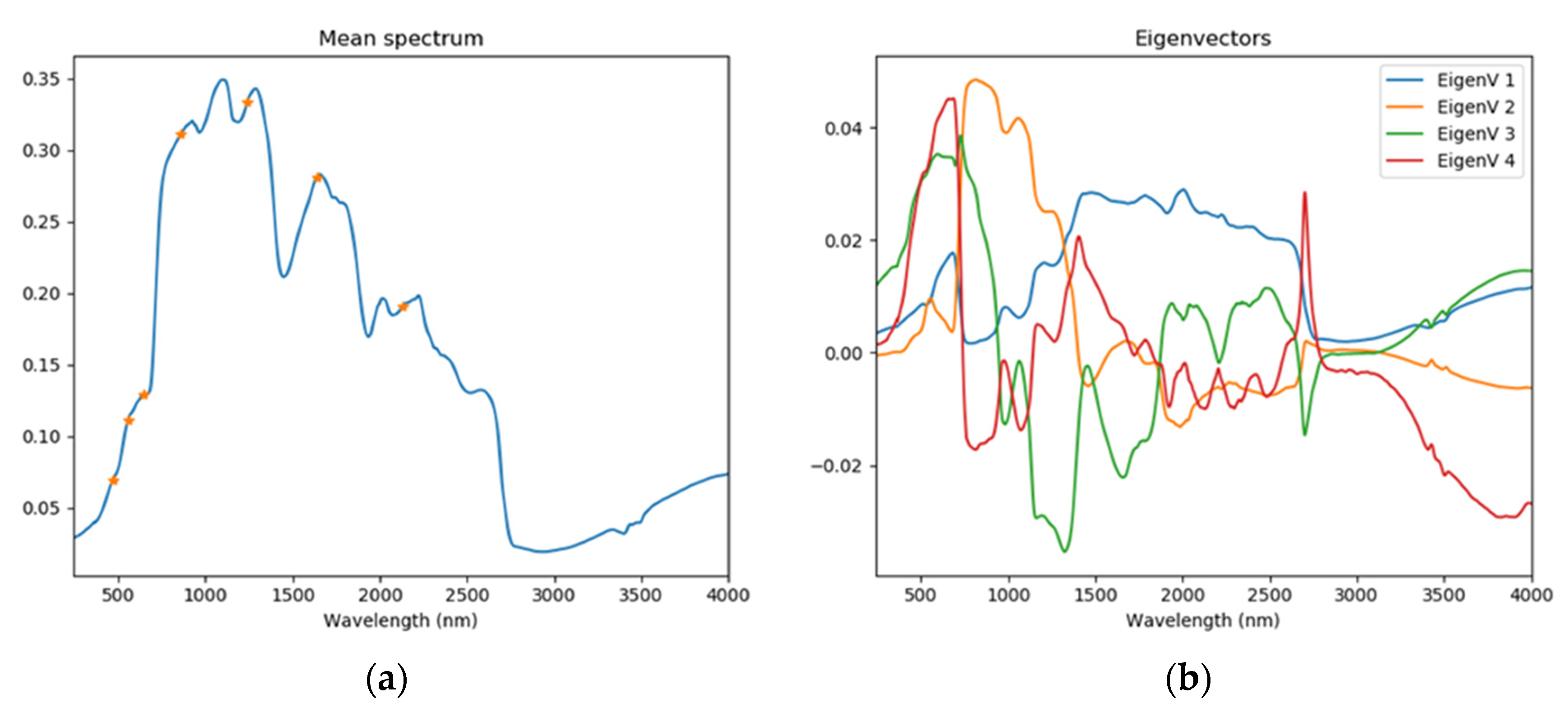
• For the soil/vegetation pixels, the spectral interpolation/extrapolation of the MODIS broad-bands/normalized reflectances between 240 and 4000 nm is performed using empirical orthogonal functions (EOFs) derived from spectral reflectance databases of soil/vegetation/leaf optical properties (similar to [1]). The Ross–Li-HS kernel based BRDF model [35] is used to calculate the reflectance spectrum in any illumination/observation geometry. A separate processing scheme is applied for snow covered surfaces: It relies on the Asymptotic Radiative Transfer (ART) model [36], fitted to the normalized reflectances, to simulate the spectro-directional variations of snow reflectance. Moreover, it is possible to calculate the uncertainty attached to the land surface reflectance: the calculation relies on the variance covariance matrix of the reflectance values between the seven MODIS bands for each 0.1° × 0.1° pixel.
• Over water surfaces, the reflectance is simulated by a combination of three components: (i) the water column and (ii) foam, that mainly shape reflectance spectral variations, and (iii) the specular reflection that essentially drives reflectance directionality. The water column reflectance is parameterized as a function of the chlorophyll content and specular reflection (also referred to as sunglint), which mostly depends on the wind speed.

In Section 2, we describe the reflectance models used in the ADAM API. Section 3 presents the data used for building the ADAM monthly climatology database over land and water surfaces and their processing (including the gap-filling approaches). In Section 4, we perform an evaluation of ADAM simulations of spectro-directional reflectances over land surfaces. In Section 5, we discuss the assumptions and limitations of ADAM, and present our concluding remarks in Section 6.

2. ADAM Spectral and Directional Calculation Models (API Toolkit)

Depending on the surface type, specific models are implemented in the ADAM calculation toolkit to simulate the spectro-directional variations of surface reflectance. Over land, the main input to the ADAM models is the ADAM climatological broadband MODIS-FDS reflectances (see Section 3.1) that are provided in a standard illumination and viewing geometry. The standard geometry is defined for a sun zenith angle θ_s of 45° and a viewing at nadir (i.e., the view zenith angle θ_v is 0°, in which case the relative azimuth angle ϕ is meaningless). Further, we define the backward scattering direction as ϕ = 0° while the forward scattering direction corresponds to ϕ = 180°.

The API calculation toolkit is written in Python3 and requires one input configuration file (in Python) to be provided by users. In this file, users may fill specific configuration keywords to parameterize the reflectance simulation. The keywords inform the API on the type of calculation to be performed (spectral calculation only, multi-directional reflectance or time-series calculations), the illumination/viewing geometry, the spatial coordinates of the area of interest, the month to be considered, the spectral range, etc. The baseline reflectance spectrum calculation is performed over the whole 240–4000 nm range at 1-nm (as described in the sections below). At the user’s request, the API can also output sampled narrowband reflectances in specific bands (by providing the name of a pre-defined instrument for instance) or calculate averaged broadband reflectances (by specifying the lower/upper limit of a spectral range of interest).

Here we recount the underlying principles of the ADAM models; additional details are provided in the Algorithm Theoretical Basis Document available at [37].

2.1. Land Surfaces

2.1.1. Vegetation and Soil

The generation of the reflectance spectrum over the 240–4000 nm domain at a 1-nm resolution by the ADAM API toolkit is performed by extrapolating the normalized surface reflectances (i.e., provided in the standard geometry described above) in seven MODIS broad-bands (see Section 3.1) using empirical orthogonal functions. The extrapolation of the spectral reflectances into any solar/viewing geometry is achieved thanks to the Ross–Li-HS semi-empirical BRDF model [35].

Spectral Modeling

Spectral calculation relies on the assumption that the reflectances for soil and vegetation are correlated across the 240–4000 nm range and that a few spectral measurements in the visible and near-infrared provide sufficient information on the reflectance in the UV (below 400 nm) and shortwave infrared (from 2500 nm to 4000 nm) [1,38,39,40]. That assumption is further supported by statistical analysis (results not presented here) of tens of spectra available from several databases, containing measured spectral reflectances from soil and vegetation samples (presented in Section 3.4.1).

The simulated reflectance spectrum ρ(λ)over the 240–4000 nm spectral range in the standard observation geometry is expressed as a function of an averaged spectrum $\overline{{\mathsf{\rho }}_{EOF}}(\mathsf{\lambda })$ and a few EOF eigenvectors ${{\mathsf{\rho }}_{EOF}}_v^j(\mathsf{\lambda })$ (centered), which are both derived from these databases (presented in Figure 1):

$$\mathsf{\rho }\left(\mathsf{\lambda },45°,0°,0°\right)=\overline{{\mathsf{\rho }}_{EOF}}(\mathsf{\lambda })+\sum _{j=1}^M{\alpha }_j{{\mathsf{\rho }}_{EOF}}_v^j(\mathsf{\lambda })$$

(1)

Only the first four eigenvectors (which contain 99% of the measured variance) were considered as their performance in terms of model-data reconstruction (over the measured reflectance spectra) was globally better compared to cases where either three or five eigenvectors were used instead. The weights ${\alpha }_j$ were calculated on a pixel/month basis in order to minimize the misfit between the simulated reflectances and the normalized MODIS-FDS reflectances in the seven broad-bands considered. D is the matrix of the four eigenvectors sampled at the MODIS band centers, $\overline{{\mathsf{\rho }}_{EOF}}\left({\mathsf{\lambda }}_{MODIS}\right)$ is the averaged spectrum sampled at the same wavelengths, and ${\mathsf{\rho }}_{ADAM}\left({\mathsf{\lambda }}_{MODIS}\right)$ is the MODIS-FDS surface reflectance measurements from the ADAM climatological database. The vector of the optimal weights is estimated as:

$$\mathsf{\alpha }=P.\left({\mathsf{\rho }}_{ADAM}\left({\mathsf{\lambda }}_{MODIS}\right)-\overline{{\mathsf{\rho }}_{EOF}}\left({\mathsf{\lambda }}_{MODIS}\right)\right) \mathrm{with} P={\left(D^{T}D\right)}^{-1}{D}^T$$

(2)

For each pixel/month, the uncertainty on the spectrally extrapolated spectrum can be calculated using the variance/covariances $B_{MODIS}$ of the reflectances in the seven MODIS channels (provided at all land pixels) (see Section 3.1) as the square root of the diagonal elements of the B covariance matrix defined as:

$$B=P.B_{MODIS}.P^T$$

(3)

Directional Modeling

The Ross–Li-HS [35] semi-empirical BRDF model represents the directional variation of land surface reflectance as the sum of three kernels: an isotropic component that varies spectrally, a geometric-optical surface scattering kernel (F₁), and a volumetric scattering kernel (F₂). F₁ and F₂ include the representation of the hot spot effect [41] (i.e., the reflectance increase in the retro-solar direction), with F₂ parameterized as a function of the phase angle and a characteristic angle ${\mathsf{\xi }}_0$ (set to 1.5°) related to the ratio of scattering element size and canopy vertical density [42]. The model was selected based on its higher fitting performances over various land surfaces (vegetation and soil) among several semi-empirical kernel driven models [35]. The F₁ and F₂ functions are given by:

$$F_1\left({\theta }_s,{\theta }_v,\varphi \right)=\frac{m}{\pi }\left(t-\sin t.\cos t-\pi \right)+\frac{1+\cos \mathsf{\xi }}{2\cos {\theta }_s\cos {\theta }_v}$$

(4)

$$F_2\left({\theta }_s,{\theta }_v,\varphi \right)=\frac{4}{3\pi }\frac{1}{\cos {\theta }_s+\cos {\theta }_v}\left[\left(\frac{\pi }{2}-\mathsf{\xi }\right)\cos \mathsf{\xi }+\sin \mathsf{\xi }\right]\times \left[1+{\left(1+\frac{\mathsf{\xi }}{{\mathsf{\xi }}_0}\right)}^{-1}\right]-\frac{1}{3}$$

(5)

where ξ is the phase angle, and $\mathsf{\Delta }\left({\theta }_s,{\theta }_v,\varphi \right)$ is the horizontal distance between the sun and view directions defined by: $\mathsf{\Delta }\left({\theta }_s,{\theta }_v,\varphi \right)=\sqrt{{\tan }^2{\theta }_s+{\tan }^2{\theta }_v-2\tan {\theta }_s\tan {\theta }_v\cos \varphi }$. t and m are defined as: $\cos t=\frac{2}{m}\sqrt{{\mathsf{\Delta }}^2+{\left(\tan {\theta }_s\tan {\theta }_v\sin \varphi \right)}^2}$ and $m=\frac{1}{\cos {\theta }_s}+\frac{1}{\cos {\theta }_v}$.

The surface reflectance in the $\left({\theta }_s,{\theta }_v,\varphi \right)$ observation geometry depends on the normalized reflectance at a given wavelength λ and in the standard geometry ($\rho \left(\mathsf{\lambda },45°,0°,0°\right)$) inferred from Equation (1), and the F₁ and F₂ kernels as:

$$\rho \left(\mathsf{\lambda },{\theta }_s,{\theta }_v,\varphi \right)=\rho \left(\mathsf{\lambda },45°,0°,0°\right)\frac{1+V{F}_1\left({\theta }_s,{\theta }_v,\varphi \right)+R{F}_2\left({\theta }_s,{\theta }_v,\varphi \right)}{1+V{F}_1\left(45°,0°,0°\right)+R{F}_2\left(45°,0°,0°\right)}$$

(6)

where the parameters V and R control the amplitude of the two kernels. They are estimated on a per pixel per month (written hereafter as pixel/month) basis as a linear function of the isotropic reflectance $\rho \left(\mathsf{\lambda },45°,0°,0°\right)$ so as to account for the spectral variation of these directional parameters and therefore represent the differences in the shape of the BRDF with the amount of light diffusion, which itself depends on the surface reflectance. The slope and intercept of the linear relationship were initially calibrated over one year (2008) of POLDER multi-spectral/multi-directional observations over soil and vegetation surfaces (see Section 5.1.1). The Ross–Li-HS model was constrained using monthly measurements in order to provide sufficient directional constraints, using only pixels with a sufficient number of observations per month (>120) and with a mean sun zenith angle below 50° (which amounts to 1953 pixels at the global scale spanning different surface types). The analysis showed that R and V vary roughly linearly with the surface reflectance measured in the six POLDER bands of the instrument. In the ADAM API, the slope and intercept used for estimating R and V are prescribed for six classes of the normalized difference vegetation index (NDVI) (0–0.1; 0.1–0.2; 0.2–0.3; 0.3–0.4; 0.4–0.5; 0.5–1), depending on the NDVI value for the pixel considered (inferred from the MODIS-FDS normalized reflectances at 865 and 670 nm).

The uncertainty of R and V (${\sigma }_R$and ${\sigma }_{V,}$ respectively) was estimated as the standard error of the residuals of the fit between the POLDER data and the calibrated BRDF models. These uncertainty values are used in the API toolkit to calculate the directional variation of the uncertainty on modeled reflectance as:

$$\begin{gathered} {\sigma }_d^2\left(\mathsf{\lambda },{\theta }_s,{\theta }_v,\varphi \right)=\rho {\left(\mathsf{\lambda },45°,0°,0°\right)}^2\left[{\sigma }_V^2.{\left(F_1\left({\theta }_s,{\theta }_v,\varphi \right)-F_1\left(45°,0°,0°\right)\right)}^2 \\ +{\sigma }_R^2.{\left(F_2\left({\theta }_s,{\theta }_v,\varphi \right)-F_2\left(45°,0°,0°\right)\right)}^2\right] \end{gathered}$$

(7)

2.1.2. Snow and Sea Ice

Snow has a very specific spectral reflectance signature compared to soil and vegetation. The identification of snow pixels is performed dynamically for each month from the ADAM land surface climatology. A land pixel is declared as snow if the following tests are satisfied:

$$\begin{gathered} \rho \left(460nm,45°,0°,0°\right)>0.4 \\ \rho \left(1240nm,45°,0°,0°\right)-\rho \left(460nm,45°,0°,0°\right)<0 \end{gathered}$$

(8)

Then, the simulation of the spectral and the directional signatures of snow pixels is performed using the ART model [36]. Note that the same reflectance model is applied to snow and sea ice in ADAM, the reflectance of sea ice pixels being inferred from snow pixels in the ADAM-FDS climatology (see Section 3.3.3). The version of ART used in the ADAM API toolkit is a simplification of the original model (see detailed equations in [43]), that is also implemented in the FondsDeSol processing chain for generating MODIS-FDS products used in the ADAM climatology (see Section 3.1).

The spectro-directional reflectance variation is described using a single free parameter, L, which is related to the snow size, and the imaginary part of the ice refractive index $\mathsf{\chi }(\mathsf{\lambda })$ (see Section 3.4.1). The snow grain size parameter L is estimated for each pixel/month based on the normalized MODIS-FDS reflectance at 1240 nm.

The snow reflectance ${\rho }_{snow}$ is calculated from the following equations:

$${\rho }_{snow}\left(\mathsf{\lambda },{\theta }_s,{\theta }_v,\varphi \right)=R_0\left({\theta }_s,{\theta }_v,\varphi \right).\exp \left(-\alpha (\mathsf{\lambda })K_0\left({\theta }_s\right)K_0\left({\theta }_v\right)/R_0\left({\theta }_s,{\theta }_v,\varphi \right)\right)$$

(9)

$$R_0\left({\theta }_s,{\theta }_v,\varphi \right)=\frac{a+b\left({\mu }_s+{\mu }_v\right)+c{\mu }_s{\mu }_v+p\left(\theta \right)}{4\left({\mu }_s+{\mu }_v\right)}$$

(10)

$$K_0\left(\theta \right)=\frac{3}{7}(1+2\mu )$$

(11)

where a = 1.247, b = 1.186, c = 5.157,

$$p\left(\theta \right)=11.1\exp \left(-0.087\theta \right)+1.1\exp \left(-0.014\theta \right)$$

(12)

$$\cos \theta =-{\mu }_s{\mu }_v+s_s{s}_v\cos \varphi$$

(13)

given

$${\mu }_s=\cos \left({\theta }_s\right), {\mu }_v=\cos \left({\theta }_v\right), s_s=\sin \left({\theta }_s\right), s_v=\sin \left({\theta }_v\right)$$

(14)

$$\alpha (\mathsf{\lambda })=\sqrt{\gamma (\mathsf{\lambda })L} \mathrm{and} \gamma (\mathsf{\lambda })=4\pi \mathsf{\chi }(\mathsf{\lambda })/\mathsf{\lambda }$$

(15)

A stepwise algorithm is applied when, for a given pixel, the reflectance levels in the visible cannot be explained by the snow reflectance model alone and therefore requires the accounting of non-snow components (soil and vegetation) [37]. If the non-snow components can be neglected (i.e., their estimated contribution to the reflectance is below 20%), the ART model is also used to simulate the directional reflectance; an isotropic reflectance is simulated otherwise. This assumption is a compromise solution as literature on the modeling of the BRDF of vegetation canopy over snow surfaces is only in its infancy [44,45].

2.2. Water Surfaces (Ocean and Inland Lakes)

In the ADAM API, the simulation of the water surface reflectance depends on three contributions:

• the column reflectance, that has a strong spectral variation but limited directional variation. Here, we consider only waters of Case 1 (using the definition of [46]), corresponding mostly to open ocean (i.e., excluding coastal areas), for which the absorption and scattering properties can be correlated with chlorophyll concentration (chl);
• the specular reflectance, which has a strong directional effect with negligible spectral variation, that mostly depends on the wind speed (ws);
• the foam reflectance, that has limited spectral and directional effects.

Thus, the total water surface reflectance is given by:

$$\rho \left(\mathsf{\lambda },{\theta }_s,{\theta }_v,\varphi \right)={\rho }_{chloro}\left(\mathsf{\lambda },chl\right)+{\rho }_{glint}\left(\mathsf{\lambda },{\theta }_s,{\theta }_v,\varphi ,ws\right)+{\rho }_{foam}\left(\mathsf{\lambda },ws\right)$$

(16)

2.2.1. Water Column Reflectance

The calculation of the water column reflectance relies on typical chlorophyll concentration-reflectance response functions that are calculated using the Coupled Ocean and Atmosphere Radiative Transfer (COART) bio-optical model [47] (available at online at [48]) for eight discrete chlorophyll concentrations (0.03, 0.1, 0.3, 0.5, 1, 3, 5, 10 mg.m⁻³) and standard parameterization (wind speed of 0 m/s, ocean depth of 100 m, etc.). The model outputs between 250–800 nm were smoothed and interpolated to a 1-nm resolution and extrapolated between 240–2500 nm using simple linear interpolation. For a given ocean pixel, the corresponding water column reflectance is interpolated from the eight typical response functions presented in Figure 2 depending on their associated chlorophyll content value derived from the SeaWiFS climatology (see Section 3.2.1).

2.2.2. Glint Reflectance

The glint reflectance characteristics are very different from those of the water column reflectance: it is very close to spectrally neutral (only affected by the very small variation of the water refractive index with wavelength) and highly directional. For very small wind speeds, the ocean surface is very flat and acts as a near-perfect mirror that reflects the sunlight in a specular direction in the solar principal plane. For larger wind speeds however, the sea surface becomes rough so that the ocean surface shows facets that are inclined with respect to the horizontal. As a direct consequence, the sunlight is reflected by these facets over a wide range of directions. The total reflected flux is only slightly affected by the sea surface slope distribution so that the reflectance in the exact glint direction becomes smaller. The calculation of the glint reflectance relies on the model of Bréon and Henriot [49] as a function of the wind speed derived from SeaWinds-QuikSCAT climatology (see Section 3.2.2) and the refractive index of water (see Section 3.4.2).

The water specular reflectance ${\rho }_{glint}$ is calculated as follows:

$${\rho }_{glint}\left(\mathsf{\lambda },{\theta }_s,{\theta }_v,\varphi ,ws\right)=\frac{\mathsf{\pi }{\rho }_{fr}\left({\theta }_i,\mathsf{\lambda }\right)}{4\cos {\theta }_s\cos {\theta }_v{\cos }^4\beta }P\left(Z_x,Z_y,ws\right)$$

(17)

$\beta$ is the sea surface slope defined by:

$$\tan \beta =\sqrt{Z_x^2+Z_y^2}$$

(18)

where

$$\begin{gathered} \begin{array}{ccc}{Z}_x& =& -\left(\sin {\theta }_s+\sin {\theta }_v\cos \varphi \right)/\left(\cos {\theta }_s+\cos {\theta }_v\right)\end{array} \\ \begin{array}{ccc}{Z}_y& =& -\left(\sin {\theta }_s\sin \varphi \right)/\left(\cos {\theta }_s+\cos {\theta }_v\right)\end{array} \end{gathered}$$

(19)

$P\left(Z_x,Z_y,ws\right)$ is the wave slope distribution, which is a function of the wind speed [49]. The incidence angle ${\theta }_i$ is half of the phase angle. ${\rho }_{fr}$ is the Fresnel reflectance; it depends on the reflection coefficients of the s- and p- polarized light ($R_s$ and $R_v$), and on the refractive index of water n_w( $\mathsf{\lambda }$) (see Section 3.4.2):

$${\rho }_{fr}\left({\theta }_i,\mathsf{\lambda }\right)=\frac{R_s+R_p }{2}, \mathrm{with} R_s={\left[\frac{\cos {\theta }_i-n_w(\mathsf{\lambda })\cos {\theta }_v }{\cos {\theta }_i+n_w(\mathsf{\lambda })\cos {\theta }_v}\right]}^2 \mathrm{and} R_p={\left[\frac{\cos {\theta }_v-n_w(\mathsf{\lambda })\cos {\theta }_i }{\cos {\theta }_v+n_w(\mathsf{\lambda })\cos {\theta }_i}\right]}^2$$

(20)

2.2.3. Foam Reflectance

The foam reflectance is essentially a function of wind speed and wavelength. For wind speeds up to about 8 m/s, there is essentially no foam so that its reflectance is zero; for larger wind speeds, it increases rapidly. The spectral dependence of foam reflectance is due to water absorption that increases with wavelength. As a consequence, the foam reflectance is significantly smaller in the near-infrared than in the visible [50]. We used the parameterization of Koepke [51] (see Table 2) to calculate the maximum foam reflectance as a function of wind speed. It was then extrapolated spectrally as a function of water absorption coefficient $\alpha \left(\lambda \right)$ based on the works of Kokhanovsky [52], relative to that at 400 nm where the foam reflectance in the visible is maximum:

$${\rho }_{foam}\left(\lambda ,ws\right)={\rho }_{Koepke}\left(ws\right)\frac{{\mathrm{e}}^{-\sqrt{b\left(\alpha \left(\lambda \right)+c\right)}}}{{\mathrm{e}}^{-\sqrt{b\left(\alpha \left(400nm\right)+c\right)}}} \mathrm{with} \mathrm{b}=1.72{\mathrm{e}}^{-3} \mathrm{and} \mathrm{c}=270$$

(21)

3. Input Data and Processing

3.1. Land

The input dataset for the ADAM database over land surfaces (soil, vegetation, and snow covered surfaces) is climatological values of normalized reflectances in the seven MODIS land spectral channels (centered at 469, 555, 645, 858, 1240, 1640, and 2130 nm), provided in a standard illumination/observation geometry. It is derived from the FondsDeSol (FDS) processing chain [30], which generates monthly normalized surface reflectances from MODIS Collection 5 MOD09A1 inferred from the Terra and Aqua instruments at the original 500 m and eight-day resolutions [53]. The output gridded monthly FDS climatology of normalized surface reflectances was generated for one typical year (2005) at 0.1° × 0.1°, along with an associated variance-covariance matrix to quantify uncertainty. The details of the FDS processing scheme are described in more detail by Gonzalez and colleagues [30]; only differences from the original publication are reported here. The standard sun zenith angle considered for reflectance normalization is 45° in ADAM (against 40° in [30]). Whereas ADAM land surface climatology focuses on the MOD09A1 data acquired in 2005, four additional years (2003 to 2006) were also considered in a gap-filling procedure over very cloudy regions in order to provide realistic land surface reflectances (against 10 years in [30]). A specific gap-filling procedure was applied to night polar regions (see Section 3.3.1). The associated variance-covariance matrix between the seven MODIS bands for each 0.1° pixel/each month, which is used to calculate the spectral uncertainly (Section 2.1.1), was determined as the inter-band variability of the reflectance values of each 500 m pixel encompassed within a 0.1° pixel. For any given pixel, the variance ${\sigma }_{ij}^2$ between bands i and j is given by:

$${\sigma }_{ij}^2=\frac{{\sum }_k^{N_{pix}}\left({\rho }_{ik}-\overline{{\rho }_i}\right)\times \left({\rho }_{jk}-\overline{{\rho }_j}\right)}{N_{pix}}$$

(22)

where ${\rho }_{ik}$ is the reflectance in band i for the pixel k and $\overline{{\rho }_i}={\sum }_k^{Npix}{\rho }_{ik}/N_{pix}$, with $N_{pix}$ the number of 500 m pixels considered within 0.1°.

3.2. Ocean

3.2.1. Chlorophyll Content

The ADAM chlorophyll content product relies on the climatological SeaWiFS products available from 1999 to 2009 and provided on a monthly/9-km resolution, that are directly accessible from the ocean color web site at [54]. The data are aggregated to 0.1° and the monthly averaged values are calculated for each month over the entire time period.

3.2.2. Wind Speed

The ADAM wind speed product is based on measurements from the SeaWinds instrument onboard the QuikSCAT satellite. These measurements consist of wind speed estimates interpolated to 10 m above the water surface, inferred from the scatterometer’s backscattered power in the Ku-band (frequency near 14 GHz) [55]. ADAM directly employs the processed monthly mean products available at [56] at 0.25°, upscaled to 0.1°, and averaged for each month of the 1999–2009 period.

3.3. Gap-Filling

Depending on the spatio-temporal coverage of the original data and the differences in spatial resolution with the ADAM products, the processing described still results in some remaining gaps in the gridded climatologies. The gap-filling of the monthly/0.1° resolutions ADAM data are described below. Note that the gap-filled pixels are clearly identified in the quality index provided in the ADAM database.

3.3.1. Polar Land Regions

Low illumination at high latitudes in the corresponding wintertime coupled with the dynamics of the cloud coverage results in limited MODIS data available for a significant portion of the snow covered areas above the polar circle. In order to gap-fill these night polar areas, we used the data provided in MOD09A1 for the year 2006 (whereas they were masked in the MODIS products for all other years). For each pixel, the gap-filling was performed by taking the mean reflectance value in each MODIS channel using data only for the months with snow present. Furthermore, the mean reflectance levels of the gap-filled pixels are scaled to those of the non-gap-filled pixels over a north-south gradient in order to correct for a spatial north-south discontinuity in reflectance levels that were generated by the reflectance averaging procedure.

3.3.2. Water Surface Products

Apart from the gaps over areas that are affected by sea ice coverage, for which a specific approach is used (see Section 3.3.3), the remaining gaps were distributed over inland lakes both for chlorophyll content and wind speed, and along coastlines for wind speed (due to the downscaling from 0.25° to 0.1°). These constitute so-called Case 2 waters. These gaps were filled using the average value of neighboring pixels or the closest ones when no adjacent pixels were found; for some remote inland water pixels, an averaged value of deep ocean pixels in the same latitudinal band was used. The gap-filling was performed month by month.

3.3.3. Sea Ice

Sea ice pixels are masked in the MOD09A1 data (where they are frequently confounded with clouds) that are used for building the ADAM product over land, and in the SeaWiFS and SeaWinds datasets over the ocean. In ADAM, the corresponding sea ice pixels are considered as snow land pixels, and the gap-filling therefore consists of attributing realistic reflectance values from the FDS products (in the seven MODIS bands) and corresponding variance-covariances between channels to enable spectral uncertainty calculation. The sea ice pixels were identified using the CryoClim database [57,58]), and in particular the osisaf-nh and osisaf-sh monthly sea ice climatologies at 10 km that cover the polar regions of the northern and southern hemispheres. Given that the ADAM product over land uses the MODIS-FDS climatological data of year 2005, we also used the CryoClim products for 2005 for consistency. For any given sea ice pixel, gap-filling was performed as follows. Firstly, we estimated its mean reflectance in the visible spectral range as the value of the sea ice fraction. Only pixels with sea ice fraction above 50% were considered although we do not represent the mixing between ocean/ice components. Secondly, we identified the snow pixel which, when averaging the MODIS-FDS reflectance over the MODIS visible bands (469, 555, and 645 nm), was the closest to the previously estimated visible reflectance. This search was performed month by month and for each hemisphere. Finally, we attributed the corresponding MODIS-FDS normalized reflectance and associated error covariance values to the pixel considered. This approach implicitly assumes that the optical properties of snow on sea ice and snow on land surfaces are similar, which may constitute a rough assumption in some cases [59].

3.4. Ancillary Data

In addition to the gridded climatologies described above, some ancillary data are used by the ADAM API to perform the spectro-directional reflectance calculations, depending on the surface types.

3.4.1. Land

A total of 118 reflectance spectra of soil and vegetation surfaces (acquired either in the field or in laboratories) covering the 400–2400 nm spectral range was used to determine the empirical orthogonal functions (EOFs) for the spectral extrapolation model (see Section 2.1.1). These spectra were collected from several open-access databases: the Deutsches Zentrum für Luft- und Raumfahrt (DLR) spectral archive [60] which has measurements over the 350–2500 nm range; the Advanced Spaceborne Thermal Emission and Reflection Radiometer (ASTER) spectral library [61]; the U.S. Geological Survey (USGS) database [62] which contains in particular 18 spectra with measurements in the UV, below 400 nm (10 spectra for soil and vegetation with measurements going from 300 to about 2600 nm and eight spectra covering the spectral range 260–2980 nm but with similar values below 300 nm). The various spectra were interpolated to 1-nm resolution using a simple linear interpolation. The 18 USGS spectra were used to gap-fill the other spectra between 300–400 nm, and the spectral extension down to 240 nm was performed assuming a linear variation of the reflectance between 240 and 300 nm (imposing a minimum reflectance value of 0.01, corresponding to the average minimum of the measurements in the lower part of the UV). The gap-filling from 2400 nm to 4000 nm was done using the ASTER spectra and an additional database of 32 leaf reflectance measurements (personal communication of S. Jacquemoud) [63]; note that this database was used for gap-filling only and the spectra used to generate the EOF eigenvectors and mean spectrum were not included in the dataset).

The spectral variation of snow optical properties (see Section 2.1.2) is a function of the imaginary part of the ice refractive index $\mathsf{\chi }(\mathsf{\lambda })$. The data used in the ADAM API in the 240–4000 nm spectral range were derived from Warren [64] and available at [65].

3.4.2. Water Surfaces

The variation of the water absorption coefficient $\alpha \left(\lambda \right)$with wavelength, used to extrapolate the foam reflectance (Section 2.2.3), comes from the work of Segelstein [66]. The original data available at [67] were interpolated to 1-nm resolution.

The calculation of the specular reflectance as a function of viewing geometry and wind speed (see Section 2.2.2) requires the spectral variation of the real part of the refractive index of water n_w(λ) (the imaginary part, given its usual much smaller value, has a negligible impact). The data used in the ADAM API derive from the measurements of Hale and Querry [68], recovered from [69], interpolated to 1-nm resolution.

4. ADAM Products

4.1. ADAM Database Format

The ADAM gridded climatology is provided in Plate Carrée projection. The ADAM products related to the normalized reflectance over land and to the ocean products (chlorophyll concentration and wind speed) are stored in a single netCDF file covering the whole globe for all twelve months. The size of this file is about 200 Mb. The file also includes quality flags associated with the processing of the ADAM input datasets, in particular, gap-filling. The gridded variance-covariance on the land surface reflectances is provided in separate netCDF files for each month, the size of each file being about 160 Mb. The total size of the ADAM gridded products is about 2.1 Gb. The auxiliary spectral data described in Section 3.4 are provided in separate ASCII files. The EOF elements used for the spectral interpolation (Section 2.1.1) over land are provided in a single netCDF file.

4.2. Availability of the ADAM Product and Online Calculation Tools for Plotting

The ADAM climatologies and calculation toolkit are catalogued in the ESA Earth observation portal database ([70] DOI: 10.5270/esa-6riial9), providing a metadata description and link to the dataset on the dedicated ADAM portal at [71].

The ADAM portal offers additional functionalities in addition to simple data access. It includes the documentation related to ADAM, including the Algorithmic Theoretical Basis Document [37] and a detailed description of the API and the input/output file formats. The web application enables the display of global maps of the Earth’s surface reflectance in predefined spectral bands (either in the seven MODIS channels or in broad spectral domains spanning the 240–4000 nm spectral range) or as false color composite images (depending on user choice relative to these predefined bands), with the possibility to zoom in/zoom out over user-defined regions. The web interface connects the ADAM API with HTTP clients which enables online calculations over individual pixels or over a user defined contiguous area, with the possibility to choose among many existing sensors; calculation of reflectance spectra for the selected pixels for the month and observation geometry prescribed by the user; calculation of the reflectance time series over the typical year; calculation of the spectral BRDF in a specific plane of observation (e.g., principal or perpendicular) or as polar plots. The calculation outputs can then be downloaded as a netCDF-4 file.

4.3. Representative Simulations with ADAM API and Database

We present below a few illustrative simulations performed using ADAM (climatology and API) over the main surface types (Figure 3). For the vegetation pixels and the soil pixel considered, the reflectance spectra are calculated in an illumination/observation geometry (solar and zenith angles at 30°) that is different from the ADAM standard geometry (for which the MODIS-FDS reflectances are seen as red dots in Figure 3c); the result illustrates both the spectral and the directional extrapolation models. The three “snow” pixels considered in the spectral graph (Figure 3e) present low reflectance values in the blue, characteristic of a mixture of snow and vegetation/soil. The simulated spectra then results from the calculation of the stepwise model that combines the contributions of the two surface elements (snow and soil/vegetation), fitted to MODIS-FDS normalized reflectances (red dots). The pixels studied for the directional graph (Figure 3f) are different and are considered as “pure” snow (high reflectance values in the blue); hence only the ART snow model is applied to those calculations. For vegetation and ocean, an ensemble of pixels is considered for the reflectance simulations and different statistics are presented: the average, minimum, and maximum reflectance spectra are displayed in Figure 3a,g; the average directional reflectances in each MODIS band are shown in Figure 3b,h.

5. Evaluation of the ADAM Product over Land

5.1. Comparison of ADAM with POLDER Multi-Spectral/Multi-Directional Observations

5.1.1. Evaluation Dataset

We evaluated ADAM spectro-directional reflectance simulations over vegetation and soil surfaces against multi-spectral/multi-directional reflectance products from the POLDER instrument [72]. POLDER monitors the Earth’s surface in six channels in the visible and near-infrared (490, 565, 670, 765, 865, and 1020 nm) at coarse resolution (~7 km). We used the POLDER BRDF database described by Bréon and Maignan [32], which compiled atmospherically corrected (bottom-of-atmosphere) surface reflectances over clear pixels for the year 2008 (with therefore a high number of multi-directional observations—about 170 on average—available over one year for each pixel). We recall that the ADAM database is compiled from atmospherically corrected MODIS observations for the year 2005. The comparison below will therefore be affected by inter-annual variability and differences in the satellite sensor spatial, temporal, angular, and spectral representability.

5.1.2. Methods

Using the ADAM product (database and API), we calculated for each pixel the reflectance in the corresponding POLDER wavebands and observation geometries. We used the approach of Kobayashi and Salam [73] to decompose the mean square deviation (MSD) between ADAM simulations (x) and POLDER observations (y) into three terms quantifying (i) the square bias (SB, using their notations) between the two datasets, characterized by the square difference of their means ($\overline{x}$ and $\overline{y}$); (ii) their differences relative to their magnitude of fluctuation and characterized by their standard deviation $\sigma$ (SDSD); and iii) the lack of correlation between them (LCS), which depends on the correlation coefficient R.

$$\begin{gathered} MSD={\left(\overline{x}-\overline{y}\right)}^2+{\left({\sigma }_x-{\sigma }_y\right)}^2+2\left({\sigma }_x.{\sigma }_y\right)\left(1-R\right) \\ \mathrm{where} {\left(\overline{x}-\overline{y}\right)}^2=SB, {\left({\sigma }_x-{\sigma }_y\right)}^2=SDSD,2\left({\sigma }_x.{\sigma }_y\right)\left(1-R\right)=LCS \end{gathered}$$

(23)

5.1.3. Results

The scatterplots between POLDER reflectance observations and ADAM simulations are presented in Figure 4 for each land cover class of the International Geosphere-Biosphere Programme (IGBP) classification system (we excluded from our analysis the “Permanent wetlands” and “Urban and built-up” classes). Apart from the “Snow and ice” IGBP class 15, the point spreads are fairly well confined around the one-to-one line. The relatively low root mean square difference (RMSD) values, which vary between 0.02 and 0.04 depending on the IGBP class (including all wavebands) and high determination coefficients, above 0.9 mostly, attest to the ability of the ADAM product (climatology coupled to its API) to reproduce the main features of spectro-directional reflectance signatures of soil and vegetation surfaces, at least over the solar spectral range covered by MODIS observations. The standard deviation of the model-data differences (which correspond to about 68% of the values), averaging all IGBP classes but “Snow and ice”, decreases at higher wavelengths, typically as a function of the surface reflectance: it may be large in the blue band (where contamination by atmospheric effects may also strongly contributes to the measured signal), about 37% of the mean data, and at 670 nm (below 23%); the averaged standard deviation is then below 18% at 565 nm and below 13% in the red and near-infrared bands.

Apart from the modeling approach, the use of a climatological database (ADAM based on MODIS observations from 2005 vs. POLDER data from 2008) also makes a contribution to the model-data discrepancy. This can be seen for some grassland pixels (IGBP 10) where some ADAM simulations exhibit high reflectance values (above 0.6) that are attributed to snow, which was not present at the time of POLDER monitoring over the pixels considered.

The MSD decomposition that is presented in Figure 5 shows that the model-data bias (SB) is usually small for all soil/vegetation classes and for the considered wavebands. The maximum value (0.028) is obtained at 490 nm for deciduous needleleaf forest, which corresponds to about 35% of the mean POLDER reflectances. The bias decreases with the reflectance levels. It is higher for the shorter wavebands (17% of the POLDER reflectances at 490 nm averaged over all IGBP classes but “Snow and ice”, 13% at 670 nm, 9% at 565 nm) and becomes negligible above 765 nm (less than 2% of the observed reflectance on average).

The main contributor to the model-data disagreement is LCS which measures at the same time the lack of correlation between the datasets and their respective variability (LCS and SDSD have confounding effects [74]). This has to be interpreted as an inability of ADAM to represent finely the measurements’ variability (which can also be partly explained as measurement error, in particular residual atmospheric effects), as shown by the point spread in Figure 4. Note that the lesser performances are obtained over the pixels corresponding to deciduous needleleaf forest, grassland (partly explained by the issue of snow coverage discussed earlier), and barren/sparsely vegetated areas.

The case of the “Snow and ice” IGBP class differs strongly from the soil/vegetation ones. Although ADAM outputs remain highly correlated with POLDER reflectances (R² greater than 0.75), the points are more largely spread around the one-to-one line, indicating a lower performance of the ADAM climatology to reproduce the actual surface optical properties. Firstly, it appears that all pixels selected (based on IGPB classification) do not correspond to “pure” snow as exhibited by the low reflectance values for some points (below 0.3 at 490 nm). In ADAM, these pixels were detected as soil/vegetation and treated as such. The reflectance levels of those pixels are fairly well reproduced. Secondly, the case of “mixed” pixels (with a mixture of snow and soil/vegetation components) corresponds to poorer performances. This can be observed in Figure 4 by the cloud of points with reflectances between 0.6–0.8 typically, the spectral-reflectance of which is usually underestimated by ADAM from 490 to 865 nm. Note also that in ADAM the surface is considered Lambertian when the contribution of non-snow elements in a snow pixel may be significant (see Section 2.1.2); we can see here that this assumption likely departs from reality. Finally, the year-to-year variability of snow cover and snow optical properties for a given pixel is likely to be more important than that for soil/vegetation, which points to a limitation of climatological databases to represent actual snow (or sea ice) reflectivity.

5.2. Comparison with CALIPSO Lidar Observations at 532 nm

5.2.1. Rationales

The Ross–Li-HS BRDF model used in the ADAM API has already shown good performances for representing the directional signatures of soil and vegetation surfaces. This has been evaluated using spaceborne POLDER measurements [35]. However, there are very few observations at or close to the backscatter direction to validate the BRDF model and, more precisely, the reflectance enhancement as the measurement phase angle gets close to zero (exact backscatter direction). There is typically a factor of two between reflectance in the backscatter direction divided the same away from the backscatter direction, but this ratio varies with the type of surface (as estimated based on a limited number of observations acquired with the POLDER instrument and fitted against a model based on physical considerations).

The lack of measurements around the hot spot backscatter direction to constrain the model parameterization results in a significant uncertainty associated with the simulation of the backscatter reflectance enhancement, which is even more crucial if ADAM is applied to estimate the typical reflectance for any future lidar missions. We have therefore attempted a specific validation of the ratio between backscatter and off-backscatter observations.

5.2.2. Evaluation Dataset

We used the level-1 measurements (normalized backscatter) of the CALIPSO (Cloud Aerosol Lidar and Infrared Pathfinder Satellite Observations) mission [75] focused on monitoring the atmospheric aerosol and clouds for 2008. In order to identify the aerosol types, CALIPSO acquired measurements at two wavelengths: 532 and 1064 nm. The analysis of the quality index on the signal saturation indicates that most 1064 nm data are saturated, except over water. We thus only evaluated ADAM using the 532 nm data. The surface reflectance is sufficiently low that most observations of this channel are not saturated, except over snow. It should also be noted that the ADAM database represents the year 2005 and the CALIPSO dataset the year 2008, which will lead to some spread in the comparison due to inter-annual variability. It should also be noted that the CALIPSO lidar footprint is 333 m compared to the ≈10 km pixel size. These differences are expected to add some noise in the comparison but no significant bias.

5.2.3. Methods

In the first step, we derived backscatter reflectances from the CALIPSO level-1 product. To do so, we first identified the vertical location of the surface echo on the backscatter profile and rejected cases with significant cloud presence, based on the integrated backscatter above the surface. The surface echoes were then integrated over a few vertical bins to account for the detector response time, and the integrated backscatter (IB) (km⁻¹) values converted into backscatter reflectance ($\rho$) values using the following formula: $\rho =\mathsf{\pi }.IB.\Delta z$, where ∆z is the vertical size of the bin in the CALIPSO product. Finally, we corrected for the atmospheric transmittance τ_atm (provided in CALIPSO level-2 product) in order to estimate the corresponding surface reflectances: $\rho$_surf =$\rho .\exp \left(2.{\mathsf{\tau }}_{atm}\right)$.

In the second step, we compared the estimated CALIPSO backscatter surface reflectance with the corresponding ADAM reflectances (determined by the API for illumination and viewing angles of 0°). Note that the CALIPSO data are at 532 nm, whereas the closest MODIS channel, from which the ADAM product is derived, is at 555 nm.

5.2.4. Results

The results are shown in Figure 6; it shows bi-dimensional histograms of the reflectances (ADAM and CALIPSO). There are some anomalous observations (black dots on the figure). Some of the anomalies may be linked to the temporal differences in the two products as one (CALIPSO) is instantaneous whereas the other (ADAM) is a monthly average and from a different year as well as being over different surface areas (regarding the differences in footprint mentioned above). However, this cannot explain the difference by more than ≈10% (month to month differences in the seasonal cycle of the surface reflectance), while the spread is significantly larger. There is also some uncertainty in the data processing chain, in particular with regards to the atmospheric correction described in Section 5.2.3. The uncertainty in the atmospheric correction is larger for the CALIPSO data than for the ADAM data. Nevertheless, although the histograms do show some noise including unrealistic low values in some lidar estimates, there are also some clear features that are discussed below.

For barren surfaces, ADAM product tends to overestimate the backscatter reflectances by a factor of about 1.5. For other (vegetated) surface types, the CALIPSO reflectances are significantly larger than the ADAM product. The ratio appears to be in the order of two for forested targets (the five first biome types in Figure 6), and in the order of 1.5 for other surface types. Figure 6 shows that the CALIPSO measurements vary less between surface types than what is simulated with ADAM.

6. Discussion

While most of the Earth’s natural surfaces are largely anisotropic for scattering in the solar spectral range, operational algorithms dedicated to atmospheric correction or characterization of atmospheric properties usually rely on the assumption of Lambertian surfaces [8,9,10,11,12,13,14,15,16,17]. This assumption may lead to substantial retrieval errors [18,19,20,21,22]. To date, there very few Earth observation databases on a global scale that can be used to support the development of novel processing chains accounting for the anisotropy of the Earth’s surfaces over a large spectral range. Traditional multi-spectral/multi-directional reflectance datasets [31,32,33] or reflectance anisotropy parameters [27] remain limited to specific broad-bands in the visible to near-infrared range. To our knowledge, there is only one other database like ADAM capable of simulating hyper-spectral/multi-directional surface reflectances [1]. However, compared to ADAM, this atlas only covers the 400–2500 nm spectral range and only applies to land surfaces.

The ADAM database contains a monthly mean climatology, which means that ADAM simulations should provide realistic monthly values across a full year, but which may be different to the exact value of the surface reflectance for any given day and time. Such a monthly climatology does not represent high temporal variations of some components of the surface, such as the wind speed over oceans that controls the glint reflectance. Specific temporal windows were considered for the ADAM input datasets (focusing on year 2005 mostly for land surfaces and sea ice and using ocean data during 1999–2009). Future evolutions of the surface state, for example in relation with climate warming, may therefore limit the use of ADAM to simulate realistic spatial distributions of the Earth’s surface reflectance for some potential applications. This particularly holds for the spatial and temporal evolution of the sea ice extent in the Arctic regions.

In addition, the following specific features and limitations of ADAM must be kept in mind when applying this product. The accuracy of the ADAM spectro-directional simulations depends on several factors. Over land surfaces, where the spectral variations of the reflectance are simulated using EOFs constrained by MODIS-FDS data in seven bands, the accuracy of the simulated data typically degrades with the distance between the waveband considered and the closest MODIS channel. In particular, ADAM does not rely on any space-based observation to constrain the reflectance spectrum over large spectral ranges (from 240 to 469 nm, between 1240–1640 nm and 1640–2130 nm, and 2130 nm up to 4000 nm), but rather on spectral measurements from individual surface type samples. The issue is even more critical in the UV because in that spectral range only a few measured reflectance spectra were used to estimate the EOFs, as compared to the near-infrared. Note that the spectral uncertainty that is simulated by ADAM does not fully represent those limitations. It rather accounts for the spatio-temporal variability of the surface reflectance within 0.1° resolution pixels and within the monthly time period considered for aggregation of the original MOD091 reflectance. For water surfaces, only Case 1 waters corresponding to open oceans are considered. This, combined with the gap-filling approach using only pixels over deep ocean, may constitute a limitation for applications targeting inland water (lakes, rivers) or coastal water surfaces.

The BRDF models that are implemented in ADAM API are valid for sun/view zenith angles that are below 60–70° typically, and the default authorized range of variation in the configuration file is set to (0–70°). Beyond these limits, the BRDF models are likely to provide unphysical reflectance values. In addition, there is no control implemented in the API that the observation geometry (either the default one proposed in the web interface, or the one chosen by the user) may correspond to a possible observation configuration for the pixel/month considered. In particular, there is no relationship between the possible range of values of the sun zenith angle with latitude and time.

Depending on the value of the snow grain size and of the sun zenith angle, the theoretical range of variation of the snow reflectance in the visible (400–700 nm) varies typically from 0.8 to 1.1 for viewing at nadir, as seen from in situ measurements [3] or space-borne observations [43]. In the FDS input database however, the surface reflectance in the visible can reach up to 1.3 for some snow pixels. The impacted pixels are at high latitudes when the sun zenith angle is very large. Such high values are indeed obtained under very oblique illumination angles [44] for which our modeling framework relying on ART is not well suited. As the normalization procedure used in the FDS processing chain is also based on the original version of the ART model for snow, we chose to cap reflectance values of snow pixels to 1.1 in ADAM and the corresponding pixels are clearly identified in the qualified flag.

7. Conclusions

ADAM is a centralized climatological database coupled to a calculation toolkit that enables simulating typical and realistic hyperspectral/directional reflectance values over land and water surfaces at a global scale (bottom-of-atmosphere), at a monthly/0.1° × 0.1° resolution and over the 240–4000 nm spectral range. ADAM aims to support the preparation and exploitation of optical Earth observation missions by characterizing the expected “at sensor” signal-to-noise ratio, as well as the design of operational processing chains for the retrieval of atmospheric parameters (accounting for the surface anisotropy in particular).

An evaluation of the ADAM product was undertaken over land pixels only and not over ocean surfaces. The reasons are two-fold. Firstly, the accuracy of spaceborne estimates of surface reflectance is much higher over land than over water because of the lower reflected radiance for the latter. Secondly, land surface reflectances exhibit smoother temporal variations than ocean reflectances (which are largely dominated by the glint contribution that is dependent on the wind speed variability) and are therefore best suited to be represented by a monthly climatology. The evaluation of ADAM output simulations against the POLDER database includes different contributors to the error budget. The first one is associated with the spectral extrapolation approach; whereas POLDER wavebands are centered at 490, 565, 670, and 865 nm, and mostly constrained by MODIS-FDS reflectances at 469, 555, 645, and 858 nm, there are no MODIS bands close to the POLDER ones at 765 and 1020 nm. The second one concerns inter-annual variations of the reflectance given that we used POLDER data for 2008 while ADAM is representative of 2005 over land. The ability of ADAM to reproduce POLDER reflectance data over soil and vegetation therefore highlights the relevance of the climatological data and models designed to simulate land surface reflectances. We also evaluated whether the surface reflectances that are measured by passive sensors can be used for a valid estimate of the lidar surface backscatter, since the latter is affected by a specific directional signature. We found that the ratio between CALIPSO estimates of the surface backscatter reflectances to those simulated by ADAM is within a factor of two, but no better than that. Some applications may need a better estimate.

References

1. Vidot, J.; Borbás, É. Land surface VIS/NIR BRDF atlas for RTTOV-11: Model and validation against SEVIRI land SAF albedo product: Land Surface VIS/NIR BRDF Atlas for RTTOV-11. Q. J. R. Meteorol. Soc. 2014, 140, 2186–2196. [Google Scholar] [CrossRef]
2. Hou, W.; Wang, J.; Xu, X.; Reid, J.S. An algorithm for hyperspectral remote sensing of aerosols: 2. Information content analysis for aerosol parameters and principal components of surface spectra. J. Quant. Spectrosc. Radiat. Transf. 2017, 192, 14–29. [Google Scholar] [CrossRef]
3. Peltoniemi, J.I.; Kaasalainen, S.; Naranen, J.; Matikainen, L.; Piironen, J. Measurement of directional and spectral signatures of light reflectance by snow. IEEE Trans. Geosci. Remote Sens. 2005, 43, 2294–2304. [Google Scholar] [CrossRef]
4. Franch, B.; Vermote, E.F.; Sobrino, J.A.; Fédèle, E. Analysis of directional effects on atmospheric correction. Remote Sens. Environ. 2013, 128, 276–288. [Google Scholar] [CrossRef]
5. Vermote, E.F.; Kotchenova, S. Atmospheric correction for the monitoring of land surfaces. J. Geophys. Res. Atmos. 2008, 113, D23. [Google Scholar] [CrossRef]
6. Wang, Y.; Lyapustin, A.I.; Privette, J.L.; Cook, R.B.; SanthanaVannan, S.K.; Vermote, E.F.; Schaaf, C.L. Assessment of biases in MODIS surface reflectance due to Lambertian approximation. Remote Sens. Environ. 2010, 114, 2791–2801. [Google Scholar] [CrossRef]
7. Zhang, H.; Jiao, Z.; Chen, L.; Dong, Y.; Zhang, X.; Lian, Y.; Qian, D.; Cui, T. Quantifying the Reflectance Anisotropy Effect on Albedo Retrieval from Remotely Sensed Observations Using Archetypal BRDFs. Remote Sens. 2018, 10, 1628. [Google Scholar] [CrossRef] [Green Version]
8. Levy, R.C.; Mattoo, S.; Munchak, L.A.; Remer, L.A.; Sayer, A.M.; Patadia, F.; Hsu, N.C. The Collection 6 MODIS aerosol products over land and ocean. Atmos. Meas. Tech. 2013, 6, 2989. [Google Scholar] [CrossRef] [Green Version]
9. Lyapustin, A.; Wang, Y.; Korkin, S.; Huang, D. MODIS Collection 6 MAIAC algorithm. Atmos. Meas. Tech. 2018, 11. [Google Scholar] [CrossRef] [Green Version]
10. von Hoyningen-Huene, W.; Freitag, M.; Burrows, J.B. Retrieval of aerosol optical thickness over land surfaces from top-of-atmosphere radiance. J. Geophys. Res. Atmos. 2003, 108. [Google Scholar] [CrossRef]
11. Mei, L.; Rozanov, V.; Vountas, M.; Burrows, J.P.; Levy, R.C.; Lotz, W. Retrieval of aerosol optical properties using MERIS observations: Algorithm and some first results. Remote Sens. Environ. 2017, 197, 125–140. [Google Scholar] [CrossRef] [PubMed]
12. Jackson, J.M.; Liu, H.; Laszlo, I.; Kondragunta, S.; Remer, L.A.; Huang, J.; Huang, H.-C. Suomi-NPP VIIRS aerosol algorithms and data products. J. Geophys. Res. Atmos. 2013, 118, 12–673. [Google Scholar] [CrossRef]
13. Boersma, K.F.; Eskes, H.J.; Dirksen, R.J.; Veefkind, J.P.; Stammes, P.; Huijnen, V.; Kleipool, Q.L.; Sneep, M.; Claas, J.; Leitão, J. An improved tropospheric NO2 column retrieval algorithm for the Ozone Monitoring Instrument. Atmos. Meas. Tech. 2011, 4, 1905–1928. [Google Scholar] [CrossRef] [Green Version]
14. Bucsela, E.J.; Krotkov, N.A.; Celarier, E.A.; Lamsal, L.N.; Swartz, W.H.; Bhartia, P.K.; Boersma, K.F.; Veefkind, J.P.; Gleason, J.F.; Pickering, K.E. A new stratospheric and tropospheric NO2 retrieval algorithm for nadir-viewing satellite instruments: Applications to OMI. Atmos. Meas. Tech. 2013, 6, 2607–2626. [Google Scholar] [CrossRef] [Green Version]
15. Acarreta, J.R.; De Haan, J.F.; Stammes, P. Cloud pressure retrieval using the O2-O2 absorption band at 477 nm. J. Geophys. Res. Atmos. 2004, 109, D5. [Google Scholar] [CrossRef] [Green Version]
16. Koelemeijer, R.B.A.; Stammes, P.; Hovenier, J.W.; de Haan, J. A fast method for retrieval of cloud parameters using oxygen A band measurements from the Global Ozone Monitoring Experiment. J. Geophys. Res. Atmos. 2001, 106, 3475–3490. [Google Scholar] [CrossRef] [Green Version]
17. Joiner, J.; Vasilkov, A.P. First results from the OMI rotational Raman scattering cloud pressure algorithm. IEEE Trans. Geosci. Remote Sens. 2006, 44, 1272–1282. [Google Scholar] [CrossRef]
18. Noguchi, K.; Richter, A.; Rozanov, V.; Rozanov, A.; Burrows, J.P.; Irie, H.; Kita, K. Effect of surface BRDF of various land cover types on geostationary observations of tropospheric NO2. Atmos. Meas. Tech. 2014, 7, 3497–3508. [Google Scholar] [CrossRef] [Green Version]
19. Lorente, A.; Folkert Boersma, K.; Stammes, P.; Gijsbert Tilstra, L.; Richter, A.; Yu, H.; Kharbouche, S.; Muller, J.-P. The importance of surface reflectance anisotropy for cloud and NO2 retrievals from GOME-2 and OMI. Atmos. Meas. Tech. 2018, 11, 4509–4529. [Google Scholar] [CrossRef] [Green Version]
20. Zhou, Y.; Brunner, D.; Spurr, R.J.D.; Boersma, K.F.; Sneep, M.; Popp, C.; Buchmann, B. Accounting for surface reflectance anisotropy in satellite retrievals of tropospheric NO2. Atmos. Meas. Tech. 2010, 3, 1185. [Google Scholar] [CrossRef] [Green Version]
21. Popp, C.; Wang, P.; Brunner, D.; Stammes, P.; Zhou, Y.; Grzegorski, M. MERIS albedo climatology for FRESCO+ O2 A-band cloud retrieval. Atmos. Meas. Tech. 2011, 4, 463–483. [Google Scholar] [CrossRef] [Green Version]
22. Vasilkov, A.; Qin, W.; Krotkov, N.; Lamsal, L.; Spurr, R.; Haffner, D.; Joiner, J.; Eun-Su, Y.; Marchenko, S. Accounting for the effects of surface BRDF on satellite cloud and trace-gas retrievals: A new approach based on geometry-dependent Lambertian equivalent reflectivity applied to OMI algorithms. Atmos. Meas. Tech. 2017, 10, 333. [Google Scholar] [CrossRef] [Green Version]
23. Herman, J.R.; Celarier, E.A. Earth surface reflectivity climatology at 340–380 nm from TOMS data. J. Geophys. Res. Atmos. 1997, 102, 28003–28011. [Google Scholar] [CrossRef]
24. Koelemeijer, R.B.A.; De Haan, J.F.; Stammes, P. A database of spectral surface reflectivity in the range 335–772 nm derived from 5.5 years of GOME observations. J. Geophys. Res. Atmos. 2003, 108. [Google Scholar] [CrossRef] [Green Version]
25. Kleipool, Q.L.; Dobber, M.R.; de Haan, J.; Levelt, P.F. Earth surface reflectance climatology from 3 years of OMI data. J. Geophys. Res. Atmos. 2008, 113. [Google Scholar] [CrossRef]
26. Tilstra, L.G.; Wang, P.; Stammes, P. Surface reflectivity climatologies from UV to NIR determined from Earth observations by GOME-2 and SCIAMACHY. J. Geophys. Res. Atmos. 2017, 122, 4084–4111. [Google Scholar] [CrossRef]
27. Schaaf, C.B.; Gao, F.; Strahler, A.H.; Lucht, W.; Li, X.; Tsang, T.; Strugnell, N.C.; Zhang, X.; Jin, Y.; Muller, J.-P. First operational BRDF, albedo nadir reflectance products from MODIS. Remote Sens. Environ. 2002, 83, 135–148. [Google Scholar] [CrossRef] [Green Version]
28. Martonchik, J.V.; Diner, D.J.; Pinty, B.; Verstraete, M.M.; Myneni, R.B.; Knyazikhin, Y.; Gordon, H.R. Determination of land and ocean reflective, radiative, and biophysical properties using multiangle imaging. IEEE Trans. Geosci. Remote Sens. 1998, 36, 1266–1281. [Google Scholar] [CrossRef]
29. Muller, J.-P.; López, G.; Watson, G.; Shane, N.; Kennedy, T.; Yuen, P.; Lewis, P.; Fischer, J.; Guanter, L.; Domench, C. The ESA GlobAlbedo Project for mapping the Earth’s land surface albedo for 15 Years from European Sensors. In Proceedings of the EGU, Vienna, Austria, 22–27 April 2012; Volume 13, p. 10969. [Google Scholar]
30. Gonzalez, L.; Bréon, F.-M.; Caillault, K.; Briottet, X. A sub km resolution global database of surface reflectance and emissivity based on 10-years of MODIS data. ISPRS J. Photogramm. Remote Sens. 2016, 122, 222–235. [Google Scholar] [CrossRef] [Green Version]
31. Bicheron, P.; Leroy, M. Bidirectional reflectance distribution function signatures of major biomes observed from space. J. Geophys. Res. Atmos. 2000, 105, 26669–26681. [Google Scholar] [CrossRef]
32. Bréon, F.-M.; Maignan, F. A BRDF–BPDF database for the analysis of Earth target reflectances. Earth Syst. Sci. Data 2017, 9, 31–45. [Google Scholar] [CrossRef] [Green Version]
33. Kharbouche, S.; Muller, J.-P.; Lewis, P.E. A 15 Year Climatology of Spectral BRDF Derived from MODIS for a Priori Optimal Estimation of Global Surface Albedo within the EU-FP7 QA4ECV Project; International Symposium on Remote Sensing of the Environment: Berlin, Germany, 2014. [Google Scholar]
34. Schaepman-Strub, G.; Schaepman, M.E.; Painter, T.H.; Dangel, S.; Martonchik, J.V. Reflectance quantities in optical remote sensing—Definitions and case studies. Remote Sens. Environ. 2006, 103, 27–42. [Google Scholar] [CrossRef]
35. Maignan, F.; Bréon, F.-M.; Lacaze, R. Bidirectional reflectance of Earth targets: Evaluation of analytical models using a large set of spaceborne measurements with emphasis on the Hot Spot. Remote Sens. Environ. 2004, 90, 210–220. [Google Scholar] [CrossRef]
36. Kokhanovsky, A.A.; Zege, E.P. Scattering optics of snow. Appl. Opt. 2004, 43, 1589–1602. [Google Scholar] [CrossRef] [PubMed]
37. Bacour, C.; Gonzalez, L.; Bréon, F.-M. A Surface Reflectance DAtabase for ESA’s Earth Observation Missions (ADAM). Improvement and/or Expension of Existing Surface Datasets—Algorithmic Theoretical Basis Document. Technical Note 4 for ESA Study Contract Nr C4000102979/CCN No6. NOVELTIS: Labège, France, 2019; 109p, Available online: https://adam.noveltis.fr/permalink/NOV-FE-0724-ATBD.pdf (accessed on 15 March 2020).
38. Bell, I.E.; Baranoski, G.V. Reducing the dimensionality of plant spectral databases. IEEE Trans. Geosci. Remote Sens. 2004, 42, 570–576. [Google Scholar] [CrossRef]
39. Liu, L.; Song, B.; Zhang, S.; Liu, X. A novel principal component analysis method for the reconstruction of leaf reflectance spectra and retrieval of leaf biochemical contents. Remote Sens. 2017, 9, 1113. [Google Scholar] [CrossRef] [Green Version]
40. Hou, W.; Mao, Y.; Xu, C.; Li, Z.; Li, D.; Ma, Y.; Xu, H. Study on the spectral reconstruction of typical surface types based on spectral library and principal component analysis. In Proceedings of the Fifth Symposium on Novel Optoelectronic Detection Technology and Application, Xi’an, China, 24–26 October 2018; International Society for Optics and Photonics, 2019; Volume 11023, p. 110232T. [Google Scholar]
41. Jiao, Z.; Dong, Y.; Schaaf, C.B.; Chen, J.M.; Román, M.; Wang, Z.; Zhang, H.; Ding, A.; Erb, A.; Hill, M.J. An algorithm for the retrieval of the clumping index (CI) from the MODIS BRDF product using an adjusted version of the kernel-driven BRDF model. Remote Sens. Environ. 2018, 209, 594–611. [Google Scholar] [CrossRef]
42. Bréon, F.-M.; Maignan, F.; Leroy, M.; Grant, I. Analysis of hot spot directional signatures measured from space. J. Geophys. Res. Atmos. 2002, 107, AAC-1. [Google Scholar] [CrossRef]
43. Kokhanovsky, A.A.; Breon, F.-M. Validation of an analytical snow BRDF model using PARASOL multi-angular and multispectral observations. IEEE Geosci. Remote Sens. Lett. 2012, 9, 928–932. [Google Scholar] [CrossRef]
44. Jiao, Z.; Ding, A.; Kokhanovsky, A.; Schaaf, C.; Bréon, F.-M.; Dong, Y.; Wang, Z.; Liu, v; Zhang, X.; Yin, S. Development of a snow kernel to better model the anisotropic reflectance of pure snow in a kernel-driven BRDF model framework. Remote Sens. Environ. 2019, 221, 198–209. [Google Scholar] [CrossRef]
45. Ding, A.; Jiao, Z.; Dong, Y.; Zhang, X.; Peltoniemi, J.I.; Mei, L.; Guo, J.; Yin, S.; Cui, L.; Chang, Y. Evaluation of the Snow Albedo Retrieved from the Snow Kernel Improved the Ross-Roujean BRDF Model. Remote Sens. 2019, 11, 1611. [Google Scholar] [CrossRef] [Green Version]
46. Morel, A.; Maritorena, S. Bio-optical properties of oceanic waters: A reappraisal. J. Geophys. Res. Oceans 2001, 106, 7163–7180. [Google Scholar] [CrossRef] [Green Version]
47. Jin, Z.; Charlock, T.P.; Rutledge, K.; Stamnes, K.; Wang, Y. Analytical solution of radiative transfer in the coupled atmosphere-ocean system with a rough surface. Appl. Opt. 2006, 45, 7443–7455. [Google Scholar] [CrossRef] [PubMed]
48. Coupled Ocean and Atmosphere Radiative Transfer (COART). Available online: https://cloudsgate2.larc.nasa.gov/jin/coart.html (accessed on 15 March 2020).
49. Bréon, F.M.; Henriot, N. Spaceborne observations of ocean glint reflectance and modeling of wave slope distributions. J. Geophys. Res. Oceans 2006, 111. [Google Scholar] [CrossRef]
50. Frouin, R.; Schwindling, M.; Deschamps, P.-Y. Spectral reflectance of sea foam in the visible and near-infrared: In situ measurements and remote sensing implications. J. Geophys. Res. Oceans 1996, 101, 14361–14371. [Google Scholar] [CrossRef]
51. Koepke, P. Effective reflectance of oceanic whitecaps. Appl. Opt. 1984, 23, 1816–1824. [Google Scholar] [CrossRef] [Green Version]
52. Kokhanovsky, A.A. Spectral reflectance of whitecaps. J. Geophys. Res. Oceans 2004, 109. [Google Scholar] [CrossRef]
53. Vermote, E.F.; Vermeulen, A. Atmospheric correction algorithm: Spectral reflectances (MOD09). Version 4.0. Algorithm Theor. Basis Doc. NASA EOS-ID 1999, 4, 1–107. [Google Scholar]
54. NASA Goddard Space Flight Center, Ocean Biology Processing Group. (2014): Sea-viewing Wide Field-of-view Sensor (SeaWiFS) Ocean Color Data. NASA OB.DAAC: Greenbelt, MD, USA, Maintained by NASA Ocean Biology Distibuted Active Archive Center (OB.DAAC), Goddard Space Flight Center, Greenbelt MD. Available online: https://oceandata.sci.gsfc.nasa.gov/SeaWiFS/Mapped/Monthly/9km/chlor_a (accessed on 15 March 2020). [CrossRef]
55. Ricciardulli, L.; Wentz, F. Reprocessed QuikSCAT (V04) wind vectors with Ku-2011 geophysical model function. Remote Sens. Syst. Tech. Rep. 2011, 43011. [Google Scholar]
56. Remote Sensing Systems QuikScat/SeaWinds Page. Available online: http://www.remss.com/missions/qscat (accessed on 15 March 2020).
57. CryoClim Service Documentation Page. Available online: http://www.cryoclim.net/cryoclim/index.php/Service_documentation (accessed on 15 March 2020).
58. CryoClim Data Portal. Available online: http://www.cryoclim.net/cryoclim/subsites/data_portal/ (accessed on 15 March 2020).
59. Goyens, C.; Marty, S.; Leymarie, E.; Antoine, D.; Babin, M.; Bélanger, S. High angular resolution measurements of the anisotropy of reflectance of sea ice and snow. Earth Space Sci. 2018, 5, 30–47. [Google Scholar] [CrossRef] [Green Version]
60. DLR Spectral Archive. Available online: http://cocoon.caf.dlr.de/intro_en.html (accessed on 15 March 2020).
61. ASTER Spectral Library. Available online: http://speclib.jpl.nasa.gov/ (accessed on 15 March 2020).
62. USGS Spectral Database. Available online: http://speclab.cr.usgs.gov/spectral.lib06/ (accessed on 15 March 2020).
63. Gerber, F.; Marion, R.; Olioso, A.; Jacquemoud, S.; Da Luz, B.R.; Fabre, S. Modeling directional–hemispherical reflectance and transmittance of fresh and dry leaves from 0.4 μm to 5.7 μm with the PROSPECT-VISIR model. Remote Sens. Environ. 2011, 115, 404–414. [Google Scholar] [CrossRef]
64. Warren, S.G. Optical constants of ice from the ultraviolet to the microwave. Appl. Opt. 1984, 23, 1206–1225. [Google Scholar] [CrossRef] [PubMed]
65. Refractive Index Database. Available online: http://refractiveindex.info/?group=CRYSTALS&material=H2O-ice (accessed on 15 March 2020).
66. Segelstein, D.J. The Complex Refractive index of Water. Ph.D. Thesis, University of Missouri–Kansas City, Kansas City, MO, USA, 1981. [Google Scholar]
67. Available online: https://omlc.org/spectra/water/data/segelstein81.txt (accessed on 15 March 2020).
68. Hale, G.M.; Querry, M.R. Optical constants of water in the 200-nm to 200-μm wavelength region. Appl. Opt. 1973, 12, 555–563. [Google Scholar] [CrossRef] [PubMed]
69. Refractive Index Database. Available online: http://refractiveindex.info/?group=LIQUIDS&material=Water (accessed on 15 March 2020).
70. ESA Earth Observation Portal Database. Available online: https://earth.esa.int (accessed on 15 March 2020).
71. ADAM Portal. Available online: https://adam.noveltis.fr (accessed on 15 March 2020).
72. Tanré, D.; Bréon, F.M.; Deuzé, J.L.; Dubovik, O.; Ducos, F.; François, P.; Goloub, P.; Herman, M.; Lifermann, A.; Waquet, F. Remote sensing of aerosols by using polarized, directional and spectral measurements within the A-Train: The PARASOL mission. Atmos. Meas. Tech. 2011, 4, 1383–1395. [Google Scholar] [CrossRef] [Green Version]
73. Kobayashi, K.; Salam, M.U. Comparing simulated and measured values using mean squared deviation and its components. Agron. J. 2000, 92, 345–352. [Google Scholar] [CrossRef]
74. Gauch, H.G.; Hwang, J.T.; Fick, G.W. Model evaluation by comparison of model-based predictions and measured values. Agron. J. 2003, 95, 1442–1446. [Google Scholar] [CrossRef] [Green Version]
75. Winker, D.M.; Vaughan, M.A.; Omar, A.; Hu, Y.; Powell, K.A.; Liu, Z.; Hunt, W.H.; Young, S.A. Overview of the CALIPSO mission and CALIOP data processing algorithms. J. Atmos. Ocean. Technol. 2009, 26, 2310–2323. [Google Scholar] [CrossRef]
Figure 1. Spectral variation over the 240–4000 nm range of the (a) mean spectrum ρ E O F ¯ ( λ ) (the orange stars indicate the values in the MODIS bands ρ E O F ¯ ( λ MODIS ) ) and (b) the four eigenvectors considered in the spectral model.
Remotesensing 12 01679 g001
Figure 2. Ocean column reflectance for eight values of the chlorophyll concentration (0.03, 0.1, 0.3, 0.5, 1, 3, 5, 10 mg.m−3) used in the ADAM API toolkit derived from the COART model.
Remotesensing 12 01679 g002
Figure 3. Illustrative figures generated with ADAM database and API: (left) spectral reflectance variation over the 240–4000 nm range for the months of January and June; (right) directional reflectance variation in the principal plane for different surface types for the month of June. The reflectances are provided for an ensemble of vegetation pixels (a) and (b), one soil pixel (c) and (d), three snow pixels (e) and (f), and an ensemble of ocean pixels (g) and (h). The observation geometries and the areas (defined by minimum and maximum latitude/longitude values) considered for the calculation are as indicated. For the soil pixel (a) and (b), the calculated uncertainties are shown in grey. Red dots in (c) and (e): MODIS-FDS reflectance in the standard viewing and illumination geometry.
Remotesensing 12 01679 g003
Figure 4. Comparison between the POLDER spectro-directional measurements (year 2008) (x-axis) in the six wavebands of the instrument with ADAM API simulations (representative of year 2005) for the following IGBP classes: IGBP 1—evergreen needleleaf forest (100 pixels), IGBP 2—evergreen broadleaf forest (92 pixels), IGBP 3—deciduous deedleleaf forest (62 pixels), IGBP 4—deciduous broadleaf forest (98 pixels), IGBP 5—mixed forest (98 pixels), IGBP 6—closed shrublands (209 pixels), IGBP 7—open shrublands (417 pixels), IGBP 8—woody savannas (228 pixels), IGBP 9—savannas (256 pixels), IGBP 10—grasslands (325 pixels), IGBP 12—croplands (279 pixels), IGBP 14—cropland/natural vegetation mosaic (159 pixels), IGBP 15—snow and ice (204 pixels), IGBP 16—barren or sparsely vegetated (559 pixels). The values of the root mean square difference (RMSD) and determination coefficient (R2) are provided.
Remotesensing 12 01679 g004
Figure 5. Mean square deviation (MSD) between POLDER reflectance data and ADAM simulation decomposed into square bias (SB), magnitude fluctuation differences (SDSD), and lack of correlation (LCS) according to Kobayashi and Salam [73] (see Equation (21)) for (a) the soil and vegetation IGBP classes and (b) snow and ice pixels.
Remotesensing 12 01679 g005
Figure 6. Histograms of the CALIPSO backscatter reflectance against the ADAM reflectance product (illumination and viewing at nadir). Note the log scale for the reflectances. The red line is the 1:1 line (identical values), whereas the blue line shows data positions for a factor of 2 or 0.5 between the two. The points have been classified according to the IGBP land cover classification. For each subplot, the number N (noted in red) indicates the number of matches in the comparison. The colors used in the plots indicate the number of matchups (running from 0 to 100).
Remotesensing 12 01679 g006