Knowledge-Based Classification of Grassland Ecosystem Based on Multi-Temporal WorldView-2 Data and FAO-LCCS Taxonomy

Abstract

Grassland ecosystems can provide a variety of services for humans, such as carbon storage, food production, crop pollination and pest regulation. However, grasslands are today one of the most endangered ecosystems due to land use change, agricultural intensification, land abandonment as well as climate change. The present study explores the performance of a knowledge-driven GEOgraphic-Object—based Image Analysis (GEOBIA) learning scheme to classify Very High Resolution (VHR) images for natural grassland ecosystem mapping. The classification was applied to a Natura 2000 protected area in Southern Italy. The Food and Agricultural Organization Land Cover Classification System (FAO-LCCS) hierarchical scheme was instantiated in the learning phase of the algorithm. Four multi-temporal WorldView-2 (WV-2) images were classified by combining plant phenology and agricultural practices rules with prior-image spectral knowledge. Drawing on this knowledge, spectral bands and entropy features from one single date (Post Peak of Biomass) were firstly used for multiple-scale image segmentation into Small Objects (SO) and Large Objects (LO). Thereafter, SO were labelled by considering spectral and context-sensitive features from the whole multi-seasonal data set available together with ancillary data. Lastly, the labelled SO were overlaid to LO segments and, in turn, the latter were labelled by adopting FAO-LCCS criteria about the SOs presence dominance in each LO. Ground reference samples were used only for validating the SO and LO output maps. The knowledge driven GEOBIA classifier for SO classification obtained an OA value of 97.35% with an error of 0.04. For LO classification the value was 75.09% with an error of 0.70. At SO scale, grasslands ecosystem was classified with 92.6%, 99.9% and 96.1% of User’s, Producer’s Accuracy and F1-score, respectively. The findings reported indicate that the knowledge-driven approach not only can be applied for (semi)natural grasslands ecosystem mapping in vast and not accessible areas but can also reduce the costs of ground truth data acquisition. The approach used may provide different level of details (small and large objects in the scene) but also indicates how to design and validate local conservation policies.

1. Introduction

In 2011 the European Commission implemented the European (EU) Biodiversity Strategy in order to prevent the decline of biodiversity and ecosystem services in the Member States by 2020. The strategy compelled EU Member States to undertake steps in order to safeguard endangered species and ecosystems within the international Convention on Biological Diversity (CBD) in 2010. To this purpose, the European Commission established six measurable targets to be reached by 2020. Action 5, target 2 of the Biodiversity Strategy commits EU Member States to map and assess the extension and conservation status of ecosystems and their services [1,2].

Natural and semi-natural grasslands are among the most important ecosystem. Their conservation can strongly contribute to carbon dynamics, biodiversity and other ecosystem services, such as night cooling, soil erosion control and flood mitigation [3,4]. Besides, grasslands ecosystems can be directly affected by the increasing competition of land use for food and energy production [5], with a consequent dramatic decline of biodiversity [6,7,8]. In view of the decline suffered by grasslands, area-wide inventories and monitoring capacities have been requested for conservation and restoration purposes [9,10].

Earth Observation (EO) data and automatic classification techniques can support the mapping of grassland ecosystems. However, the spectral signature of such ecosystem can be rather complex due to the heterogeneous nature of the habitats composing them [3,11]. Recently, successful attempts in the EO based mapping of different grassland types have been reported in the literature [7,8,12,13,14,15]. In these studies, the main challenges discussed concern: (a) the small spatial extent of grasslands habitats; (b) their spectral similarity and (c) the high spatial, structural and temporal diversity of the vegetation composition [8,12,16,17,18,19]. Such peculiarities may hamper automatic grasslands classification from satellite data.

Some studies have addressed natural and semi-natural grassland ecosystems monitoring at medium-high spatial resolution, exploiting both optical and SAR data [20,21,22,23,24,25,26,27]. Among these data, the Landsat series (30 m spatial resolution) and the European Space Agency (ESA) optical Sentinel-2 (10–20 m) and Sentinel-1 data have been considered as quite reliable for global and national application [3,28].

Very High Resolution (VHR) sensors (e.g., Worldview-2/3) may provide reliable fine scale measurements [3]. Nevertheless, grassland encroachment phenomena, related to land abandonment, livestock grazing reduction and wood harvesting practices, could be quantified through VHR data. To the best of our knowledge, only a few studies have used VHR images for automatic grassland monitoring. Such studies have mainly focused on pixel-based approach.

In particular, a Support Vector Machine (SVM) classifier was used to analyze, both separately and in combination, a series of four optical (5 m to 30 m) and five SAR images (12 m), for discriminating natural grasslands from croplands in areas affected by frequent clouds [29]. SVM was also used to distinguish seven grasslands habitats by integrating inter-annual time series of RapidEye and TerraSAR-X images [11]. This paper reported an OA value larger than 90%. The data driven Random Forest (RF) classifier was used for mapping different types of grassland communities by analyzing Landsat and Worldview-2 data [30]. RBF was applied to RapidEye imagery in [31]. The findings reported by the aforementioned studies are encouraging. However, on the one hand, the results obtained through the pixel-based approach have been considered inadequate for VHR image classification due to the lack of semantic meaning in the real world [32]; on the other hand, the data driven approach can be time consuming and costly for the collection of reference training dataset.

The above considerations have induced a shift from a pixel-based to an object-based approach for the classification of VHR imagery [32]. The object-based approach has proven advantageous for Land Cover (LC) and habitat mapping in agricultural and urban studies [33,34]. As a result, the number of papers referencing the technique called GEOgraphic-Object-Based Image Analysis (GEOBIA) has been increasing rapidly [35]. Actually, GEOBIA has proven to be more accurate than pixel-based approaches [33]. This technique can handle objects features, such as mean spectral response per band, variance, contextual, spatial and morphological ones [32]. Thus, the classification results can be enhanced.

Most GEOBIA approaches have implemented data driven supervised classification schemes, such as SVM, Random Forest (RF) and k-Nearest Neighbor, for land cover mapping of heterogeneous rural landscapes [33,34,36,37,38]. When applied to pixel-based classification, most authors concluded that the SVM classifier can be consistently more accurate than the other mentioned data driven supervised classifiers. In object-based data driven classification, instead, RF classifier obtained the best performance, following SVM as second performance and Maximum Likelihood yielding the worst performance [39].

More recently, the GEOBIA community has proposed the development of knowledge-driven supervised models, based on class ontology elicitation [40,41,42]. Such models can be able to generalize class description thus avoiding costly and time-consuming reference data collection [41,43]. In spite of the encouraging results reported, to our knowledge, only a few studies on knowledge-driven object-based classification have been focused on grasslands mapping

In this framework, the present study explores the performance of a knowledge-driven, object-based approach in the mapping of natural and semi-natural grasslands from VHR imagery. Particular attention will be given to the distinction between semi-natural grasslands and cultivated herbaceous vegetation in consideration of the increasing expansion of the latter class. Such expansion is one of the main causes of biodiversity loss in the Mediterranean Natura 2000 site selected as study area, namely the Murgia Alta National Park located in Southern Italy. In the study area, semi-natural grassland patches are highly fragmented and interconnected with croplands [8,15], due to human induced changes. Such classes display similar spectral signatures in the peak of biomass season. Consequently, multi-seasonal WorldView-2 images will be used for their discrimination.

The knowledge driven classification scheme proposed for grassland ecosystem classification will be supported by multi-disciplinary expertise from both ecologists and remote sensing experts. Information about class phenology and agricultural practices will be used for selecting the adequate multi-temporal VHR data set as well as for identifying spectral and context image features to be organized into a set of classification rules.

At the best of our knowledge, FAO-LCCS taxonomy has been used extensively to label ground reference LC class samples collected by in-field campaigns. This taxonomy was considered very useful both for change detection [44,45] and for translating LC classes into Habitat classes [46].

Except for recent applications to high resolution (HR) data from Landsat and Sentinel-2 data [47], the hierarchical set of rules of FAO-LCCS taxonomy has not yet been fully exploited in GEOBIA classifiers for automatic classification of VHR imagery. These images are complex due to the huge details captured by each scene (e.g., geometric details, texture features) [48]. This demands object-based classifiers and multi-scale analysis of both small objects (e.g., tree crowns) and large objects (e.g., olive grove fields) characterizing the landscape.

Therefore, the main novelty of our study will be rooted in the implementation of the hierarchical classification scheme of the Food and Agricultural Organization (FAO) Land Cover Classification System (LCCS) within the knowledge-driven object-based classifier for both small (SO) and large object (LO) detection and labeling.

2. Study Area and Data Set

2.1. Murgia Alta National Park

The grassland area under study is located in Southern Italy within the Natura 2000 “Murgia Alta” site (SCI/SPA IT9120007, according to Habitat Directive 92/43 and Bird Directive 147/2009). The investigated zone spans over 125,880 ha and encloses part of the National Park (Figure 1).

The area is characterized by a karstic plateau with an altitude range of 300–686 m a.s.l. and is characterized mainly by Cretaceous calcareous bedrocks [49]. The climate is sub-Mediterranean, with annual temperatures ranging from 7 to 25 °C and rainfall of 570 to 700 mm per year, mostly in the autumn-winter period, with occasional snowfall above 500 m a.s.l. The phytoclimate is semi-continental, with meso-Mediterranean thermo-type and dry to sub-humid ombro-type [50].

The site is characterized by a typical Mediterranean agro-pastoral landscape, where semi-natural rocky dry grasslands, traditionally used as extensive pastures, cover almost 24% of the total area, while forest vegetation consists only of residual patches of downy oak (Quercus pubescens s.l.) woodlands and Aleppo pine (Pinus halepensis) plantations. Grasslands are primarily characterized by the endemic feathergrass Stipa austroitalica (Annex II Habitat Directive) and host numerous endemic and rare species. [51,52]. Therefore, Alta Murgia represents one of the most important areas for grassland ecosystems conservation in Italy.

Substantial losses of this ecosystem type have been observed since the beginning of the 20th century; to date, grasslands cover about 29,800 ha and represent what remains of the 80,000 ha existing at the beginning of the 20th century [53,54]. The main pressures (e.g., habitat fragmentation and degradation, woody encroachment) on local biodiversity are due to both agricultural intensification and land abandonment [55,56,57].

As with most grasslands of the western Palaearctic region, these semi-natural communities are among the most species-rich habitats in the world. The grasslands developed through a mix of anthropogenic and natural processes of grazing by domestic stock, cutting and deliberate light burning regimes, and they are still maintained by human activities, mainly through grazing [55,58,59,60]. The occurrence of plant communities included within the European Directive 92/43/EEC habitat categories (62A0—“Eastern sub-mediterranean dry grasslands (Scorzoneretalia villosae); 6220*—Pseudo-steppe with grasses and annuals of the Thero-Brachypodietea), together with other threatened plant and animal species, confirm the urgent need of actions aimed at implementing, monitoring and preserving endemic species and biodiversity in Murgia Alta grasslands.

2.2. In Situ Data Collection for Validation

A “stratified” sampling was adopted to ensure adequate samples for each class under consideration. This approach guarantees a selection of a minimum number of samples from each class (i.e., stratum) [61]. The polygons were collected through both in-field campaigns and visual interpretation of multi-temporal images. Such polygons corresponded to a total of 732,773 pixels that were considered separately only in the pixel-based validation process.

For the in-field campaigns, an open source mobile application (App) was used for ground data collection. This mobile App was developed within the framework of the Horizon 2020 ECOPOTENTIAL Project. The App can gather ground truth according to LCCS2 land cover class taxonomy [62,63,64]. For validating classification results, a total of 175 records were collected including grasslands, pastures, woodlands, scrublands, olive groves, vineyards, orchards, arable lands [64].

2.3. The Imagery Data Set

Table 1. List of the Earth Observation (EO) data used for Murgia Alta site. Information on the flush period is given.

Sensor	Date of Acquisition	Flush Period
WV-2	19 April 2011	Peak of Biomass (PoB)
	5 October 2011	Post-Peak of Biomass (PostPoB)
	22 January 2012	Pre-Peak of Biomass (PrePoB)
	6 July 2012	Dry Season (DS)

presents the data set of Worldview-2 (WV-2) images used to produce the LC map of Murgia Alta site. The input images were pre-processed for the conversion of the Digital Number values in Top-of-Atmosphere reflectance and then geometrically co-registered.

As discussed in [65], Top-of-Atmosphere reflectance values can guarantee a reduction of inter-scene variability across time and space when clear scenes are available. In addition, atmospheric correction requires ancillary data to be collected both at several locations within the satellite image frames and at the time of satellite acquisitions. However, such data are not generally available, thus atmospheric correction becomes an ill- or poorly posed issue [65]. Due to such considerations, no atmospheric correction of images was carried out.

VHR data can yield much information on the relationship between adjacent pixels (e.g., texture, shape). Such information can favor the identification of individual objects in the scene at multiple scale. The Digital Terrain Model (DTM) provided by Apulia Region was used as ancillary data characterized by a spatial resolution of 8 m.

3. Methodology

3.1. LC Taxonomy

Tomaselli et al., 2013 [46], argue that the LCCS can be very useful for classification in ecological studies [62]. In LCCS, a land cover class can be defined by the combination of a set of independent diagnostic criteria, termed “classifiers”, hierarchically arranged. Since the set of criteria can be indefinitely enlarged, LCCS results in an open (expandable) classification system with a virtually infinite number of mutually exclusive classes. The availability of a very flexible taxonomy would allow to fit the heterogeneity of grasslands.

The classification in LCCS has two main phases: (1) the Dichotomous phase and (2) the Modular-Hierarchical phase. The Dichotomous phase is based on three classifiers, i.e., presence of vegetation, edaphic conditions and artificiality of cover, and includes three classification levels. The first level (Level 1) distinguishes vegetated (A) from non-vegetated (B) classes. The second level (Level 2) is subdivides: (a) vegetated classes (A) into terrestrial (A1) and aquatic (A2) vegetated classes and (b) non-vegetated classes (B) into terrestrial (B1) and aquatic classes (B2). The third level further distinguishes the previous classes into 8 categories, namely cultivated and managed lands (A11), natural and semi-natural terrestrial vegetation (A12), cultivated aquatic areas (A23), natural and semi-natural aquatic vegetation (A24), artificial surfaces (B15), bare areas (B16), artificial waterbodies (B27) and natural waterbodies (B28) (See Supplementary Materials).

The Modular-Hierarchical phase uses a combination of a predefined set of classifiers to provide more detailed land cover classes (Level 4). In each set, the classifiers are divided into three groups: (a) pure land cover classifiers; (b) environmental attributes; (c) specific technical attributes. Among LCCS classifiers,

Table 2. List of Land Cover Classification System (LCCS) classifiers used in the classification scheme.

Dichotomous Level 3	Life Form Classifier	Leaf Type Classifier	Leaf Phenology Classifier	Spatial Distribution/Aspect Classifier
A11 (Cultivated and Managed Lands)	A1 (Trees)	A7 (Broadleaved)	A9 (Evergreen)	B5 (Continuous)
		A8 (Needleleaved)	A10 (Deciduous)	B6 (Scattered Clustered)
	A2 (Shrubs)	A7 (Broadleaved)	A9 (Evergreen)	B5 (Continuous)
		A8 (Needleleaved)	A10 (Deciduous)	B6 (Scattered Clustered)
	A3 (Herbaceous)	A4 (Graminoids)		B5 (Continuous)
		A5 (Non-graminoids)		B6 (Scattered Clustered)
A12 (Natural and semi-natural terrestrial vegetation)	A1.A3 (Woody.Trees)	D1 (Broadleaved)	E1 (Evergreen)	C1 (Continuous)
		D2 (Needleleaved)	E2 (Deciduous)	C2 (Fragmented)
	A1.A4 (Woody.Shrubs)	D1 (Broadleaved)	E1 (Evergreen)	C1 (Continuous)
		D2 (Needleleaved)	E2 (Deciduous)	C2 (Fragmented)
	A2 (Herbaceous)	A5 (Forbs)	E6 (Perennial)	C1 (Continuous)
		A6 (Graminoids)	E7 (Annual)	C2 (Fragmented)

reports the set of classifiers instantiated in the present work.

Based on the FAO-LCCS taxonomy, grasslands in Murgia Alta can be coded as A12/A2.A6, where the dichotomous code A12 represents a natural and semi-natural terrestrial vegetated class, A2 stands for herbaceous life form and A6 is for graminoids leaf type, respectively. When available, leaf phenology information can be added using the codes E6 for perennial or E7 for annual graminoids.

Thus, unlike other LC taxonomies mostly relying on a set of pre-defined classes, LCCS allows the definition of many land cover classes through the combination of classifiers, which follow independent diagnostic criteria [62].

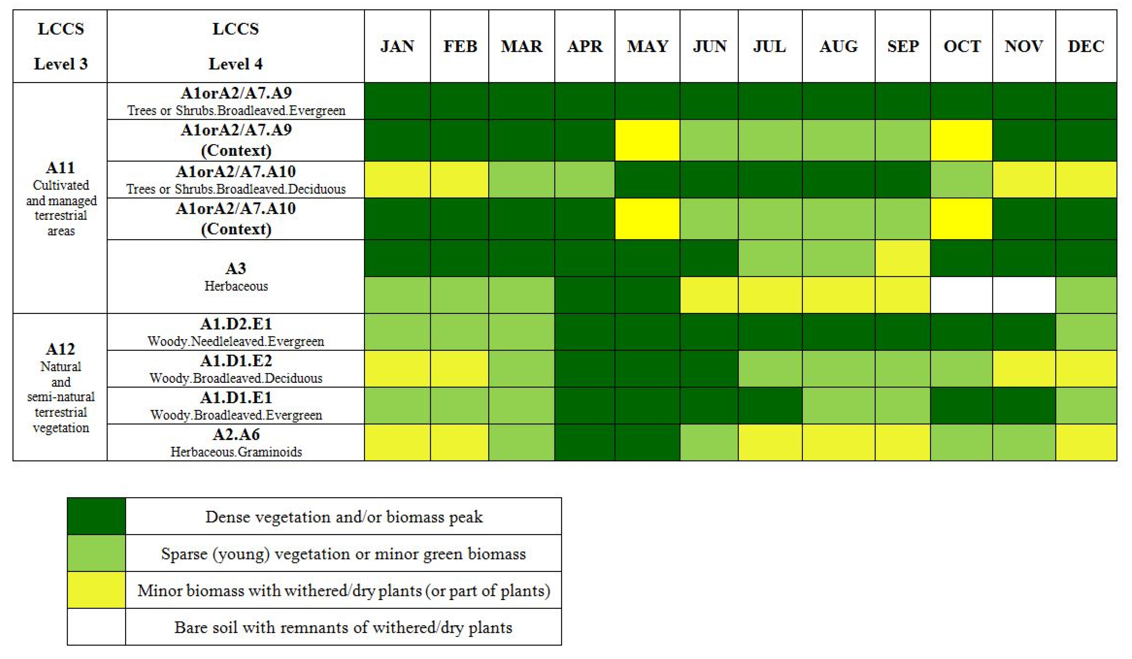
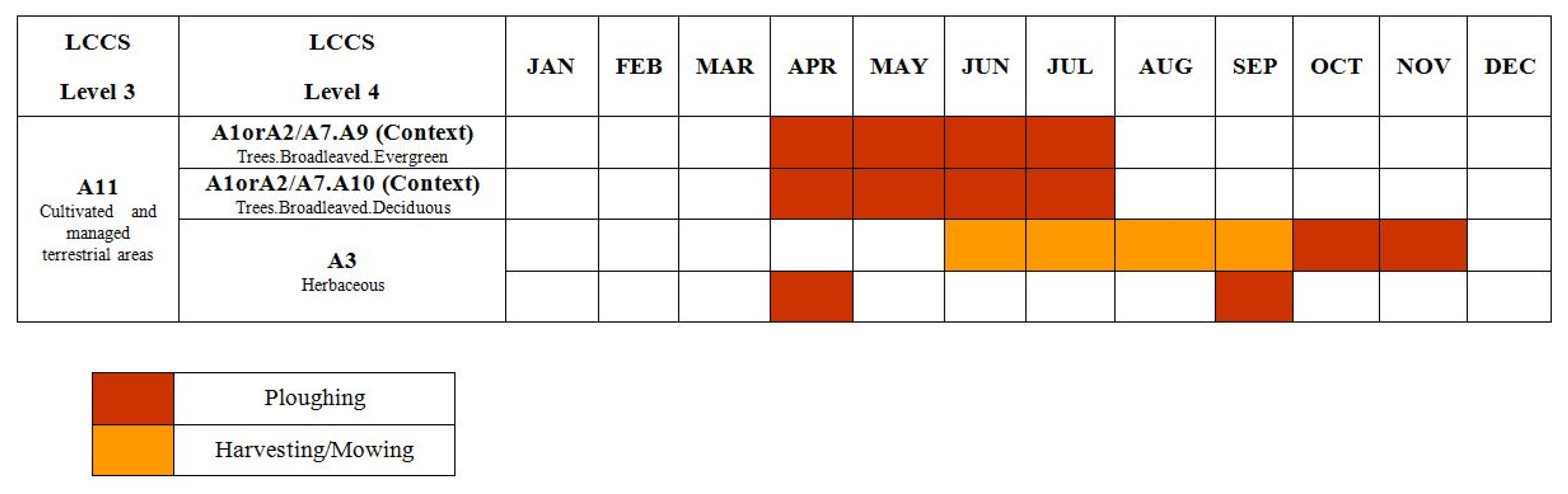
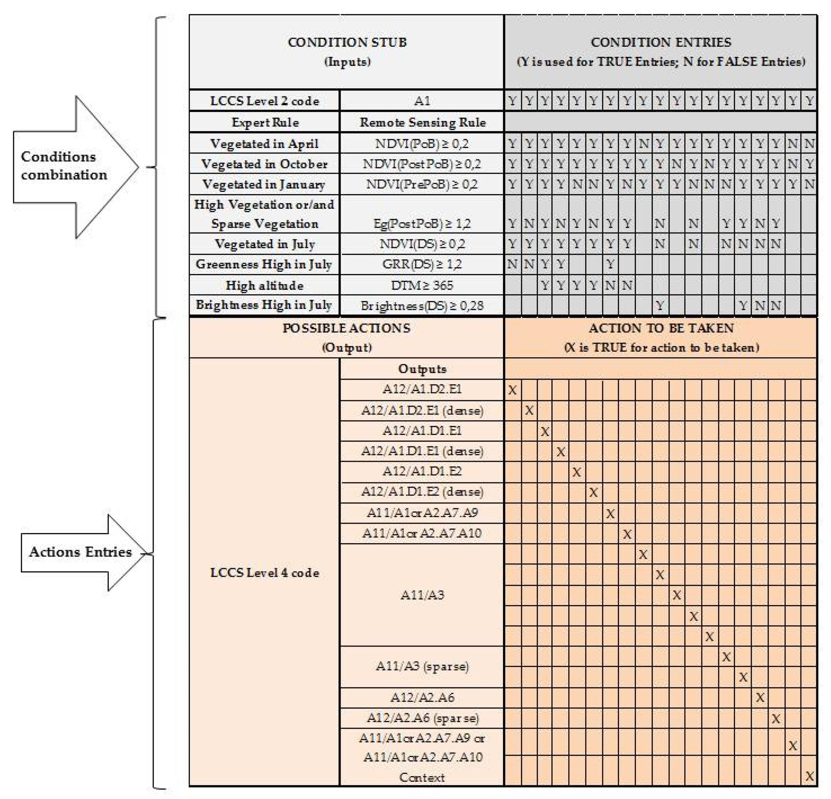
3.2. Expert Knowledge Elicitation

In this work, LCCS classifiers have been implemented in the classification algorithm developed for satellite image analysis along with expert knowledge rules from ecologists related to class description. Such description includes information about:

(1)

Core and context class components. In VHR images, classes can appear to be composed of individually detectable core elements and other surrounding elements constituting the context. As an example, an olive grove field is composed by olive trees, as class core elements, surrounded by bare soil, grassland or emerging rocks as context background [66,67].

(2)

Class phenology. Vegetated class discrimination depends on different period of peak of biomass and plant development. Agricultural class discrimination is based on periodicity of agricultural practices (i.e., ploughing, harvesting/mowing). Aquatic class discrimination requires water seasonality information [46].

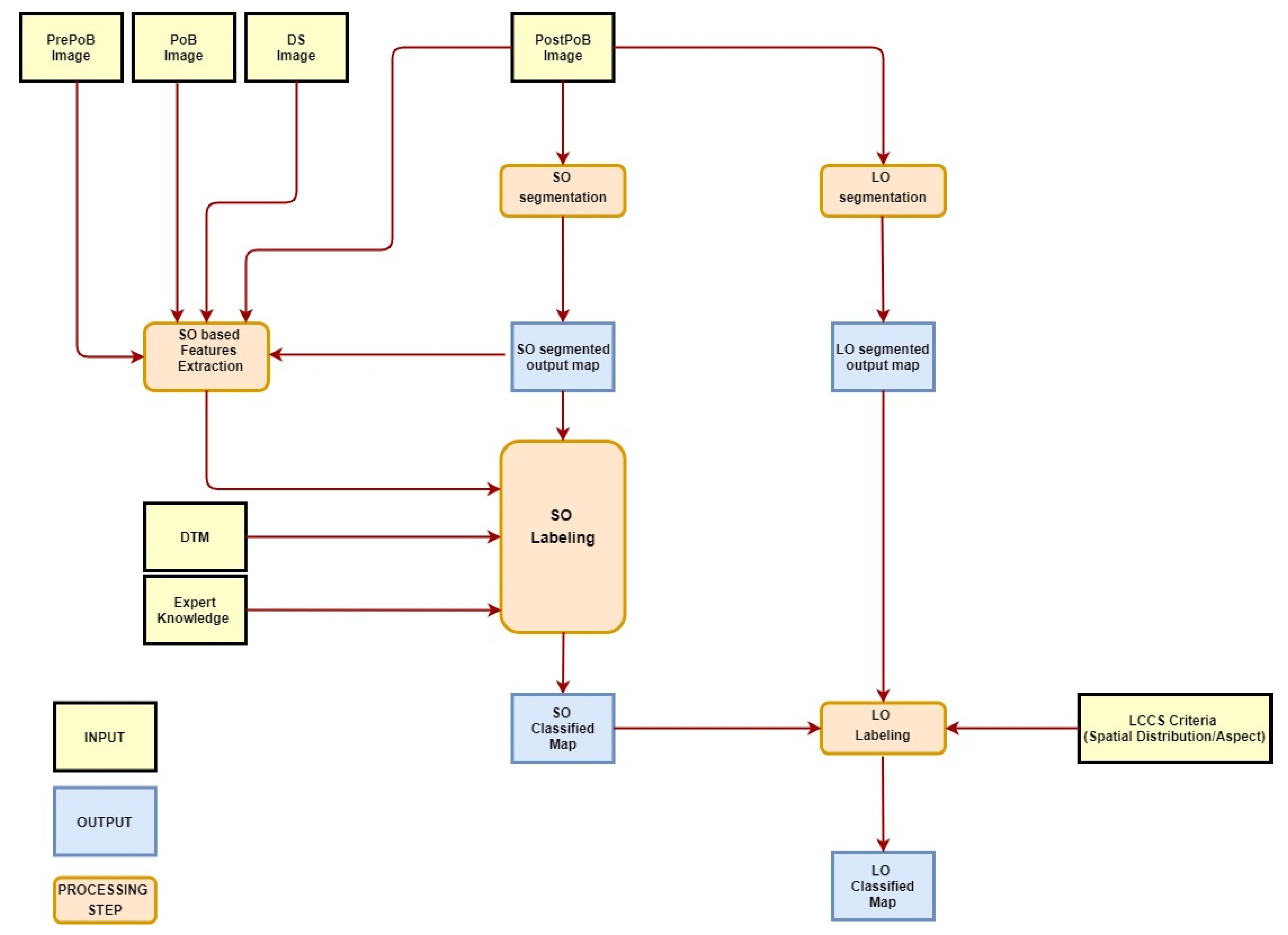
Expert knowledge exploitation depends on the implementation of an if-then rules set. Phenology and agricultural practices information can contribute to the selection of the most suitable multi-seasonal EO images, whereas core and context class description can support the selection of specific spectral, morphological, contextual and topological features and indices useful for target classes discrimination [68,69,70].

The list of expected LC classes in the scene are reported in

Table 3. List of small-object (SO) land cover (LC) classes in LCCS taxonomy in Murgia Alta site.

LCCS Level 4 Code	Class Description
A11/A1orA2.A7.A9	Cultivated and Managed terrestrial Areas/Trees or Shrubs.Broadleaved.Evergreen
A11/A1orA2.A7.A10	Cultivated and Managed terrestrial Areas/Trees or Shrubs.Broadleaved.Deciduous
A11/A3	Cultivated and Managed terrestrial Areas/Herbaceous
A12/A1.D2.E1	Natural and semi-natural terrestrial vegetation/Woody.Needleleaved.Evergreen
A12/A1.D1.E2	Natural and semi-natural terrestrial vegetation/Woody.Broadleaved.Deciduous
A12/A1.D1.E1	Natural and semi-natural terrestrial vegetation/Woody.Broadleaved.Evergreen
A12/A2.A6	Natural and semi-natural terrestrial vegetation/Herbaceous.Graminoids
B28/B27	Natural or Artificial waterbodies
B15	Artificial surfaces
B16	Bare Soil
Bare or vegetated context	Context of either class A11/A1orA2/A7.A9 or class A11/A1orA2/A7.A10

.

For Murgia Alta site, the information provided by ecologists to describe the classes (Table 3) is represented in Figure 2 and Figure 3. The former summarizes the phenology of vegetated classes, the latter represents the agricultural practices of cultivated vegetation. Such a scheme can be modified and adapted to any site.

3.3. The Algorithm

The classification procedure is composed by (a) the segmentation module and (b) the classification module, which can yield LC classification up to LCCS Level 4. Figure 4 shows the classification procedure flowchart.

Among the eight Worldview-2 bands available, only the Red, Green, Blue and NIR1 ones were intentionally considered as input to the system, for each date. The four bands were selected to offer a data processing methodology that may be applied also to other existing VHR data, such as the ones collected either on board of UAV and airplane platforms or from previous missions (e.g., Quickbird, Geoeye, IKONOS). The methodology could be applied to past and future data for change detection.

The PoB image (Table 1) resulted very useful for the discrimination of vegetated areas. The PrePoB image was mainly used for the disambiguation of evergreen and winter—deciduous woody classes (Figure 1a). The PostPoB image was mainly used for the identification of herbaceous graminoids cultivated classes (Figure 1b). The DS image was used for the disambiguation between herbaceous and woody classes. The latter was the only exhibiting a photosynthetic activity during the summer season (Figure 1c).

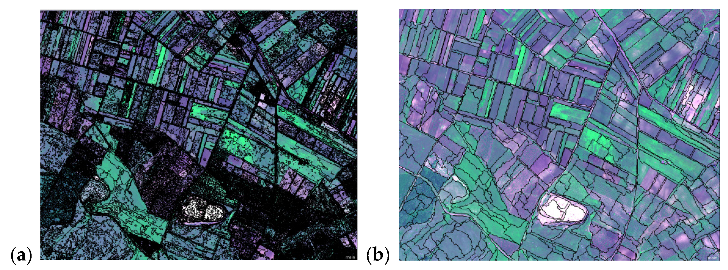
3.3.1. SO and LO Image Segmentation

In the present study, two different scales, i.e., the small object (SO) and the Large Object (LO) ones, were selected to segment VHR input imagery into landscape elements [71]. The two segmentation scales were carried out independently within an eCognition 8.0 framework [72].

To detect both SO and LO, only the spectral features of a single-date image were used, i.e., the October PostPoB image (R-G-B-Nir1 bands). This choice was based on the analysis of class separability values, with focus on the target class, i.e., grasslands. The Jeffreys–Matusita distance (JM) was used as separability indicator. As discussed by Hao et al., 2015 [73], previous research had shown that JM distance can provide a more accurate separability indicator than other distance measures, such as Euclidean distance or divergence. In particular, the multiclass extension of Jeffreys–Matusita distance, computed according to [74] for measuring the separability of grasslands with respect to other classes was considered to evaluate the best input images for segmentation. The analysis was carried out on both each single date and the whole multi-temporal dataset. The values of JM obtained were 2.2 for the PostPoB image, 2.0 for DS image, 1.6 for PrePoB image and 1.4 for PoB image. The value obtained for the whole multi-temporal data set was quite comparable (i.e., 2.3) with the one from PostPoB image (i.e., 2.2). Thus, we chose to use the PostPoB image only in the segmentation step for feature reduction purposes. This choice reduced the computational time of VHR image processing.

In addition, the PostPoB image appeared to better evidence not only the spectral differences between natural and agricultural herbaceous classes but also the contrast between tree crowns and their herbaceous context. Spectral band values were used for both SO and LO segmentation. For LO segmentation only, the 1st order entropy textural feature was added to discriminate high vegetation from low vegetation [75].

The SO scale was aimed at detecting all small elements in the scene (e.g., tree crowns) (Figure 5a) characterized by spectral homogeneity. For SOs identification, the eCognition spectral differences algorithm was applied. This algorithm merges neighbor pixels that fall within a user-defined maximum spectral difference. The spectral difference between adjacent pixels is calculated by considering their spectral values in the R-G-B-Nir1 bands of the PostPoB image [76]. In our study, the maximum spectral difference was set to 0.015 by trial and error. The main criteria used for such trial-error process was to recognize some of the finest elements (e.g., tree crowns) of the landscape, without over-segmenting the scene. Thus, visual interpretation of the different output segmented scenes addressed the parameter selection.

The LO scale was aimed at identifying landscape macro-structure classes (e.g., agricultural fields, olive groves) (Figure 5b). For LO identification, the multi-resolution image segmentation algorithm was used, since it can handle both spectral and context-sensitive features. This algorithm requires the definition of the following parameters: scale, shape or color heterogeneity, compactness or smoothness and weight of each spectral band [72]. Shape is complementary to color heterogeneity, whereas compactness is complementary to smoothness heterogeneity [77]. Thus, the eCognition algorithm used requires the setting of four independent parameters, namely scale factor, shape, compactness and weight of each spectral band. The first parameter controls the size of image objects [35]; the second quantifies the weight assigned to the object shape with respect to its spectral property, i.e., color; the third controls the balance between the object shape and its edge length [35].

In our study, the optimal segmentation parameters were selected through a supervised iterative process by tuning these parameters [35,36]. The optimal values found were: 5 for scale, 0.1 for shape and 0.1 for compactness, respectively. In addition, all the bands used in segmentation were equally weighted.

3.3.2. SO Classification

On the previous stage, each image segment identified can be considered a unit of analysis for which a number of attributes, including spectral response, texture, shape and location, can be extracted and used for classification. Specifically, every SO found in the image was labeled through LCCS classifiers related to Life Form, Leaf phenology and Leaf Type (Section 3.3.2).

To identify Level 1 and Level 2 LCCS classes, all the objects found in the SO map were classified by exploiting spectral indices only. Many indices were tested [44], the ones selected are summarized in

Table 4. Spectral indices used for LCCS classification.

Spectral Indices	Formula
Normalized Difference Vegetation Index (NDVI)	$\frac{{\rho }_{NIR}-{\rho }_{RED}}{{\rho }_{NIR}+{\rho }_{RED}}$
Green/Red Ratio (GRR)	$\frac{{\rho }_{GREEN}}{{\rho }_{RED}}$
Blue/NIR Ratio (BNR)	$\frac{{\rho }_{BLUE}}{{\rho }_{NIR}}$
Brightness	$\frac{{\rho }_{BLUE}+{\rho }_{GREEN}+{\rho }_{RED}+{\rho }_{NIR}}{4}$

. In the Table 4, ρ represents the TOA reflectance calculated as mean value of the image pixels inside each SO. The indices were extracted from the full set of multi-seasonal WV-2 images available.

Specifically, the Green/Red Ratio (GRR) [78] was used as a proxy for describing the photosynthetic status of vegetated classes [79]. Blue/NIR Ratio (BNR) performs well in discriminating water covered pixels [80]. The Brightness index was proven to be effective in identifying non-vegetated areas [44]. The indices reported were combined through a set of if-then rules grounded in remote sensing expert knowledge [65,81].

To obtain LCCS Level 1 classes, first the rules summarized in

Table 5. Rules used for Level 1 LCCS classification.

Spectral Rules	Logical Operators	Level 1 Temporary Classes	LCCS Level 1 Final Classes
NDVI(PoB) < 0.2	AND	Urban	Non-Vegetated (B)
BNR(PoB) ≥ 1.
Brightness(PoB) ≥ 0.15
NDVI(PoB) < 0.2	AND	Barren Land
NDVI(PrePoB) < 0.2
NDVI(PostPoB < 0.2
NDVI(DS) < 0.2
NDVI(PoB) ≥ 0.2	OR	Photosynthetic Vegetation	Vegetated (A)
NDVI(PrePoB) ≥ 0.2
NDVI(PostPoB) ≥ 0.2
NDVI(DS) ≥ 0.2
Photosynthetic Vegetation = TRUE	AND	Shadowed Vegetation
BNR(PrePoB) ≥ 1.15
BNR(PoB) < 1.
BNR(DS) < 1.

were applied. All image SOs resulted labelled into four temporary classes, i.e., Urban, Barren Land, Photosynthetic Vegetation and Shadowed Vegetation. At the end of the process, these classes were grouped into Vegetated (LCCS label A) and Non-Vegetated (LCCS label B).

Thereafter, the BNR index (

Table 6. Rules of the intermediate Level 2 classification.

Spectral Rules	Logical Operators	Level 2 Intermediate Classes
BNR(PoB) ≥ 1.	AND	Aquatic (2)
BNR(PrePoB) ≥ 1.
BNR(PostPoB) ≥ 1.
BNR(DS) ≥ 1.
Water = FALSE		Terrestrial (1)

) was exploited to label the same SOs as intermediate two classes, i.e., Terrestrial (1) and Aquatic (2).

After that, the final LCCS Level 2 label was assigned by considering all possible combinations of Level 1 final class labels (Table 5) and Level 2 intermediate labels (Table 6). As a result, four Level 2 image categories were obtained, namely, Vegetated Terrestrial (A1), Vegetated Aquatic (A2), Non-Vegetated Terrestrial (B1) and Non-Vegetated Aquatic (B2). The B15 (artificial areas) and B16 (bare areas) Level 3 classes coincided with the ones already identified as intermediate urban and barren land classes of Level 1, whereas B27/B28 (water bodies) class were derived from intermediate Level 2 aquatic class.

To discriminate Level 4 vegetated classes, the procedure identified a set of intermediate classes that were matched into the expected classes reported in Table 3. For this purpose, context-sensitive features were combined with DTM data and multi-temporal spectral indices.

Regarding spectral indices, logical operators were used to combine NDVI, GRR, Brightness to take into account the specific phenology of the vegetation classes and the agricultural practices of the study area. Specifically, the Brightness from the DS image was used to distinguish between perennial natural and cultivated herbaceous classes. This choice was based on the fact that in July graminoids cultivated fields appear bright due to mowing.

Concerning context-sensitive features, the texture first order entropy (occurrence measure) [82], from the green band of the PostPoB image, namely Eg(PostPoB), was used to discriminate herbaceous and woody vegetation. Texture was also found related to the sparseness of vegetation. The window size used to compute entropy was selected in order to match the scale of heterogeneity related to variations in vegetation height, distribution and structure.

The rule sets implemented for LCCS Level 4 mapping are reported in the decision table shown in Figure 5. Such table summarizes the different decisions to be taken according to different possible conditions. On the left upper part of the table, the possible input conditions are listed, one per each row. On the right upper part of the table, each column provides a possible combination of input conditions. The lower left part of Figure 5, indicates the various actions that can be taken, one per row. In the right part, each column reports whether that decision is taken for the specific combination of conditions [83]. In this study, the decision represents the label to be assigned to each input SO according to the combination of conditions reported in the upper part of the same Figure. As a result, for each input vegetated (A1) SO, an LCCS Level 4 class label was identified. The label was then assigned to each pixels of the SO object considered in the output map.

The rules from the ecologists are reported in the first column of Figure 6 (upper part), whereas the rules from the remote sensing experts reported in the second column of the same Figure (upper part) involve spectral rules and ancillary data, such as the DTM. The latter (line 9 of Figure 6) was introduced to support the discrimination of woody cultivated from other woody classes. In fact, cultivated woody trees (e.g., olive trees and orchards) are located at low elevation in Murgia Alta.

Complementary topological rules related to adjacency of barren land and herbaceous SOs to cultivated trees SOs were introduced to strengthen the final class decision but are not reported in the table. Contrary to the expert rule reported in Figure 3, some olive groves in April do not appear ploughed due to either new olive grove grassing techniques or to land abandonment.

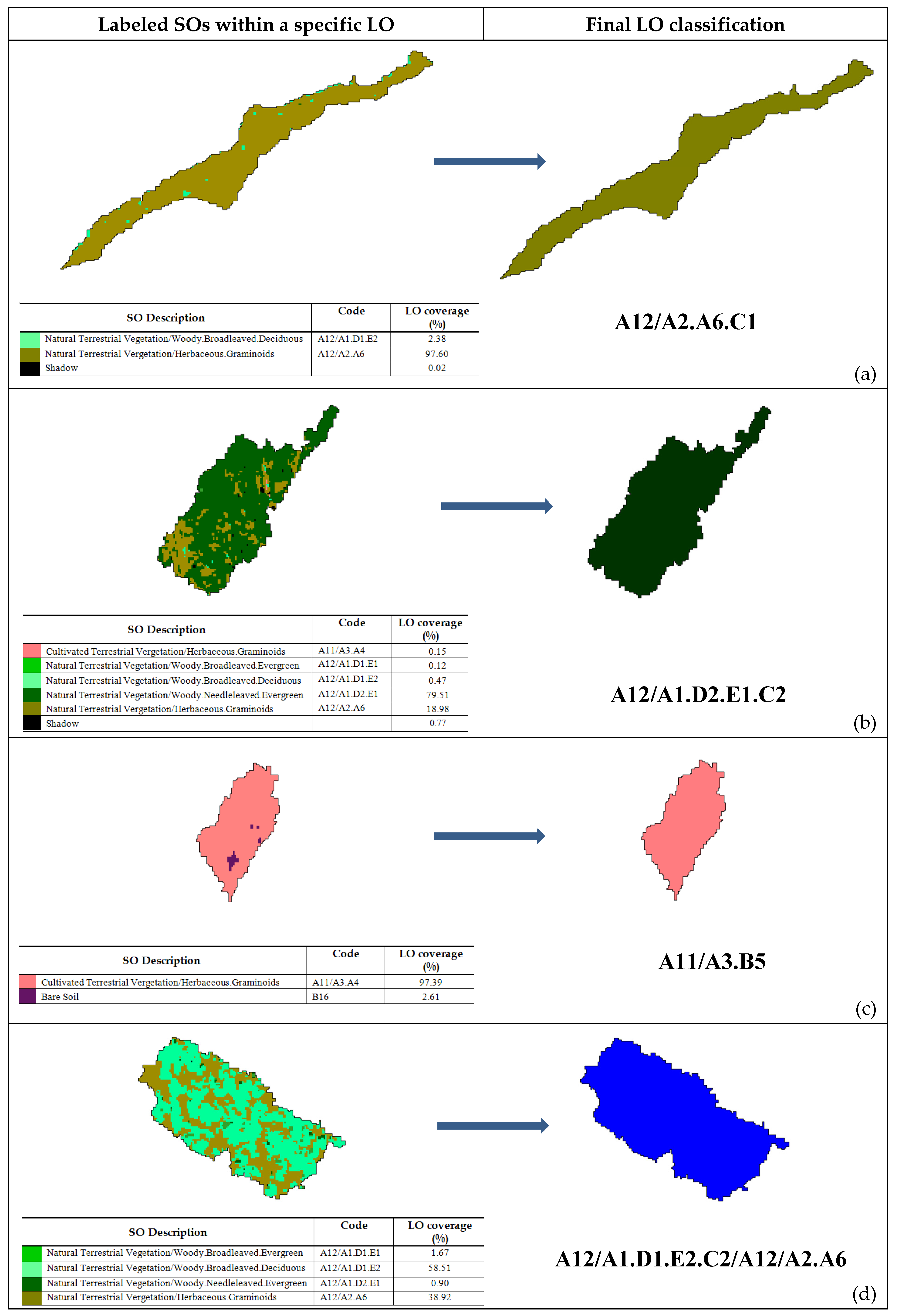
3.3.3. LO Classification

In the LO classification process, each segment was labeled according to LCCS rules based on the dominance criteria of SO classes within that LO. The dominance criteria were built upon a set of thresholds on the proportion of each SO class coverage included in the LO considered. The FAO-LCCS rules employed concerned only vegetated classes and involved Spatial Distribution and Spatial Aspect classifiers (Section 3.3.3), for natural vegetation and cultivated vegetation, respectively (Table 2).

According to LCCS definition, for natural and semi-natural vegetation classification, i.e., A12 classes, Spatial Distribution involves two classifiers: C1 for continuous and C2 for fragmented vegetation. These classifiers are based on the percentage of LO covered by the vegetation type considered, compared to other classes present in that LO. For Cultivated and Managed Terrestrial Areas classification (A11), LCCS Spatial Aspect classifiers (B5 for continuous, B6 for fragmented) definition draws on rules based on the percentage of LO covered by one cultivated class type compared to other land cover classes present in the same LO. When two or three different LC classes are found in a LO without any specific class dominance, the latter is labeled as Mixed Unit.

In our study, the following rules were implemented to automatically classify LOs:

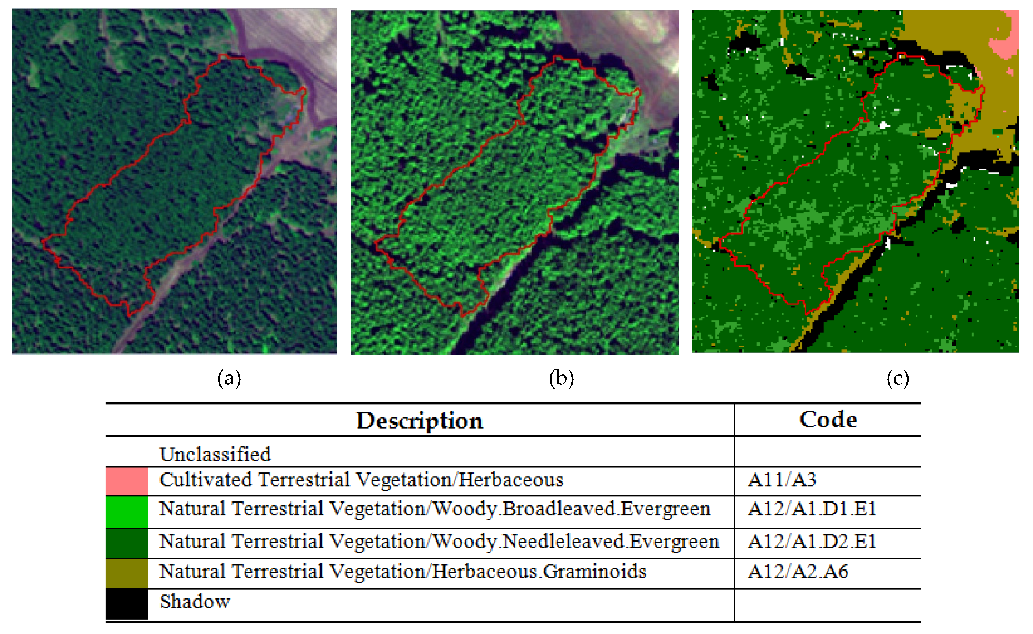
• When inside an LO, there was a class dominance, i.e., more than 80 percent of the pixels were labeled as a specific A12 class, the procedure assigned to the same label as the dominant class together with the C1 code (i.e., continuous spatial distribution) to the LO investigated (Figure 7a).
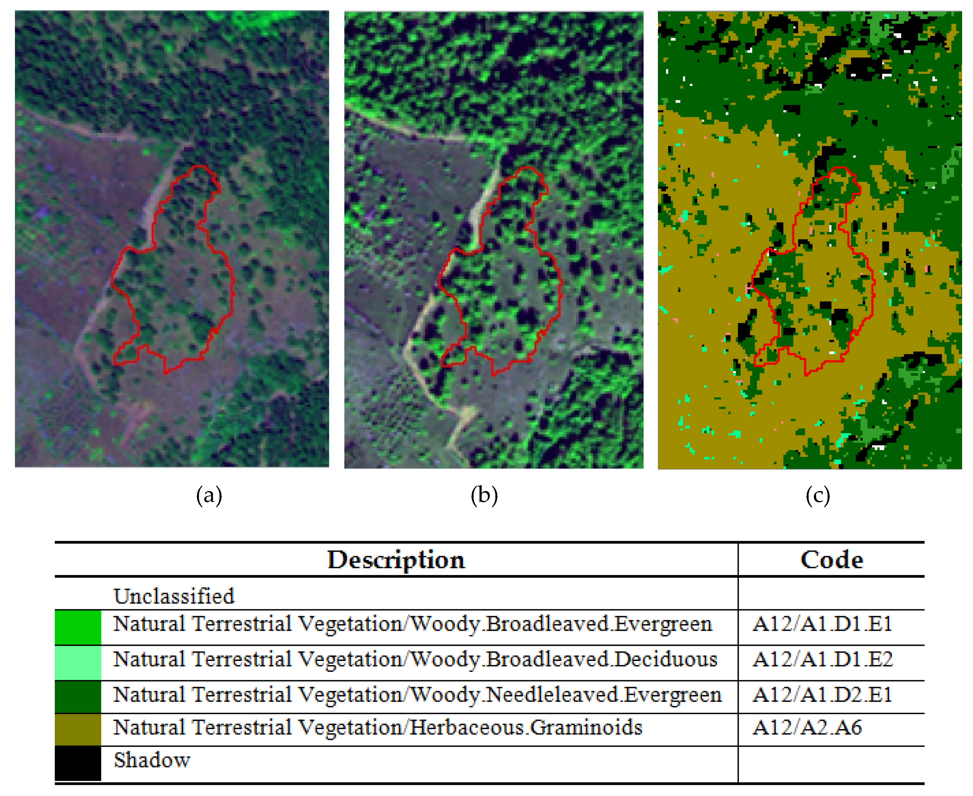
• When inside the LO, there was a class dominance, i.e., more than 50 percent but less than 80 of pixels labeled as a specific A12 class, and if neither of the other SO elements reached a cover exceeding 20 percent, the procedure assigned to the analyzed LO the same label as that of the dominant class together with the C2 code (Figure 7b).
• When more than 50 percent of cultivated SOs were found inside the LO analyzed, LO is to have A11 label with Continuous Spatial Aspect code (B5) (Figure 7c).
• When LO pixels belonging to a SO class X covered less than 80% but more than 50% of the LO extension, and a second SO class Y covered more than 20% but less than 50%, the LO was labelled as X/Y. This labelling indicates that both classes X and Y from SOs are present in the LO (co-presence), with class X covering the majority of the LO area. Specifically, when class X belonged to A12, the C2 code was added. When Y class belonged to class A11, code B6 (scattered clustered) was added to the Y class label [58] (Figure 7d)
• When the LO pixels met none of the above-mentioned rules, the LO was labeled as Mixed Unit.
• Due to the lack of specific rules for non-vegetated classes, in this study, we adopted the label “Mixed Units with artificial” to identify classes including both vegetated and artificial components. Instead when LOs included only SO of either B15 or B16 classes, the LO was labeled as single B15 or B16 unit.

3.4. Accuracy Assessment

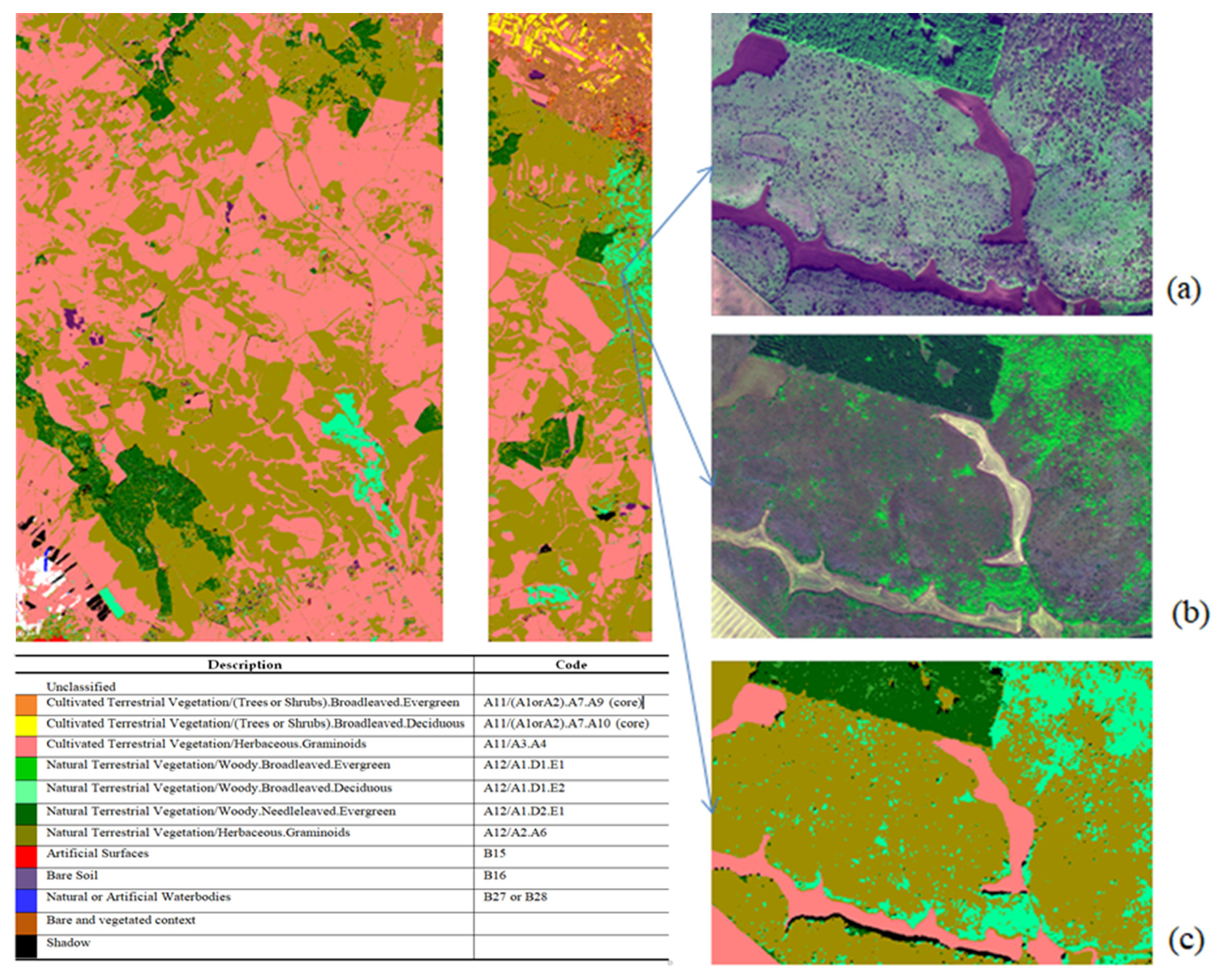
To identify sources of classification errors, in the automatic LCCS hierarchical classification scheme, accuracy assessment was carried out for each hierarchical classification step. Thus, the study provided the final SO output Confusion Matrix (CM) and four additional CMs, generated by Level 3 classes, LifeForm, Leaf type, Leaf phenology classifiers. Moreover, for LO validation, two additional CMs were produced. The first concerns the output of the Spatial Distribution or Spatial Aspect classifiers; the second concerns the Level 3 label of the co-dominant object (case (c) of Section 3.3.3).

The Overall (OA), the User’s (UA), the Producer’s (PA) accuracy values and F1-score were provided. In addition, the entropy-modulated accuracy (EMA) value [84] was included.

EMA formulation is based on the reference marginal vector entropy conditional to the classified marginal vector H(Ref|Class). Conditional entropy measures the information of the reference marginal vector, which may have been missed by the classified one. EMA is invariant to permutations in the CM columns and independent from the CM’s diagonal. This characteristic allows to evaluate classification accuracy without explicit matching between the reference and classified class labels, as in cases of non-square CMs.

In the present study, EMA was calculated as follows:

EMA = 1/e^H(Ref|Class).

(1)

Such formulation was introduced for normalizing EMA measurements to the percentage of correctly classified observations.

LO classification validation was performed by randomly selecting LO segments found on the output map. Such segments were labelled either by expert visual interpretation of the multi-temporal VHR data set or through in-field campaigns. Specifically, a total of 1586 objects were considered for LO reference data set in the validation process. This validation approach is commonly used for the accuracy assessment of LC maps obtained through GEOBIA [85,86].

4. Results

The investigation was carried out to assess the effectiveness of an object-oriented knowledge driven classifier of multi-temporal VHR images instantiated according to the FAO-LCCS hierarchical classification scheme into SO and LO output maps. This application has yielded encouraging results for LC mapping in Murgia Alta National Park and subsequent extraction of the relative natural grassland ecosystem layer.

4.1. SO Classification

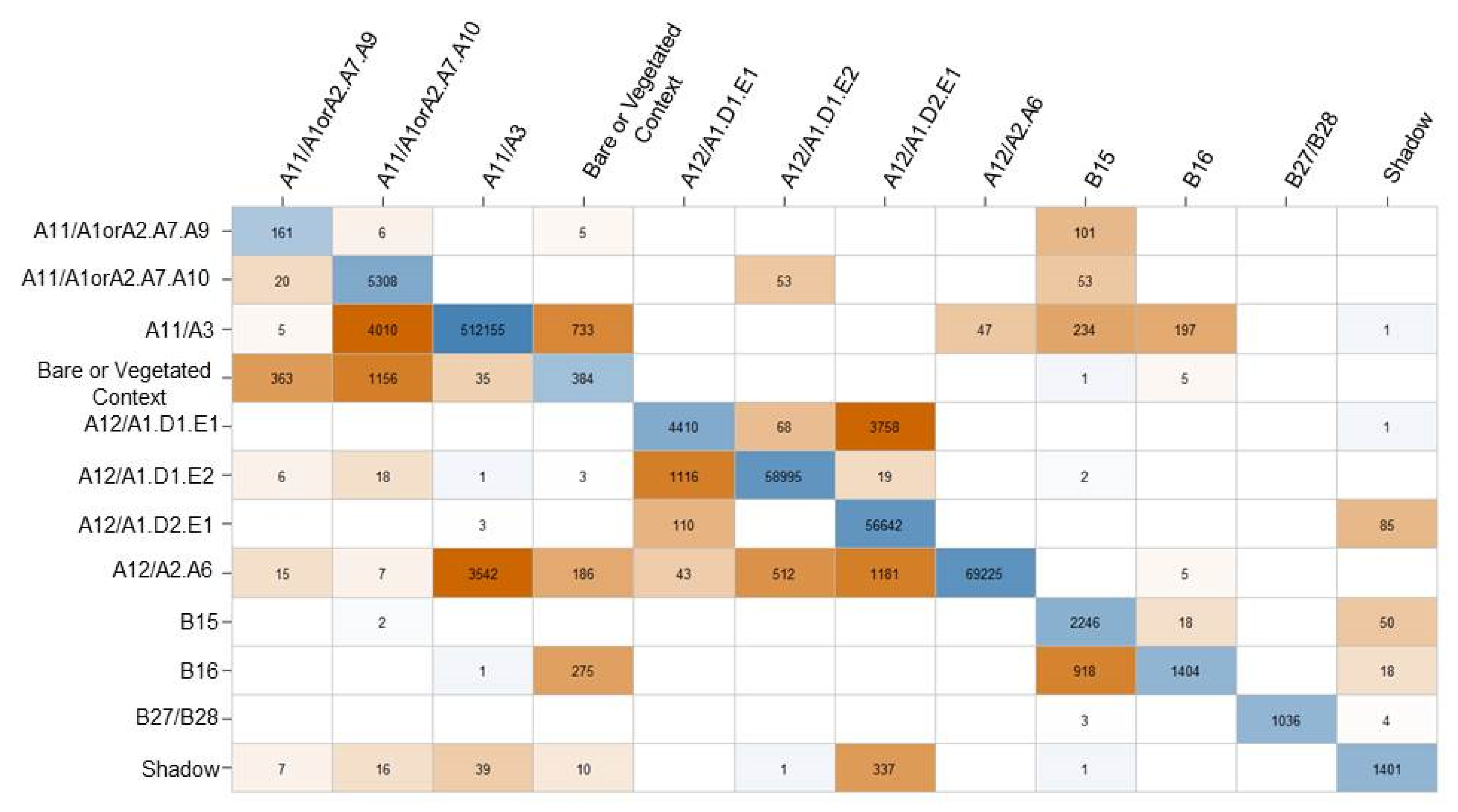
Some classes in VHR imagery correspond to core SO components surrounded by context SOs. For instance, an olive grove can include not only olive trees (core elements, A11/(A1orA2).A7.A9), which at the SO scale, can be individually observed, but also context components, such as herbaceous or barren land objects. The context components were labelled as bare or vegetated context in the list of SO output classes (Table 3).

Figure 8 reports the CM related to SO output classes. The OA value from the CM resulted quite high, i.e., 97.35%, with an error of 0.04%. The UA and PA percentage values and the F1-score obtained for each class of the SO map are shown in

Table 7. SO Accuracy assessments results at Level 4.

Classes	UA%	PA%	F1-Score
A11/A1orA2.A7.A9 Cultivated Terrestrial Vegetation/(Trees or Shrubs).Broadleaved.Evergreen	59.0	27.9	37.9
A11/A1orA2.A7.A10 Cultivated Terrestrial Vegetation/(Trees or Shrubs).Broadleaved.Deciduous	97.7	50.4	66.5
A11/A3 Cultivated Terrestrial Vegetation/Herbaceous.Graminoids	99.	99.3	99.1
Bare or Vegetated Context	19.7	24.1	21.7
A12/A1.D1.E1 Natural Terrestrial Vegetation/Woody.Broadleaved.Evergreen	53.5	77.6	63.4
A12/A1.D1.E2 Natural Terrestrial Vegetation/Woody.Broadleaved.Deciduous	98.1	98.9	98.5
A12/A1.D2.E1 Natural Terrestrial Vegetation/Woody.Needleleaved.Evergreen	99.69	91.4	95.4
A12/A2.A6 Natural Terrestrial Vegetation/Herbaceous.Graminoids	92.6	99.9	96.1
B15 Artificial Surfaces	97.0	63.1	76.5
B16 Bare Soil	53.7	86.2	66.1
B27/B28 Natural or Artificial Waterbodies	99.3	100	99.7
Shadow	77.3	89.1	83.1

.

The results reported indicate that:

(a)

The rule sets implemented perform well to discriminate natural vegetation classes. In particular, with exception to A12/A1.D1.E1 (natural/woody.broadleaved.evergreen), the F1-score resulted greater than or equal to 90%.

(b)

The rules appear to be less effective for cultivated woody classes discrimination. The F1-score values of A11/A1orA2.A7.A9 (cultivated/trees or shrubs.broadleaved.evergreen) and A11/A1orA2.A7.A10 (cultivated/trees or shrubs.broadleaved.deciduous) resulted to be 37.9 and 66.5, respectively.

(c)

The CM indicates that cultivated and natural woody classes were effectively discriminated, based on DTM measurements, whereas core and context components of the cultivated classes were less distinguishable. This might be due to both ortho-rectification issues as well as to different tree crown cover.

(d)

The F1-score of A12/A2.A6 (natural/herbaceous.graminoids) resulted quite high, i.e., 96.1%. However, the CM evidenced some misclassifications between such class and A11/A3 (cultivated/ herbaceous). On the contrary, A12/A2.A6 (natural herbaceous.graminoids) resulted to be well discriminated from all natural woody classes.

Figure 9 shows close-ups of Murgia Alta. The Figure 9a,b show that natural and semi-natural grasslands have complex and highly fragmented patterns. Such fragmentation is due to both the interference of cultivated herbaceous vegetation within grassland patches and the encroachment by woody broadleaved deciduous vegetation.

Hierarchical Accuracy Assessment

Table 8. OA and entropy-modulated accuracy (EMA) values for each SO hierarchical classification phase. P is the percentage of the reference data used in each specific confusion matrix (CM).

		OA%	EMA%	P%
Level 3	Dichotomous phase	99.22	96.31	99.57
Level 4	Life form classifier	98.99	94.66	98.84
	Leaf Type classifier	97.02	88.95	17.83
	Leaf Phenology classifier	99.05	95.25	17.83
Overall Output map	SO	97.35	89.75	100

reports the classification accuracies obtained from CMs for the different LCCS classifiers (levels) together with the final SO map overall accuracy. The percentage of the reference data (P) used for validation purposes is reported in the last column of Table 8. The full set of reference class data set, i.e., p = 100%, was used only to obtain the OA and EMA values of the final output map, whereas for intermediate hierarchical classification layers (i.e., Level 3, Level 4), p values were lower due to the fact that the classifiers used (e.g., Life Form) involve only some of the reference data.

LCCS Life Form classifier involves the discrimination of woody/herbaceous classes while Leaf Type concerns the discrimination between broadleaved/needleleaved classes of only woody vegetation objects. The choice to consider only the latter classes was motivated by the fact that in Murgia Alta, herbaceous vegetation mainly consists of graminoids classes. In view of this, no discrimination rule was adopted to distinguish between graminoids and forbs Leaf Type. Leaf Phenology allows to discriminate between evergreen/deciduous. In the area investigated, herbaceous vegetation includes annual and mixed phenology, thus Leaf Phenology was not considered for herbaceous vegetation.

The OA values reported in Table 8, evidence that the algorithm yielded a lower accuracy in identifying different Leaf Types compared to other classifiers considered (i.e, Life Form and Leaf Phenology). The lower accuracy reported may have been due to the fact that only NIR reflectance data were exploited to discriminate different Leaf Types.

The good performance obtained at the LifeForm classifier level (98.99%) confirms that the entropy measure is a suitable texture feature for the discrimination of herbaceous and woody vegetation (Supplementary Materials for further results).

The same Table reports also the EMA values. As can be observed, EMA yielded slightly lower values than the ones obtained through the classic accuracy approach.

With the exception of the Leaf Type classifier, the EMA values obtained from each layer considered resulted higher than the value obtained at the end of the SO classification procedure (89.75%). The latter finding appears to confirm the weakness of the rules applied at Leaf Type level.

It can be noted that the values reported in Table 8 show the EMA values have similar fluctuations as the ones in OA values.

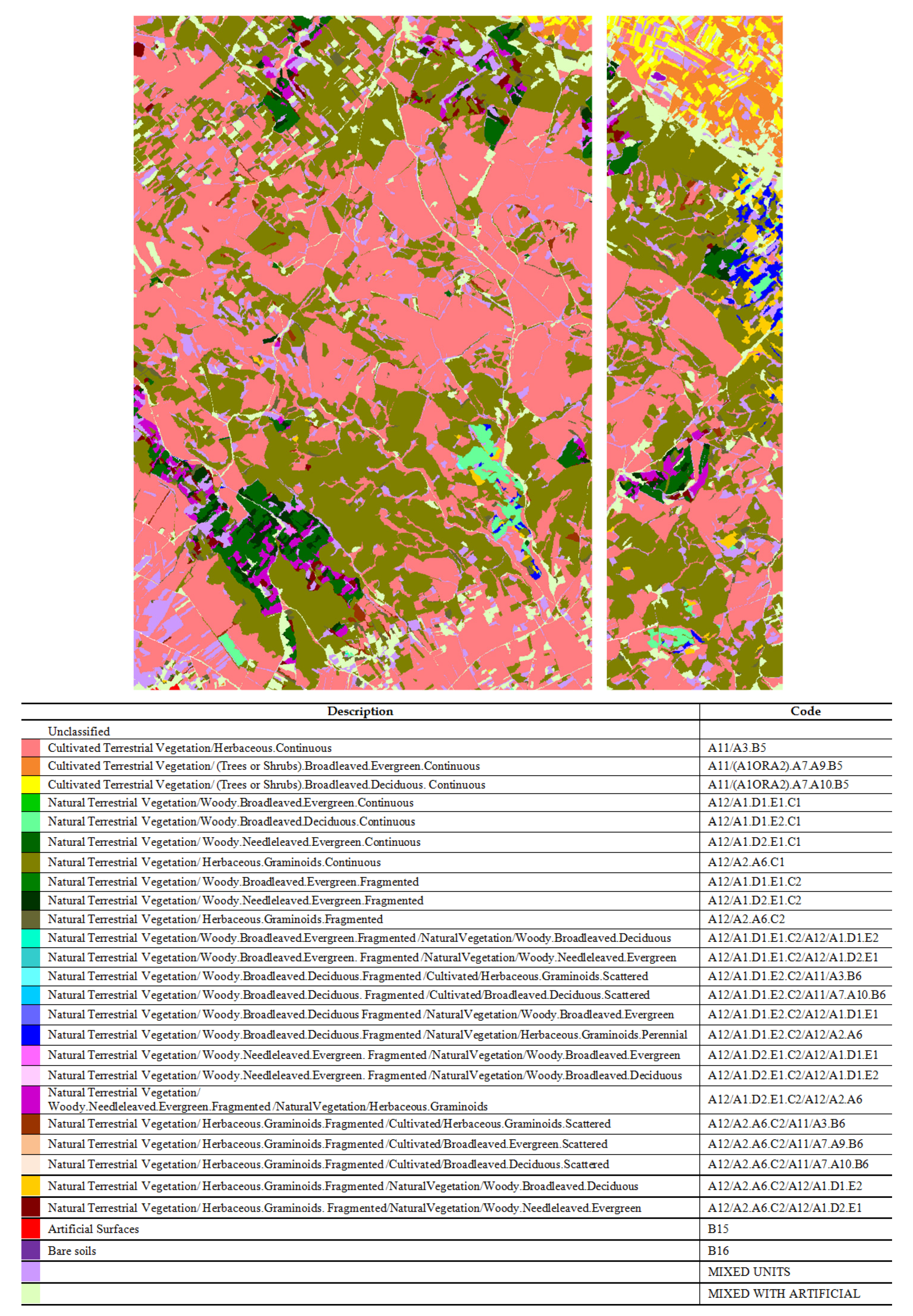
4.2. LO Classification

Table 9. List of the LO classes found by automatic classifiers and visual interpretation.

Single Units	Continuous Spatial Distribution	A12/A2A6C1
		A12/A1D2E1C1
		A12/A1D1E1C1
		A12/A1D1E2C1
	Continuous Spatial Aspect	A11/A3B5
		A11/(A1ORA2)A7A9B5
		A11/(A1ORA2)A7A10B5
	Fragmented Spatial Distribution	A12/A1D1E1C2 +
		A12/A1D2E1C2
		A12/A2A6C2
		A12/A1D1E2C2 *
		B15
		B16
Mixed Units	Continuous Spatial Distribution	A12/A2A6C2/A12/A1D1E2
		A12/A2A6C2/A12/A1D2E1
		A12/A1D2E1C2/A12/A2A6
		A12/A1D1E1C2/A12/A1D1E2
		A12/A1D1E1C2/A12/A1D2E1 +
		A12/A1D1E2C2/A12/A1D1E1
		A12/A1D2E1C2/A12/A1D1E1 +
		A12/A1D1E2C2/A12/A2A6
		A12/A1D2E1C2/A12/A1D1E2
	Continuous Spatial Distribution/Scattered Clustered	A12/A2A6C2/A11/A7A10B6 +
		A12/A2A6C2/A11/A3.B6
		A12/A1D1E2C2/A11/A7A10B6
		A12/A2A6C2/A11/A7A9B6
		A12/A1D1E2C2/A11/A3B6 +
		A12/A1D2E1C2/A11/A7A9B6 *
		Mixed Units
		Mixed Units with Artificial

reports the list of LO output classes, whereas Figure 10 shows the LO classified map.

It should be noted that the labels in Table 9, bearing an asterisk (*) represent vegetation classes that, although not found by the proposed knowledge-based classifier, were identified by visual image interpretation of the input images. Classes bearing a plus symbol ⁽⁺⁾ are instead those LO classes that, although recognized by the classification algorithm, were not identified by visual interpretation. In fact, LO labelled A12/A1D1E2C2 (natural/woody broadleaved evergreen) by visual interpretation were never detected by the automatic classifier. The latter was able to identify, instead, objects labelled as A12/A1D1E1C2 (natural/woody broadleaved deciduous). This finding might be due to co-registration issues since young trees’ crown may not cover more than 1–2 pixels.

Due to the inhomogeneity between classes obtained through VHR classification and those representing ground truth data, the CM results are rectangular. Therefore, in order to estimate the LO map accuracy, the CM was transformed in a square matrix [87]. Where a systematic mismatch occurred between automatic (i.e., classified) and visual (i.e., reference) evaluation of dominance criteria, the EMA measurement was more effective for evaluating LO classification accuracy.

Table 10. Overall accuracy (OA) and EMA values for LO hierarchical classification. P is the percentage of the reference data used in each specific CM.

		OA%	EMA%	P%
Level 3	Dichotomous	87.52	74.51	100
Level 4 Classifiers	Life form	93.34	80.21	92.81
	Leaf Type	95.57	93.65	41.30
	Leaf Phenology	89.31	80.16	41.30
	Spatial Distribution	91.78	82.57	92.81
	Secondary	98.06	98.90	64.94
Level 4 Output map	LO	75.09	63.02	100

reports both the final LO map OA (75.09%) and EMA (63.02%) values obtained for each LO hierarchical classification layer. The OA and EMA values showed a similar trend. The values reported for the dichotomous layer were lower than the ones obtained for all the other layers. This may be due to the classifier adoption of mixed units to meet the lack of specific rules to manage all possible class combinations in the LCCS taxonomy. The shortcoming evidenced may have generated misclassifications and overestimation of generic Mixed Units with a negative impact on the OA value.

The data presented in Table 10 indicate a rather good performance obtained for Life Forms, Leaf Type, Leaf Phenology and spatial distribution of the dominant class. The OA and EMA values from both single layers and the final map appeared to be lower than those reported in the validation of SO (Table 8). The following should be noted:

• The classifier parameter selection by a trial and error procedure can generate an LO segmentation inadequate to represent the structure of landscape patches. As a result, non-existing LO classes can occur, such as the ones indicated with (⁺) in Table 9.
• LO map accuracy can be influenced by the SO map accuracy as well as by the lack of specific FAO-LCCS rules for non-vegetated classes.

5. Discussion

The results reported in the present study seem to encourage the use of the knowledge-driven object-based classification system validated through the use of both accuracy and EMA values for the mapping of natural grassland ecosystems. The main novelty of the proposed methodology is rooted in the implementation of the hierarchical classification scheme of the Food and Agricultural Organization (FAO) Land Cover Classification System (LCCS) taxonomy.

To the best of our knowledge, FAO-LCCS taxonomy has been used extensively to label ground reference class samples collected by in-field campaigns. Except for a recent paper [44], the hierarchical set of rules of such taxonomy has not been used in GEOBIA classifiers. In particular, the novelty of this study includes the way SO were used to label LO, according to specific FAO-LCCS spatial distribution and spatial aspect properties of natural and cultivated classes adopted. As a specific advancement of previous work in [44], such properties were adopted to evaluate the dominance of SOs within each LO.

In addition, the proposed approach guarantees consistency between the rules adopted by the GEOBIA classifier and the ones used to collect reference-validation samples during in-field campaigns [61]. Thus, this coherence facilitates the validation of the output maps.

The knowledge driven approach proposed is closer to the way end-users conceptualize their domain expertise; hence, it contributes to deepen the gap between image processing scientists and end-users. As evidenced in [40], working with symbolic knowledge enhances knowledge management. It also facilitates collaborative and interdisciplinary research by connecting concepts from different scientific domains (in ecology, agriculture, geo-health etc.) This paper offers a contribution in such direction.

5.1. SO Results Discussion

The proposed method seems to perform well in the classification of natural vegetation. In particular, the results obtained for A12/A2.A6 (natural/herbaceous.graminoids) classification, i.e., OA values 97.35% and 92.6%, 99.9% and 96.1% of UA, PA and F1-score, respectively (Table 7), encourage the application of SO classification method for the monitoring of grassland and grassland encroachment at VHR. The less satisfactory performance obtained for A12/A1.D1.E1 (natural/woody.broadleaved.evergreen) classification can be explained in consideration of the fact that, in the study site, this class results highly fragmented due to their interspersion with broadleaved deciduous. The Hierarchical accuracy assessment shows that, at the level of LifeForms, the classes were well discriminated. This is due to the use of 1st order entropy to discriminate low and high vegetation. Such result is in agreement with the findings of previous studies [68,75].

As evident in the CM, problems cropped up in discriminating B15 and B16. The classification of these classes relies on the exploitation of the Brightness index. Since the Murgia Alta region is characterized by bright rocky outcrops as well as by bright soil containing grained rocks, B15 (artificial areas) may have been misclassified as B16 (bare soil).

The values obtained for the SO map resulted in OA equal to 97.35%, with error 0.04%, and in UA, PA and F1-score values for grasslands equal to 92.6%, 99.9% and 96.1%, respectively. Even though our results regard only one site, these values can be considered comparable or better than the values from previous pixel-based and object-based supervised approaches. For instance, Raab et al., 2018 [31], discriminated several grassland communities from RapidEye (5 m pixel size) imagery through a pixel-based RF supervised classifier and reported a mean OA of 80%. In their study, these authors used a dense data set including pre-spring, first spring, full-spring, early summer, midsummer late summer, early autumn, full autumn and late autumn images. Even though in their paper the authors used more detailed phenological information, the comparison between their results and ours suggests that, when analyzing VHR imagery, an object-based approach can provide better performance than a pixel-based approach.

Schuster et al., 2015 [11], assessed the suitability of a RapidEye time series (21 images) to identify several grassland species. The authors adopted a pixel-based, supervised data driven SVM classifier and obtained and OA of 90%, which cannot be directly compared to our results. In fact, their findings deal with the discrimination of more than one species of grasslands from VHR time series.

Melville et al., (2018) [30], used an object-based supervised RF classifier to analyze a single date Worldview-2 image for the classification of three grassland classes and other land cover types. In their study, they report an OA of 80%. This may have been due to the use of only one date; thus, the phenology of different vegetated classes cannot be adequately represented. For this reason, in our work, we have used multi-seasonal imagery, selected on the basis of prior phenology knowledge rules of the study classes.

Onojeghuo and Onojeghuo, (2017) [37] used an object-based SVM classifier to analyze satellite multispectral, airborne hyperspectral and LiDAR DTM data set for habitat mapping, including grasslands. In this study, the results showed a significant increase in classification accuracy when the DTM was combined with spectral information with a final OA of 89.8%. These findings confirm the utility of DTM in combination with spectral information for VHR data classification, as done also in our study to discriminate cultivated from natural woody vegetation.

Clerici et al., (2017) [36], integrated radar and visible-near infrared data set for object-based supervised classification. The data driven SVM algorithm produced the most accurate LCLU map, including grasslands class with an OA of 88.75%. The grasslands UA and PA obtained were 81.25% and 18–75%, which are significantly lower than the values obtained with our knowledge–driven classifier.

Xu et al., (2018) [27], focused on the classification of different grassland types from multi-temporal Landsat images, in combination with a 30-m DTM. The authors used both SVM and RF object-based classifier. The OBJA classifiers were able to differentiate different grassland types from multi-source data. The overall classification accuracy exceeded 90% using both classifiers, and the classification accuracy of the grassland types considered ranged from 61.64% to 98.71%. In agreement with our findings, Xu et al. evidenced that multi-temporal images and auxiliary data can improve grasslands classification.

A comparison between the results reported in the above-mentioned studies and the ones obtained in our study suggests that the hierarchical knowledge-driven object-based classifier can yield high OA values comparable with the ones obtained by both pixel- and object-based data-driven supervised classifiers. Unfortunately, it is not always easy to collect a large number of quality training samples due to limited time, access or interpretability constraints. A further complication is that if data quality is a concern, such as mislabeled data samples, then it may be necessary to select an algorithm that is less sensitive for such issues [35].

As recently evidenced in [40,41,88,89], knowledge-driven approaches based on enhanced computing capacities are gaining importance to analyze big Earth Observation data. The remote sensing community considers the development of knowledge-driven approaches to be one of the most important directions of their research. However, so far, little effort has been dedicated to formalizing, aggregating and sharing expert knowledge in remote sensing applications. Such knowledge could be used to develop ontologies.

Ontologies have the capacity to represent both symbolic and numeric knowledge, to reason based on cognitive semantics and to share knowledge on the interpretation of remote sensing images. This approach will generate new knowledge and services by integrating multiple source/domains information [90].

Gu et al., (2017) [42], used a hybrid approach to analyze a single date VHR ZY-3 image. In their work, first, a data driven LCCS hierarchical classification phase was carried out. Then, an ontology was used to relabel the objects. The ontology was based on the combination land cover classes obtained in the previous phase with various features selected by prior knowledge as well as with existing ontologies. In term of OA values, similar results were obtained with and without the ontology, i.e., 85.95% and 84.32%, respectively, whereas the specific grasslands UA improved from 78.26 to 85.37, after ontology exploitation. Such UA increase seems due to a better generalization capability. Compared to such results, our knowledge-driven approach provided both quite high values of OA (97.35%) and grassland PA (92.6%) values. This is mainly due not only to the use of multi-seasonal VHR images, but also to elicitation of phenology and agricultural practices rules.

It seems also worth noting that despite the complexity of the knowledge elicitation process required by our approach, the analysis of VHR images through the hierarchical classifier can represent better the heterogeneity of the grassland ecosystem and its dynamic.

5.2. LO Results Discussion

Following the SO classification, a LO classification was applied to represent the landscape heterogeneity through a multi-scale approach, which characterizes the GEOBIA paradigm [35]. When using different segmentation and labelling scales a crucial step is the merging of small-scale objects within the large-scale ones.

Watmough et al., (2017) [33], used segmentation scales ranging from the coarser to the finest and applied different features to each scale examined in order to provide both different classification layers and different output classes. Momeni et al., (2016) [34], applied three different segmentation scales without adopting any merging criteria. Zhang et al., (2014) [71], proposed a multi-scale segmentation with equispaced scales. The latter authors merge different scale objects when finding a complete overlap between the different layers. The findings discussed by them cannot be adequately compared with the ones obtained in the present study. In fact, in our study, we used the LCCS taxonomy dominance criteria (Section 3.3.3) to merge the vegetated objects found at different scales. As far as we know, such approach was not exploited in previous studies.

However, the results of the dominance criteria application may differ when automatically applied to image object analysis or when evaluated through image visual interpretation, or in-field campaigns. Our study tried to address this challenging validation issue in search for a possible explanation. By analyzing the results obtained, the following factors seem to influence our validation process. These factors include SO labelling and its impact on the SO classification accuracy, LO segmentation accuracy and the effectiveness of the LCCS dominance rules for the classification of LOs.

Specifically, the LO classification process can be hampered by errors in the labelling of vegetated SO objects corresponding to cultivated orchard and olive groves (Figure 8). These errors may be mainly caused by the presence of small tree crowns, which include only a small number of pixels. Due to geo-referencing error (order of one pixel), the leaf phenology classifier might fail in classifying SOs. This might be due to pixels spectral features that could correspond to different objects on the ground (e.g., tree crown, soil, shadow). As a consequence, SO dominance in the LO may be mistaken. In addition, classification of LOs including SO of both cultivated orchard and olive grove were labeled as mixed units, due to the lack of LCCs criteria for evaluating the dominance of cultivated classes.

Another source of error may be the segmentation scale adopted. The latter may have aggregated landscape elements that should have been labeled as distinct objects into single LOs.

Moreover, for woody natural vegetation classes, confusion between either C1 (continuous) and C2 (fragmented) labels or C2 with or without co-dominant component may occur. Furthermore, confusion in the dominance of grassland or woody components in the LO considered when both classes are co-present may occur.

Confusion in validation process may depend on the perception that the expert may have had of the class dominance when providing reference samples to be used for LO classification. Figure 11 can exemplify this event.

The LO evidenced by the red polygon in Figure 11 was labelled as A12/A1D2E1C2/A12/A2A6 (a coniferous forest fragmented by grassland) by the expert, but it was labelled as A12/A2A6C2/A12A1D2E1 (grassland with scattered trees) by the hierarchical classifier. The latter applied the dominance criteria to SO pixels found within the specific LO. All adjacent SOs belonging to other LOs perceived by the expert were not analyzed by the algorithm. This perception of the context may have guided the expert during the visual interpretation and labeling of the object.

An additional example is provided in Figure 12, where the LO (in red line) was labelled as A12/A1D2E1C1 by the expert and as A12/A1D2E1C2 by the hierarchical classifier. The incongruence may have been due to the presence of broadleaved SOs in the LO mixed with coniferous SO components detected by the classifier, but it is difficult to detect by expert visual image interpretation.

The collection of reference data can be time-consuming and sometimes impossible to perform. The methodology proposed in the present study offers the advantage of the knowledge-driven approach that can avoid the need of training data.

Even though instantiation of the expert rules may require a significant amount of time to elaborate the decision tree, the expert knowledge requires less extensive in field campaigns. Moreover, such campaigns are not required to be repeated through time.

6. Conclusions

In the present paper we applied a knowledge-based GEOBIA classifier for mapping grasslands ecosystems. As a novelty, the classification algorithm instantiates the hierarchical FAO-LCCS scheme by exploiting:

(1)

A multi-temporal approach to identify different phenological vegetation attributes, combined with expert-knowledge from ecologists. This approach yielded satisfactory results in the discrimination of perennial and annual vegetation.

(2)

VHR imagery to reveal the suitability of features (i.e., context–sensitive) obtained through this approach. Without requiring additional data sources (i.e., CHM), entropy proved reliable in discriminating between high (trees and shrubs) and low vegetation (herbaceous).

(3)

R, G, B and NIR bands and derived indices were sufficient to recognize different ground targets. The choice to use only these bands was in light of the fact that VHR satellite data are very costly, whereas drone-flights with VIS-NIR bands become more and more frequently used to collect VHR images of local areas. As confirmed by Jabbour et al. 2020 [91], due to the cost of satellite images with spatial resolution lower than 5 m, end-users seem to prefer drone based acquisition of such data for decision making at local level. Thus, the proposed methodology can be applied to VHR data from drones.

These considerations suggest that that VHR resolution multi-temporal imagery in a GEOBIA classification framework complemented with expert knowledge can be reliable for grasslands ecosystem mapping in the Mediterranean area. This area is characterized by small fields of interconnected and fragmented habitats and ecosystems difficult to monitor with high resolution sensors such as Landsat and Sentinel-2. Thus, GEOBIA data driven classifiers seem adequate for detecting the landscape matrix at VHR. Without training samples, the proposed approach can be applied to other grasslands areas once local agricultural practices and phenology rules are elicited.

Concerning phenology, a hybrid approach could be used to automatically extract phenology parameters (e.g., yearly mean, yearly standard deviation, min-max day of the bio-mass peak) from intra-annual time series of Sentinel-2 free data in any site. Subsequently, VHR image could be tasked. The usefulness of phenological metrics obtained through the exploitation Time Series of high-resolution data within a GEOBIA classification scheme is going to be the object of a coming investigation.

Even though the use of LCCS criteria for LO classification would need further investigation, and in spite of the limited area in our study, the results obtained appear encouraging compared to supervised classifiers in the literature. So far, little effort has been dedicated to formalizing, aggregating and sharing expert knowledge in remote sensing applications [32]. This paper provides a methodology that can contribute to support the transition from a data-centric to a knowledge-centric approach [92]. This transition is strongly encouraged by the Group of Earth Observation (GEO) in support to decision makers.

References

1. Maes, J.; Teller, A.; Erhard, M.; Liquete, C.; Braat, L.; Berry, P.; Egoh, B.; Puydarrieux, P.; Fiorina, C.; Santos, F.; et al. Mapping and Assessment of Ecosystems and Their Services. An Analytical Framework for Ecosystem Assessments under Action 5 of the EU Biodiversity Strategy to 2020; 1st Technical Report; Publications Office of the European Union: Luxembourg, 2013. [CrossRef]
2. Maes, J.; Teller, A.; Markus Erhard, M.; Murphy, P.; Paracchini, M.L.; Barredo, J.I.; Grizzetti, B.; Cardoso, A.; Somma, F.; Petersen, J.E.; et al. Mapping and Assessment of Ecosystems and Their Services (MAES). Indicators for Ecosystem Assessments under Action 5 of the EU Biodiversity Strategy to 2020; Second Technical Report (2014-080); Publications Office of the European Union: Luxembourg, 2014. [CrossRef]
3. Ali, I.; Cawkwell, F.; Dwyer, E.; Barrett, B.; Green, S. Satellite remote sensing of grasslands: From observation to management. J. Plant Ecol. 2016, 9, 649–671. [Google Scholar] [CrossRef] [Green Version]
4. Zhao, Y.; Liu, Z.; Wu, J. Grassland ecosystem services: A systematic review of research advances and future directions. Landsc. Ecol. 2020, 35, 793–814. [Google Scholar] [CrossRef]
5. Tilman, D.; Socolow, R.; Foley, J.; Hill, J.; Larson, E.; Lynd, L.; Pacala, S.; Reilly, J.; Searchinger, T.; Sommerville, C.; et al. Beneficial biofuels–The food, energy, and environment trilemma. Science 2009, 325, 270–271. [Google Scholar] [CrossRef] [PubMed] [Green Version]
6. Klimek, S.; Richter, A.; Hofmann, M.; Isselstein, J. Plant species richness and composition in managed grasslands: The relative importance of field management and environmental factors. Biol. Conserv. 2007, 134, 559–570. [Google Scholar] [CrossRef]
7. Sullivan, C.A.; Sheey Skeffington, M.; Gormally, M.J.; Finn, J.A. The ecological status of grasslands on lowland farmlands in western Ireland and implications for grassland classification and nature value assessment. Biol. Conserv. 2010, 143, 1529–1539. [Google Scholar] [CrossRef]
8. Wright, C.K.; Wimberley, M.C. Recent land use change in the Western Corn belt threatens grasslands and wetlands. Proc. Natl. Acad. Sci. USA 2013, 110, 4134–4139. [Google Scholar] [CrossRef] [Green Version]
9. Scholes, R.J.; Mace, G.M.; Turner, W.; Geller, G.N.; Jurgens, N.; Larigauderie, D.; Muchoney, B.A.; Walther, H.A. Toward a global biodiversity observing system. Science 2008, 321, 1044–1045. [Google Scholar] [CrossRef]
10. De Bello, F.; Lavorel, S.; Gerhold, P.; Reier, U.; Partel, M. A biodiversity monitoring framework for practical conservation of grasslands and shrublands. Biol. Conserv. 2010, 143, 9–17. [Google Scholar] [CrossRef]
11. Schuster, C.; Schmidt, T.; Conrad, C.; Kleinschmit, B.; Forster, M. Grassland habitat mapping by intra-annual time series analysis–Comparison of RapidEye and TerraSAR-X satellite data. Int. J. Appl. Earth Obs. Geoinf. 2015, 34, 25–34. [Google Scholar] [CrossRef]
12. Hill, M.J.; Ticehurst, C.J.; Lee, J.; Fellow, L.; Grunes, M.R.; Donald, G.E.; Henry, D. Integration of optical and radar classifications for mapping pasture type in Western Australia. IEEE Trans. Geosci. Remote Sens. 2005, 43, 1665–1681. [Google Scholar] [CrossRef]
13. Bock, M.; Xofis, P.; Mitchley, J.; Rossner, G.; Wissen, M. Object-oriented methods for habitat mapping at multiple scales–Case studies from Northern Germany and Wye Downs, UK. J. Nat. Conserv. 2005, 13, 75–89. [Google Scholar] [CrossRef]
14. Prishchepov, A.V.; Radeloff, V.C.; Dubinin, M.; Alcantara, C. The effect of Landsat ETM/ETM+ image acquisition dates on the detection of agricultural land abandonment in Eastern Europe. Remote Sens. Environ. 2012, 126, 195–209. [Google Scholar] [CrossRef]
15. Franke, J.; Keuck, V.; Siegert, F. Assessment of grassland use intensity by remote sensing to support conservation schemes. J. Nat. Conserv. 2012, 20, 125–134. [Google Scholar] [CrossRef]
16. Mehner, H.; Cutler, M.; Fairbaim, D.; Thompson, G. Remote sensing of upland vegetation: The potential of high spatial resolution satellite sensors. Glob. Ecol. Biogeogr. 2004, 13, 359–369. [Google Scholar] [CrossRef]
17. Schmidtlein, S.; Zimmermann, P.; Schupferling, R.; Weib, C. Mapping the floristic continuum: Ordination space position estimated from imaging spectroscopy. J. Veg. Sci. 2007, 18, 131–140. [Google Scholar] [CrossRef]
18. Schuster, C.; Ali, I.; Lohmann, P.; Frick, A.; Forster, M.; Kleinschmit, B. Towards detecting swath events in TerraSAR-X time series to establish Natura 2000 grassland habitat swath management as monitoring parameter. Remote Sens. 2011, 3, 1308–1322. [Google Scholar] [CrossRef] [Green Version]
19. Feilhauer, H.; Thonfeld, F.; Faude, U.; He, K.S.; Rocchini, D.; Schmidtlein, S. Assessing floristic composition with multispectral sensors–A comparison based on monotemporal and multiseasonal field spectra. Int. J. Appl. Earth Observ. Geoinf. 2013, 21, 218–229. [Google Scholar] [CrossRef]
20. Si, Y.; Schlerf, M.; Zurita-Milla, R.; Skidmore, A.; Wang, T. Mapping spatio-temporal variation of grassland quantity and quality using MERIS data and the PROSAIL. Remote Sens. Environ. 2012, 121, 415–425. [Google Scholar] [CrossRef]
21. Li, Z.; Huffman, T.; McConkey, B.; Townley-Smith, L. Monitoring and modeling spatial and temporal patterns of grassland dynamics using time-series MODIS NDVI with climate and stocking data. Remote Sens. Environ. 2013, 138, 232–244. [Google Scholar] [CrossRef]
22. Li, J.; Yang, X.; Jin, Y.; Yang, Z.; Huang, W.; Zhao, L.; Gao, T.; Yu, H.; Ma, H.; Qin, Z.; et al. Monitoring and analysis of grassland desertification dynamics using Landsat images in Ningxia, China. Remote Sens. Environ. 2013, 138, 19–26. [Google Scholar] [CrossRef]
23. Barret, B.; Nitze, I.; Green, S.; Cawkwell, F. Assessment of multi-temporal, multi-sensor radar and ancillary spatial data for grasslands monitoring in Ireland using machine learning approaches. Remote Sens. Environ. 2014, 152, 109–124. [Google Scholar] [CrossRef] [Green Version]
24. Lehnert, L.W.; Meyer, H.; Wang, Y.; Miehe, G.; Thies, B.; Reudenbach, C.; Bendix, J. Retrieval of grassland plant coverage on the Tibetan Plateau based on a multi-scale, multi-sensor and multi-method approach. Remote Sens. Environ. 2015, 164, 197–207. [Google Scholar] [CrossRef]
25. Estel, S.; Mader, S.; Levers, C.; Verburg, P.H.; Baumann, M.; Kuemmerle, T. Combining satellite data and agricultural statistics to map grassland management intensity in Europe. Env. Res. Lett. 2018, 13, 074020. [Google Scholar] [CrossRef]
26. Hubert-Moy, L.; Thibault, J.; Fabre, E.; Rozo, C.; Arvor, D.; Corpetti, T.; Rapinel, S. Mapping Grassland Frequency Using Decadal MODIS 250 m Time-Series: Towards a National Inventory of Semi-Natural Grasslands. Remote Sens. 2019, 11, 3041. [Google Scholar] [CrossRef] [Green Version]
27. Xu, D.; Chen, B.; Shen, B.; Wang, X.; Yan, Y.; Xu, L.; Xin, X. The Classification of Grassland Types Based on Object-Based Image Analysis with Multisource Data. Rangel. Ecol. Manag. 2019, 72, 318–326. [Google Scholar]
28. Shoko, C.; Mutanga, O. Seasonal discrimination of C3 and C4 grasses functional types: An evaluation of the prospects of varying spectral configurations of new generation sensors. Int. J. Appl. Earth Obs. Geoinf. 2017, 62, 47–55. [Google Scholar] [CrossRef]
29. Dusseux, P.; Corpetti, T.; Hubet-Moy, L.; Corgne, S. Combined use of Multi-temporal optical and radar satellite images for grassland monitoring. Remote Sens. 2014, 6, 6163–6182. [Google Scholar] [CrossRef] [Green Version]
30. Melville, B.; Lucieer, A.; Aryal, J. Object-based random forest classification of Landsat ETM+ and worldview-2 satellite imagery for mapping lowland native grassland communities in Tasmania, Australia. Int. J. Appl. Earth Obs. Geoinf. 2018, 66, 46–55. [Google Scholar] [CrossRef]
31. Raab, C.; Stroh, H.; Tonn, B.; Meißner, M.; Rohwer, N.; Balkenhol, N.; Isselstein, J. Mapping Semi-Natural Grassland Communities Using Multitemporal RapidEye Remote Sensing Data. Int. J. Remote Sens. 2018, 39, 5638–5659. [Google Scholar] [CrossRef]
32. Garcia-Pedrero, A.; Gonzalo-Martin, C.; Fonseca-Luengo, D.; Lillo-Saavedra, M. A geobia methodology for fragmented agricultural landscapes. Remote Sens. 2015, 7, 767–787. [Google Scholar] [CrossRef] [Green Version]
33. Watmough, G.R.; Palm, C.A.; Sullivan, C. An operational framework for object based land use classification of heterogeneous rural landscapes. Int. J. Appl. Earth Obs. Geogr. Inf. 2017, 54, 134–144. [Google Scholar] [CrossRef]
34. Momeni, R.; Aplin, P.; Boyd, D. Mapping Complex Urban Land Cover from Spaceborne Imagery: The Influence of Spatial Resolution, Spectral Band Set and Classification Approach. Remote Sens. 2016, 8, 88. [Google Scholar] [CrossRef] [Green Version]
35. Maxwell, A.; Warner, T.; Strager, M.; Conley, J.; Sharp, J. Assessing machine learning algorithms and image and lidar derived variables for GEOBIA classification of mining and mine reclamation. Int. J. Remote Sens. 2015, 36, 954–978. [Google Scholar] [CrossRef]
36. Clerici, N.; Valbuena Calderón, C.A.; Posada, J.M. Fusion of Sentinel-1A and Sentinel-2A data for land cover mapping: A case study in the lower Magdalena region, Colombia. J. Maps 2017, 13, 718–726. [Google Scholar] [CrossRef] [Green Version]
37. Onojeghuo, A.O.; Onojeghuo, A.R. Object-based habitat mapping using very high spatial resolution multispectral and hyperspectral imagery with LiDAR data. Int. J. Appl. Earth Obs. Geoinf. 2017, 59, 79–91. [Google Scholar] [CrossRef]
38. Lopes, M.; Fauvel, M.; Girard, S.; Sheeren, D. Object-based classification of grasslands from high resolution satellite image time series using Gaussian mean map kernels. Remote Sens. 2017, 9, 688. [Google Scholar] [CrossRef] [Green Version]
39. Ma, L.; Cheng, L.; Li, M.C.; Liu, Y.X.; Ma, X.X. Training set size scale, and features in Geographic Object-Based Image Analysis of very high resolution unmanned aerial vehicle imagery. ISPRS J. Photogram. Remote Sens. 2015, 102, 14–27. [Google Scholar] [CrossRef]
40. Arvor, D.; Belgiu, M.; Falomir, Z.; Mougenot, I.; Durieux, L. Ontologies to interpret remote sensing images: Why do we need them? GIScience Remote Sens. 2019, 56, 911–939. [Google Scholar] [CrossRef] [Green Version]
41. Chen, G.; Weng, Q.; Hay, G.J.; He, Y. Geographic Object-Based Image Analysis (GEOBIA): Emerging Trends and Future Opportunities. GIScience Remote Sens. 2018, 55, 159–182. [Google Scholar] [CrossRef]
42. Gu, H.; Li, H.; Yan, L.; Liu, Z.; Blaschke, T.; Soergel, U. An object-based semantic classification method for high resolution remote sensing imagery using ontology. Remote Sens. 2017, 9, 329. [Google Scholar] [CrossRef] [Green Version]
43. Arvor, D.; Durieux, L.; Andrés, S.; Laporte, M.A. Advances in Geographic Object-Based Image Analysis with Ontologies: A Review of Main Contributions and Limitations from a Remote Sensing Perspective. ISPRS J. Photogramm. Remote Sens. 2013, 82, 125–137. [Google Scholar] [CrossRef]
44. Lucas, R.; Bunting, P.; Jones, G.; Arias, M.; Inglada, J.; Kosmidou, V.; Petrou, Z.; Manakos, I.; Adamo, M.; Tarantino, C.; et al. The Earth Observation Data for Habitat Monitoring (EODHaM) system. Int. J. Appl. Earth Obs. Geoinf. 2015, 37, 17–28. [Google Scholar] [CrossRef]
45. Lucas, R.; Mitchell, A. Integrated land cover and change classification. In The Roles of Remote Sensing in Nature Conservation; Díaz-Delgado, R., Lucas, R., Hurford, C., Eds.; Springer International Publishing: Cham, Switzerland, 2017; pp. 295–308. [Google Scholar]
46. Tomaselli, V.; Dimopoulos, P.; Marangi, C.; Kallimanis, A.S.; Adamo, M.; Tarantino, C.; Panitsa, M.; Terzi, M.; Veronico, G.; Lovergine, F.; et al. Translating land cover/land use classifications to habitat taxonomies for landscape monitoring: A Mediterranean assessment. Landsc. Ecol. 2013, 28, 905–930. [Google Scholar] [CrossRef] [Green Version]
47. Lucas, R.; Mueller, N.; Siggins, A.; Owers, C.; Clewley, D.; Bunting, P.; Kooymans, C.; Tissott, B.; Lewis, B.; Lymburner, L.; et al. Lan Cover Mapping using Digital Earth Australia. Remote Sens. Environ. 2019, 4, 143. [Google Scholar]
48. Ding, L.; Zhang, J.; Bruzzone, L. Semantic Segmentation of Large-Size VHR Remote Sensing Images Using a Two-Stage Multiscale Training Architecture. IEEE Trans. Geosci. Remote Sens. 2020, 1–10. [Google Scholar] [CrossRef]
49. Caldara, M.; Fatiguso, R.; Garganese, A.; Pennetta, L. Bibliografia Geologica Della Puglia; Safra Edizioni: Bari, Italy, 1990. [Google Scholar]
50. Labadessa, R.; Alignier, A.; Cassano, S.; Forte, L.; Mairota, P. Quantifying edge influence on plant communitystructure and composition in semi-natural drygrasslands. Appl. Veg. Sci. 2017, 20, 572–581. [Google Scholar] [CrossRef] [Green Version]
51. Forte, L.; Perrino, E.V.; Terzi, M. Le praterie a Stipa austroitalica Martinovsky ssp. austroitalica dell’Alta Murgia (Puglia) e della Murgia Materana (Basilicata). Fitosociologia 2005, 42, 83–103. [Google Scholar]
52. Terzi, M.; Di Pietro, R.; D’Amico, F.S. Analisi delle specie indicatrici applicata alle comunità a Stipa austroitalica Martinovsky e relative problematiche sin tassonomiche. Fitosociologia 2010, 47, 3–28. [Google Scholar]
53. Boccaccio, L.; Labadessa, R.; Leronni, V.; Mairota, P. Landscape change in the Natura 2000 ‘Murgia Alta’ site and dry grassland fragmentation. In Proceedings of the IX Biodiversity National Congress; CIHEAM-IAMB: Valenzano, Italy, 2013; Volume 3, pp. 351–357. [Google Scholar]
54. Labadessa, R.; Pagone, P.; Lomoro, A.; Guido, M. Grassland recovery in a landfill site in alta murgia. Procedia Environ. Sci. Eng. Manag. 2016, 3–4, 113–118. [Google Scholar]
55. Sutter, G.C.; Brigham, R.M. Avifaunal and habitat changes resulting from conversion of native prairie to crested wheat grass: Patterns at songbird community and species levels. Can. J. Zool. 1998, 76, 869–875. [Google Scholar] [CrossRef]
56. Brotons, L.; Pons, P.; Herrando, S. Colonization of dynamic Mediterranean landscapes: Where do birds come from after fire? J. Biogeogr. 2005, 32, 789–798. [Google Scholar] [CrossRef]
57. Balletto, E.; Kudrna, O. Some aspects of the conservation of butterflies in Italy, with recommendations for a future strategy (Lepidoptera hesperiidae & Papilionoidea). Boll. della Soc. Entomol. Ital. 1985, 117, 39–59. [Google Scholar]
58. Suarez, F. Mediterranean Steppe Conservation: A Background for the Development of a Future Strategy; DGXI/153/94; Commission of Europe: Brussels, Belgium, 1994. [Google Scholar]
59. Turbé, A.; Toni, A.; Benito, P.; Lavelle, P.; Ruiz, N.; Van der Putten, W.H.; Labouze, E.; Mudgal, S. Soil Biodiversity: Functions, Threats and Tools for Policy Makers. 2010; Available online: https://ec.europa.eu/environment/archives/soil/pdf/biodiversity_report.pdf (accessed on 3 May 2020).
60. Wilson, J.S.; Williams, K.A.; Forister, M.L.; Von Dohlen, C.D.; Pitts, J.P. Repeated evolution in overlapping mimicry rings among North American velvet ants. Nat. Commun. 2012, 3, 1–7. [Google Scholar] [CrossRef] [PubMed]
61. Congalton, R.G.; Gu, J.; Yadav, K.; Thenkabail, P.; Ozdogan, M. Global Land Cover Mapping: A Review and Uncertainty Analysis. Remote Sens. 2014, 6, 12070–12093. [Google Scholar] [CrossRef] [Green Version]
62. Di Gregorio, A.; Jansen, L.J.M. Land Cover Classification System (LCCS): Classification Concepts and User Manual; Food and Agriculture Organization of the United Nations: Rome, Italy, 2005. [Google Scholar]
63. Lucas, R.; Tomaselli, V.; Mitchell, A. Deliverable 4.2 (EO Biophysical Parameters, Land Use and Habitats Extraction Modules) of the Horizon2020 Project “ECOPOTENTIAL: Improving future ecosystem benefits through Earth Observations” (G.A. 641762). LCCS (Land Cover Classification System) Guide. Research Report. 2017. Available online: http://www.ECOPOTENTIAL-project.eu (accessed on 5 March 2020).
64. Masó, J.; Domingo-Marimon, C.; Lucas, R. Deliverable 10.3 of the Horizon2020 Project “ECOPOTENTIAL: Improving future ecosystem benefits through Earth Observations” (G.A. 641762). Implementation of Apps. Research Report. 2018. Available online: http://www.ECOPOTENTIAL-project.eu (accessed on 5 March 2020).
65. Baraldi, A.; Gironda, M.; Simonetti, D. Operational two-stage stratified topographic correction of spaceborne multi-spectral imagery employing an automatic spectral rule-based decision-tree preliminary classifier. IEEE Trans. Geosci. Remote Sens. 2010, 48, 112–146. [Google Scholar] [CrossRef]
66. Arvor, D.; Kosmidou, V.; Libourel, T.; Adamo, M.; Tarantino, C.; Lucas, R.; O’Connor, B.; Blonda, P.; Pierkot, C.; Fargette, M.; et al. Semantic nets for object-oriented land cover mapping: A preliminary example. In Proceedings of the 4th International Conference on GEographic Object Based Image Analysis (GEOBIA 2012), Rio de Janeiro, Brazil, 7–9 May 2012; Brazilian National Institute for Space Research (INPE): São José dos Campos, Brazil, 2012; pp. 303–308. [Google Scholar]
67. Tomaselli, V.; Adamo, M.; Veronico, G.; Sciandrello, S.; Tarantino, C.; Dimopoulos, P.; Medagli, P.; Nagendra, H.; Blonda, P. Definition and application of expert knowledge on vegetation pattern, phenology and seasonality for habitat mapping, as exemplified in a Mediterranean coastal site. Plant Biosyst. 2016, 151, 887–899. [Google Scholar] [CrossRef] [Green Version]
68. Adamo, M.; Tarantino, C.; Tomaselli, V.; Kosmidou, V.; Petrou, Z.; Manakos, I.; Lucas, R.; Mucher, S.; Veronico, G.; Marangi, C.; et al. Expert knowledge for translating land cover/use maps to General Habitat Categories (GHC). Landsc. Ecol. 2014, 2, 1045–1067. [Google Scholar] [CrossRef] [Green Version]
69. Liang, L.; Schwartz, M.D. Landscape phenology: An integrative approach to seasonal vegetation dynamics. Landsc. Ecol. 2009, 24, 465–472. [Google Scholar] [CrossRef]
70. Adamo, M.; Tarantino, C.; Tomaselli, V.; Veronico, G.; Nagendra, H.; Blonda, P. Habitat mapping of coastal wetlands using expert knowledge and Earth observation data. J. Appl. Ecol. 2016, 53, 1521–1532. [Google Scholar] [CrossRef]
71. Zhang, L.; Jia, K.; Li, X.S.; Yuan, Q.Z.; Zhao, X.F. Multi-scale segmentation approach for object-based land-cover classification using high-resolution imagery. Remote Sens. Lett. 2014, 5, 73–82. [Google Scholar] [CrossRef]
72. Trimble. Ecognition Developer 9.5. Reference Book. 2019. Available online: https://docs.ecognition.com/v9.5.0// (accessed on 4 January 2020).
73. Hao, P.; Zhan, Y.; Wang, L.; Niu, Z.; Shakir, M. Feature selection of time series MODIS data for early crop classification using random forest: A case study in kansas, USA. Remote Sens. 2015, 7, 5347–5369. [Google Scholar] [CrossRef] [Green Version]
74. Bruzzone, L.; Roli, F.; Serpico, S.B. An extension of the Jeffreys-Matusita distance to multiclass cases for feature selection. IEEE Trans. Geosci. Remote Sens. 1995, 33, 1318–1321. [Google Scholar] [CrossRef] [Green Version]
75. Petrou, Z.I.; Manakos, I.; Stathaki, T.; Mücher, C.A.; Adamo, M. Discrimination of vegetation height categories with passive satellite sensor imagery using texture analysis. IEEE J. Sel. Top. Appl. Earth Obs. Remote Sens. 2015, 8, 1442–1455. [Google Scholar] [CrossRef]
76. Thenkabail, P.S. Remotely Sensed Data Characterization, Classification, and Accuracies; CRC Press: Boca Raton, FL, USA, 2015. [Google Scholar]
77. Saba, F.; Valadanzouj, M.; Mokhtarzade, M. The optimazation of multi resolution segmentation of remotely sensed data using genetic alghorithm. Int. Arch. Photogramm. Remote Sens. Spat. Inf. Sci. 2013, 1, 345–349. [Google Scholar] [CrossRef] [Green Version]
78. Ritchie, G.L.; Sullivan, D.G.; Vencill, W.K.; Bednarz, C.W.; Hook, J.E. Sensitivities of normalized difference vegetation index and a green/red ratio index to cotton ground cover fraction. Crop Sci. 2010, 50, 1000–1010. [Google Scholar] [CrossRef]
79. Motohka, T.; Nasahara, K.N.; Oguma, H.; Tsuchida, S. Applicability of green-red vegetation index for remote sensing of vegetation phenology. Remote Sens. 2010, 2, 2369–2387. [Google Scholar] [CrossRef] [Green Version]
80. Morris, B.; Dupigny-Giroux, L. Using the Nir/blue surface moisture index to explore feature identification at multiple spatial resolutions. In Proceedings of the Abstracts of AGU Fall Meeting, San Francisco, CA, USA, 13–17 December 2010; Volume 1, p. 1298. [Google Scholar]
81. Baraldi, A.; Boschetti, L. Operational Automatic Remote Sensing Image Understanding Systems: Beyond Geographic Object-Based and Object-Oriented Image Analysis (GEOBIA/GEOOIA). Part 1: Introduction. Remote Sens. 2012, 4, 2694–2735. [Google Scholar] [CrossRef] [Green Version]
82. Anys, H.; Bannari, A.; He, D.C.; Morin, D. Texture analysis for the mapping of urban areas using airborne MEIS-II images. In Proceedings of the First International Airborne Remote Sensing Conference and Exhibition, Strasbourg, France, 12–15 September 1994; Volume 3, pp. 231–245. [Google Scholar]
83. Witt, G. A brief history of rules. In Writing Effective Business Rules; Morgan Kaufmann: Waltham, MA, USA, 2012; pp. 25–63. [Google Scholar] [CrossRef]
84. Valverde-Albacete, F.J.; Peláez-Moreno, C. 100% classification accuracy considered harmful: The normalized information transfer factor explains the accuracy paradox. PLoS ONE 2014, 9, e84217. [Google Scholar] [CrossRef] [Green Version]
85. Ye, S.; Pontius, R.; Rakshit, R. A review of accuracy assessment for object-based image analysis: From per-pixel to per-polygon approaches. ISPRS J. Photogramm. Remote Sens. 2018, 141, 137–147. [Google Scholar] [CrossRef]
86. Radoux, J.; Bogaert, P. Good Practices for Object-Based Accuracy Assessment. Remote Sens. 2017, 9, 646. [Google Scholar] [CrossRef] [Green Version]
87. Mosley, L. A Balanced Approach to the Multi-Class Imbalance Problem. Ph.D. Thesis, Iowa State University, Ames, IA, USA, 2013. Paper 13537. [Google Scholar]
88. Nativi, S.; Santoro, M.; Giuliani, G.; Mazzetti, P. Towards a Knowledge base to support global change policy goals. Int. J. Digit. Earth 2019, 13, 188–216. [Google Scholar] [CrossRef] [Green Version]
89. Chen, J.; Dowman, I.; Li, S.; Li, Z.; Madden, M.; Mills, J.; Paparoditis, N.; Rottensteiner, F.; Sester, M.; Toth, C.; et al. Information from Imagery: ISPRS Scientific Vision and Research Agenda. ISPRS J. Photogramm. Remote Sens. 2016, 115, 3–21. [Google Scholar] [CrossRef] [Green Version]
90. Guérin, E.; Aydin, O.; Mahdavi-Amiri, A. Artificial Intelligence. In Manual of Digital Earth; Guo, H., Goodchild, M., Annoni, A., Eds.; Springer: Singapore, 2020. [Google Scholar]
91. GEO. GEO Strategic Plan 2016–2025: Implementing GEOSS. 2015. Available online: https://www.earthobservations.org/documents/GEO_Strategic_Plan_2016_2025_Implementing_GEOSS.pdf (accessed on 5 March 2020).
92. Jabbour, C.; Hoayek, A.; Maurel, P.; Rey-Valette, H.; Salles, J.M. How Much you pay for a satellite image? Lessons learned from a French spatial data infrastructure. IEEE Geosci. Remote Sens. Mag. 2020. [Google Scholar] [CrossRef]
Figure 1. WorldView-2 (WV-2) input image, 2 m resolution, acquired on 5 October 2011 (a), on 22 January 2012 (b) and on 6 July 2012 (c). RGB (Red-Nir1-Blue) false color composition. Location and extension of “Murgia Alta” protected area in red line. The 500 km2 analyzed area in blue line. Background image from OpenStreetMap (d).
Remotesensing 12 01447 g001
Figure 2. Phenology of vegetated classes in Murgia Alta.
Remotesensing 12 01447 g002
Figure 3. Agricultural practices characterizing cultivated and managed classes in Murgia Alta.
Remotesensing 12 01447 g003
Figure 4. Classification procedure flowchart.
Remotesensing 12 01447 g004
Figure 5. Different segmentations are superimposed to a detail of the input images: a finer “small objects” one (a) and a coarser “large objects” one (b).
Remotesensing 12 01447 g005
Figure 6. Decision table for LCCS Level 4 mapping.
Remotesensing 12 01447 g006
Figure 7. Examples of Large Objects (LO) classification. (a) example of class dominance corresponding to C1 output code; (b) example of class dominance corresponding to C2 output code; (c) example of class dominance corresponding to B5 output code; (d) example of class co-presence.
Remotesensing 12 01447 g007
Figure 8. Confusion Matrix from the SO output map at Level 4. Rows represent SO classified pixels and columns reference pixels.
Remotesensing 12 01447 g008
Figure 9. Close-ups of Murgia Alta SO output map at LCCS Level 4. Area in the black box: (a) pre-peak of biomass (PrePoB) image, (b) dry season (DS) image, (c) SO map.
Remotesensing 12 01447 g009
Figure 10. Subsets of the final LO map.
Remotesensing 12 01447 g010
Figure 11. A close-up of an area of Murgia Alta. (a) DS image, (b) PostPoB image, (c) SO map. In the red line the LO considered.
Remotesensing 12 01447 g011
Figure 12. A close-up of an area of Murgia Alta. (a) DS image, (b) PostPoB image, (c) SO map. In the red line the LO considered.
Remotesensing 12 01447 g012