Remote Sensing Image Denoising via Low-Rank Tensor Approximation and Robust Noise Modeling

Abstract

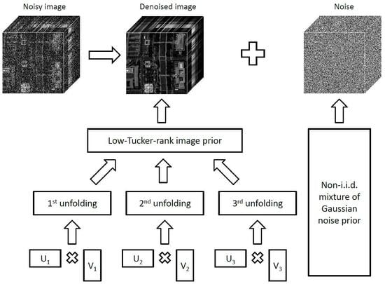
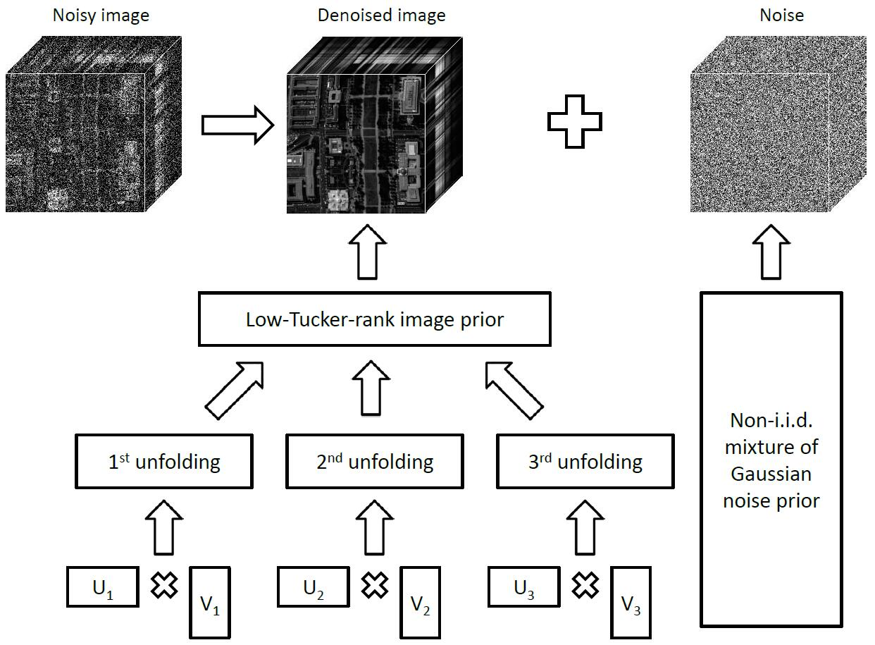
Noise removal is a fundamental problem in remote sensing image processing. Most existing methods, however, have not yet attained sufficient robustness in practice, due to more or less neglecting the intrinsic structures of remote sensing images and/or underestimating the complexity of realistic noise. In this paper, we propose a new remote sensing image denoising method by integrating intrinsic image characterization and robust noise modeling. Specifically, we use low-Tucker-rank tensor approximation to capture the global multi-factor correlation within the underlying image, and adopt a non-identical and non-independent distributed mixture of Gaussians (non-i.i.d. MoG) assumption to encode the statistical configurations of the embedded noise. Then, we incorporate the proposed image and noise priors into a full Bayesian generative model and design an efficient variational Bayesian algorithm to infer all involved variables by closed-form equations. Moreover, adaptive strategies for the selection of hyperparameters are further developed to make our algorithm free from burdensome hyperparameter-tuning. Extensive experiments on both simulated and real multispectral/hyperspectral images demonstrate the superiority of the proposed method over the compared state-of-the-art ones.

1. Introduction

Remote sensing images, such as multispectral images (MSIs) and hyperspectral images (HSIs), provide abundant spatial and spectral information of real scenes and play a central role in many real-world applications, such as urban planning, surveillance, and environmental monitoring. Unfortunately, during the acquisition process, remote sensing images are often corrupted by various kinds of noise, such as Gaussian noise, speckle noise, and stripe. Image denoising aims to recover an underlying clean image from its noisy observation, which is a fundamental problem in remote sensing image processing. To obtain effective signal-noise separations, denoising methods usually rely on some prior assumptions imposed on the image and noise components.

One of the key issues in denoising methods is the rational design of an image prior, which encourages some expected properties of the denoised image. As a significant property of remote sensing images, low-rankness means that high-dimensional image data lie in a low-dimensional subspace, which can also be considered to be sparsity over a learned basis. Methods based on low-rankness along this line can be categorized into two classes: matrix-based and tensor-based ones. Matrix-based methods perform low-rank matrix approximation on the unfolding (tensor matricization) of the noisy image along the spectral mode. To obtain an efficient low-rank solution, low-rank matrix factorization methods factorize the objective matrix into a product of two flat ones [1,2,3,4,5,6,7,8,9]; rank minimization methods penalize some surrogates of the rank function, such as the convex envelope nuclear norm [10,11,12] or tighter non-convex metrics, e.g., log-determinant penalty [13], Schatten p-norm [14,15], $\gamma$-norm (Laplace function) [16], and truncated/weighted nuclear norm [17,18]. These matrix-based methods, however, can capture only the spectral correlation but ignore the global multi-factor correlation in remote sensing images, which usually leads to suboptimal results under severe noise corruption. On the other hand, tensor-based methods explicitly model the underlying image as a low-rank tensor, by solving a tensor decomposition model or minimizing the corresponding induced tensor rank [19]. Representative works include CANDECOMP/PARAFAC (CP) decomposition with CP rank [20,21,22], Tucker decomposition with Tucker rank [23,24,25,26,27], tensor singular value decomposition (t-SVD) with tubal rank [28,29], and tensor train (TT) decomposition with TT rank [30,31,32]. Considering that each tensor decomposition represents a specific type of high-dimensional data structure, recent works attempt to combine the merits of different low-rank tensor models, such as the hybrid CP-Tucker model [33] and the Kronecker-basis-representation (KBR)-based tensor sparsity measure [34,35]. By characterizing the correlations across both spatial and spectral modes, the above tensor-based methods have the advantage of preserving the intrinsic multilinear structure of remote sensing images, achieving state-of-the-art denoising performance.

Another critical issue in current denoising methods is the choice of a noise prior, which characterizes the statistical properties of the data noise. This is generally realized by imposing certain assumptions on the noise distribution, leading to specific loss functions between the noisy image and the denoising result. Two traditional noise priors are the Gaussian prior [1,2,21,24] ($L_2$-norm loss) and the Laplacian prior [5,36,37] ($L_1$-norm loss), which are widely used for suppressing dense noise and sparse noise (outlier), respectively. A combination of Gaussian and Laplacian priors [12,27,29,38] ($L_1+L_2$ loss) is commonly considered in mixed noise removal. However, these priors are generally not flexible enough to fit the noise in real applications, whose distributions are much more complicated than Gaussian/Laplacian or a simple mixture of them. To handle such complex noise, several works model the noise with a mixture of Gaussians (MoG) distribution [3,4,8] (weighted-$L_2$ loss), due to its universal approximation capability to any continuous probability density function [39]. Later, MoG has been generalized to a mixture of exponential power (MoEP) distribution [6] (weighted-$L_p$ loss) for further flexibility and adaptivity. Despite the sophistication of the above priors, they all assume that the noise is independent and identically distributed (i.i.d.), which is still limited in handling realistic noise with non-i.i.d. statistical structures. In remote sensing images, the noise across different bands always exhibits evident distinctions in configuration and magnitude. To encode such noise characteristics, recent works impose non-i.i.d. assumptions on the noise distribution, such as non-i.i.d. MoG [7] and Dirichlet process Gaussian mixture [9,40], resulting in better noise fitting capability and higher denoising accuracy.

Some attempts have been presented to combine the advantages of recent developments in image characterization and noise modeling. To the best of our knowledge, only several studies are constructed as follows. Chen et al. [41] proposed a robust tensor factorization method based on CP decomposition and MoG noise assumption. However, their model does not consider uncertainty information of latent variables, such as the CP factor matrices and the MoG parameters, and thus is prone to overfitting due to point estimations of these variables by optimization-based approaches. To overcome this defect, Luo et al. [42] formulated the robust CP decomposition with MoG noise assumption as a full Bayesian model, in which all latent variables are given prior distributions and inferred under a variational Bayesian framework. Considering that CP decomposition cannot well capture the correlations along different tensor modes, Chen et al. [43] further integrated Tucker decomposition and MoG noise modeling into a generalized robust tensor factorization framework. However, this method also suffers from the overfitting problem and requires some critical hyperparameters to be manually specified, such as the tensor rank and the number of MoG components. Moreover, all the above methods impose an i.i.d. assumption on the data noise, which still under-estimates the complexity of realistic noise and thus leaves room for further improvement.

To overcome the aforementioned issues, in this paper we propose a new remote sensing image denoising method by taking into consideration the intrinsic properties of both remote sensing images and realistic noise. The main contribution of this work is summarized below.

• We formulate the image denoising problem as a full Bayesian generative model, in which a low-Tucker-rank image prior is exploited to characterize the intrinsic low-rank tensor structure of the underlying image, and a non-i.i.d. MoG noise prior is adopted to encode the complex and distinct statistical structures of the embedded noise.
• We design a variational Bayesian algorithm for an efficient solution to the proposed model, where each variable can be updated in closed-form. Moreover, we develop adaptive strategies for the selection of involved hyperparameters, to make our algorithm free from burdensome hyperparameter-tuning.
• We conduct extensive denoising experiments on both simulated and real MSIs/HSIs, and the results show the superiority of the proposed method over the compared state-of-the-art ones.

The rest of the paper is organized as follows. Section 2 introduces some notation used throughout the paper. Section 3 describes the proposed model and the corresponding variational inference algorithm. Section 4 presents experimental results and discussions. Section 5 concludes the paper.

2. Notation

We use boldface Euler script letters for tensors, e.g., $𝓐$, boldface uppercase letters for matrices, e.g., A, boldface lowercase letters for vectors, e.g., a, and lowercase letters for scalars, e.g., a. In particular, we use I, 0, and 1 for identity matrices, arrays of all zeros, and arrays of all ones, respectively. We use a pair of lowercase and uppercase letters for an index and its upper bound, e.g., $i=1,\dots ,I$. We use Matlab expressions to denote elements and subarrays, e.g., $\mathbf{a}\left(i\right)$, $\mathbf{A}(i,:)$, and $𝓐(i,:,:)$.

Given a tensor $𝓐\in {\mathbb{R}}^{I_1\times \dots \times I_D}$ ($𝓐$ reduces to a matrix when $D=2$ or a vector when $D=1$). The Frobenius norm and the 1-norm of $𝓐$ are, respectively, defined as

$${\parallel 𝓐\parallel }_F:=\sqrt{{\sum }_{i_1,\dots ,i_D=1}^{I_1,\dots ,I_D}𝓐{(i_1,\dots ,i_D)}^2}{\mathrm{and}\parallel 𝓐\parallel }_1:={\sum }_{i_1,\dots ,i_D=1}^{I_1,\dots ,I_D}|𝓐(i_1,\dots ,i_D)|.$$

For a given dimension $d\in \{1,\dots ,D\}$, the mode-d unfolding of $𝓐$ is denoted as ${\mathrm{unfold}}_d(𝓐)$ or, more compactly, as ${\mathbf{A}}_{\left(d\right)}$, whose size is $I_d\times (I_1\dots I_{d-1}{I}_{d+1}\dots I_D)$. The inverse process is denoted as ${\mathrm{fold}}_d\left({\mathbf{A}}_{\left(d\right)}\right):=𝓐$. More precisely, the tensor element $𝓐(i_1,\dots ,i_D)$ maps to the matrix element ${\mathbf{A}}_{\left(d\right)}(i_1^{\prime },i_2^{\prime })$ satisfying

$$i_1^{\prime }=i_d\mathrm{and}{i}_2^{\prime }=1+{\sum }_{k=1,k\ne d}^D(i_k-1){\prod }_{m=1,m\ne d}^{k-1}{I}_m,$$

see [19] for more details. The mapping between $(i_1,\dots ,i_D)$ and $(i_1^{\prime },i_2^{\prime })$ is denoted as

$${𝓐}^{I_1\times \dots \times I_D}(i_1,\dots ,i_D)={\mathbf{A}}_{\left(d\right)}^{I_d\times (I_1\dots I_{d-1}{I}_{d+1}\dots I_D)}(i_1^{\prime },i_2^{\prime }).$$

The Tucker rank of $𝓐$ is defined as a vector consisting of the ranks of its unfoldings, i.e.,

$$\mathrm{rank}(𝓐):=(\mathrm{rank}\left({\mathbf{A}}_{\left(1\right)}\right),\mathrm{rank}\left({\mathbf{A}}_{\left(2\right)}\right),\dots ,\mathrm{rank}\left({\mathbf{A}}_{\left(D\right)}\right)).$$

Additional notation is defined where it occurs.

3. Tucker Rank Minimization with Non-i.i.d. MoG Noise Modeling

This section is divided into three parts. Section 3.1 formulates the denoising problem as a full Bayesian model named Tucker rank minimization with non-i.i.d. MoG noise modeling (NMoG-Tucker). Section 3.2 presents a variational inference algorithm for solving the proposed model. Section 3.3 discusses the selection of hyperparameters involved in our model.

3.1. Bayesian Model Formulation

Let $𝓨,𝓧\in {\mathbb{R}}^{I\times J\times K}$ denote the noisy image and the underlying clean image, respectively. To characterize the low-Tucker-rank prior of remote sensing images, we consider the following low-rank matrix factorization of the mode-d unfoldings of $𝓨$ ($d=1,2,3$):

$${\mathbf{Y}}_{\left(d\right)}={\mathbf{U}}_d{\mathbf{V}}_d^T+{\mathbf{N}}_d,$$

(1)

where ${\mathbf{U}}_d\in {\mathbb{R}}^{I_d\times R_d}$ (${\left\{I_d\right\}}_{d=1}^3=\{I,J,K\}$) and ${\mathbf{V}}_d\in {\mathbb{R}}^{J_d\times R_d}$ (${\left\{J_d\right\}}_{d=1}^3=\{JK,IK,IJ\}$) are factor matrices with column number $R_d\le min(I_d,J_d)$, and ${\mathbf{N}}_d$ denotes the noise embedded in ${\mathbf{Y}}_{\left(d\right)}$. Below we formulate (1) as a full Bayesian model by imposing prior distributions on the involved variables.

Prior of the noise ${\mathbf{N}}_d$. We impose a non-i.i.d. MoG prior on ${\mathbf{N}}_d$ to characterize the complex structure of realistic noise. For simplicity of presentation, let us consider the tensor (We remark that ${𝓝}_d:={\mathrm{fold}}_d\left({\mathbf{N}}_d\right)$ depends on the dimension d because our model (1) does not enforce the equality between the low-rank components of $𝓨$ along different modes, i.e., ${\left\{{\mathrm{fold}}_d\left({\mathbf{U}}_d{\mathbf{V}}_d^T\right)\right\}}_{d=1}^3$, considering that the low-rankness degrees along different modes are generally not the same) ${𝓝}_d:={\mathrm{fold}}_d\left({\mathbf{N}}_d\right)\in {\mathbb{R}}^{I\times J\times K}$. We assume that each element in the k-th band of ${𝓝}_d$ follows a MoG distribution

$${𝓝}_d(i,j,k)\sim {\sum }_{l=1}^{L_d}{\Pi }_d(k,l)𝒩\left({𝓝}_d(i,j,k)\right|0,{\mathit{\tau }}_d{\left(l\right)}^{-1}),$$

(2)

where $L_d$ is the number of Gaussian components, ${\Pi }_d(k,:)\in {\mathbb{R}}^{L_d}$ is the mixing proportion satisfying ${\Pi }_d(k,l)>0$ and ${\sum }_{l=1}^{L_d}{\Pi }_d(k,l)=1$, and ${\mathit{\tau }}_d\in {\mathbb{R}}^{L_d}$ contains precisions of the Gaussian components. By introducing an indicator variable ${𝓩}_d\in {\{0,1\}}^{I\times J\times K\times L_d}$, we rewrite (2) as the following two-level generative process [44]:

$$\begin{array}{cc}\hfill & {𝓝}_d(i,j,k)\sim {\prod }_{l=1}^{L_d}𝒩{\left({𝓝}_d(i,j,k)\right|0,{\mathit{\tau }}_d{\left(l\right)}^{-1})}^{{𝓩}_d(i,j,k,l)},\hfill \\ \hfill & {𝓩}_d(i,j,k,:)\sim \mathrm{Multinomial}\left({𝓩}_d(i,j,k,:)\right|{\Pi }_d(k,:)),\hfill \end{array}$$

(3)

where ${𝓩}_d(i,j,k,:)\in {\{0,1\}}^{L_d}$ with ${\sum }_{l=1}^{L_d}{𝓩}_d(i,j,k,l)=1$ follows a multinomial distribution parameterized by ${\Pi }_d(k,:)$. Then, we impose conjugate priors on ${\mathit{\tau }}_d$ and ${\Pi }_d$ to obtain a complete Bayesian model,

$$\begin{array}{cc}\hfill & {\mathit{\tau }}_d\left(l\right)\sim \mathrm{Gamma}\left({\mathit{\tau }}_d\left(l\right)\right|a_0,b_0),\hfill \end{array}$$

(4)

$$\begin{array}{cc}\hfill & {\Pi }_d(k,:)\sim \mathrm{Dirichlet}\left({\Pi }_d(k,:)\right|{\alpha }_0\mathbf{1}),\hfill \end{array}$$

(5)

where $\mathrm{Gamma}(·|a_0,b_0)$ denotes the Gamma distribution with parameters $a_0$ and $b_0$, and $\mathrm{Dirichlet}(·|{\alpha }_0\mathbf{1})$ denotes the Dirichlet distribution parameterized by ${\alpha }_0\mathbf{1}\in {\mathbb{R}}^{L_d}$.

The proposed prior can characterize the following intrinsic properties of realistic noise.

• First, noise in each band exhibits complex statistical properties, which cannot be well captured by simple distributions such as Gaussian or Laplacian. We model the noise in each band by an i.i.d. MoG distribution, which is a universal approximator to any continuous distribution.
• Second, noise across different bands is non-identical in terms of structure and extent, due to sensor malfunctions and atmospheric conditions. This band-noise-distinctness nature is encoded by the band-dependent mixing proportion in MoG, leading to a non-i.i.d. noise distribution.
• Third, there is a strong correlation among the noise distributions in all bands, since real-life noise corruption is generally attributed to only a few main factors. In the proposed prior, the noise correlation is reflected by the fact that the MoG distributions of different bands share the same set of Gaussian components.

Prior of the factor matrices ${\mathbf{U}}_d$ and ${\mathbf{V}}_d$. Inspired by the sparse Bayesian learning principle [45], we assume that the columns of ${\mathbf{U}}_d$ and ${\mathbf{V}}_d$ are generated from the following Gaussian distributions:

$$\begin{array}{cc}\hfill & {\mathbf{U}}_d(:,r)\sim 𝒩\left({\mathbf{U}}_d(:,r)\right|0,{\mathit{\gamma }}_d{\left(r\right)}^{-1}\mathbf{I}),\hfill \end{array}$$

(6)

$$\begin{array}{cc}\hfill & {\mathbf{V}}_d(:,r)\sim 𝒩\left({\mathbf{V}}_d(:,r)\right|0,{\mathit{\gamma }}_d{\left(r\right)}^{-1}\mathbf{I}),\hfill \end{array}$$

(7)

where ${\mathit{\gamma }}_d\in {\mathbb{R}}^{R_d}$ denotes precisions following the conjugate prior

$${\mathit{\gamma }}_d\left(r\right)\sim \mathrm{Gamma}\left({\mathit{\gamma }}_d\left(r\right)\right|c_0,d_0).$$

(8)

Prior of the solution $𝓧$. Given the learned low-rank components along three modes, we assume that each element in $𝓧$ is generated from the following weighted multiplication of Gaussian distributions:

$$p(𝓧(i,j,k))=c{\prod }_{d=1}^3𝒩{(𝓧(i,j,k)|{\mathbf{U}}_d(i_d,:){\mathbf{V}}_d{(j_d,:)}^T,{\xi }^{-1})}^{\mathbf{w}\left(d\right)},$$

(9)

where $(i_d,j_d)$ maps to $(i,j,k)$ such that ${\mathbf{A}}_{\left(d\right)}^{I_d\times J_d}(i_d,j_d)={𝓐}^{I\times J\times K}(i,j,k)$, $\xi$ denotes the precision of the Gaussian distributions, $\mathbf{w}\in {\mathbb{R}}^3$ contains weights of the three modes satisfying $\mathbf{w}\left(d\right)>0$ and ${\sum }_{d=1}^3\mathbf{w}\left(d\right)=1$, and c is a normalization constant.

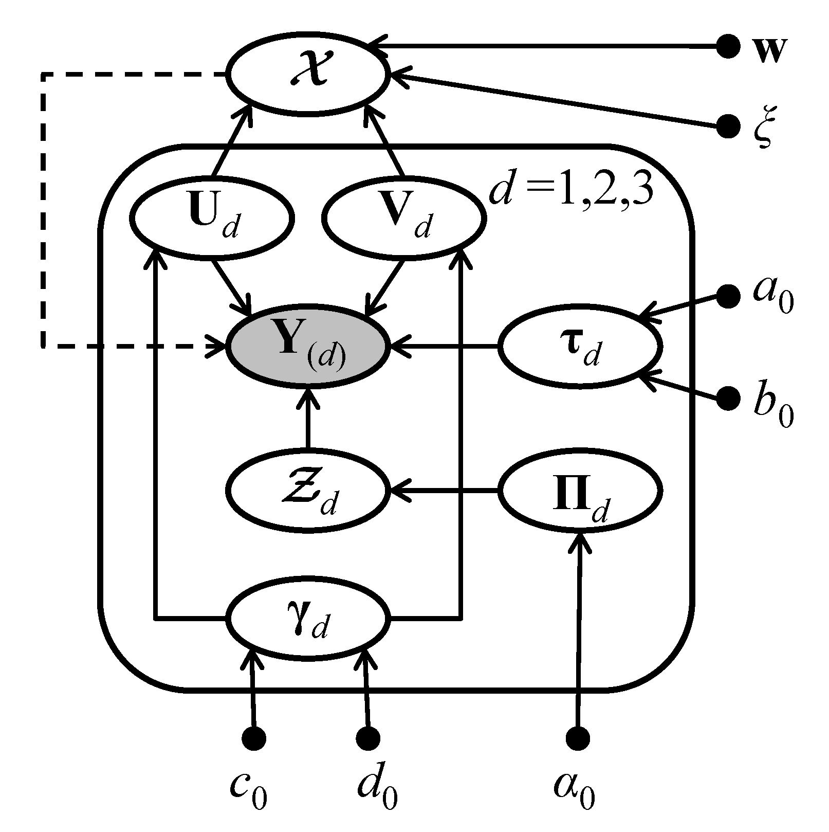
Full Bayesian model and posterior. We can construct a full Bayesian model by combining (1)–(9); the corresponding graphical model is shown in Figure 1. Then, the goal is to infer the posterior of all involved variables, which can be expressed as

$$\begin{array}{cc}\hfill & p(𝓧,{\{{\mathbf{U}}_d,{\mathbf{V}}_d,{\mathit{\gamma }}_d,{\mathit{\tau }}_d,{𝓩}_d,{\Pi }_d\}}_{d=1}^3|𝓨)\hfill \\ \hfill \propto & p(𝓧,{\{{\mathbf{U}}_d,{\mathbf{V}}_d,{\mathit{\gamma }}_d,{\mathit{\tau }}_d,{𝓩}_d,{\Pi }_d\}}_{d=1}^3,𝓨)\hfill \\ \hfill =& p(𝓧|{\{{\mathbf{U}}_d,{\mathbf{V}}_d\}}_{d=1}^3){\prod }_{d=1}^3\left\{p\left({\mathbf{Y}}_{\left(d\right)}\right|{\mathbf{U}}_d,{\mathbf{V}}_d,{\mathit{\tau }}_d,{𝓩}_d)p\left({\mathbf{U}}_d\right|{\mathit{\gamma }}_d)p\left({\mathbf{V}}_d\right|{\mathit{\gamma }}_d)p\left({\mathit{\gamma }}_d\right)p\left({\mathit{\tau }}_d\right)p\left({𝓩}_d\right|{\Pi }_d)p\left({\Pi }_d\right)\right\}.\hfill \end{array}$$

(10)

Optimization-based interpretation. From an optimization perspective, maximizing the posterior (10) is equivalent to minimizing its negative logarithm, i.e.,

$$\begin{array}{cc}\hfill & -lnp(𝓧,{\{{\mathbf{U}}_d,{\mathbf{V}}_d,{\mathit{\gamma }}_d,{\mathit{\tau }}_d,{𝓩}_d,{\Pi }_d\}}_{d=1}^3|𝓨)\hfill \end{array}$$

$$\begin{array}{ll}\hfill =-{\sum }_{d=1}^3& \left\{\mathbf{w}\left(d\right){\sum }_{i,j,k}ln𝒩(𝓧(i,j,k)|{\mathbf{U}}_d(i_d,:){\mathbf{V}}_d{(j_d,:)}^T,{\xi }^{-1})\right.\hfill \\ \hfill & +{\sum }_{i,j,k,l}{𝓩}_d(i,j,k,l)ln𝒩(𝓨(i,j,k)|{\mathbf{U}}_d(i_d,:){\mathbf{V}}_d{(j_d,:)}^T,{\mathit{\tau }}_d{\left(l\right)}^{-1})\hfill \\ \hfill & +{\sum }_{r}ln𝒩\left({\mathbf{U}}_d(:,r)\right|0,{\mathit{\gamma }}_d{\left(r\right)}^{-1}\mathbf{I})+{\sum }_{r}ln𝒩\left({\mathbf{V}}_d(:,r)\right|0,{\mathit{\gamma }}_d{\left(r\right)}^{-1}\mathbf{I})\hfill \\ \hfill & +{\sum }_{r}ln\mathrm{Gamma}\left({\mathit{\gamma }}_d\left(r\right)\right|c_0,d_0)+{\sum }_{l}ln\mathrm{Gamma}\left({\mathit{\tau }}_d\left(l\right)\right|a_0,b_0)\hfill \\ \hfill & \left.+{\sum }_{i,j,k}ln\mathrm{Multinomial}\left({𝓩}_d(i,j,k,:)\right|{\Pi }_d(k,:))+{\sum }_{k}ln\mathrm{Dirichlet}\left({\Pi }_d(k,:)\right|{\alpha }_{0}1)\right\}\hfill \end{array}$$

(11)

$$\begin{array}{cc}=\hfill & {\sum }_{d=1}^3\left\{\frac{\mathbf{w}\left(d\right)\xi }{2}{\parallel {\mathbf{X}}_{\left(d\right)}-{\mathbf{U}}_d{\mathbf{V}}_d^T\parallel }_F^2\right.+\frac{1}{2}\parallel {\mathrm{unfold}}_d\left({𝓗}_d\right)\odot ({\mathbf{Y}}_{\left(d\right)}-{\mathbf{U}}_d{\mathbf{V}}_d^T){\parallel }_F^2+\frac{1}{2}{\parallel {\mathbf{U}}_d\mathrm{diag}\left({\mathit{\gamma }}_d\right)\parallel }_F^2\hfill \\ \hfill & +\frac{1}{2}{\parallel {\mathbf{V}}_d\mathrm{diag}\left({\mathit{\gamma }}_d\right)\parallel }_F^2+{\sum }_r\left(d_0{\mathit{\gamma }}_d\left(r\right)-\left(\frac{I_d+J_d}{2}+c_0-1\right)ln{\mathit{\gamma }}_d\left(r\right)\right)\hfill \\ \hfill & +{\sum }_l\left(b_0{\mathit{\tau }}_d\left(l\right)-\left(\frac{1}{2}{\sum }_{i,j,k}{𝓩}_d(i,j,k,l)+a_0-1\right)ln{\mathit{\tau }}_d\left(l\right)\right)\hfill \\ \hfill & \left.+{\sum }_{i,j,k,l}\left(\frac{1}{2}ln\left(2\pi \right)-ln{\Pi }_d(k,l)\right){𝓩}_d(i,j,k,l)+{\sum }_{k,l}(1-{\alpha }_0)ln{\Pi }_d(k,l)\right\},\hfill \end{array}$$

(12)

where ${𝓗}_d\in {\mathbb{R}}^{I\times J\times K}$ contains the noise level estimations with ${𝓗}_d(i,j,k)=\sqrt{{\sum }_{l=1}^{L_d}{𝓩}_d(i,j,k,l){\mathit{\tau }}_d\left(l\right)}$, ⊙ denotes the element-wise multiplication, $\mathrm{diag}\left({\gamma }_d\right)$ denotes the diagonal matrix with the elements of ${\gamma }_d$ on its main diagonal. Below we illustrate the origin and the effect of each term in (12).

• The first ${\ell }_2$-norm term is derived from the weighted multiplication of Gaussians prior on the solution $𝓧$ (9). It forms $𝓧$ by penalizing the Euclidean distances between the unfoldings ${\left\{{\mathbf{X}}_{\left(d\right)}\right\}}_{d=1}^3$ and the low-rank components ${\left\{{\mathbf{U}}_d{\mathbf{V}}_d^T\right\}}_{d=1}^3$.
• The second weighted-${\ell }_2$-norm term is derived from the non-i.i.d. MoG prior on the noise ${\mathbf{N}}_d$ (3). It serves as a spatially varying loss function that suppresses the noise according to the local noise level estimations embedded in the weight matrix ${\mathrm{unfold}}_d\left({𝓗}_d\right)$.
• The third and the fourth weighted-${\ell }_2$-norm terms are derived from the Gaussian priors on the factor matrices ${\mathbf{U}}_d$ and ${\mathbf{V}}_d$ (6,7). They promote the joint group sparsity of $\{{\mathbf{U}}_d,{\mathbf{V}}_d\}$ in the unit of column pair $\{{\mathbf{U}}_d(:,r),{\mathbf{V}}_d(:,r)\}$, which implies the sparsity of ${\mathbf{U}}_d{\mathbf{V}}_d^T$ under rank-one bases ${\left\{{\mathbf{U}}_d(:,r){\mathbf{V}}_d{(:,r)}^T\right\}}_{r=1}^{R_d}$, i.e., the low-rankness of ${\mathbf{U}}_d{\mathbf{V}}_d^T$.
• The remainder terms are derived from the priors on the variables $\{{\mathit{\gamma }}_d,{\mathit{\tau }}_d,{𝓩}_d,{\Pi }_d\}$ and provide them with suitable regularization.

3.2. Approximate Variational Inference

We use the variational Bayesian (VB) method [44] to obtain an approximate inference of the posterior (10), since the exact solution is computationally intractable. Below we briefly introduce the general framework of VB, and then present the inference results for our model.

General framework of VB. Denoting by $\mathit{\theta }$ unobserved variables and by $\mathbf{D}$ observed data, VB aims to seek a variational distribution $q\left(\mathit{\theta }\right)$ to approximate the true posterior $p\left(\mathit{\theta }\right|\mathbf{D})$, by minimizing the Kullback–Leibler (KL) divergence between q and p, i.e.,

$$\underset{q\in \mathcal{C}}{min}\mathrm{KL}(q\parallel p):=-\int q\left(\mathit{\theta }\right)ln\left\{\frac{p\left(\mathit{\theta }\right|\mathbf{D})}{q\left(\mathit{\theta }\right)}\right\}\mathrm{d}\mathit{\theta },$$

(13)

where $\mathcal{C}$ imposes certain restrictions on q to make the minimization tractable. In general, q is restricted to have the factorization $q\left(\mathit{\theta }\right)={\prod }_i{q}_i\left({\mathit{\theta }}_i\right)$, where $\left\{{\mathit{\theta }}_i\right\}$ are disjoint groups of the variables in $\mathit{\theta }$. Under this assumption, one can approach the solution to (13) in an iterative way, by alternatively minimizing $\mathrm{KL}(q\parallel p)$ with respect to each $q_i\left({\mathit{\theta }}_i\right)$ while keeping the others fixed. More precisely, $q_i$ can be calculated by the following closed-form solution:

$$q_i\left({\mathit{\theta }}_i\right)=\frac{exp\left({\langle lnp(\mathit{\theta },\mathbf{D})\rangle }_{\mathit{\theta }\setminus {\mathit{\theta }}_i}\right)}{\int exp\left({\langle lnp(\mathit{\theta },\mathbf{D})\rangle }_{\mathit{\theta }\setminus {\mathit{\theta }}_i}\right)\mathrm{d}{\mathit{\theta }}_i},$$

(14)

where ${\langle ·\rangle }_{\mathit{\theta }\setminus {\mathit{\theta }}_i}$ denotes the expectation with respect to q over all variables except ${\mathit{\theta }}_i$.

Factorized form of the approximate posteriorq. We assume that the approximation of the posterior (10) has the following factorization (the subscripts of q are omitted without confusion):

$$\begin{array}{cc}\hfill & q(𝓧,{\{{\mathbf{U}}_d,{\mathbf{V}}_d,{\mathit{\gamma }}_d,{\mathit{\tau }}_d,{𝓩}_d,{\Pi }_d\}}_{d=1}^3)\hfill \\ \hfill =& {\prod }_{i,j,k=1}^{I,J,K}q(𝓧(i,j,k)){\prod }_{d=1}^3\left\{{\prod }_{i=1}^{I_d}q\left({\mathbf{U}}_d(i,:)\right)\right.{\prod }_{j=1}^{J_d}q\left({\mathbf{V}}_d(j,:)\right){\prod }_{r=1}^{R_d}q\left({\mathit{\gamma }}_d\left(r\right)\right)\hfill \\ \hfill & \left.{\prod }_{l=1}^{L_d}q\left({\mathit{\tau }}_d\left(l\right)\right){\prod }_{i,j,k,l=1}^{I,J,K,L_d}q\left({𝓩}_d(i,j,k,l)\right){\prod }_{k=1}^{K}q\left({\Pi }_d(k,:)\right)\right\}.\hfill \end{array}$$

(15)

According to (14), we give the analytical inference of each component in (15) as below.

Estimation of the low-rank component. Variables involved in the low-rank component are the factor matrices ${\{{\mathbf{U}}_d\in {\mathbb{R}}^{I_d\times R_d}\}}_{d=1}^3$ and ${\{{\mathbf{V}}_d\in {\mathbb{R}}^{J_d\times R_d}\}}_{d=1}^3$ with column-wise precisions ${\{{\mathit{\gamma }}_d\in {\mathbb{R}}^{R_d}\}}_{d=1}^3$, and the solution $𝓧\in {\mathbb{R}}^{I\times J\times K}$. For each row of ${\mathbf{U}}_d$, we have that

$$q\left({\mathbf{U}}_d(i,:)\right)=𝒩\left({\mathbf{U}}_d(i,:)\right|{\mathsf{\mu }}_{{\mathbf{U}}_d(i,:)},{\mathit{\Sigma }}_{{\mathbf{U}}_d(i,:)}),$$

(16)

with covariance ${\mathit{\Sigma }}_{{\mathbf{U}}_d(i,:)}\in {\mathbb{R}}^{R_d\times R_d}$ and mean ${\mathsf{\mu }}_{{\mathbf{U}}_d(i,:)}\in {\mathbb{R}}^{R_d}$ given by

$$\begin{array}{cc}\hfill & {\mathit{\Sigma }}_{{\mathbf{U}}_d(i,:)}={\left({\sum }_{j=1}^{J_d}\left(\mathbf{w}\left(d\right)\xi +{\sum }_{l=1}^{L_d}\langle {𝓩}_d(i^{\prime },j^{\prime },k^{\prime },l)\rangle \langle \mathit{\tau }\left(l\right)\rangle \right)\langle {\mathbf{V}}_d{(j,:)}^T{\mathbf{V}}_d(j,:)\rangle +\mathrm{diag}\left(\langle {\mathit{\gamma }}_d\rangle \right)\right)}^{-1},\hfill \\ \hfill & {\mathsf{\mu }}_{{\mathbf{U}}_d(i,:)}={\sum }_{j=1}^{J_d}\left(\mathbf{w}\left(d\right)\xi \langle 𝓧(i^{\prime },j^{\prime },k^{\prime })\rangle +{\sum }_{l=1}^{L_d}\langle {𝓩}_d(i^{\prime },j^{\prime },k^{\prime },l)\rangle \langle \mathit{\tau }\left(l\right)\rangle 𝓨(i^{\prime },j^{\prime },k^{\prime })\right)\langle {\mathbf{V}}_d(j,:)\rangle {\mathit{\Sigma }}_{{\mathbf{U}}_d(i,:)},\hfill \end{array}$$

where $(i^{\prime },j^{\prime },k^{\prime })$ maps to $(i,j)$ such that ${𝓐}^{I\times J\times K}(i^{\prime },j^{\prime },k^{\prime })={\mathbf{A}}_{\left(d\right)}^{I_d\times J_d}(i,j)$. Similarly, for each row of ${\mathbf{V}}_d$, we have that

$$q\left({\mathbf{V}}_d(j,:)\right)=𝒩\left({\mathbf{V}}_d(j,:)\right|{\mu }_{{\mathbf{V}}_d(j,:)},{\mathit{\Sigma }}_{{\mathbf{V}}_d(j,:)}),$$

(17)

where

$$\begin{array}{cc}\hfill & {\mathit{\Sigma }}_{{\mathbf{V}}_d(j,:)}={\left({\sum }_{i=1}^{I_d}\left(\mathbf{w}\left(d\right)\xi +{\sum }_{l=1}^{L_d}\langle {𝓩}_d(i^{\prime },j^{\prime },k^{\prime },l)\rangle \langle \mathit{\tau }\left(l\right)\rangle \right)\langle {\mathbf{U}}_d{(i,:)}^T{\mathbf{U}}_d(i,:)\rangle +\mathrm{diag}\left(\langle {\mathit{\gamma }}_d\rangle \right)\right)}^{-1},\hfill \\ \hfill & {\mathsf{\mu }}_{{\mathbf{V}}_d(j,:)}={\sum }_{i=1}^{I_d}\left(\mathbf{w}\left(d\right)\xi \langle 𝓧(i^{\prime },j^{\prime },k^{\prime })\rangle +{\sum }_{l=1}^{L_d}\langle {𝓩}_d(i^{\prime },j^{\prime },k^{\prime },l)\rangle \langle \mathit{\tau }\left(l\right)\rangle 𝓨(i^{\prime },j^{\prime },k^{\prime })\right)\langle {\mathbf{U}}_d(i,:)\rangle {\mathit{\Sigma }}_{{\mathbf{V}}_d(j,:)}.\hfill \end{array}$$

For each element in ${\mathit{\gamma }}_d$, we have that

$$q\left({\mathit{\gamma }}_d\left(r\right)\right)=\mathrm{Gamma}\left({\mathit{\gamma }}_d\left(r\right)\right|c_{{\mathit{\gamma }}_d},d_{{\mathit{\gamma }}_d\left(r\right)}),$$

(18)

with parameters $c_{{\mathit{\gamma }}_d}\in \mathbb{R}$ and $d_{{\mathit{\gamma }}_d\left(r\right)}\in \mathbb{R}$ given by

$$\begin{array}{cc}\hfill & c_{{\mathit{\gamma }}_d}=c_0+\frac{1}{2}(I_d+J_d),\hfill \\ \hfill & d_{{\mathit{\gamma }}_d\left(r\right)}=d_0+\frac{1}{2}(\langle {\mathbf{U}}_d{(:,r)}^T{\mathbf{U}}_d(:,r)\rangle +\langle {\mathbf{V}}_d{(:,r)}^T{\mathbf{V}}_d(:,r)\rangle ).\hfill \end{array}$$

For each element in $𝓧$, we have that

$$q(𝓧(i,j,k))=𝒩(𝓧(i,j,k)|{\mu }_{𝓧(i,j,k)},{\xi }^{-1}),$$

(19)

with mean ${\mu }_{𝓧(i,j,k)}\in \mathbb{R}$ given by

$${\mu }_{𝓧(i,j,k)}={\sum }_{d=1}^3\mathbf{w}\left(d\right)\langle {\mathbf{U}}_d(i_d,:)\rangle \langle {\mathbf{V}}_d{(j_d,:)}^T\rangle ,$$

where $(i_d,j_d)$ maps to $(i,j,k)$ such that ${\mathbf{A}}_{\left(d\right)}^{I_d\times J_d}(i_d,j_d)={𝓐}^{I\times J\times K}(i,j,k)$.

Estimation of the noise component. Variables involved in the noise component are the precisions ${\{{\mathit{\tau }}_d\in {\mathbb{R}}^{L_d}\}}_{d=1}^3$, the mixing proportions ${\{{\Pi }_d\in {\mathbb{R}}^{K\times L_d}\}}_{d=1}^3$, and the indicator variables ${\{{𝓩}_d\in {\mathbb{R}}^{I\times J\times K\times L_d}\}}_{d=1}^3$. For each element in ${\mathit{\tau }}_d$, we have that

$$q\left({\mathit{\tau }}_d\left(l\right)\right)=\mathrm{Gamma}\left({\mathit{\tau }}_d\left(l\right)\right|a_{{\mathit{\tau }}_d\left(l\right)},b_{{\mathit{\tau }}_d\left(l\right)}),$$

(20)

with parameters $a_{{\mathit{\tau }}_d\left(l\right)}\in \mathbb{R}$ and $b_{{\mathit{\tau }}_d\left(l\right)}\in \mathbb{R}$ given by

$$\begin{array}{cc}\hfill a_{{\mathit{\tau }}_d\left(l\right)}=& a_0+\frac{1}{2}{\sum }_{i,j,k=1}^{I,J,K}\langle {𝓩}_d(i,j,k,l)\rangle ,\hfill \\ \hfill b_{{\mathit{\tau }}_d\left(l\right)}=& b_0+\frac{1}{2}{\sum }_{i,j,k=1}^{I,J,K}\langle {𝓩}_d(i,j,k,l)\rangle \langle {(𝓨(i,j,k)-{\mathbf{U}}_d(i_d,:){\mathbf{V}}_d{(j_d,:)}^T)}^2\rangle ,\hfill \end{array}$$

where $(i_d,j_d)$ maps to $(i,j,k)$ such that ${\mathbf{A}}_{\left(d\right)}^{I_d\times J_d}(i_d,j_d)={𝓐}^{I\times J\times K}(i,j,k)$. For each row of ${\Pi }_d$, we have that

$$q\left({\Pi }_d(k,:)\right)=\mathrm{Dirichlet}\left({\Pi }_d(k,:)\right|{\mathit{\alpha }}_{{\Pi }_d(k,:)}),$$

(21)

with a parameter ${\mathit{\alpha }}_{{\Pi }_d(k,:)}\in {\mathbb{R}}^{L_d}$ given by

$${\mathit{\alpha }}_{{\Pi }_d(k,:)}\left(l\right)={\alpha }_0+{\sum }_{i,j=1}^{I,J}\langle {𝓩}_d(i,j,k,l)\rangle .$$

For each mode-4 fiber of ${𝓩}_d$, we have that

$$q\left({𝓩}_d(i,j,k,:)\right)=\mathrm{Multinomial}\left({𝓩}_d(i,j,k,:)\right|{\mathit{\rho }}_{{𝓩}_d(i,j,k,:)}),$$

(22)

with a parameter ${\mathit{\rho }}_{{𝓩}_d(i,j,k,:)}\in {\mathbb{R}}^{L_d}$ given by

$$\begin{array}{cc}\hfill {\mathit{\rho }}_{{𝓩}_d(i,j,k,:)}\left(l\right)=& cexp\left(-\frac{1}{2}ln\left(2\pi \right)+\frac{1}{2}\langle ln{\mathit{\tau }}_d\left(l\right)\rangle -\frac{1}{2}\langle ln{\mathit{\tau }}_d\left(l\right)\rangle \langle {(𝓨(i,j,k)-{\mathbf{U}}_d(i_d,:){\mathbf{V}}_d{(j_d,:)}^T)}^2\rangle \right.\hfill \\ \hfill & \left.+\langle ln{\Pi }_d(k,l)\rangle \right),\hfill \end{array}$$

where $(i_d,j_d)$ maps to $(i,j,k)$ such that ${\mathbf{A}}_{\left(d\right)}^{I_d\times J_d}(i_d,j_d)={𝓐}^{I\times J\times K}(i,j,k)$ and c is a normalization constant to ensure that ${\sum }_{l=1}^{L_d}{\mathit{\rho }}_{{𝓩}_d(i,j,k,:)}\left(l\right)=1$.

Pseudo-code and complexity analysis. The pseudo-code of the overall algorithm is summarized in Algorithm 1. The total complexity per iteration is approximately

$$\mathcal{O}\left({\sum }_{d=1}^3(I_d+J_d)R_d^3+I_d{J}_d{R}_d^2{L}_d\right),$$

(23)

where the first term is due to calculating the covariance matrices of ${\{{\mathbf{U}}_d,{\mathbf{V}}_d\}}_{d=1}^3$ (16,17), and the second term is due to calculating the parameters of ${\left\{{\mathbf{Z}}_d\right\}}_{d=1}^3$ (22). Since, in general, it holds $R_d\ll min(I_d,J_d)$, the complexity of our algorithm depends linearly on the size of the input data.

Algorithm 1. Variational Bayesian algorithm for NMoG-Tucker.

Input: Observed image $𝓨$.

Initialization:

1. Set the iteration index $t:=0$.

2. Initialize the low-rank component ${\{{\mathbf{U}}_d^{\left(t\right)},{\mathbf{V}}_d^{\left(t\right)},{\mathit{\gamma }}_d^{\left(t\right)}\}}_{d=1}^3$.

3. Initialize the noise component ${\{{\mathit{\tau }}_d^{\left(t\right)},{𝓩}_d^{\left(t\right)}\}}_{d=1}^3$.

Iteration: while not converged do

4. Given ${\{{\mathit{\tau }}_d^{\left(t\right)},{𝓩}_d^{\left(t\right)}\}}_{d=1}^3$, update the low-rank component ${\{{\mathbf{U}}_d^{(t+1)},{\mathbf{V}}_d^{(t+1)},{\mathit{\gamma }}_d^{(t+1)}\}}_{d=1}^3$ and ${𝓧}^{(t+1)}$ by (16)–(19).

5. Given ${\{{\mathbf{U}}_d^{(t+1)},{\mathbf{V}}_d^{(t+1)},{\mathit{\gamma }}_d^{(t+1)}\}}_{d=1}^3$, update the noise component ${\{{\mathit{\tau }}_d^{(t+1)},{\Pi }_d^{(t+1)},{𝓩}_d^{(t+1)}\}}_{d=1}^3$ by (20)–(22).

6. Set $t:=t+1$.

End while and output $𝓧={𝓧}^{\left(t\right)}$.

3.3. Selection of Hyperparameters

This section is devoted to the selection of hyperparameters involved in our model. We develop adaptive strategies to learn their values using the results of the current iteration, which makes our algorithm free from burdensome hyperparameter-tuning.

Selection of ${\left\{R_d\right\}}_{d=1}^3$. The hyperparameter ${\left\{R_d\right\}}_{d=1}^3$ controls the column numbers of the factor matrices ${\{{\mathbf{U}}_d,{\mathbf{V}}_d\}}_{d=1}^3$, which is an estimation of the Tucker rank of the solution. Since the true rank is often unknown in practice, we design an adaptive rank estimation strategy to improve the applicability of our method. The main idea consists of initializing $R_d$ with a large value and then decreasing it gradually by dropping singular values smaller than an adaptive threshold. More precisely, denoting by t the iteration index, we choose $R_d^{\left(t\right)}$ as

$$R_d^{\left(t\right)}:=max\left\{r|{\sigma }_d^{\left(t\right)}\left(r\right)\ge s_d^{\left(t\right)}\right\},$$

(24)

where ${\sigma }_d^{\left(t\right)}\subset [0,1]$ is a vector composed of the singular values of ${\mathbf{U}}_d^{\left(t\right)}{\left({\mathbf{V}}_d^{\left(t\right)}\right)}^T/{\parallel {\mathbf{U}}_d^{\left(t\right)}{\left({\mathbf{V}}_d^{\left(t\right)}\right)}^T\parallel }_2$ in a decreasing order (${\parallel ·\parallel }_2$ denotes the spectral norm, i.e., the largest singular value), $s_d^{\left(t\right)}\in [0,1]$ is a threshold given by

$$\begin{array}{cc}\hfill s_d^{\left(t\right)}:=& max\left(min\left({\sigma }_d^{\left(t\right)}\left(min\left\{i|{\sum }_{r>i}{\sigma }_d^{\left(t\right)}\left(r\right)<e^{\mathrm{upper}}{\parallel {\sigma }_d^{\left(t\right)}\parallel }_1\right\}\right),s_d^{(t-1)}\right),e^{\mathrm{lower}}{\sigma }_d^{\left(t\right)}\left(\mathrm{end}\right)\right),\hfill \end{array}$$

(25)

where $e^{\mathrm{upper}}\in (0,1)$ imposes an upper bound of the sum of the dropping singular values ${\left\{{\sigma }_d^{\left(t\right)}\left(r\right)\right\}}_{r>i}$, $e^{\mathrm{lower}}\in (0,1)$ imposes a lower bound of the threshold $s_d^{\left(t\right)}$, and ${\sigma }_d^{\left(t\right)}\left(\mathrm{end}\right)$ denotes the last element of ${\sigma }_d^{\left(t\right)}$. Our experiments use the default settings $e^{\mathrm{upper}}={10}^{-2}$ and $e^{\mathrm{lower}}=2/3$; the effects of these two hyperparameters on the denoising performance will be discussed in Section 4.4.

We make some comments on the proposed rank estimation strategy. First, the dropping singular values in each iteration carry at most 1% energy of ${\mathbf{U}}_d^{\left(t\right)}{\left({\mathbf{V}}_d^{\left(t\right)}\right)}^T$, leading to a robust rank decreasing process. Second, the threshold tends to decrease if a rank reduction occurs, i.e., $s_d^{\left(t\right)}>{\sigma }_d^{\left(t\right)}\left(\mathrm{end}\right)$, which avoids underestimating the true rank. Third, the threshold tends to increase if it is too small to trigger a rank reduction, i.e., $s_d^{\left(t\right)}<\frac{2}{3}{\sigma }_d^{\left(t\right)}\left(\mathrm{end}\right)$, which avoids overestimating the true rank.

Selection of $\mathbf{w}$. The hyperparameter $\mathbf{w}$ assigns relative weights of the three modes in the prior (9) and the posterior (19) of $𝓧$. We assume a positive correlation between $\mathbf{w}\left(d\right)$ and the low-rankness degree of ${\mathbf{X}}_{\left(d\right)}$, i.e., the more sparse the singular values of ${\mathbf{X}}_{\left(d\right)}$ are, the larger $\mathbf{w}\left(d\right)$ is. To measure the sparsity of singular values, we use the Gini index [46] (Here we take $G:=1-G^{\prime }$, where $G^{\prime }$ is the definition of the Gini index in [46]) defined by

$$G\left(\mathbf{a}\right):={\sum }_{i=1}^I\left(\frac{2i-1}{I}\right)\frac{\mathbf{a}\left(i\right)}{{\parallel \mathbf{a}\parallel }_1},$$

where $\mathbf{a}\in {\mathbb{R}}^I$ is a non-zero vector composed of nonnegative elements in a decreasing order. The Gini index takes positive values, and smaller values indicate better sparsity. Then, at the t-th iteration, we choose ${\mathbf{w}}^{\left(t\right)}\left(d\right)$ as

$${\mathbf{w}}^{\left(t\right)}\left(d\right):=cexp\left(-\frac{G\left({\sigma }_{{\mathbf{X}}_{\left(d\right)}}^{\left(t\right)}\right)}{{min}_{d}G\left({\sigma }_{{\mathbf{X}}_{\left(d\right)}}^{\left(t\right)}\right)}\right),$$

(26)

where ${\sigma }_{{\mathbf{X}}_{\left(d\right)}}^{\left(t\right)}$ contains the singular values of ${\mathbf{X}}_{\left(d\right)}$ in a decreasing order and c is a normalization constant to ensure that ${\sum }_{d=1}^3{\mathbf{w}}^{\left(t\right)}\left(d\right)=1$. Here we divide by ${min}_{d}G\left({\sigma }_{{\mathbf{X}}_{\left(d\right)}}^{\left(t\right)}\right)$ to measure the relative, rather than absolute, low-rankness degree.

Selection of $\xi$. The hyperparameter $\xi$ is the precision of the Gaussian distributions in the prior (9) and the posterior (19) of $𝓧$, which controls the contribution of $𝓧$ to the inference results of ${\left\{{\mathbf{U}}_d\right\}}_{d=1}^3$ (16) and ${\left\{{\mathbf{V}}_d\right\}}_{d=1}^3$ (17), or, equivalently, penalizes the distances between $𝓧$ and the low-rank components ${\left\{{\mathrm{fold}}_d\left({\mathbf{U}}_d{\mathbf{V}}_d^T\right)\right\}}_{d=1}^3$. For stability purpose, we initialize $\xi$ with a small value and increase it gradually until the convergence of $𝓧$. More precisely, at the t-th iteration, we set ${\xi }^{\left(t\right)}$ as

$${\xi }^{\left(t\right)}:={\xi }_0^{\left(t\right)}\frac{IJK}{\parallel 𝓨-{𝓧}^{\left(t\right)}{\parallel }_F^2},$$

(27)

where ${\xi }_0$ is an auxiliary hyperparameter updated as

$${\xi }_0^{\left(t\right)}:=\left\{\begin{array}{cc}1.5{\xi }_0^{(t-1)},\hfill & \mathrm{if}\frac{\parallel {𝓧}^{\left(t\right)}-{𝓧}^{(t-1)}{\parallel }_F^2}{\parallel {𝓧}^{(t-1)}{\parallel }_F^2}<\frac{\parallel {𝓧}^{(t-1)}-{𝓧}^{(t-2)}{\parallel }_F^2}{\parallel {𝓧}^{(t-2)}{\parallel }_F^2},\hfill \\ {\xi }_0^{(t-1)},\hfill & \mathrm{otherwise}.\hfill \end{array}\right.$$

Selection of ${\left\{L_d\right\}}_{d=1}^3$. The hyperparameter $L_d$ is the number of Gaussian components in the MoG prior of the noise ${\mathbf{N}}_d$ (2). To adaptively fit the noise distribution, we initialize $L_d$ with a relatively large value and iteratively decrease $L_d$ to $L_d-1$ if there exist two analogous Gaussian components satisfying

$$\frac{|{\mathit{\tau }}_d\left(l_1\right)-{\mathit{\tau }}_d\left(l_2\right)|}{|{\mathit{\tau }}_d\left(l_1\right)+{\mathit{\tau }}_d\left(l_2\right)|}\le 0.05.$$

For an initialization of $L_d$, our experiments use the default setting $(L_1^{\left(0\right)},L_2^{\left(0\right)},L_3^{\left(0\right)})=(8,8,8)$; its effects on the denoising performance will be discussed in Section 4.4.

Selection of other hyperparameters. The rest hyperparameters are $a_0$ and $b_0$ in the Gamma prior of ${\left\{{\mathit{\tau }}_d\right\}}_{d=1}^3$, $c_0$ and $d_0$ in the Gamma prior of ${\left\{{\mathit{\gamma }}_d\right\}}_{d=1}^3$, and ${\alpha }_0$ in the Dirichlet prior of ${\left\{{\Pi }_d\right\}}_{d=1}^3$. We simply fix them to ${10}^{-6}$ in a non-informative manner, to minimize their impacts on the inference process [44]. Our method performs stably well in all experiments under these simple settings.

4. Numerical Experiments

We evaluate the denoising performance of the proposed NMoG-Tucker method on synthetic data, MSIs, and HSIs.

Table 1. Summary of competing methods. Here ${\times }_d$ denotes the d-mode product [19], and ∘ denotes the vector outer product.

Competing Method	Data Prior	Noise Prior
LRMR [38]	Matrix rank constraint	Gaussian + sparse
	$\mathrm{rank}\left({\mathbf{X}}_{\left(3\right)}\right)\le r$
MoG-RPCA [4]	Low-rank matrix factorization	MoG
	${\mathbf{X}}_{\left(3\right)}=\mathbf{U}{\mathbf{V}}^T$
NMoG-LRMF [7]	Low-rank matrix factorization	Non-i.i.d. MoG
	${\mathbf{X}}_{\left(3\right)}=\mathbf{U}{\mathbf{V}}^T$
LRTA [24]	Tucker decomposition	Gaussian
	$𝓧=\mathit{C}{\times }_1{\mathbf{U}}_1{\times }_2{\mathbf{U}}_2{\times }_3{\mathbf{U}}_3$
PARAFAC [21]	CP decomposition	Gaussian
	$𝓧={\sum }_r{\lambda }_r{\mathbf{U}}_1(:,r)\circ {\mathbf{U}}_2(:,r)\circ {\mathbf{U}}_3(:,r)$
KBR-RPCA [35]	Kronecker-basis-representation	Gaussian + sparse
	$S(𝓧)={t\parallel \mathit{C}\parallel }_0+(1-t){\prod }_{d=1}^3\mathrm{rank}\left({\mathbf{X}}_{\left(d\right)}\right)$,
	where $𝓧=\mathit{C}{\times }_1{\mathbf{U}}_1{\times }_2{\mathbf{U}}_2{\times }_3{\mathbf{U}}_3$

lists six state-of-the-art competing methods on low-rank matrix/tensor approximation: matrix-based methods LRMR [38], MoG-RPCA [4], and NMoG-LRMF [7]; tensor-based methods LRTA [24], PARAFAC [21], and KBR-RPCA [35]. Parameters involved in all competing methods are set to default values or manually tuned for the best possible denoising performance. All experiments are conducted under Windows 10 and Matlab R2016a (Version 9.0.0.341360) running on a desktop with an Intel(R) Core(TM) i7-8700K CPU at 3.70 GHz and 32 GB memory.

We conduct both simulated and real denoising experiments. In simulated experiments, the noisy data are generated by adding synthetic noises to the original ones, and the denoising performance is evaluated by both quantitative measures and visual quality. In real experiments, the goal is to recover real-world data without knowing the ground-truths, and the denoising results are mainly judged by visual quality.

In simulated experiments, we use the following four quantitative measures: relative error (ReErr), erreur relative globale adimensionnelle de synthèse (ERGAS) [47], mean of peak signal-to-noise ratio (MPSNR), and mean of structural similarity (MSSIM) [48]. Denoting by ${𝓧}_{\mathrm{res}}\in {\mathbb{R}}^{I\times J\times K}$ an estimation to the original data ${𝓧}_{\mathrm{ori}}\in {\mathbb{R}}^{I\times J\times K}$, the four measures of ${𝓧}_{\mathrm{res}}$ with respect to ${𝓧}_{\mathrm{ori}}$ are defined as follows:

$$\begin{array}{cc}\hfill & \mathrm{ReErr}({𝓧}_{\mathrm{res}},{𝓧}_{\mathrm{ori}}):=\frac{\parallel {𝓧}_{\mathrm{res}}-{𝓧}_{\mathrm{ori}}{\parallel }_F}{\parallel {𝓧}_{\mathrm{ori}}{\parallel }_F},\hfill \\ \hfill & \mathrm{ERGAS}({𝓧}_{\mathrm{res}},{𝓧}_{\mathrm{ori}}):=100\sqrt{\frac{1}{K}{\sum }_{k=1}^K\frac{\parallel {𝓧}_{\mathrm{res}}(:,:,k)-{𝓧}_{\mathrm{ori}}{(:,:,k)\parallel }_F^2}{{\sum }_{i,j=1}^{I,J}{𝓧}_{\mathrm{ori}}(i,j,k)}},\hfill \\ \hfill & \mathrm{MPSNR}({𝓧}_{\mathrm{res}},{𝓧}_{\mathrm{ori}}):=\frac{1}{K}{\sum }_{k=1}^{K}10{log}_{10}\left(\frac{{255}^{2}IJ}{\parallel {𝓧}_{\mathrm{res}}(:,:,k)-{𝓧}_{\mathrm{ori}}{(:,:,k)\parallel }_F^2}\right),\hfill \\ \hfill & \mathrm{MSSIM}({𝓧}_{\mathrm{res}},{𝓧}_{\mathrm{ori}}):=\frac{1}{K}{\sum }_{k=1}^K\mathrm{SSIM}({𝓧}_{\mathrm{res}}(:,:,k),{𝓧}_{\mathrm{ori}}(:,:,k)),\hfill \end{array}$$

where the details of SSIM can be found in [48]. In general, better denoising results have smaller ReErr and ERGAS values and larger MPSNR and MSSIM values.

4.1. Synthetic Data Denoising

This section presents simulated experiments on synthetic data denoising. The original data are random low-rank tensors generated by the Tucker model with size $50\times 50\times 50$ and rank $(R_1,R_2,R_3)$, i.e., ${𝓧}_{\mathrm{ori}}:=\mathcal{C}{\times }_1{\mathbf{U}}_1{\times }_2{\mathbf{U}}_2{\times }_3{\mathbf{U}}_3$, where the core tensor $\mathcal{C}\in {\mathbb{R}}^{R_1\times R_2\times R_3}$ and each factor matrix ${\mathbf{U}}_d\in {\mathbb{R}}^{50\times R_d}$ ($d=1,2,3$) are drawn from standard Gaussian distribution. We consider two rank settings $(10,10,10)$ and $(20,15,10)$. The original data are normalized to have unit mean absolute value, i.e., $\parallel {𝓧}_{\mathrm{ori}}{\parallel }_1/{50}^3=1$. We test the following three kinds of synthetic noises.

• Gaussian noise: all entries mixed with Gaussian noise $𝒩(0,{0.1}^2)$.
• Gaussian + sparse noise: 80% entries mixed with Gaussian noise $𝒩(0,{0.1}^2)$ and 20% with additive uniform noise between $[-5,5]$.
• Mixture noise: 40% entries mixed with Gaussian noise $𝓝(0,{0.01}^2)$, 20% with Gaussian noise $𝒩(0,{0.2}^2)$, 20% with additive uniform noise between $[-5,5]$, and 20% missing (the locations of missing entries are not given as prior knowledge).

Table 2. Quantitative performance and execution time (in seconds) of different methods on synthetic data denoising. Every result is an average over ten trials with different realizations of both data and noise. The best results are highlighted in bold.

	Gaussian noise		Gaussian + sparse noise		Mixture noise
Rank (10,10,10)	ReErr	Time	ReErr	Time	ReErr	Time
Noisy data	7.41e-02	-	6.92e-01	-	8.08e-01	-
LRMR	4.09e-02	0.11	1.22e-01	2.27	4.40e-01	2.30
MoG-RPCA	3.35e-02	1.22	4.54e-02	6.22	3.21e-01	19.16
NMoG-LRMF	3.35e-02	4.78	4.15e-02	4.54	3.30e-01	15.29
LRTA	1.06e-02	0.12	1.43e-01	0.18	3.43e-01	0.42
PARAFAC	1.97e-02	5.19	2.67e-01	4.26	4.53e-01	4.04
KBR-RPCA	9.91e-03	2.93	1.44e-02	2.86	5.00e-02	2.91
NMoG-Tucker	1.00e-02	14.84	1.17e-02	31.14	3.25e-03	45.84
	Gaussian noise		Gaussian + sparse noise		Mixture noise
Rank (20,15,10)	ReErr	Time	ReErr	Time	ReErr	Time
Noisy data	7.56e-02	-	7.00e-01	-	8.12e-01	-
LRMR	4.27e-02	0.18	1.27e-01	2.09	4.58e-01	2.09
MoG-RPCA	3.42e-02	1.34	4.58e-02	5.01	2.84e-01	17.58
NMoG-LRMF	3.42e-02	3.72	4.22e-02	4.30	3.12e-01	15.17
LRTA	1.55e-02	0.14	2.04e-01	0.18	3.85e-01	0.36
PARAFAC	1.87e-01	5.10	3.17e-01	4.61	4.98e-01	4.18
KBR-RPCA	1.45e-02	2.45	2.16e-02	2.23	9.06e-02	3.12
NMoG-Tucker	1.47e-02	16.63	1.72e-02	34.62	1.97e-02	62.04

reports the ReErr values and execution time of different methods on synthetic data denoising, where every result is an average over ten trials with different realizations of both data and noise. Regarding the denoising accuracy, our method consistently attains comparable or lower ReErr values than the competing methods, and its superiority becomes more significant as the noise complexity increases. Regarding the computational speed, LRTA is generally the fastest method, while our method is the slowest in all cases. The relatively high cost of our algorithm is mainly due to two facts: computing variables corresponding to all three modes requires three times more calculations than those in matrix-based methods; updating the factor matrices row by row is much slower than updating them as a whole in other tensor-based methods. An acceleration of our implementation will be left to future research.

4.2. MSI Denoising

This section presents simulated experiments on MSI denoising. The original data are six MSIs (Beads, Cloth, Hairs, Jelly Beans, Oil Painting, Watercolors) from the Columbia MSI Database (http://www1.cs.columbia.edu/CAVE/databases/multispectral) [49] containing scenes of a variety of real-world objects. Each MSI is of size $512\times 512\times 31$ with intensity range scaled to $[0,1]$. We test the following two kinds of synthetic noises.

• Gaussian noise: all entries mixed with Gaussian noise $𝒩(0,{0.05}^2)$. The signal-to-noise-ratio (SNR) value averaged over all 31 bands and all six MSIs is $13.88$ dB.
• Mixture noise: 60% entries mixed with Gaussian noise $𝒩(0,{0.01}^2)$, 20% with Gaussian noise $𝓝(0,{0.2}^2)$, and 20% with additive uniform noise between $[-5,5]$. The SNR value averaged over all 31 bands and all six MSIs is $-14.38$ dB.

Table 3. Quantitative performance of different methods on MSI denoising. Every result is an average over six testing MSIs. The best results are highlighted in bold.

	Gaussian Noise			Mixture Noise
	MPSNR	MSSIM	ERGAS	MPSNR	MSSIM	ERGAS
Noisy image	26.02	0.8088	204.24	-2.24	0.0233	5287.19
LRMR	35.30	0.9631	72.70	20.38	0.6893	418.92
MoG-RPCA	31.31	0.8131	123.98	31.34	0.9475	125.40
NMoG-LRMF	32.88	0.9453	106.49	32.39	0.9531	146.44
LRTA	35.40	0.9575	71.53	20.61	0.4120	386.96
PARAFAC	26.82	0.7349	211.89	17.10	0.2496	569.36
KBR-RPCA	35.19	0.9637	73.95	33.43	0.9548	96.54
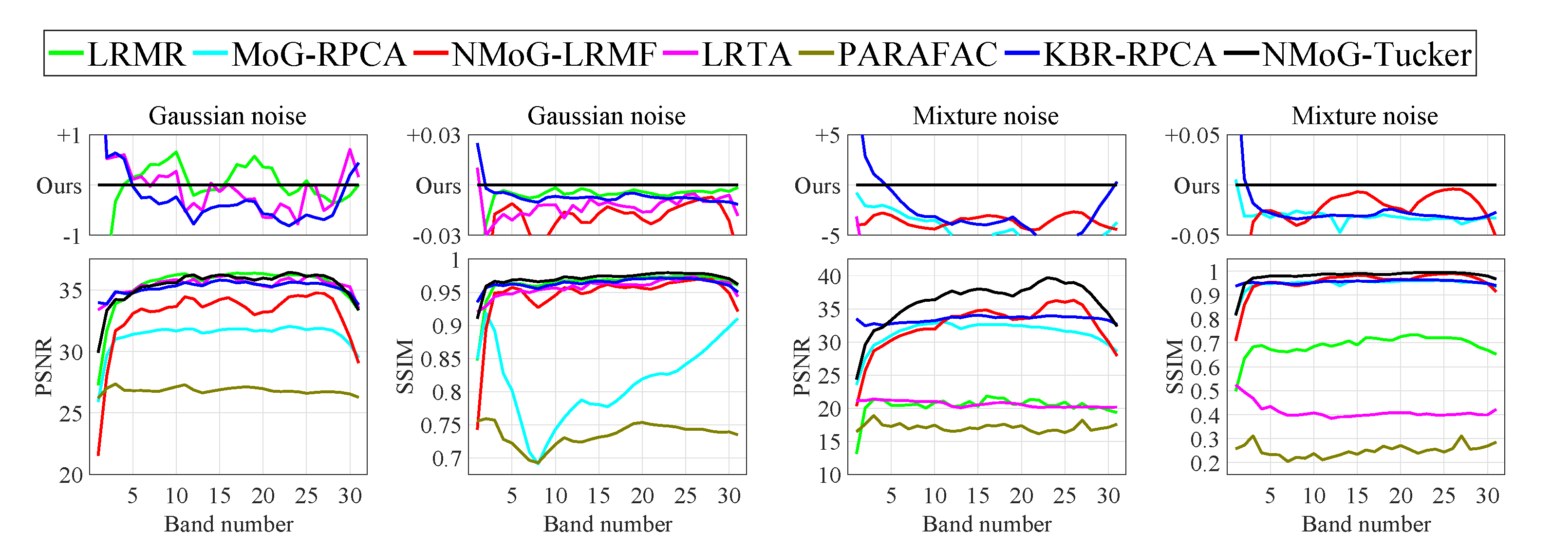
NMoG-Tucker	35.37	0.9703	71.49	36.02	0.9787	85.33

reports the quantitative performance of different methods on MSI denoising, where every result is an average over six testing MSIs. For Gaussian noise, our method achieves comparable denoising performance to LRMR, LRTA, and KBR-RPCA. For mixture noise, our method performs better than the competing methods in terms of all three quantitative measures, and KBR-RPCA is the second best.

Figure 2 shows the average PSNR and SSIM values across all bands of the denoising results by different methods. For easy observation of the details, we plot the differences between our results and the competing ones at larger scales. It can be observed that our method achieves comparable or better performance for most bands, while KBR-RPCA exhibits the best robustness over all bands.

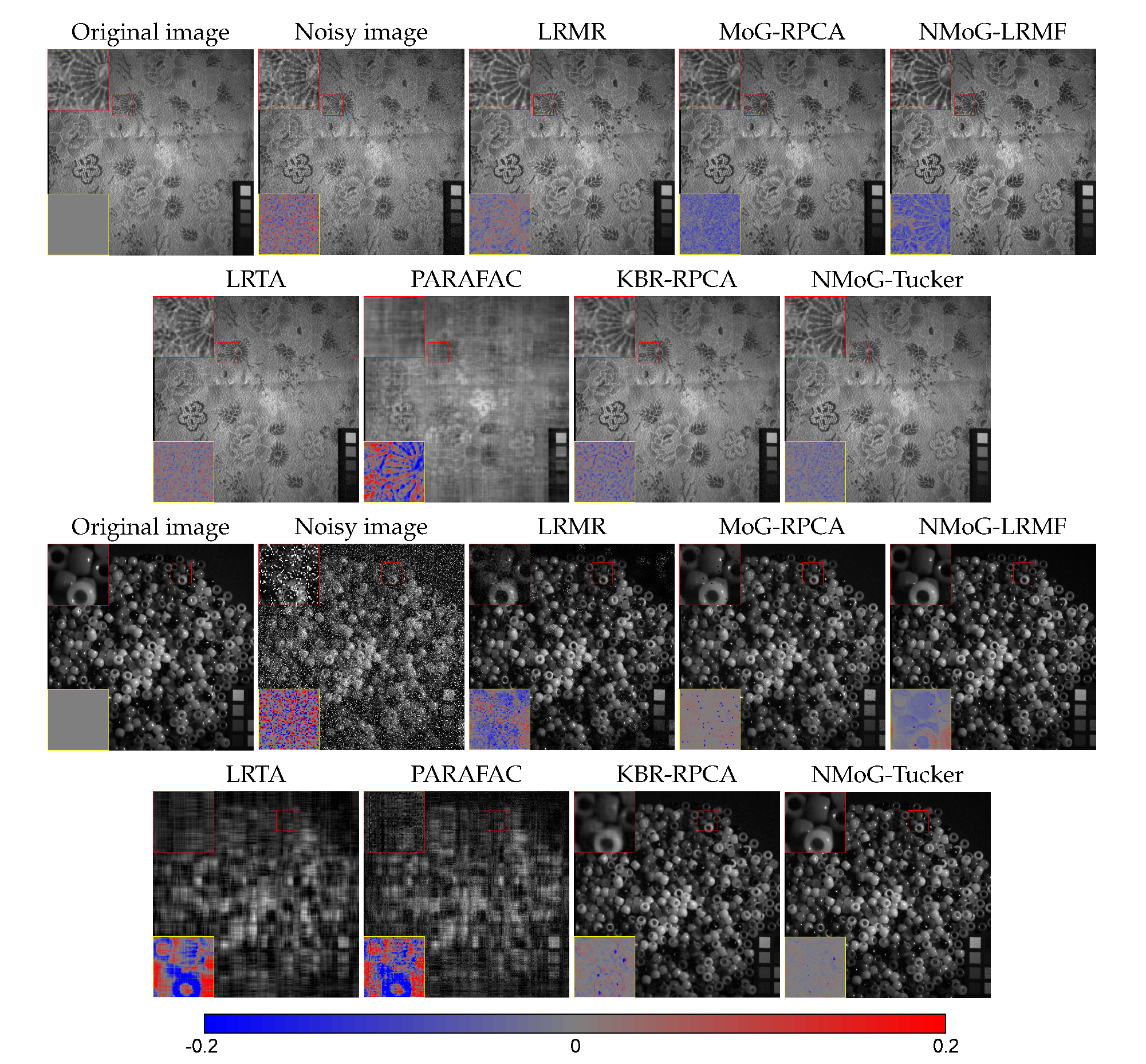
Figure 3 shows two examples on MSI denoising under Gaussian noise and mixture noise. These figures suggest that the results by the competing methods generally maintain some noise or alter image details, whereas our results exhibit higher visual quality in both noise removal and detail preservation. For better visualization, we enlarge a certain patch and show the corresponding error map, which highlights the difference between the denoised patch and the original one. A close inspection reveals that our error maps contain less color information than the competing ones, indicating that our method better recovers the spatial-spectral structures of the original MSIs.

4.3. HSI Denoising

We conduct both simulated and real experiments on HSI denoising.

Simulated HSI denoising. We adopt two original HSIs considered in NMoG-LRMF [7], i.e., a $200\times 200\times 160$ sub-image of Washington DC Mall (http://engineering.purdue.edu/~biehl/MultiSpec/hyperspectral.html ) (DCmall for short) and a $200\times 200\times 89$ sub-image of Cuprite (http://peterwonka.net/Publications/code/LRTC_Package_Ji.zip) [25]. The intensity range is scaled to $[0,1]$. To simulate the degradation scenarios in real-world HSIs, we test the following three kinds of synthetic noises.

• Gaussian noise: all entries mixed with Gaussian noise $𝒩(0,{0.05}^2)$. For DCmall, the SNR value of each band varies from 6 to 20 dB, and the mean SNR value of all 160 bands is 13.79 dB. For Cuprite, the SNR value of each band varies from 16 to 20 dB, and the mean SNR value of all 89 bands is 18.69 dB.
• Speckle noise: all bands are corrupted by non-i.i.d. speckle noise with signal-dependent intensity, which is simulated by multiplicative uniform noise with mean 1 and variance randomly sampled from $[0.001,0.5]$ for each band. For both DCmall and Cuprite, the SNR value of each band varies from 3 to 30 dB. The mean SNR value of all 160 bands in DCmall is 19.52 dB, and that of all 89 bands in Cuprite is 20.03 dB.
• Mixture noise: all bands are corrupted by non-i.i.d. Gaussian noise with zero-mean and band-dependent variances, and the SNR value of each band is uniformly sampled from 10 to 20 dB. Then, we randomly choose 90/50 bands in DCmall/Cuprite to add complex noises: the first 40/20 bands are corrupted by stripe noise with stripe number between $[20,40]$ and stripe intensity between $[-0.25,0.25]$; the middle 40/20 bands are corrupted by deadline with line number between $[5,15]$; $50\%$ to $70\%$ entries in the last 40/20 bands are corrupted by speckle noise with mean 1 and variance $0.3$. Thus, each band is randomly corrupted by one to three types of noises. For both DCmall and Cuprite, the SNR value of each band varies from 4 to 20 dB. The mean SNR value of all 160 bands in DCmall is 11.62 dB, and that of all 89 bands in Cuprite is 12.04 dB.

Table 4. Quantitative performance of different methods on simulated HSI denoising. Every result is an average over five trials with different noise realizations. The best results are highlighted in bold.

	Gaussian noise			Speckle noise			Mixture noise
DCmall	MPSNR	MSSIM	ERGAS	MPSNR	MSSIM	ERGAS	MPSNR	MSSIM	ERGAS
Noisy data	26.02	0.7627	187.93	31.65	0.8697	226.53	23.94	0.6988	316.59
LRMR	38.54	0.9848	43.35	38.44	0.9789	58.46	37.10	0.9785	58.66
MoG-RPCA	38.97	0.9865	41.59	33.85	0.9520	144.52	34.81	0.9597	110.30
NMoG-LRMF	39.47	0.9876	38.91	39.66	0.9847	59.58	38.68	0.9838	56.39
LRTA	36.86	0.9731	52.07	31.66	0.8698	226.17	24.05	0.7021	314.09
PARAFAC	32.02	0.9360	90.77	32.75	0.9410	89.04	28.81	0.8722	164.61
KBR-RPCA	37.31	0.9819	49.94	38.20	0.9844	48.77	36.82	0.9797	54.89
NMoG-Tucker	39.52	0.9877	38.68	40.23	0.9876	42.66	39.23	0.9865	44.51
	Gaussian noise			Speckle noise			Mixture noise
Cuprite	MPSNR	MSSIM	ERGAS	MPSNR	MSSIM	ERGAS	MPSNR	MSSIM	ERGAS
Noisy data	26.02	0.6953	124.07	27.23	0.7052	225.22	19.42	0.4071	327.75
LRMR	36.69	0.9668	38.03	35.59	0.9511	59.71	32.93	0.9300	60.28
MoG-RPCA	35.51	0.9697	43.46	31.62	0.9415	133.78	28.67	0.9101	119.08
NMoG-LRMF	36.67	0.9696	39.08	36.74	0.9737	59.43	33.77	0.9446	58.81
LRTA	34.69	0.9324	48.11	27.29	0.7070	222.79	21.01	0.4687	272.44
PARAFAC	29.41	0.8223	86.12	29.82	0.8395	85.87	25.81	0.7150	158.41
KBR-RPCA	35.49	0.9564	44.01	34.54	0.9611	51.75	32.70	0.9208	59.98
NMoG-Tucker	37.41	0.9706	35.59	38.72	0.9805	32.43	34.04	0.9462	51.58

presents the quantitative performance of different methods on simulated HSI denoising, where every result is an average over five trials with different noise realizations. Compared with the competing methods, our method consistently yields better performance in terms of MPSNR, MSSIM, and ERGAS in all cases.

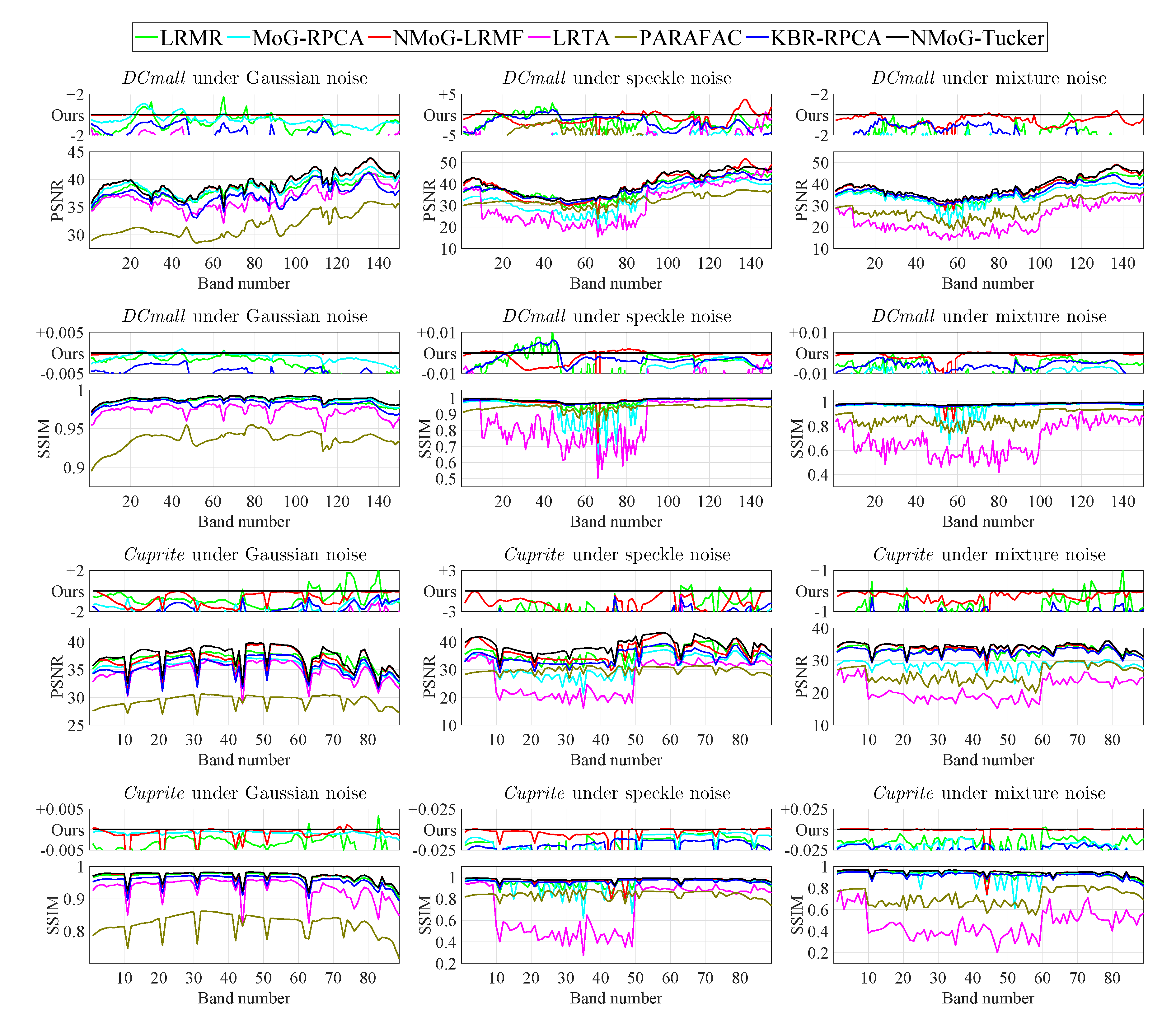
Figure 4 plots the average PSNR and SSIM values across all bands by different methods, as well as the differences between our results and the competing ones at larger scales. These results suggest that our method achieves leading quantitative performance for most bands. We also observe that the matrix-based competing methods LRMR, MoG-RPCA, and NMoG-LRMF suffer from sharp PSNR and SSIM drops at certain bands in the cases of speckle noise and mixture noise, e.g., bands 40–80 in DCmall and bands 40–60 in Cuprite. In comparison, our method does not exhibit such phenomenon, which demonstrates its robustness over entire HSI bands.

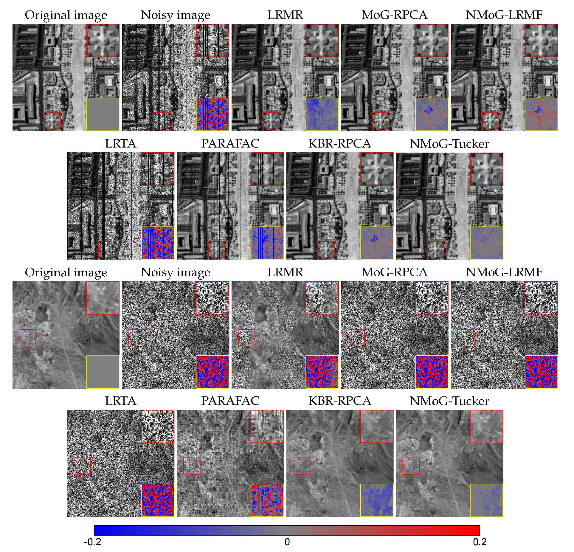
Figure 5 shows two denoising examples on typical bands in DCmall and Cuprite. The noisy band in DCmall is severely contaminated by a mixture of Gaussian noise, deadline, and speckle noise; the noisy band in in Cuprite is overwhelmed by heavy speckle noise. We observe that the matrix-based methods LRMR, MoG-RPCA, and NMoG-LRMF, although adopting flexible noise priors, cannot adequately separate the original HSIs from such severe degradations, especially for Cuprite with fewer spectral bands. As for tensor-based methods, LRTA can hardly reduce the noise, while PARAFAC leaves all the deadlines. Their poor performance is due to the Gaussian noise assumption, which is not able to fit complex noise. In comparison, adopting more intrinsic data and noise priors, KBR-RPCA and our method yield satisfactory denoising results in both cases. Compared with KBR-RPCA, our method preserves finer HSI structures with less residual noise, which can be seen from the demarcated patches and the corresponding error maps. Our better performance is mainly attributed to the non-i.i.d. MoG noise prior, which has a better fitting capability than the Gaussian + sparse assumption in the RPCA framework.

Real HSI denoising. Our experiment uses two real HSI datasets: Indian Pines (https://engineering.purdue.edu/~biehl/MultiSpec/hyperspectral.html ) of size $145\times 145\times 220$ and Urban (http://www.tec.army.mil/hypercube ) of size $307\times 307\times 210$. In both datasets, some bands are polluted by atmosphere and water absorption with little useful information. We do not remove them, to test the robustness of different methods under severe degradation. The intensity range of the input HSI is scaled to $[0,1]$.

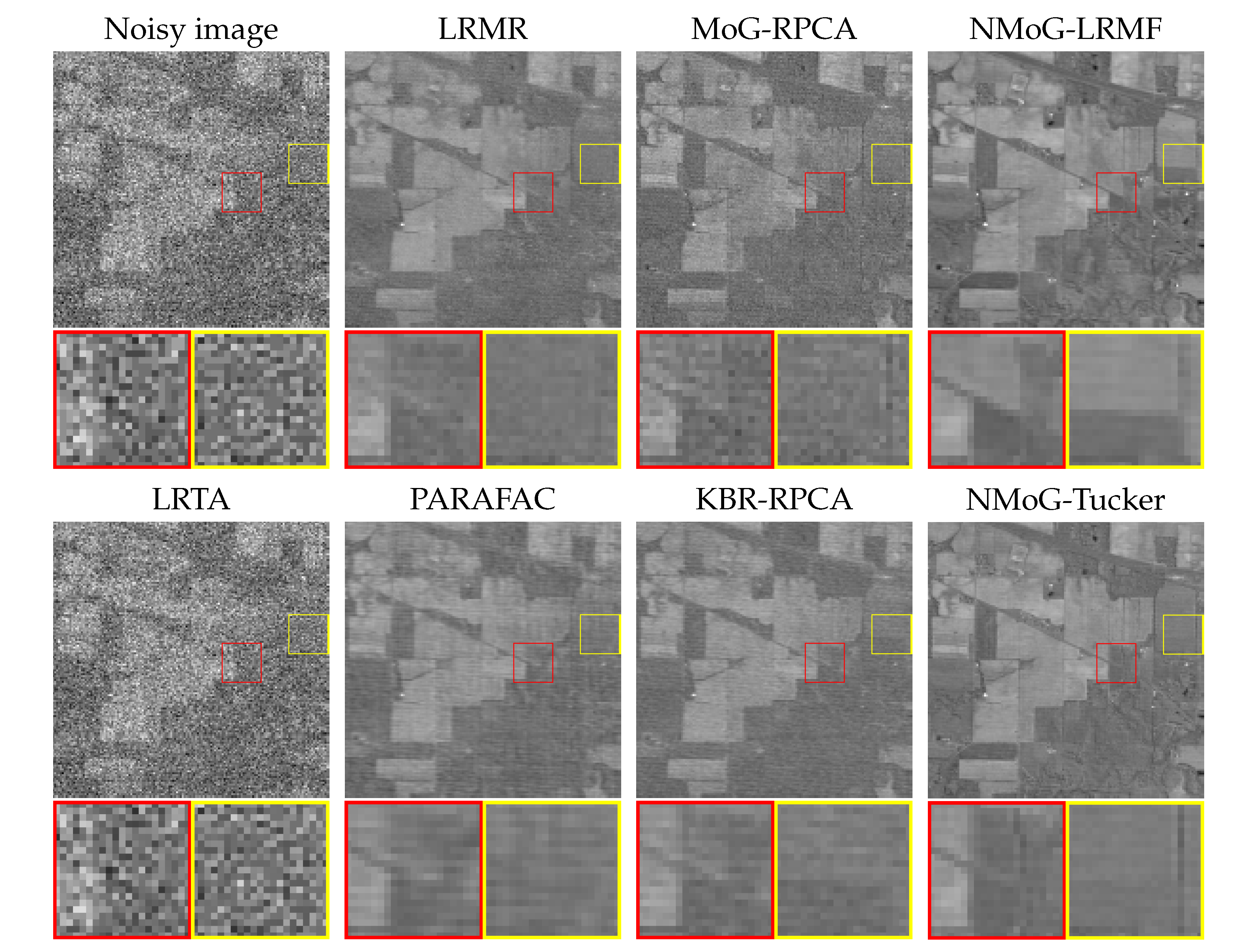
Figure 6 shows a denoising example on band 220 in Indian Pines. One can see that the original band is overwhelmed by noise with almost no useful information. From the denoising results by the competing methods, we observe that LRTA fails to handle such severe degradation; MoG-RPCA still leaves much noise in the whole image; LRMR, PARAFAC, and KBR remove more noise but simultaneously lose tiny image details; NMoG-LRMF yields a visually satisfactory result, but seems to produce false edges in the demarcated patches. On the other hand, the proposed method outperforms the competing methods in terms of both noise removal and detail preservation.

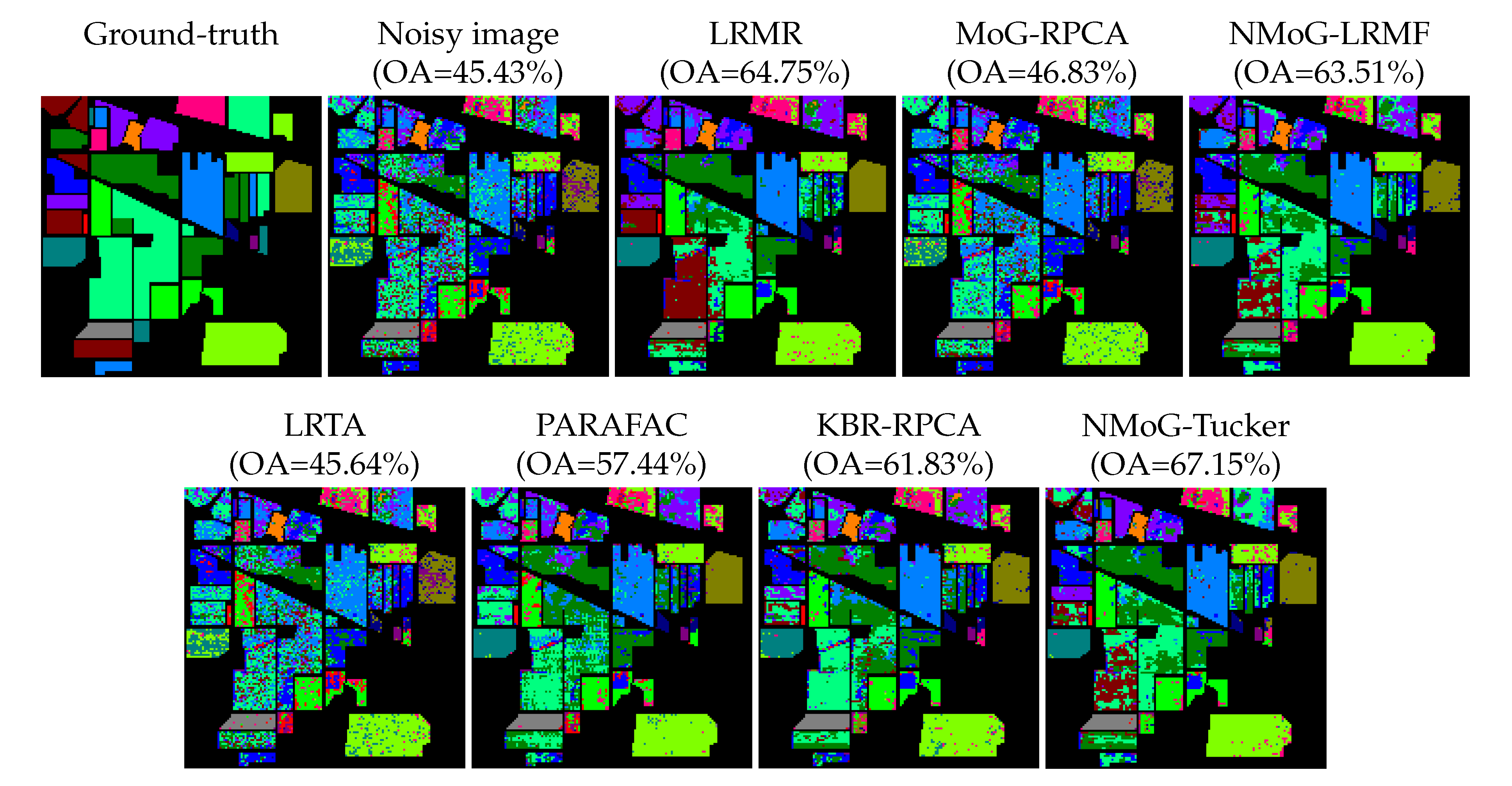
Figure 7 presents a classification example on Indian Pines. This test aims to provide a task-oriented evaluation of the denoising performance of different methods, from the perspective of the influence on the classification accuracy. In the ground-truth classification result, a total of 10249 samples are divided into 16 classes, and the number of samples in each class ranges from 20 to 2455. To conduct a supervised classification, we randomly choose ten samples for each class as training data, and use the remaining samples in each class as testing data. Then, the support vector machine (SVM) classification [50] is performed on the noisy image and its denoised versions by different methods, and the classification results are quantitatively evaluated by overall accuracy (OA). It can be seen that noise corruption significantly limits the classification accuracy, and the classification results of the denoised HSIs are more or less improved since the noise is suppressed. Among all denoising methods, our method leads to the highest OA value, demonstrating its superiority in benefiting the SVM classification.

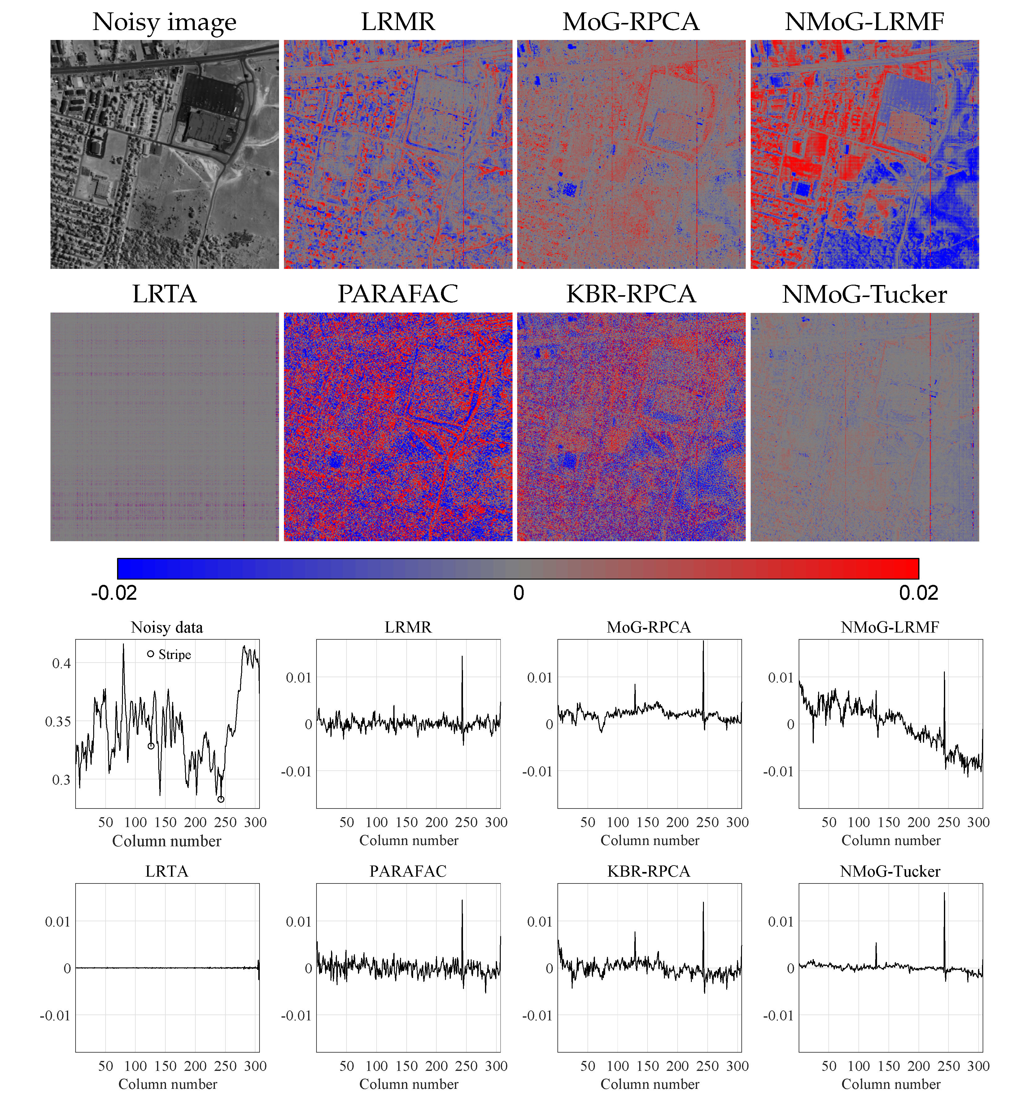
Figure 8 shows a denoising example on band 99 in Urban under slight noise. In this example, the original band is mainly corrupted by several vertical stripes with intensity 0.01∼0.02. To visually evaluate the denoising performance, we show color maps of the noise components estimated by different methods, which should highlight the underlying noise with as few image structures as possible. For better visualization, we also plot the corresponding vertical mean profiles. From these results, we observe that LRTA fails to recognize the stripes, while the other competing methods can detect the stripes but simultaneously remove structural information of the original image. In comparison, our method extracts clearly the stripes with very few image features, indicating a more accurate signal-noise separation.

Figure 9 displays a denoising example on band 206 in Urban under severe noise, including the noisy/denoised bands and the corresponding horizontal mean profiles. One can see that the original band is contaminated by a mixture of stripes, deadlines, and other complex noise, leading to rapid fluctuations in the horizontal mean profile. Regarding the denoising results by different methods, LRTA can hardly suppress the noise; LRMR, MoG-RPCA, PARAFAC, and KBR-RPCA still leave some horizontal stripes, and the corresponding curves show evident fluctuations; NMoG-LRMF removes the noise and produces a smooth curve, but it also introduces some spectral distortions in certain regions, such as the red demarcated patch. Comparatively, our method effectively attenuates the noise and simultaneously reveals the original spatial-spectral information, providing a better trade-off between noise removal and detail preservation.

4.4. Discussion

In Section 3.3, we have developed adaptive strategies for the selection of hyperparameters involved in our model. These strategies themselves also introduce additional hyperparameters, which are fixed as default settings in our experiments. This section discusses the selection of those hyperparameters and tests their effects on the denoising performance.

The selection of $e^{\mathrm{upper}}$ and $e^{\mathrm{lower}}$. The hyperparameters $e^{\mathrm{upper}}$ and $e^{\mathrm{lower}}$ are introduced in the update formula of the threshold $s_d^{\left(t\right)}$ (25), in order to determine the Tucker rank estimation ${\left\{R_d^{\left(t\right)}\right\}}_{d=1}^3$. In (25), $e^{\mathrm{upper}}$ controls the upper bound of the sum of the dropping singular values in each iteration. In general, a small $e^{\mathrm{upper}}$ leads to a slow but stable rank decreasing process; a large $e^{\mathrm{upper}}$ makes this process fast but aggressive, increasing the risk of underestimating the true rank. On the other hand, $e^{\mathrm{lower}}$ in (25) controls the lower bound of the threshold $s_d^{\left(t\right)}$, which provides a mechanism for avoiding overestimating the true rank. Roughly speaking, larger values of $e^{\mathrm{lower}}$ make our algorithm easier to reduce the rank. Please note that a too large $e^{\mathrm{lower}}$ tends to underestimate the true rank, e.g., if one sets $e^{\mathrm{lower}}=1$, then the rank decreasing process cannot stop until the rank reduces to zero.

Table 5. ReErr values and estimated ranks of our method under different settings of $e^{\mathrm{upper}}$ and $e^{\mathrm{lower}}$. This test is based on synthetic data denoising, and the original data are with size $50\times 50\times 50$ and Tucker rank $(20,15,10)$. The best results are highlighted in bold.

		Gaussian Noise		Gaussian + Sparse Noise		Mixture Noise
${\mathit{e}}^{\mathbf{upper}}$	${\mathit{e}}^{\mathbf{lower}}$	ReErr	${\left\{{\mathit{R}}_{\mathit{d}}^{\left(\mathbf{end}\right)}\right\}}_{\mathit{d}=1}^3$	ReErr	${\left\{{\mathit{R}}_{\mathit{d}}^{\left(\mathbf{end}\right)}\right\}}_{\mathit{d}=1}^3$	ReErr	${\left\{{\mathit{R}}_{\mathit{d}}^{\left(\mathbf{end}\right)}\right\}}_{\mathit{d}=1}^3$
	1/2	1.45e-02	$(20,15,10)$	1.69e-02	$(20,15,10)$	2.35e-2	$(20,15,10)$
${10}^{-3}$	2/3	1.45e-02	$(20,15,10)$	1.69e-02	$(20,15,10)$	2.35e-2	$(20,15,10)$
	3/4	1.45e-02	$(20,15,10)$	1.69e-02	$(20,15,10)$	2.35e-2	$(20,15,10)$
	1/2	1.44e-02	$(20,15,10)$	1.68e-02	$(20,15,10)$	2.33e-2	$(20,15,10)$
${10}^{-2}$	2/3	1.44e-02	$(20,15,10)$	1.68e-02	$(20,15,10)$	2.33e-2	$(20,15,10)$
	3/4	1.44e-02	$(20,15,10)$	1.68e-02	$(20,15,10)$	2.33e-2	$(20,15,10)$
	1/2	1.44e-02	$(20,15,10)$	1.68e-02	$(20,15,10)$	8.06e-2	$(19,15,10)$
${10}^{-1}$	2/3	1.44e-02	$(20,15,10)$	1.68e-02	$(20,15,10)$	8.06e-2	$(19,15,10)$
	3/4	1.44e-02	$(20,15,10)$	1.68e-02	$(20,15,10)$	8.06e-2	$(19,15,10)$

investigates the effects of $e^{\mathrm{upper}}$ and $e^{\mathrm{lower}}$ on the denoising performance of our method. This test is based on synthetic data denoising, and the original data are with size $50\times 50\times 50$ and Tucker rank $(20,15,10)$. We observe that our method yields rather stable ReErr values with exact estimations of the true rank, under a wide range of settings of $e^{\mathrm{upper}}$ and $e^{\mathrm{lower}}$. One exception is the mixture noise case with $e^{\mathrm{upper}}={10}^{-1}$, where the true rank is underestimated, resulting in an evident increase in ReErr. Since our method is robust with a reasonable range of $e^{\mathrm{upper}}$ and $e^{\mathrm{lower}}$, we choose $e^{\mathrm{upper}}={10}^{-2}$ and $e^{\mathrm{lower}}=2/3$ as their default settings in all experiments.

The initialization of ${\left\{L_d\right\}}_{d=1}^3$. The hyperparameter $L_d$ controls the number of Gaussian components in the MoG noise prior (2). In Section 3.3, we have developed an adaptive strategy to reduce $L_d$ from a large starting point to the value matching the noise complexity. However, it remains a problem to choose an appropriate initialization $L_d^{\left(0\right)}$.

Table 6. ReErr values and estimated numbers of Gaussian components of our method using different initializations of ${\left\{L_d\right\}}_{d=1}^3$. This test is based on synthetic data denoising, and the original data are with size $50\times 50\times 50$ and Tucker rank $(10,10,10)$. The best results are highlighted in bold.

	Gaussian Noise		Gaussian + Sparse Noise		Mixture Noise
${\left\{{\mathit{L}}_{\mathit{d}}^{\left(0\right)}\right\}}_{\mathit{d}=1}^3$	ReErr	${\left\{{\mathit{L}}_{\mathit{d}}^{\left(\mathbf{end}\right)}\right\}}_{\mathit{d}=1}^3$	ReErr	${\left\{{\mathit{L}}_{\mathit{d}}^{\left(\mathbf{end}\right)}\right\}}_{\mathit{d}=1}^3$	ReErr	${\left\{{\mathit{L}}_{\mathit{d}}^{\left(\mathbf{end}\right)}\right\}}_{\mathit{d}=1}^3$
$(1,1,1)$	9.86e-03	$(1,1,1)$	3.54e-01	$(1,1,1)$	7.11e-01	$(1,1,1)$
$(2,2,2)$	9.86e-03	$(1,1,1)$	1.18e-02	$(2,2,2)$	9.03e-03	$(2,2,2)$
$(3,3,3)$	9.83e-03	$(1,1,1)$	1.19e-02	$(2,3,2)$	4.15e-03	$(2,3,3)$
$(4,4,4)$	9.83e-03	$(1,1,1)$	1.19e-02	$(2,2,2)$	4.94e-03	$(3,3,3)$
$(5,5,5)$	9.82e-03	$(1,1,1)$	1.19e-02	$(2,2,2)$	3.90e-03	$(3,4,4)$
$(6,6,6)$	9.83e-03	$(1,1,1)$	1.19e-02	$(3,2,2)$	3.30e-03	$(3,4,4)$
$(8,8,8)$	9.83e-03	$(1,1,1)$	1.19e-02	$(2,2,2)$	3.37e-03	$(3,5,4)$
$(10,10,10)$	9.82e-03	$(1,1,1)$	1.18e-02	$(2,2,2)$	3.50e-03	$(5,4,6)$
$(15,15,15)$	9.81e-03	$(1,1,1)$	1.18e-02	$(3,2,2)$	3.24e-03	$(7,8,7)$
$(20,20,20)$	9.80e-03	$(1,1,1)$	1.18e-02	$(3,2,2)$	2.97e-03	$(7,8,8)$

studies the effects of ${\left\{L_d^{\left(0\right)}\right\}}_{d=1}^3$ on the denoising performance of our method. This test is based on synthetic data denoising, and the original data are with size $50\times 50\times 50$ and Tucker rank $(10,10,10)$. From these results, we have the following two observations. First, as expected, the developed selection strategy can find suitable values of ${\left\{L_d^{\left(\mathrm{end}\right)}\right\}}_{d=1}^3$ fitting the noise distribution. Second, our method performs poorly when ${\left\{L_d^{\left(0\right)}\right\}}_{d=1}^3$ is too small to provide sufficient noise fitting capability, while its performance tends to be stable after each $L_d^{\left(0\right)}$ is larger than a reasonable value, e.g., 8. Therefore, we choose the default setting of ${\left\{L_d^{\left(0\right)}\right\}}_{d=1}^3$ as $(8,8,8)$ in all experiments, since it is robust enough to most realistic noise.

5. Conclusions

We have proposed a new remote sensing image denoising method under the Bayesian framework. To achieve an effective and robust signal-noise separation, we have formulated the denoising problem as a full Bayesian generative model integrated with a low-Tucker-rank image prior and a non-i.i.d. MoG noise prior. The proposed model has the advantage of preserving the intrinsic low-rank tensor structure of remote sensing images, while exhibiting flexible fitting capability to realistic noise. For an efficient solution to the proposed model, we have designed a variational Bayesian algorithm to infer all involved variables by closed-form equations, as well as adaptive strategies for the selection of hyperparameters. Experimental results have shown that the proposed method is highly effective and superior over the competing methods on synthetic data, MSI, and HSI denoising. Future works include accelerating the numerical implementation and incorporating more advanced image priors to enhance the denoising performance, such as nonlocal self-similarity and deep neural networks [51].

References

- Mitra, K.; Sheorey, S.; Chellappa, R. Large-scale matrix factorization with missing data under additional constraints. In Advances in Neural Information Processing Systems. 2010, pp. 1651–1659. Available online: http://papers.nips.cc/paper/4111-large-scale-matrix-factorization-with-missing-data-under-additional-constraints (accessed on 17 April 2020).
- Okatani, T.; Yoshida, T.; Deguchi, K. Efficient algorithm for low-rank matrix factorization with missing components and performance comparison of latest algorithms. In Proceedings of the 2011 International Conference on Computer Vision, Barcelona, Spain, 6–13 November 2011; pp. 842–849. [Google Scholar]
- Meng, D.; De la Torre, F. Robust matrix factorization with unknown noise. In Proceedings of the 2013 IEEE International Conference on Computer Vision, Sydney, NSW, Australia, 1–8 December 2013; pp. 1337–1344. [Google Scholar]
- Zhao, Q.; Meng, D.; Xu, Z.; Zuo, W.; Zhang, L. Robust principal component analysis with complex noise. In Proceedings of the 31st International Conference on Machine Learning, Beijing, China, 22–24 June 2014; pp. 55–63. [Google Scholar]
- Zhao, Q.; Meng, D.; Xu, Z.; Zuo, W.; Yan, Y. L1-norm low-rank matrix factorization by variational Bayesian method. IEEE Trans. Neural Netw. Learn. Syst. 2015, 26, 825–839. [Google Scholar] [CrossRef] [PubMed]
- Cao, X.; Zhao, Q.; Meng, D.; Chen, Y.; Xu, Z. Robust low-rank matrix factorization under general mixture noise distributions. IEEE Trans. Image Process. 2016, 25, 4677–4690. [Google Scholar] [CrossRef] [Green Version]
- Chen, Y.; Cao, X.; Zhao, Q.; Meng, D.; Xu, Z. Denoising hyperspectral image with non-i.i.d. noise structure. IEEE Trans. Cybern. 2018, 48, 1054–1066. [Google Scholar] [CrossRef] [PubMed] [Green Version]
- Yong, H.; Meng, D.; Zuo, W.; Zhang, L. Robust online matrix factorization for dynamic background subtraction. IEEE Trans. Pattern Anal. Mach. Intell. 2018, 40, 1726–1740. [Google Scholar] [CrossRef] [PubMed] [Green Version]
- Yue, Z.; Meng, D.; Sun, Y.; Zhao, Q. Hyperspectral image restoration under complex multi-band noises. Remote Sens. 2018, 10, 1631. [Google Scholar] [CrossRef] [Green Version]
- Fazel, M.; Hindi, H.; Boyd, S.P. A rank minimization heuristic with application to minimum order system approximation. In Proceedings of the 2001 American Control Conference (Cat. No.01CH37148), Arlington, VA, USA, 25–27 June 2001; pp. 4734–4739. [Google Scholar]
- Recht, B.; Fazel, M.; Parrilo, P.A. Guaranteed minimum-rank solutions of linear matrix equations via nuclear norm minimization. SIAM Rev. 2010, 52, 471–501. [Google Scholar] [CrossRef] [Green Version]
- He, W.; Zhang, H.; Shen, H.; Zhang, L. Hyperspectral image denoising using local low-rank matrix recovery and global spatial–spectral total variation. IEEE J. Sel. Top. Appl. Earth Observ. Remote Sens. 2018, 11, 713–729. [Google Scholar] [CrossRef]
- Fazel, M.; Hindi, H.; Boyd, S.P. Log-det heuristic for matrix rank minimization with applications to Hankel and Euclidean distance matrices. In Proceedings of the 2003 American Control Conference, Denver, CO, USA, 4–6 June 2003; pp. 2156–2162. [Google Scholar]
- Xie, Y.; Qu, Y.; Tao, D.; Wu, W.; Yuan, Q.; Zhang, W. Hyperspectral image restoration via iteratively regularized weighted Schatten p-norm minimization. IEEE Trans. Geosci. Remote Sens. 2016, 54, 4642–4659. [Google Scholar] [CrossRef]
- Yang, J.H.; Zhao, X.L.; Ma, T.H.; Chen, Y.; Huang, T.Z.; Ding, M. Remote sensing images destriping using unidirectional hybrid total variation and nonconvex low-rank regularization. J. Comput. Appl. Math. 2020, 363, 124–144. [Google Scholar] [CrossRef]
- Chen, Y.; Guo, Y.; Wang, Y.; Wang, D.; Peng, C.; He, G. Denoising of hyperspectral images using nonconvex low rank matrix approximation. IEEE Trans. Geosci. Remote Sens. 2017, 55, 5366–5380. [Google Scholar] [CrossRef]
- Oh, T.H.; Tai, Y.W.; Bazin, J.C.; Kim, H.; Kweon, I.S. Partial sum minimization of singular values in robust PCA: Algorithm and applications. IEEE Trans. Pattern Anal. Mach. Intell. 2016, 38, 744–758. [Google Scholar] [CrossRef] [PubMed] [Green Version]
- Gu, S.; Xie, Q.; Meng, D.; Zuo, W.; Feng, X.; Zhang, L. Weighted nuclear norm minimization and its applications to low level vision. Int. J. Comput. Vis. 2017, 121, 183–208. [Google Scholar] [CrossRef]
- Kolda, T.G.; Bader, B.W. Tensor decompositions and applications. SIAM Rev. 2009, 51, 455–500. [Google Scholar] [CrossRef]
- Carroll, J.D.; Chang, J.J. Analysis of individual differences in multidimensional scaling via an n-way generalization of “Eckart-Young” decomposition. Psychometrika 1970, 35, 283–319. [Google Scholar] [CrossRef]
- Liu, X.; Bourennane, S.; Fossati, C. Denoising of hyperspectral images using the PARAFAC model and statistical performance analysis. IEEE Trans. Geosci. Remote Sens. 2012, 50, 3717–3724. [Google Scholar] [CrossRef]
- Zhao, Q.; Zhang, L.; Cichocki, A. Bayesian CP factorization of incomplete tensors with automatic rank determination. IEEE Trans. Pattern Anal. Mach. Intell. 2015, 37, 1751–1763. [Google Scholar] [CrossRef] [Green Version]
- Tucker, L.R. Some mathematical notes on three-mode factor analysis. Psychometrika 1966, 31, 279–311. [Google Scholar] [CrossRef]
- Renard, N.; Bourennane, S.; Blanc-Talon, J. Denoising and dimensionality reduction using multilinear tools for hyperspectral images. IEEE Geosci. Remote Sens. Lett. 2008, 5, 138–142. [Google Scholar] [CrossRef]
- Liu, J.; Musialski, P.; Wonka, P.; Ye, J. Tensor completion for estimating missing values in visual data. IEEE Trans. Pattern Anal. Mach. Intell. 2013, 35, 208–220. [Google Scholar] [CrossRef]
- Peng, Y.; Meng, D.; Xu, Z.; Gao, C.; Yang, Y.; Zhang, B. Decomposable nonlocal tensor dictionary learning for multispectral image denoising. In Proceedings of the 2014 IEEE Conference on Computer Vision and Pattern Recognition, Columbus, OH, USA, 23–28 June 2014; pp. 2949–2956. [Google Scholar]
- Wang, Y.; Peng, J.; Zhao, Q.; Leung, Y.; Zhao, X.L.; Meng, D. Hyperspectral image restoration via total variation regularized low-rank tensor decomposition. IEEE J. Sel. Top. Appl. Earth Observ. Remote Sens. 2018, 11, 1227–1243. [Google Scholar] [CrossRef] [Green Version]
- Kilmer, M.E.; Braman, K.; Hao, N.; Hoover, R.C. Third-order tensors as operators on matrices: A theoretical and computational framework with applications in imaging. SIAM J. Matrix Anal. Appl. 2013, 34, 148–172. [Google Scholar] [CrossRef] [Green Version]
- Fan, H.; Chen, Y.; Guo, Y.; Zhang, H.; Kuang, G. Hyperspectral image restoration using low-rank tensor recovery. IEEE J. Sel. Topics Appl. Earth Observ. Remote Sens. 2017, 10, 4589–4604. [Google Scholar] [CrossRef]
- Bengua, J.A.; Phien, H.N.; Tuan, H.D.; Do, M.N. Efficient tensor completion for color image and video recovery: Low-rank tensor train. IEEE Trans. Image Process. 2017, 26, 2466–2479. [Google Scholar] [CrossRef] [PubMed] [Green Version]
- Oseledets, I.V. Tensor-train decomposition. SIAM J. Sci. Comput. 2011, 33, 2295–2317. [Google Scholar] [CrossRef]
- Yang, J.H.; Zhao, X.L.; Ji, T.Y.; Ma, T.H.; Huang, T.Z. Low-rank tensor train for tensor robust principal component analysis. Appl. Math. Comput. 2020, 367, 124783. [Google Scholar] [CrossRef]
- Liu, Y.; Long, Z.; Huang, H.; Zhu, C. Low CP rank and Tucker rank tensor completion for estimating missing components in image data. IEEE Trans. Circuits Syst. Video Technol. 2019. to be published. [Google Scholar] [CrossRef]
- Zhao, Q.; Meng, D.; Kong, X.; Xie, Q.; Cao, W.; Wang, Y.; Xu, Z. A novel sparsity measure for tensor recovery. In Proceedings of the 2015 IEEE International Conference on Computer Vision (ICCV), Santiago, Chile, 7–13 December 2015; pp. 271–279. [Google Scholar]
- Xie, Q.; Zhao, Q.; Meng, D.; Xu, Z. Kronecker-basis-representation based tensor sparsity and its applications to tensor recovery. IEEE Trans. Pattern Anal. Mach. Intell. 2018, 40, 1888–1902. [Google Scholar] [CrossRef]
- Candès, E.J.; Li, X.; Ma, Y.; Wright, J. Robust principal component analysis? J. ACM 2011, 58, 11. [Google Scholar] [CrossRef]
- Meng, D.; Xu, Z.; Zhang, L.; Zhao, J. A cyclic weighted median method for L1 low-rank matrix factorization with missing entries. In Proceedings of the Twenty-Seventh AAAI Conference on Artificial Intelligence, Bellevue, WA, USA, 14–18 July 2013; pp. 704–710. [Google Scholar]
- Zhang, H.; He, W.; Zhang, L.; Shen, H.; Yuan, Q. Hyperspectral image restoration using low-rank matrix recovery. IEEE Trans. Geosci. Remote Sens. 2014, 52, 4729–4743. [Google Scholar] [CrossRef]
- Maz’ya, V.; Schmidt, G. On approximate approximations using Gaussian kernels. IMA J. Numer. Anal. 1996, 16, 13–29. [Google Scholar] [CrossRef] [Green Version]
- Yue, Z.; Yong, H.; Meng, D.; Zhao, Q.; Leung, Y.; Zhang, L. Robust multiview subspace learning with nonindependently and nonidentically distributed complex noise. IEEE Trans. Neural Netw. Learn. Syst. 2019. to be published. [Google Scholar] [CrossRef] [PubMed]
- Chen, X.; Han, Z.; Wang, Y.; Zhao, Q.; Meng, D.; Tang, Y. Robust tensor factorization with unknown noise. In Proceedings of the 2016 IEEE Conference on Computer Vision and Pattern Recognition (CVPR), Las Vegas, NV, USA, 27–30 June 2016; pp. 5213–5221. [Google Scholar]
- Luo, Q.; Han, Z.; Chen, X.; Wang, Y.; Meng, D.; Liang, D.; Tang, Y. Tensor RPCA by Bayesian CP factorization with complex noise. In Proceedings of the IEEE International Conference on Computer Vision (ICCV), Venice, Italy, 22–29 October 2017; pp. 5029–5038. [Google Scholar]
- Chen, X.; Han, Z.; Wang, Y.; Zhao, Q.; Meng, D.; Lin, L.; Tang, Y. A generalized model for robust tensor factorization with noise modeling by mixture of Gaussians. IEEE Trans. Neural Netw. Learn. Syst. 2018, 29, 5380–5393. [Google Scholar] [CrossRef] [PubMed]
- Bishop, C.M. Pattern Recognition and Machine Learning; Springer: Berlin, Germany, 2006. [Google Scholar]
- Babacan, S.D.; Luessi, M.; Molina, R.; Katsaggelos, A.K. Sparse Bayesian methods for low-rank matrix estimation. IEEE Trans. Signal Process. 2012, 60, 3964–3977. [Google Scholar] [CrossRef]
- Hurley, N.; Rickard, S. Comparing measures of sparsity. IEEE Trans. Inf. Theory 2009, 55, 4723–4741. [Google Scholar] [CrossRef] [Green Version]
- Wald, L. Data Fusion: Definitions and Architectures: Fusion of Images of Different Spatial Resolutions; Presses des l’Ecole MINES: Paris, France, 2002. [Google Scholar]
- Wang, Z.; Bovik, A.C.; Sheikh, H.R.; Simoncelli, E.P. Image quality assessment: From error visibility to structural similarity. IEEE Trans. Image Process. 2004, 13, 600–612. [Google Scholar] [CrossRef] [Green Version]
- Yasuma, F.; Mitsunaga, T.; Iso, D.; Nayar, S.K. Generalized assorted pixel camera: Postcapture control of resolution, dynamic range, and spectrum. IEEE Trans. Image Process. 2010, 19, 2241–2253. [Google Scholar] [CrossRef] [Green Version]
- Melgani, F.; Bruzzone, L. Classification of hyperspectral remote sensing images with support vector machines. IEEE Trans. Geosci. Remote Sens. 2004, 42, 1778–1790. [Google Scholar] [CrossRef] [Green Version]
- Zhao, X.L.; Xu, W.H.; Jiang, T.X.; Wang, Y.; Ng, M.K. Deep plug-and-play prior for low-rank tensor completion. Neurocomputing, to be published. [CrossRef] [Green Version]
Figure 1.
Graphical model of NMoG-Tucker. Hollow nodes, shadowed nodes, and small solid nodes denote unobserved variables, observed data, and hyperparameters, respectively; a solid arrow from node a to node b indicates the explicit conditional distribution ; a dashed arrow from node a to node b implies that b is implicitly conditioned on a; the box is a compact representation indicating that there are three sets of variables corresponding to the three tensor modes.
Figure 2.
PSNR and SSIM values of each band in MSI denoising, averaged over six testing MSIs. Differences between our results and the competing ones are plotted at larger scales.
Figure 3.
MSI denoising examples. Top two rows: band 31 in Cloth under Gaussian noise. Bottom two rows: band 31 in Beads under mixture noise. For better visualization, we show enlargements of two demarcated patches and the corresponding error maps (difference between the currently displayed patch and the original one). Error maps with less color information indicate better denoising performance.
Figure 4.
PSNR and SSIM values of each band for simulated HSI denoising. Differences between our results and the competing ones are plotted at larger scales.
Figure 5.
Simulated HSI denoising examples. Top two rows: band 58 in DCmall under mixture noise. Bottom two rows: band 43 in Cuprite under speckle noise. For better visualization, we show enlargements of two demarcated patches and the corresponding error maps, similarly to Figure 3.
Figure 6.
Real HSI denoising example on band 220 in Indian Pines. For better visualization, we show enlargements of two demarcated patches.
Figure 7.
Real HSI classification example on Indian Pines. The classification results are obtained by performing SVM on the noisy and the denoised HSIs, and the corresponding OA values are reported in parentheses.
Figure 8.
Real HSI denoising example on band 99 in Urban under slight noise. Top two rows: the noisy image and color maps of the noise components estimated by different methods (difference between the noisy image and its denoised version). Results highlighting more noise and fewer image structures indicate better denoising performance. Bottom two rows: the corresponding vertical mean profiles, where we mark the locations of stripes by circles in the noisy data.
Figure 9.
Real HSI denoising example on band 206 in Urban under severe noise. Top two rows: the noisy image and the denoising results by different methods, where show enlargements of two demarcated patches for better visualization. Bottom two rows: the corresponding horizontal mean profiles.