1. Introduction
Land cover, which is the biophysical surface cover of the Earth, and land use, which is the way in which the land is used by humans, are important variables to monitor over time; land cover, in particular, is one of the Essential Climate Variables used for monitoring the climate system [
1]. The two variables are often described as land use land cover (LULC). Given their fundamental importance, maps of LULC are required for many monitoring programs globally, regionally, and nationally. LULC maps are, for example, used as inputs to the Sustainable Development Goals and the Convention on Biological Diversity which was initiated by the United Nations Environment Programme (UNEP), and the UN Convention to Combat Desertification, among others. At national to regional scales, LULC maps are used to monitor the growth in urbanization, referred to as land take, which has direct links to European Union (EU) policy, e.g., the EU has a long-term objective of a net land take of zero by 2050 [
2]. LULC products are used in a wide range of additional application domains [
3,
4,
5].
Over the last three decades, many different LULC products have been produced, and in many instances, there has been a trend to map at finer spatial resolutions using larger reference data sets for training and validation [
6]. This situation has arisen because of factors such as the opening up of the Landsat archive [
7], the availability of open data from new satellite sensing systems such as the Sentinels [
8], the availability of very high-resolution satellite images in RGB or the visible channels through resources such as Google Earth and Microsoft Bing, and improvements in computing storage and power. Moreover, there has been a move away from the generation of static land cover products such as the GLC-2000, which was produced as a one-off land cover product for the environmental year 2000, to production of land cover products over time. For example, the CORINE and Urban Atlas LULC products [
9,
10] for the EU and EU major cities, respectively, are produced approximately every 6 years, while the update cycles of different mapping agencies may vary, based on demand and resources. Nevertheless, these long update cycles mean that the continuous changes in LULC are not normally captured by mapping agencies. Although such changes may only cover small areas in some parts of the world, particularly at a European scale, LULC information may still be inaccurate in some places as recent changes are not captured in key databases. Hence, there is a need to update database content at a higher temporal frequency.
More frequent updating of LULC databases may be possible by taking advantage of new approaches to data capture. For example, the bottom-up citizen-led approach used in OpenStreetMap (OSM) is one example of a global map that is updated on a continual basis [
11]. The involvement of citizens in such work is described by numerous terms [
12], notably Volunteered Geographic Information (VGI) [
13], crowdsourcing [
14] and/or citizen science [
15], and has revolutionized the acquisition of up-to-date geographical data. Although concerns with citizen-generated data abound, several studies have shown that OSM data are often equivalent to or even better in quality than data from traditional authoritative sources; see e.g., [
16,
17,
18]. However, OSM does not have complete spatial coverage. Moreover, class changes recorded in OSM may not always relate to actual changes in the LULC but may simply be a correction to the information or topological changes (e.g., relating to changes to the digitization or an import of objects). Despite these limitations, researchers have shown that OSM can be used to produce accurate LULC maps using a nomenclature such as CORINE or Urban Atlas [
19]. Additionally, gaps in OSM data coverage may be filled by using LULC predictions obtained from the classification of remotely sensing imagery [
20].
Another area of ongoing research related to LULC change mapping is in the development of automated methods for LULC change detection [
21,
22,
23], which represents a more top-down approach to that of citizen-based VGI. There are many change detection methods that can be applied to remotely sensed images [
24,
25]. Approaches vary from simple identification of radiometric differences through to post-classification comparisons. Digital change detection techniques have been applied in a range of applications such as the detection of changes in LULC involving forest cover, cropland, grassland, and urban areas as well as other LULC types [
26,
27,
28,
29].
A major part of a change detection analysis is the validation of the predictions made. Best practice guidance for validation are available [
30] and can make use of VGI [
31,
32]. Here, validation was undertaken with the aid of two online tools: LACO-Wiki [
33], which is a generic land cover validation tool, and PAYSAGES [
34], which is a tool for collecting VGI to improve the LULC product of the French national mapping agency, IGN. They are used in a complementary way in this study. Both tools allow integration of fine-resolution imagery from different dates, which may be interpreted visually, and they provide a means to check if predicted changes are real or not. Moreover, the interpretation allows the change to be characterized more fully (e.g., labeling sub-classes of change) to enhance the value of the information. Here, the predicted changes were obtained from the LandSense [
35] change detection service (CDS), which encompasses different kinds of change detection algorithms, and is currently tailored for specific pilots as part of the LandSense project. Additionally, the reference data for the validation were obtained through a series of mapathons, which are organized events in which participants come together to undertake a mapping exercise over a concentrated time period. They are often used in the context of humanitarian mapping after a major disaster has occurred [
36]. Thus, the visual interpretations used to form the reference data were acquired by contributors, where contributor groups comprised different contributor profiles, including a range of stakeholders such as administrative employees of the national French mapping agency (IGN), participants from local authorities such as the Urban Planning Agency from Toulouse who are users of the IGN LULC products, and engineering students from the National School of Geographic Science (ENSG). Although VGI from the ‘crowd’ has been used successfully in the past to validate LULC maps, e.g., forest cover [
31,
37,
38] and cropland [
39], VGI for the validation of change represents a new area of investigation and one that has great potential for the monitoring of change more generally. This potential, using data from different groups of volunteers who differ in terms of their relevant knowledge and skills, is explored in this paper.
The key goals of this paper are, therefore, to introduce a change detection method that uses freely available remotely sensed imagery from Sentinel-2 to identify changes in an urban environment and to use VGI to validate the detected construction sites. The next section provides an overview of developments in change detection methods and the validation of change. This is followed by a description of the change detection methods developed for this study and the validation methods used. After presenting the results, we consider the limitations of the study as well as recommendations for further research.
2. State of the Art
LULC products are often produced by mapping and environmental agencies at different levels (e.g., global, European, national, and local). When considering very high-resolution descriptions of sub-national areas, such products are typically comprised of (2D or 2.5D) topographic databases or very high-resolution land cover databases. Often a historical LULC product exists, and thus updating issues have become an important topic, to keep the databases up-to-date and also to be able to derive information about changes. Such change measures are very important in addressing societal needs and the monitoring of anthropic and natural phenomena during a defined period, providing key information inputs to public policies. Examples of such issues where change information is mandatory are for increased urbanization as mentioned in the introduction (e.g., changes in sealed surfaces or land take, due to land-use transitions such as from agricultural land).
Manual change detection is a costly and time-consuming process and hence unattractive when high frequency (e.g., yearly) updates are required. In some mapping agencies, processes have been established to capture information about changes from authoritative institutes. Such approaches have value but are imperfect. For instance, in France, the approach provides good results for some themes such as roads, but it is sometimes insufficient for others such as buildings and natural themes. Thus, there is a growing need for automatic means of detecting changes making use of auxiliary databases and remote sensing data. Such tools could be semi-automatic ones, sending alarms (when changes are detected) for checking by an operator. However, they would have to be very exhaustive and as correct as possible (i.e., minimizing the false detection rate).
A wide range of change detection approaches is available [
24,
25]. Many remote sensing change detection methods have been developed, some dedicated to specific topographic objects (e.g., roads, buildings) to updating existing topographic databases but they generally rely on very high-resolution (aerial or satellite) remote sensing data. Other change detection methods are more generic, detecting all changes, and have generally been applied to data that exhibit a lower spatial resolution but can, nevertheless, still produce interesting results. With the advent of big data processing, the science of land change detection has advanced at an unprecedented scale [
40], using integrated time series approaches [
41], where Landsat and the Sentinel satellites have been the most important space-born devices to capture such changes to date [
26,
42,
43,
44].
One of the most popular approaches to change detection involves a comparison of two LULC maps produced for different dates; this is often referred to as post-classification comparison. When aiming to update an existing database, it simply consists of classifying recent remote sensing data to obtain a LULC map and then comparing it to the one from the old database. Such a strategy is widely used; see e.g., [
22,
23,
45,
46,
47,
48,
49,
50,
51]. In studies of urban change [
22,
23,
45,
46,
47,
48,
49,
50,
51], such methods are often applied to very high-resolution aerial or satellite optical images and associated digital surface models (DSM) to detect changes in buildings in a topographic database, but the approach could be extended to other themes included in their classifications (e.g., roads, vegetation). A variety of remote sensing systems and methods have been employed in such studies [
22,
23,
45,
47,
49,
51]. In the context of updating a database, the existing LULC map can be used as a training data set if the proportion of change is very small [
23,
45,
47,
48], a process that can be enhanced by using data cleaning methods to remove erroneously labeled sites or having a more robust training process [
23,
47]. Post-classification comparison methods are also attractive, as the focus is upon the LULC classes rather than other possible changes, but the accuracy of change detection is a function of the quality of the LULC maps that are compared.
Popular alternatives to post-classification change detection include methods based on the comparison of remotely sensed images from different dates. Changes in the radiometric response or texture observed may indicate LULC changes [
21,
52]. Because changes in image response can arise from sources other than LULC change, a variety of ways to enhance the analysis have been developed [
53,
54,
55,
56]. Specific approaches dedicated to digital surface model comparison also exist. Additionally, image change detection can be merged with the results of post-classification to enhance LULC change detection [
45,
47].
More recently, machine learning methods have been developed for change detection. For example, end-to-end deep learning convolutional neural networks have been trained to detect change. Generic change detection architectures have been proposed such as ChangeNet, which relies on Siamese architecture [
57]. However, many other architectures dedicated to the processing of remote sensing data for change detection have been proposed during the last two years [
58,
59,
60,
61,
62,
63]. Some of the methods are designed to detect changes from newer imagery sources such as Sentinel-2 [
58,
60].
Irrespective of the method used to detect changes, it is critical that the accuracy of the detected changes can be assessed and expressed in a rigorous manner. Best practices for map validation, including mapping of LULC change, have been established [
30,
64]. Additionally, methods for integrating VGI into authoritative reference data sets have been identified [
65,
66,
67,
68]. The confusion matrix, which is a cross-tabulation of the class label predicted against that found in the reference data set, is central to accuracy assessment [
30,
69,
70]. From this matrix, a range of summary measures of accuracy can be obtained on an overall (e.g., overall accuracy of percent correctly classified cases) or on an individual class basis (e.g., user’s and producer’s accuracy). Confidence intervals can also be fitted to estimates of accuracy to indicate uncertainty. The confusion matrix may also be used to aid the accurate estimation of class extent [
30].
3. Change Detection Algorithm for Construction Sites
A fully automated processing chain was developed to provide reliable and timely information on urban change (i.e., change related to construction activities), which will be used to update IGN’s LULC database. The workflow is based on Sentinel-2 products and consists of two main steps. The first is the preprocessing of the Sentinel-2 imagery (
Section 3.1) while the second is the application of the change detection algorithm based on a change vector analysis method (CVA) (
Section 3.2). These two steps are described in more detail below. The code used has been written in R, Python and C++ running on a cloud environment hosted at the Earth Observation Data Centre (EODC) in Vienna.
3.1. Preprocessing of the Sentinel-2 Imagery
For the analysis, all available Sentinel-2 Level-1C imagery within a user-defined time frame have been ingested into the workflow. The data itself were obtained from the Copernicus Services Hub. In a later step, information from the single images is translated into monthly composites to reduce the amount of data and to cope with data gaps (due to clouds). To benefit from the wide range of spectral information contained in the Sentinel-2 imagery for change detection, preprocessing of the data is required. The first was an atmospheric correction to minimize atmospheric influences on the observed radiometric response. The Sen2Cor atmospheric correction algorithm was used, which according to the atmospheric correction inter-comparison exercise [
71], shows a similar performance to other atmospheric correction algorithms. Sen2Cor was developed by Telespazio VEGA Deutschland GmbH on behalf of the European Space Agency (ESA). It is a Level-2A processor that corrects single-date Sentinel-2 Level-1C Top-Of-Atmosphere (TOA) products for the effects of the atmosphere to deliver a Level-2A Bottom-Of-Atmosphere (BOA) reflectance product. Additional outputs include the Aerosol Optical Thickness (AOT), the Water Vapour (WV) content, and a Scene Classification (SCL) map, with quality indicators for cloud and snow probabilities.
When combining multi-temporal or multi-sensor data (i.e., Sentinel 2A and 2B), image-to-image co-registration accuracy is very important, especially for pixel-based change detection methodologies to avoid false or pseudo change detection (see
Figure 1). Although the overall multi-temporal geometric stability of Sentinel-2 is good (i.e., <0.3 pixels; [
72]), slight shifts between images can occur, as has also been reported by the Sentinel-2 Mission Performance Centre through their monthly quality reports [
73]. Therefore, as a second preprocessing step, a linear co-registration was applied to ensure the geometric correctness of each input image based on functionalities provided via the R-package RStoolbox [
74]. Therefore, a master scene was identified based on the accompanying metadata. Thus, quality flags, coverage, date, and cloud-percentage are considered as useful indicators. All remaining scenes were then shifted/co-registered to the respective master scene using RStoolbox functionalities.
Finally, the Normalized Difference Vegetation Index (NDVI) was derived from the corrected and cloud-masked single scenes. To reduce the data volume and decrease computational processing time, monthly maximum-value NDVI composites were generated for use in the change detection analysis. Any area that had a cloud in all images for a month was labeled as having ‘no data’. Finally, a set of red channel composites (band 4) were also produced and used. In particular, this composite was obtained to aid visual interpretation of locations predicted to have experienced a LULC change and was central to the accuracy assessment as well as the change detection process itself.
3.2. Change Detection Algorithm
The change detection method used here is based on a change vector analysis (CVA; [
75]) using the NDVI and red channel composites as inputs. Construction sites can typically be detected via a decrease in NDVI (i.e., a loss in vegetation) and an increase in the red channel (band 4) due to an increase in the mineral component and the reduction in photosynthesis. The analysis is based on two components of the change vector, the length and the angle between two observations in the band4-NIR-space. The length,
l, is defined as:
where
and
represent the vectors (band4
tn, NIR
tn) taken at two different points in time. The angle is defined as the angle, α, between vectors
and
:
with positive values defined clockwise (0 to 180) and negative values counterclockwise (0 to −180).
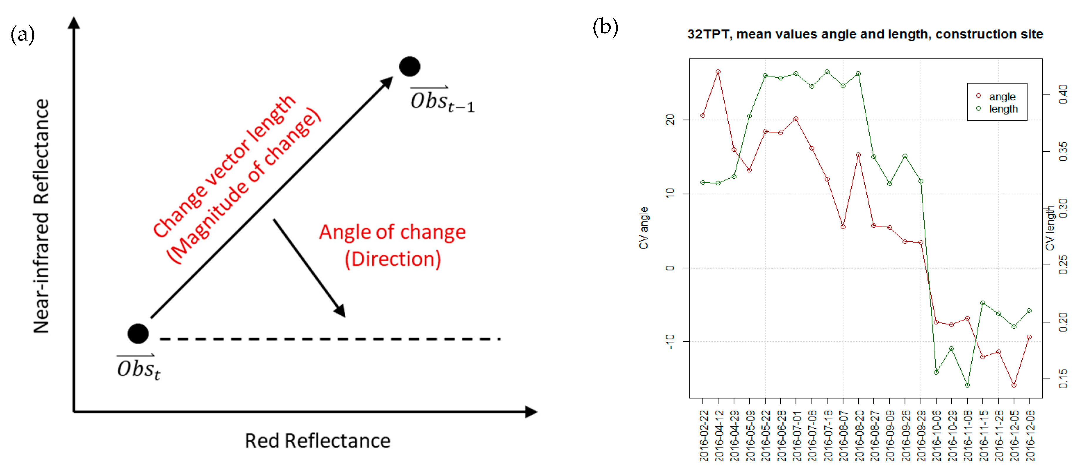
Figure 2a shows the behavior of the length and the angle of the change vector while
Figure 2b exhibits the trajectory (time series) of both measures for a typical construction site. For emerging construction sites, high values of the change vector angle are expected. For surfaces that are construction sites at two different times, we expect low to negative values of angle and length. For every monthly time step, an angle and a length pair (
t,
t1) were calculated, i.e., 2015-12 to 2016-12, 2017-12 to 2018-12, etc. Every pixel has a certain change or length-angle value (see
Figure 2b).
Based on the previously calculated CVA angles and lengths, binary change masks were then derived for each month based on statistical analysis. It turned out that the 90th percentile is a good threshold value for angle/length values to identify urban changes (i.e., a vegetation loss). Thus, each time a pixel is above the 90th percentile, a change is indicated (class 1). All unchanged areas are considered as class 0.
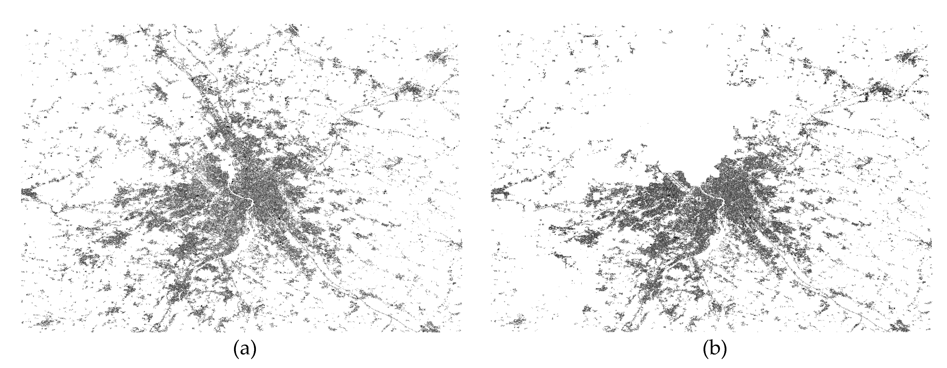
In
Figure 3, two angle value pairs are shown. As images can be affected by clouds, any parts of the image that are affected will not provide timely information and will only be updated once cloud-free observations become available through additional observations. This has an impact on the timing of the detected change.
Finally, all the binary change masks produced for each month are aggregated into monthly sums. To remove outliers and image artifacts, changes that occurred less than twice per month were removed from the mask. Additionally, to reduce confusion with agricultural fields, which typically lack vegetation cover in the winter and hence may be confused with construction, an additional layer based on the NDVI was produced to remove such false positives. Finally, a two-pixel minimum mapping unit (MMU) filter was applied to enhance the consistency of the change detection outputs. An example of a detected construction site is shown in
Figure 4. In the top, two NDVI images are depicted, showing the situation before and after construction started. In the bottom, the same construction site visualized on Google Earth imagery is shown, demonstrating the correct detection.
In the last step, one out of four possible classes (Residential, Industrial, Infrastructure and Other) was assigned to each change polygon based on a manual interpretation process using RGB images (orthophotos and very high-resolution satellite imagery) and context information from the environment surrounding the detected construction site.
This algorithm is one of several types of change detection algorithms that comprise the LandSense Change Detection Service (CDS).
4. Change Validation Methodology
This section presents the methodology used to validate the sites that were predicted to have undergone a LULC change. The validation methodology used here is founded upon the best practices for the rigorous assessment of the accuracy of land cover products [
30,
76]. The validation methodology was structured into three main steps: sampling design, response design, and accuracy assessment.
4.1. Sampling Design
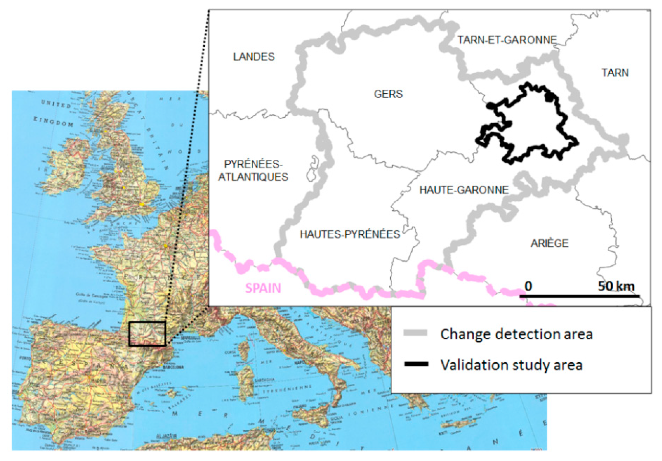
The sampling design is the protocol for selecting construction sites (i.e., changes) for use in the validation. Using Sentinel 2 imagery for the period 2015-2019, the change detection algorithm was applied to an area of approximately 10,000 km² representing three French departments: Gers, Haute-Pyrénées. and Haute Garonne (see
Figure 5).
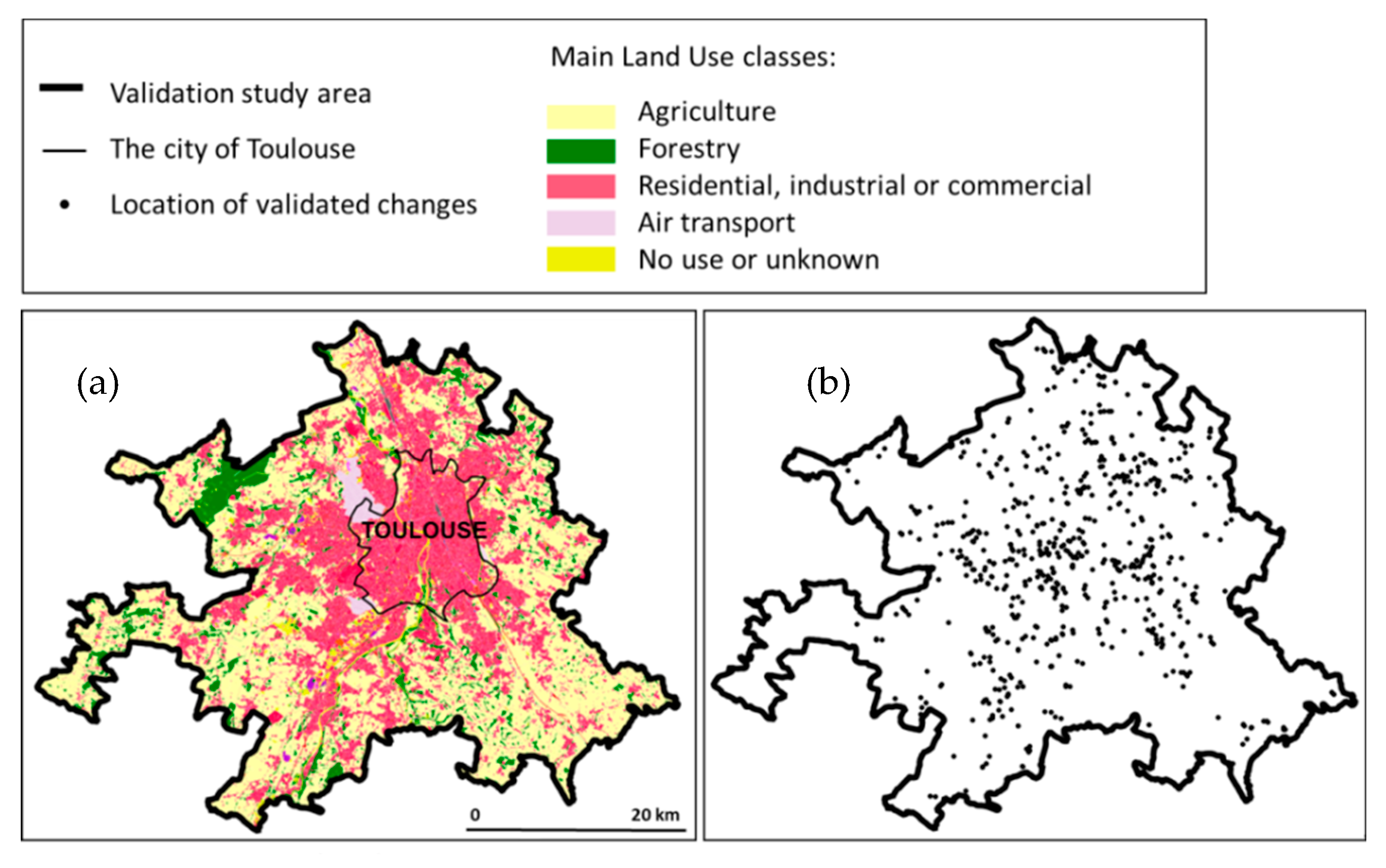
The pilot study area within the LandSense project is Toulouse and its surroundings. The overall aim was to assess the potential of updating authoritative LULC data sets with the changes obtained from the CDS, where the focus was on validating the LU changes that occurred over a specific time period. Thus, spatio-temporal sampling was undertaken of all the construction sites that were observed within the study area during the identified period of interest. The spatial limits of the validation study area were defined by the needs of the end-users and correspond to formal local authority areas (
Figure 6). The period of interest was defined by the authoritative mapping agency, here seeking to assess the potential to update a LULC database for 2016 with the situation in 2019. Consequently, the core aim was to label all the construction sites detected by the application of the CDS from 2016 to 2019 for a set of administrative units within an urban and peri-urban environment. Only the sites predicted to have undergone change within the study area in 2016-2019 were used. Note that this approach does not allow omission errors to be identified. This is a limitation of our approach, which can be managed if reference data including all changes in the test area are available.
4.2. Response Design
The aim of the response design is to define the protocol for labeling the reference data. More specifically, it defines how contributors will assign a label to the changes, which type of additional data will be used in order to allow contributors to make such a decision, and which types of additional labels should be added to reduce the confusion during the validation process.
In this study, the response design is comprised of the steps undertaken to determine an agreement between the construction sites predicted by the CDS and the reality on the ground.
The first step consists of defining the pre-defined labels to be chosen by the contributors. As mentioned in
Section 3, the outputs from the CDS represent a new construction site (e.g., a building or a road), which were then classified into four LU classes:
Residential,
Industrial,
Infrastructure, and
Other. Since some changes occur over a long time period and their final nature may not be apparent until near the end of the process, the classes
Construction in progress and
Destruction were defined and added to the list of labels defined in the response design. Additionally, since it was possible for a site to be incorrectly classified as having undergone a change (i.e., a false positive), an additional class,
No change, was defined. Finally, in recognition of the challenges in identifying a change, a site could also be labeled as
Unknown. In total, therefore, there were eight classes in the validation.
The second step consists of identifying the additional data that allow contributors to choose the appropriate label for each class. The validation of changes involved visual interpretation of fine-resolution (20-50 cm) orthophotographs for 2016 and 2019. Note that other WMS layers such as OSM and Google Maps were available in the validation tool. As a result, for each location of interest for which a change exceeding a two-pixel MMU had been predicted, a ground reference data set for change was constructed, enabling the accuracy of the predictions to be assessed.
The third step is to choose the appropriate type of validation. To avoid influencing the contributor’s validation, the interpretation of the orthophotographs was undertaken blind of the predicted change (i.e., the contributor does not know the predicted classes).
Finally, to explore the effect of inter-interpreter variations on the reference data set, validation data from six different groups of interpreters were obtained in a series of mapathons. In each mapathon, the data sets and tools were introduced to participants at the beginning, along with a summary of the project’s aims. IGN staff were also available to provide assistance during the mapathons. Each mapathon involved a different group of contributors; no mapathon had mixed contributions. The profile of each group is summarized briefly below.
Profile 1: First-year students of the National Engineering in GIS School (ENSG) who attended a brief training-event on aerial photograph-interpretation comprising a 1-hour lecture and a 2-hour training session on aerial photograph interpretation. For this group, the validation exercise was included as part of their formal curriculum in order to apply skills related to aerial photograph-interpretation. This group comprised 60 students, and while not experts in LULC data, they would have received a semester of training in geographic science. For the mapathon, this group was divided into two groups, comprising 30 students each and identified as Profile 1-gr1 and Profile 1-gr 2.
Profile 2: Students from the Master s degree in geographical information science (GIS) at ENSG. The mapathon was part of their curriculum and the data collected were used further in their practical work. These students had, as part of their curriculum, already studied remote sensing, spatial classification, and spatial data validation before taking part in the mapathon. Of the 19 students, some also had experience in aerial photograph-interpretation. However, these students are not experts in LULC data.
Profile 3: First-year students of ENSG who have not received training in aerial photograph-interpretation. This group consisted of a set of 15 student volunteers, who had begun their one-month curriculum in geographic sciences. They were motivated by gaining a better understanding of environmental applications related to LULC and the connection to research. One of the students originated from the study area. These students did not have any specific training related to LULC, image analysis or aerial photograph-interpretation and were not experts in LULC.
Profile 4: Research experts in LULC working at the research department of IGN-France. This group comprised four research experts in LULC data, map classification, and change validation. These contributors were aware of the LandSense CDS and the change detection algorithm used within it.
Profile 5: Experts in LULC from the local authorities. This group comprised five experts in LULC data from the Urban Planning Agency in Toulouse. They have good knowledge of LULC classification, aerial photograph-interpretation, and geographic data mapping, but few have knowledge of remote sensing.
Profile 6: Administrative staff from IGN. This group comprised two staff from IGN, both non-experts in LULC data or geographic data in general.
A mapathon was organized for each profile, except for those in Profile 1, where two mapathons were organized. The same data set was used in each mapathon but because of time limitations, not all sites were validated during the mapathon. The number of observations collected per profile is: 248 (Profile 1-gr 1), 195 (Profile 1-gr 2), 645 (Profile 2), 649 (Profile 3), 53 (Profile 4), 644 (Profile 5), and 344 (Profile 6).
In total, 105 contributors were involved in the mapathons, producing a total of 2778 ground reference data labels.
4.3. Quality Assessment
The final step in the validation methodology was focused on the assessment of the quality of the change detection labeling made by the contributors to the mapathons arising from the application of the CDS. The focus was on two key issues: contributor agreement and thematic accuracy assessment.
4.3.1. Contributor Agreement
The contributor agreement was assessed on an individual site basis. The goal was to assess the agreement between mapathon contributors for each site labeled. The latter was achieved using the
Pi measure proposed in the computation of Fleiss’ kappa coefficient [
77]. Based on the total number of sites labeled,
N, into one of
k classes by
n contributors and with
nij, representing the number of the contributors assigning case
i to class
j (where
j = 1, …,
k), then the proportion of all assignments associated with class
j, noted
pj, can be calculated from the following equation:
The degree to which the contributors agree on the
ith subject,
Pi, may be calculated from:
In the following, Pi is named the contributor agreement for the labeled site i.
4.3.2. Accuracy Assessment
In order to assess the accuracy of the change predictions obtained from the CDS, a single ground reference label was required for each case. Here, each case was allocated to the class that was most commonly (i.e., dominant) applied to it. If there was a tie, the case was randomly allocated to one of the classes involved in the tie. The confusion matrix was used to assess overall accuracy (OA), user’s accuracy (UA), and producer’s accuracy (PA) [
76,
78]. Overall accuracy quantifies the proportion of all sites of change that were correctly classified based on the reference data. The UA for a class quantifies the proportion of correct classifications of the class based on the reference data and indicates accuracy from the map user’s point of view. The PA for a class quantifies the proportion of correct classifications for the class based on the predictions from the CDS, and it indicates the accuracy of the classification from the map maker’s point of view.
Thus far, we used the dominant class label, but the data can be filtered to focus on cases with the least disagreement and high significance. Therefore, the confusion matrix is computed only for filtered changes by following the approach proposed in [
78].
5. Results and Discussion
5.1. Description of the Observations
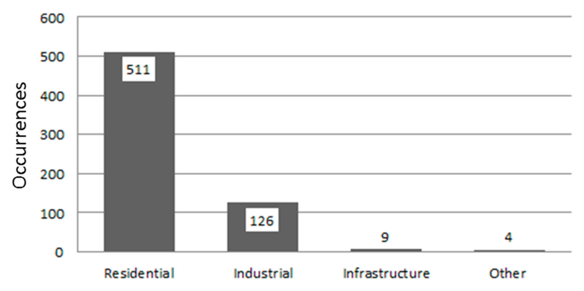
Within the entire study area (i.e., the three French departments), 650 sites were predicted as having changed land-use class during the period of interest. These 650 sites were then selected for validation in the mapathons. The most frequent changes detected by the CDS were in LU classes Residential (511 sites) and Industrial (126 sites) (
Figure 7).
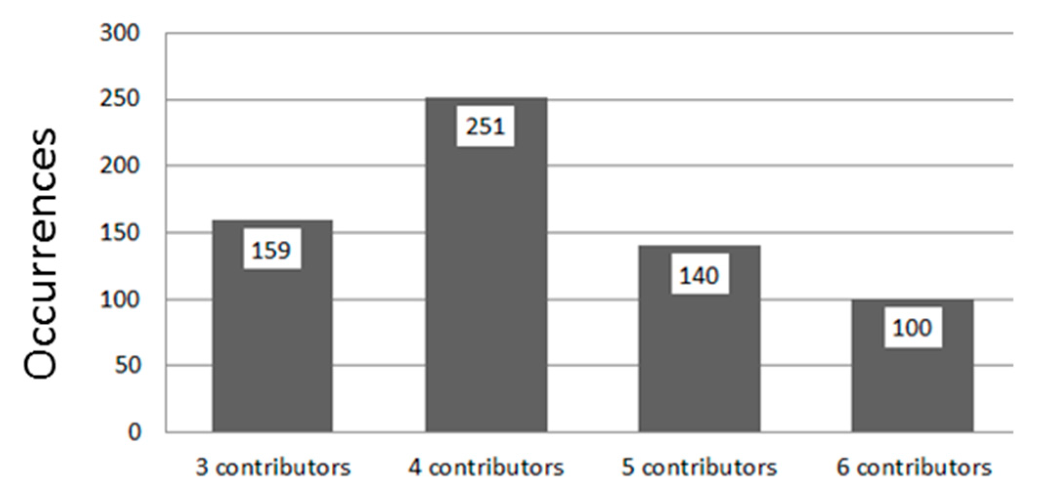
The aerial photography for these 650 sites in 2016 and 2019 was used to acquire reference data to evaluate the accuracy of the CDS predictions. Each site was labeled by between three and six contributors to the mapathons, with most sites labeled by four contributors (
Figure 8).
5.2. Contributor Agreement Analysis
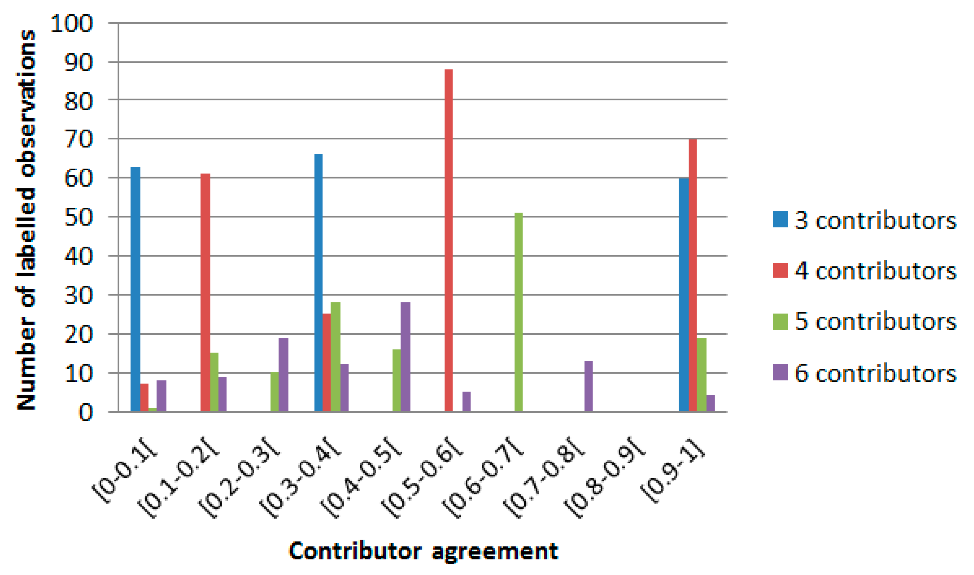
The degree to which contributors agreed in labeling sites was assessed using Equation 4 for all sites labeled by three or more contributors. All levels of agreement observed are depicted in
Figure 9. We can observe that when six contributors labeled the same site, they are in perfect agreement very few times (four labeled sites only) and that the total disagreement (contributor agreement belongs to the interval [0-0.1[) occurs mainly where sites are labeled by three contributors (63 labeled sites). In contrast, contributor agreement is high (belonging to the interval [0.9-1]) where three or four contributors label the same site. Contributor agreement belongs to intervals [0.5-0.6[ and [0.6-0.7[ for four and five contributors, respectively. Based on this analysis, we can recommend that the total number of contributors labeling the same site should be between three and five.
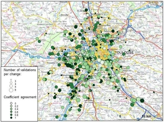
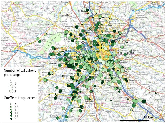
The map in
Figure 10 shows the spatial distribution of the number of labeled observations per change and the coefficient of agreement values for each site. No global trend emerges from this visualization. Indeed, the use of the Local Moran’s I statistic suggests that there is no spatial autocorrelation present except for a small area in the northern part of the study area.
5.3. Accuracy Assessement
The accuracy assessment was undertaken as described in
Section 4, taking into account the class proportion and expressed as the overall accuracy (OA). In order to focus on sites with the least disagreement, labeled sites were removed when P
i was lower than 0.4 (i.e., 176 sites removed). If a reference feature had the label Unknown, it was also removed (i.e., two changes). Thus, the accuracy assessment was computed for 467 labeled sites (71% of the total number of sites identified by the CDS).
The OA was determined to be 0.81. The user’s and producer’s accuracies are depicted in
Figure 11. We can notice that both the UA and PA are greater than 0.85 for the Residential class. This means that the CDS is appropriate for detecting residential changes. The UA for the Infrastructure class is low, being equal to 0.5. This is not surprising given the difficulty in detecting Infrastructure usage.
Most of the sites predicted by the algorithm such as
Other have an agreement less than 0.4 or have the reference label assigned to
No change. This explains why the UA and PA are equal to 0 and are, thus, not represented in
Figure 11.
Computing the change/no change confusion matrix is difficult since we do not have the reference corresponding to all changes that occurred or the location where changes do not occur. However, as a guide to changes that were not identified, during one mapathon with the experts in LULC (Profile 5), they identified 142 sites of change that were not detected by the CDS algorithm. Moreover, as a guide to the accuracy of the change detection algorithm, only the UA for the change class was computed. Thus, the reference change class is defined by considering sites in which the labels were assigned to one of the following: Residential, Industrial, Infrastructure, Other, Construction in progress, and Destruction. For example, if a reference change has the label Construction in progress, then the reference change class has the value “change”. In total, 561 sites were assigned to the reference class “change”. Thus, the UA for the change class is equal to 0.87.
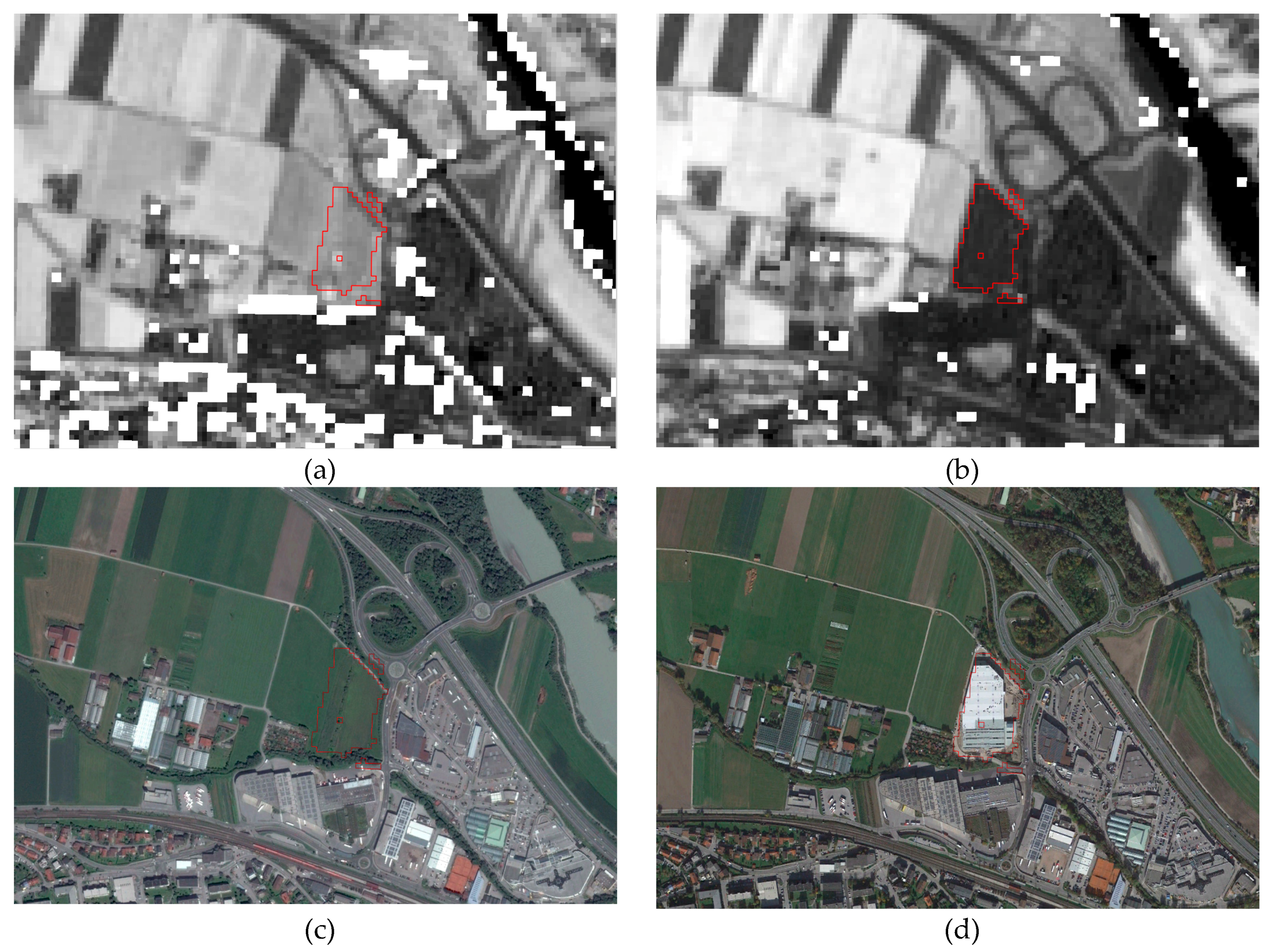
Figure 12 shows an example where both the CDS and the reference labels agree: Industrial change. The contributor agreement, P
i, is equal to 0.4.
Figure 13 illustrates the impact of scale on the validation task. The CDS detected a residential construction site and the reference value was labeled as
No change (with a contributor agreement P
i equal to 1 for three contributors). When comparing the two orthophotos from 2016 and 2019, it can be seen that a small change has actually occurred but within an area that was otherwise unchanged. This highlights uncertainty in the labeling linked to the extent of the area of change.
5.4. Profile Analysis
In this section, we analyzed the sites labeled by different interpreter profiles. As mentioned in
Section 4, the response design comprises seven labels, and contributors with six different types of user profiles were involved in the seven organized mapathons. Based on this, different research questions can be posed such as: which knowledge is necessary for undertaking a LU map validation task? Is the motivation (e.g., a volunteer task versus a mandatory task included in the curriculum) a factor that impacts the accuracy assessment?
To better assess the capacity of different profiles to carry out LU map validation, we first computed the confusion matrix between labels derived from each profile group and the reference. In total, seven confusion matrices were computed. As with the contributor agreement, only labeled sites having less disagreement were selected.
Figure 14 illustrates the overall accuracies obtained from each profile. For example, the largest overall accuracies were obtained for Profile 4 (Research experts), Profile 5 (LULC experts), and Profile 3 (volunteer engineering students). Contributors belonging to these profiles agreed with the reference of labeled changes, 93.2%, 86.5%, and 85.2%, respectively. The lowest overall accuracy was obtained when comparing Profile 1, gr2 (engineering students) with Profile 2 (students with no knowledge of photo-interpretation and LULC data) and Profile 6 (which is similar to a citizen profile with no knowledge of GIS). The very surprising difference between the overall accuracies of Profile 1 gr1 and gr 2, which are students with the same profile, can be explained by the fact that the 2019 orthophoto WMS layer was not available for a short period of time during the mapathons. Thus, for some cases, it was difficult to label the site using only Google Maps and orthophotos from 2016. We also observed that imagery in Google Maps was not updated in the study area. The lower accuracies for Profile 2 and Profile 6 can be explained by the lack of knowledge in photo-interpretation of orthophotos and in identifying changes. Finally, we can observe a relatively large difference between Profile 1, gr1 (where the mapathon was part of the curriculum) and Profile 3 (where the mapathon was a volunteered activity), and here we can observe that volunteers do better than non-volunteers.
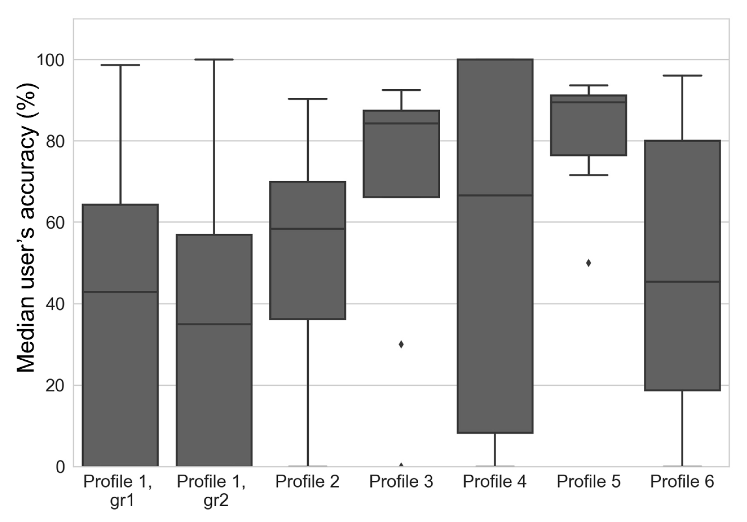
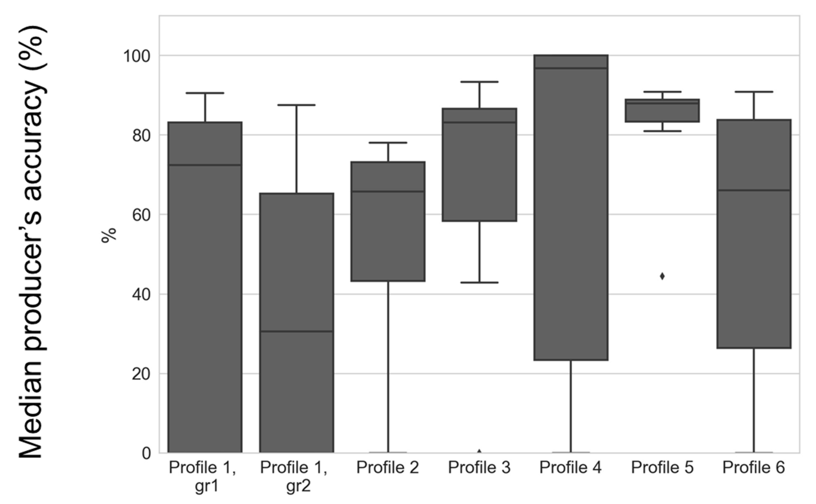
User’s and producer’s accuracies were obtained by comparing the label provided by different profiles with the reference for each possible land-use class. The results for each profile are presented using boxplots in
Figure 15 and
Figure 16 which shows the median user’s accuracy over all classes per profile.
The median values of the user’s accuracies for all profiles are generally greater than 50% except for Profiles 1 and 6. For Profile 5, the median value exceeds 90%. We can observe large variations for all profiles except for Profiles 3 and 5.
For producer’s accuracies, the median values of all profiles are generally greater than 65% except for Profile1, gr2. For Profiles 1, 2, 4, and 6, there are also relevant variations in the producer’s accuracies.
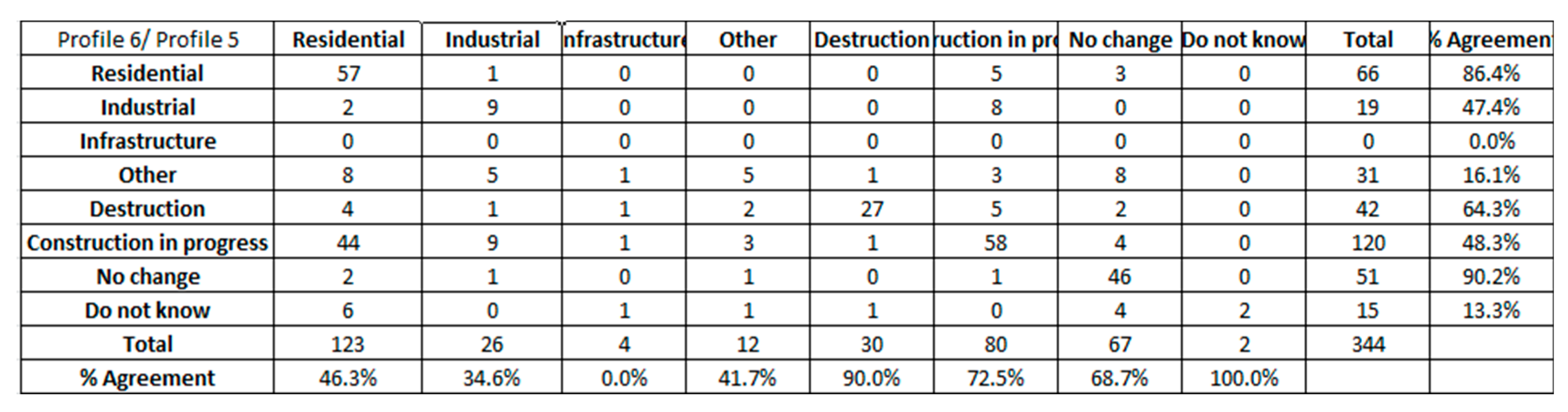
We then compared the profiles by computing the confusion matrix between pairs of profiles. Here we show the example of the confusion matrix that results when comparing Profile 6 with Profile 5 (
Figure 17).
The two profiles have a relatively good agreement for the No change and Residential classes. Small agreements are obtained for Construction in progress and Industrial. For example, 44 of the changes (36%) assigned to Residential by Profile 5 were assigned to Construction in progress by Profile 6. This is an interesting example that illustrates that the experts analyzed the spatial context even when the construction was not completely finished in order to “guess” what the LU type of construction could be. Note that these are also local experts who know the study area. Moreover, we learned that during the mapathon involving participants from Profile 5, the contributors used LULC data to interpret the change and they discussed these changes between them. Finally, a relevant difference exists for the class Unknown: 13.3% against 100%. This demonstrates that the experts tried to label each site, even when it was difficult to assign a LU type.
6. Conclusions
Change detection in urban areas is a challenging topic. This research has indicated the potential to acquire useful information on urban LULC change but enhancements are still required for operational use. Changes are detected automatically by using a method based on Sentinel-2 data. In order to assess the accuracy of the detected changes, VGI was used by organizing mapathons, employing collaborative validation tools and involving contributors with six different profiles (or backgrounds). To be able to use the changes to update IGN’s authoritative LULC database, extra classes were added to have more detailed land use classes. The profiles of the contributors were analyzed to understand the impact of the experience of the users on the accuracy assessment.
The accuracy assessment indicates that the change detection method provides promising results in detecting LU changes, with an overall accuracy of 0.81. Moreover, the method is able to identify changes in residential LU with what appears to be to an adequate level of accuracy (0.92). However, the method needs further improvement in detecting changes in infrastructure and industrial LU classes, as both users’ accuracies were low. The omission of changes is also relevant for infrastructure concerning the knowledge we have from the authoritative topographic database (i.e., the road network); the changes in the infrastructure are relevant for the period studied (i.e., 2016 to 2019). Concerning the change/no change accuracy assessment, it was, unfortunately, not possible for us to measure the omission of the change due to the lack of reference data. This issue can be tackled in the future by adding not only construction sites to the sample that have been provided by the change detection method but also other triggers coming from different VGI projects where citizens send in alerts when a change occurs [
79].
The change detection method presented here has delivered what appears to be reasonable results; nevertheless, it shows deficits in some areas. For example, information is missing when there are clouds, and there is an issue with non-existing vegetation in the winter so it is not possible to detect a change during this time. To assign a pixel to non-urban, one must wait for the next vegetation period. Before then, it is almost impossible to distinguish bare fields from urban areas. Concerning the method, future work will address problems caused by gaps due to clouds and other means for more fully capturing changes that currently go undetected. Labeled changes will be also be used to improve the change detection labels.
In terms of user profiles, we observed differences between profiles. The experts in LULC from local authorities, researchers in LULC at the IGN, and first-year students with basic knowledge of geographic information systems had the highest overall accuracies. Moreover, for profiles having the same theoretical background (Profile 1 and 3), the volunteers perform better validation than the non-volunteers. Differences in how the users approach the validation task are evident (e.g., local authorities used knowledge and context to try to identify types of change while those with no knowledge of LULC such as citizens. were quicker to choose ‘Unknown’ when the visual interpretation class became more uncertain).
From a VGI perspective, we observed that LULC data are very complex data and there are many issues related to validation. For example, LULC experts from the local authorities spent much more time in interpreting a single change; they used the metadata specification concerning LULC and discussed examples between them during the mapathon as well as with colleagues. A similar behavior, except for consultation of the metadata specifications, was noted for students participating in the volunteer mapathon. Another key issue concerns the response design. The response design (eight classes) was judged as complicated by the citizens and students without LULC experience, in contrast to the LULC experts from the local authorities, who felt that it was not detailed enough. This brings us to the conclusion that LULC validation is a very complex task, and there is no simple or obvious way to select the best group or the best response design. In future research, we would like to test a response designed based on the contributor’s profile (e.g., simplified into change/no change for the citizens and students, and a more detailed response design for the LULC experts). For the latter, discussions have already started in order to define the necessary land use classes to better fit their user needs.
The next step is to use the validated changes to update the authoritative LULC database. These data will be fused with a variety of other sources of geographic data including in-situ validation data collected during the LandSense project, and topographic data.

 ,
, 


