Monitoring of Canopy Stress Symptoms in New Zealand Kauri Trees Analysed with AISA Hyperspectral Data

Abstract

The endemic New Zealand kauri trees (Agathis australis) are under threat by the deadly kauri dieback disease (Phytophthora agathidicida (PA)). This study aimed to identify spectral index combinations for characterising visible stress symptoms in the kauri canopy. The analysis is based on an aerial AISA hyperspectral image mosaic and 1258 reference crowns in three study sites in the Waitakere Ranges west of Auckland. A field-based assessment scheme for canopy stress symptoms (classes 1–5) was further optimised for use with RGB aerial images. A combination of four indices with six bands in the spectral range 450–1205 nm resulted in a correlation of 0.93 (mean absolute error 0.27, RMSE 0.48) for all crown sizes. Comparable results were achieved with five indices in the 450–970 nm region. A Random Forest (RF) regression gave the most accurate predictions while a M5P regression tree performed nearly as well and a linear regression resulted in slightly lower correlations. Normalised Difference Vegetation Indices (NDVI) in the near-infrared / red spectral range were the most important index combinations, followed by indices with bands in the near-infrared spectral range from 800 to 1205 nm. A test on different crown sizes revealed that stress symptoms in smaller crowns with denser foliage are best described in combination with pigment-sensitive indices that include bands in the green and blue spectral range. A stratified approach with individual models for pre-segmented low and high forest stands improved the overall performance. The regression models were also tested in a pixel-based analysis. A manual interpretation of the resulting raster map with stress symptom patterns observed in aerial imagery indicated a good match. With bandwidths of 10 nm and a maximum number of six bands, the selected index combinations can be used for large-area monitoring on an airborne multispectral sensor. This study establishes the base for a cost-efficient, objective monitoring method for stress symptoms in kauri canopies, suitable to cover large forest areas with an airborne multispectral sensor.

1. Introduction

The New Zealand kauri trees (Agathis australis (D. Don) Lindl.) are a key species of New Zealand’s northern indigenous forests [1] and are of high cultural [2] and ecological significance. The conifers are threatened by the deadly kauri dieback disease (Phytophthora agathidicida (PA)). The soil-borne disease was first officially confirmed by Beever (2009) [3] in the Waitakere Ranges, although it might have been in New Zealand for decades already [3,4]. Meanwhile, it has been verified over major parts of the kauri distribution area [5]. To date, the monitoring of kauri dieback symptoms has relied on fieldwork and the manual interpretation of aerial images and photos taken from aircraft and helicopters [6,7]. There is a need for a cost-efficient, objective approach for the monitoring of stress symptoms which allows for the coverage of large areas [8].

1.1. Kauri and Kauri Dieback Disease

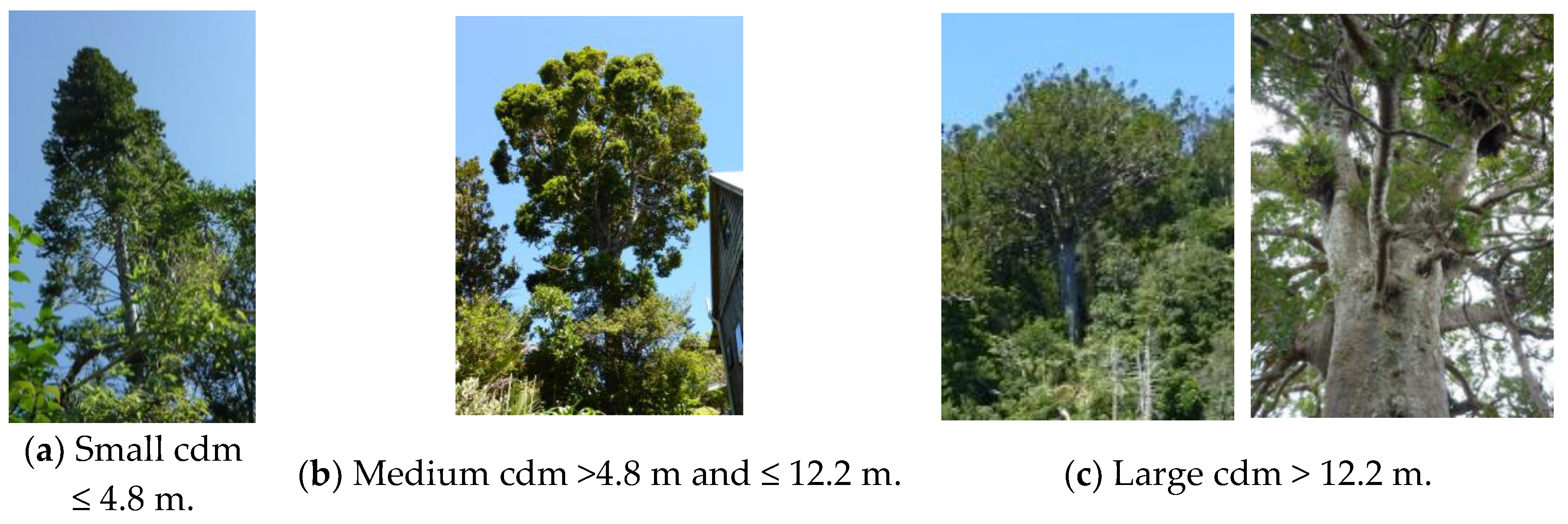
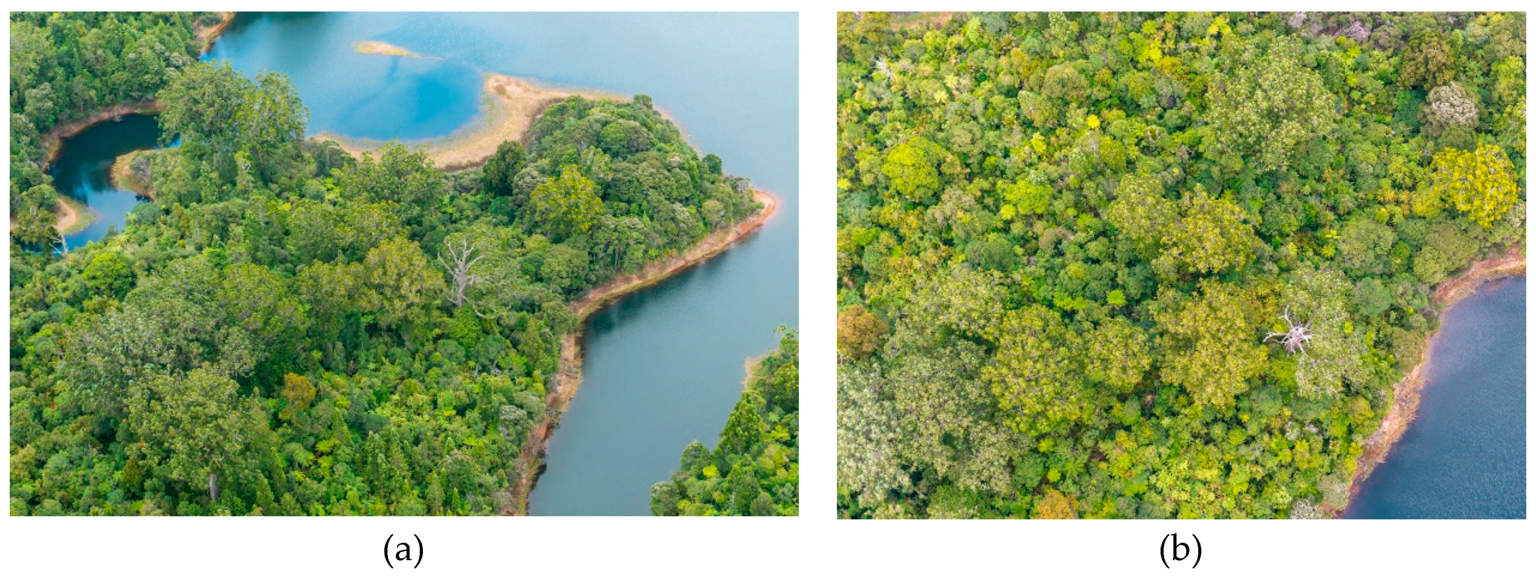
The New Zealand kauri is an endemic conifer with a natural distribution in the upper North Island. The existing stands of mature kauri are what remained from extensive logging by European settlers in the 19th and early 20th centuries [9]. Young kauri have a small conical shape with dense foliage. Older kauri emerge over the surrounding vegetation and develop a massive trunk and a large dome-shaped crown [10] with measured diameters of over 30 m and heights of up to 40 m in the study areas. The lanceolate leaves of kauri are broad needle-shaped, ca. 2 to 5 cm long, with a smooth leather-like surface [10] and form a spiky foliage surface. While the foliage of small kauri is dense and evenly spread over the crown, the leaves of medium and large size kauri are arranged in clusters (Figure 1) which expose gaps, shadows and visible branch material, even in the non-symptomatic stages. The kauri foliage occurs in colour variations from darker yellow-green to lighter blue-green (Figure 2) [10].

Infection with PA causes lesions in the trunk and roots, which block the transport of water and nutrients [1,3]. The first visible signs in the canopy are yellowing of the leaves and leaf loss in the top of the crowns, which exposes bare branches. In some crowns, the symptoms impair only parts of the upper crown if the transport system is partially blocked. With progressing decline, the foliage becomes sparse, bare branches become exposed, and the influence of woody material, internal shadows, visible undergrowth and ground litter in the canopy reflectance increases. Weakened kauri are less effective in shedding off climbers and epiphytes, which, again, add green plant material in the canopy. In the final stage, the remaining foliage turns brown before it falls off and small branches drop until only a bare skeleton remains. Dead and dying kauri trees are again quickly overgrown by undergrowth, neighbouring trees, epiphytes and climbers.

A variety of factors can accelerate the progress and intensify the symptoms of an existing PA infection, including drought conditions, difficult growing conditions on shallow soil and the exposition to strong and salty winds from the sea. These factors alone and also infections with other pathogens, e.g., Phytophthora cinnamomi [4,14], can cause similar canopy stress symptoms.

1.2. Remote Sensing for Stress Monitoring

Various authors have found that there is a good relationship between spectrally derived indicators extracted from remotely acquired optical imagery and stress symptoms in tree canopies caused by forest diseases [15,16,17,18,19,20,21].

Airborne hyperspectral images have been used successfully in many studies to analyse tree canopy health in conifers [22,23,24,25,26,27] and broad-leaved species [28,29,30]. The full spectral range allows for the processing of a spectral continuum and the identification of important bands from a large range of narrow bands [31] that are sensitive to subtle reflectance changes for early stress detection [32,33,34]. However, high costs for the data acquisition and maintenance of the sensors, elaborate calibration and processing, and small swath widths qualify airborne hyperspectral sensors for the time being more for analytical research tasks than regular large-area forest monitoring.

Spaceborne imagery is the most cost-efficient option to cover larger areas, as it is comparably easy to process and has been widely used to monitor stress responses in tree canopies [35,36,37,38,39,40,41,42]. However, satellite images often lack the spatial and spectral resolution for an assessment on the individual tree crown level and are bound to certain over-flight times [19,39]. Acquisitions with crewed aircraft are a more expensive option than satellite imagery but provide a more flexible timing and higher spatial and spectral resolutions. Unlike unmanned aerial vehicle (UAV) sensors [43], multispectral sensors for crewed aircraft are well suited to large-area coverage with a large swath width, a low noise-to-signal ratio and a robust sensor setup [44,45,46,47]. However, the spectral limitation of multispectral sensors to usually four to six bands requires previous knowledge about the best band combinations to detect the target features. The approach in this study combines the strengths of both the hyperspectral and multispectral platforms. We utilized the high spectral resolution imagery from a hyperspectral sensor to define band and index combinations that are suitable to be mounted on a multispectral sensor on a crewed aircraft for large-area stress monitoring in kauri canopies. The spectral ranges used in this study are defined in

Table 1. Spectral ranges with wavelengths used in this study (adapted from [48]).

Spectral Range	Electromagnetic Wavelengths
Visible (VIS)	437–700 nm 1
1st near-infrared (NIR1)	700–ca. 970 nm 2
2nd near-infrared (NIR2)	970–1327 nm
1st shortwave infrared (SWIR1)	1467–1771 nm 3
2nd shortwave infrared (SWIR2)	1994–2435 nm 1,3

¹ The useable bands of the AISA Fenix image with low noise levels covered the range between 437 and 2435 nm. ² The upper band of NIR1 range marks the shift between the two sensor parts at 970 nm. ³ The transition from the NIR to SWIR1 and from SWIR1 to SWIR2 regions is marked by atmospheric water absorption regions.

.

Vegetation indices (VI) for stress monitoring usually combine bands that are sensitive to the stress parameter(s) with insensitive bands [49]. An ideal VI for stress analysis shows a linear relationship with the targeted symptoms, is equally sensitive for all levels of stress, independent of the scale, and shows minimal saturation effects [19,50]. VIs were developed for all levels of stress from the first, even pre-visible, reactions on leaf level to obscured canopies of dead crowns.

Pre-visible stress reactions in tree foliage have been successfully detected with thermal sensors [51,52] and narrow optical bands in the visible (VIS) part of the spectrum [53,54,55,56]. The first stress symptoms are often a reaction to leaf pigment alteration and reduced canopy water content. VIs that provide a direct measure for canopy water content, like the Moisture Stress Index (MSI) [57], the Normalized Difference Water Index (NDWI) [58] and the Water Band Index (WBI) [59], are based on water absorption bands in the near-infrared (NIR) and shortwave infrared (SWIR) regions. The yellowing of leaves as an early stress symptom is related to biochemical changes in the pigment concentrations, especially leaf chlorophyll [60]. Absorption coefficients of chlorophyll are strongest in the blue and red region, around 450 and 680 nm, respectively, where green leaves absorb more than 80% of incident light [61]. While indices in these bands ”saturate” rapidly, Gitelson (2003) [61] found that ratios with narrow bands in the green and early red-edge regions are more sensitive to changes in chlorophyll, also at higher chlorophyll concentrations.

So-called “greenness” indices describe the reduction in chlorophyll based on its absorption in the red spectrum in combination with bands in the NIR region around 850 nm that are influenced by strong photon scattering in leaf air–cell–wall interfaces [62,63]. Since these indices are correlated to the amount of photosynthetic active material, they also capture a reduction in leaf area and changes in leaf angle and thereby, structural changes in the canopy [50,61,63,64]. Increased stress leads to a decline in red absorption and a narrowing of the red absorption region, which again causes a blue shift of the red-edge point. The red-edge region is very responsive to changes in chlorophyll content [61,65,66]. Narrowband index combinations with red-edge bands have been successfully used to detect early signs of water stress [67], dying material in Pinus radiata [44] and early stress symptoms in conifer woodland [66]. Further indicators of plant stress include a relative increase in carotenoid pigments and a reduction in leaf nitrogen content, which can be detected with indices that contain characteristic absorption bands in the blue region (445 nm) for carotenoids [68] and 1510 nm for protein-bound nitrogen [69].

Higher amounts of visible dry litter and dead branches are expressed by subtle reflectance characteristics of cellulose and lignin in the SWIR regions [70]. However, these characteristics are easily obscured by water absorption features and require dry conditions for the most accurate results [62,69,71]. Several studies found a close relationship between bands in the NIR and SWIR region and structural changes in the canopy due to foliage loss [72,73]. Although these relationships are non-linear and therefore difficult to interpret [64], indices in the NIR and SWIR regions were successfully used by Schlerf et al. (2005) [74] to estimate the Leaf Area Index (LAI) in Norway spruce forests.

The reflectance characteristics of conifers—like a higher absorption, lower transmittance and higher backscattering—are most distinct in the NIR bands [70]. A high optical depth in the NIR spectral region allows a maximum interaction of photons with crown elements in the lower canopy. It thereby enhances the influence of woody material and understory vegetation [57,75].

When upscaling from leaf-scale responses to crown-scale, a range of crown characteristics need to be taken into account, such as foliage condition, canopy structure, the influence of non-photosynthetic branch and stem material, epiphytes and climbers and, depending on the gap fraction, understory vegetation, soils and ground litter as well as illumination conditions, viewing geometry and reflectance from neighbouring trees [48,75,76]. These attributes have different cumulative effects depending on the spatial scale, such that successful indices at leaf-level often show lower performance at crown level [77,78]. Several studies proved that leaf optical properties play only an inferior role in reflectance on canopy scales unless the foliage is dense with a more horizontal orientation and a high Leaf Area Index (LAI) [75,79,80].

1.3. Approach and Objectives

A method for the detection of kauri trees with indices in the VIS to NIR2 range has already been presented in Meiforth et al. [11]. This study focuses on the spectral analysis of stress responses in kauri crowns over the full hyperspectral range (437–2435 nm). The aim was to identify the best index combinations that are suitable for large-area stress monitoring with a multispectral sensor.

To account for the spectral characteristics on crown level and the assessment scale of whole crowns in the reference data, we use a crown-based scale for the analysis of canopy stress symptoms over the full spectral range from visible to shortwave infrared. We chose to use a combination of indices rather than one single index to account for the wide spectral range of stress symptoms and phenological characteristics of kauri in different growth and stand situations.

With regards to the practical implementation, we pay special attention to the performance of the recommended multispectral setup for kauri detection in the context of stress detection. And we also explore index combinations in the VIS to NIR range up to 970 nm (VNIR1), which are easier to realize on a multispectral sensor. A pixel-based application of the developed crown-based model was also tested for a more fine-scale prediction of stress responses, especially in larger crowns.

The objectives of this study are to:

(1).

Identify the best band and index combinations to detect stress symptoms in kauri crowns for both the full spectral range (VIS–SWIR) and the VNIR1 spectral range. The selected band-combinations should not exceed six wavelengths, to be suitable for a multispectral platform.

(2).

Test the performance of a pre-defined band combination for stress detection, which was defined in Meiforth et al. (2019) [11] to locate kauri trees.

(3).

Test the performance of the model and indices-selections that was developed on mean crown values in a pixel-based approach by calculating the model on indices raster.

To support objective 1, we analysed the inner- and intra-crown spectral variability and described the spectral characteristics of kauri crowns for different crown size classes and stress symptom stages from non-symptomatic to dead.

This study addresses symptoms of stress in the canopy that can be caused by PA, but they can also have a range of other causes, such as drought, insect damage or other diseases. Proof of a PA infection still requires systematic soil sampling and analysis in the laboratory [81].

2. Materials and Methods

2.1. Study Area

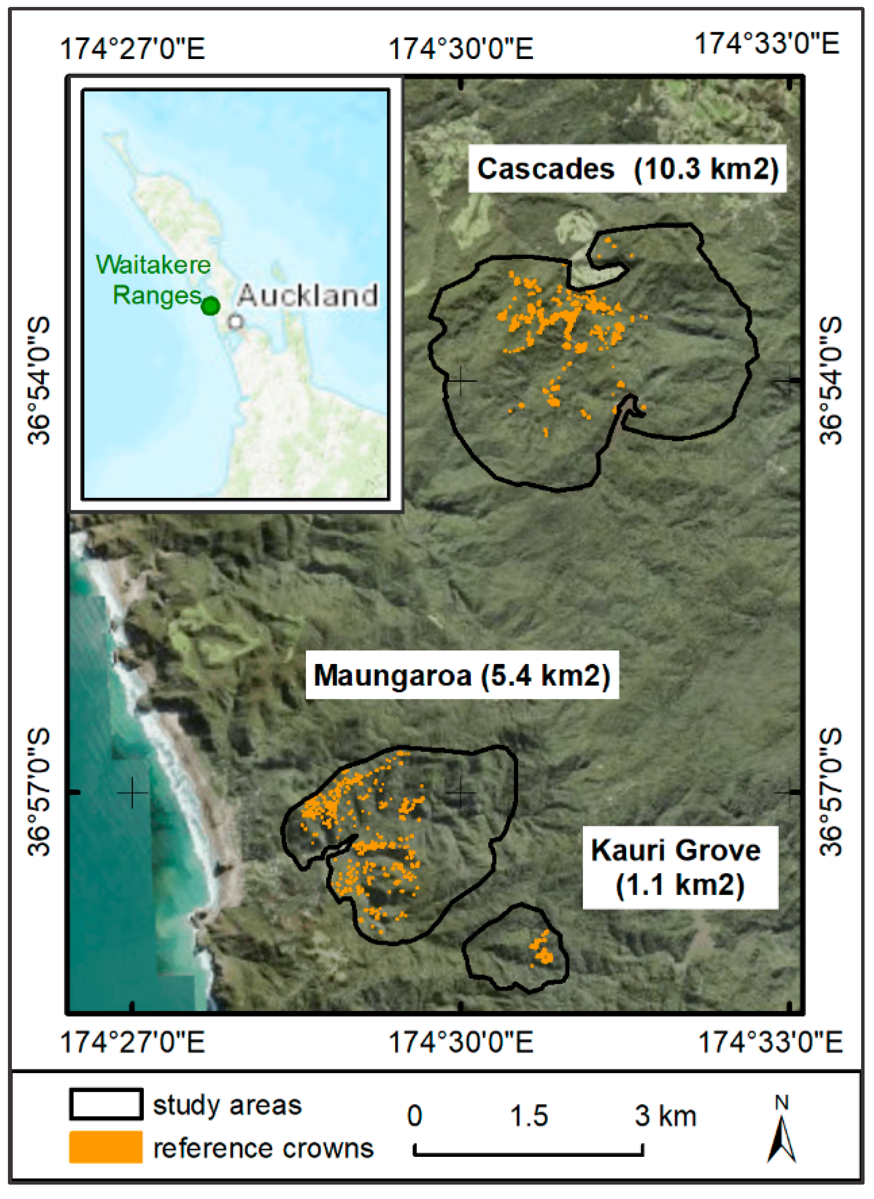
The study area is located in the Waitakere Ranges, northwest of central Auckland, close to the West Coast. The area has a warm-temperate climate that is influenced by the adjacent sea [82], and rough terrain. The three study sites cover a total area of 1680 ha with 1258 sampled reference crowns (Figure 3). The sites contain a representative range of kauri stands in all stages of stress, from younger second-growth forests in the Maungaroa area to the remains of mature kauri stands with associated tree species in the Cascade area and Kauri Grove Valley (Figure 3).

2.2. Remote Sensing Data and Preparation

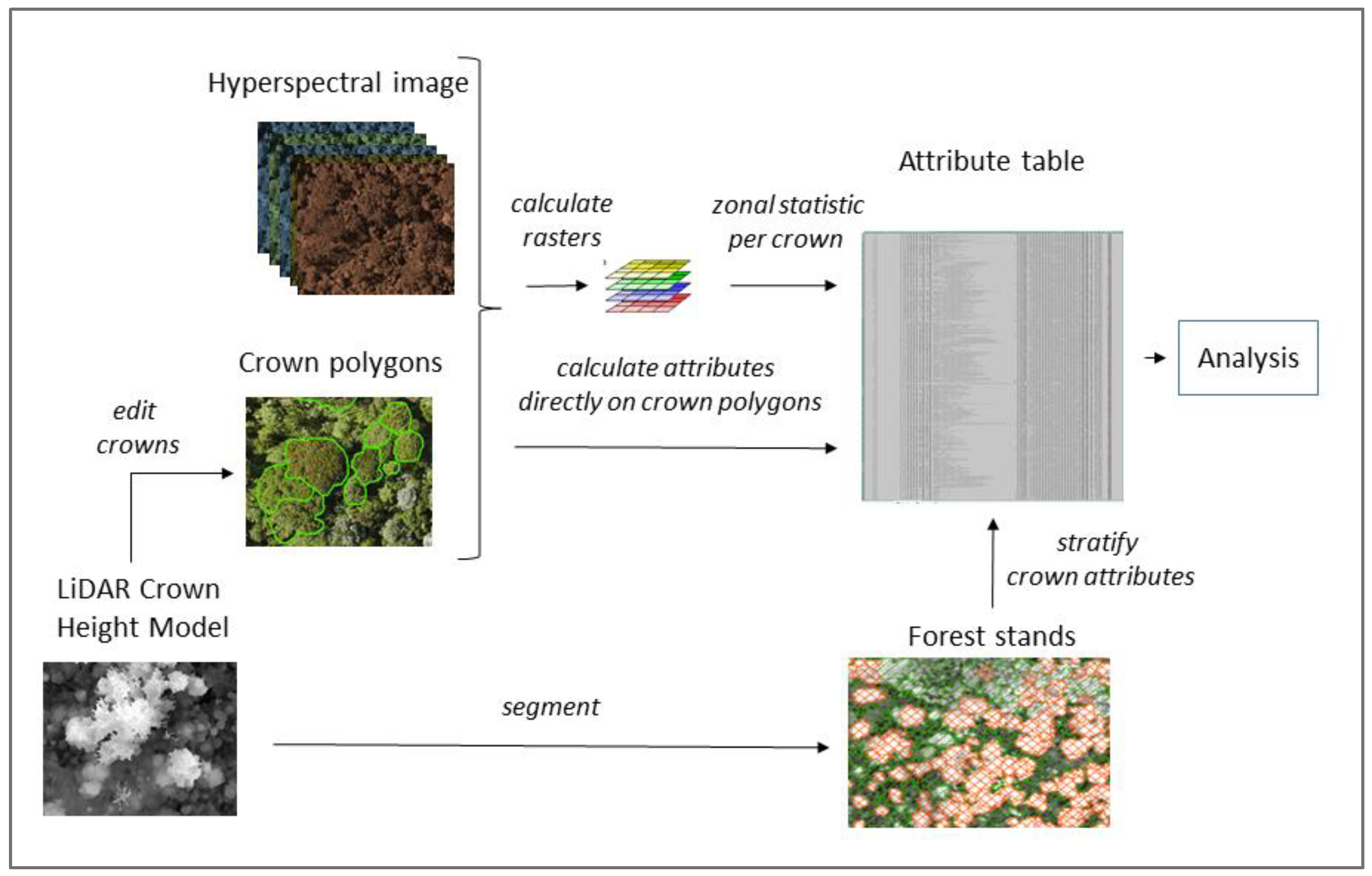
Figure 4 provides an overview of the workflow for the data preparation. We used a Crown Height Model (CHM) generated from LiDAR data to locate and edit the crown polygons for the reference crowns that were sampled during the fieldwork. Crown based attributes were calculated as zonal statistics either directly on the hyperspectral image or on (indices) raster that were derived from the hyperspectral image. The attributes were stratified according to the crown size and forest stand situation.

The analysis of kauri stress detection is based on an airborne hyperspectral image flown with an AISA Fenix hyperspectral sensor by Massey University on 15 March 2017. The original image was delivered in 24 stripes in radiance values with 448 bands from the visible to SWIR range at 1 m pixel resolution. The sensor features narrow bandwidths of 3.4 nm, on average, in the VNIR1 and 10 nm in the NIR2 to SWIR2 part of the spectrum (Table 1). The image processing included a geographic correction in Parge [85], a de-striping, an atmospheric correction in ATCOR 4 [86], an orthorectification with over 2300 ground control points in ERDAS IMAGINE, the removal of noisy bands and the creation of a seamless mosaic in ArcGIS and ENVI. The processing steps are described in more detail in Meiforth et al. (2019) [11]. The final mosaic has a selection of 352 bands and covers a total area of 9 km² over the three study sites.

Spike free terrain, surface and crown-height models (DTM, DSM and CHM) [87] were created according to a method described in Khosravipour et al. 2016 ([87]) with LAStools ([88]). The creation of height models is based on a set of LiDAR data flown with a RIEGL LMS-Q1560 sensor on 30 January 2016 by AAM NZ Ltd., with 35 returns/m² on average (0.5 ground returns/m²) [87]. The LiDAR point cloud was delivered with the ground points already classified. For the generation of the height models, we filtered out the class 7 “noise”, but kept all other points.

Two sets of Red-Green-Blue (RGB) aerial images served as a reference to assess the canopy stress symptoms in combination with field observations. One RGB image was acquired on 30 January 2016 with a 15 cm pixel size on the same flight as the LiDAR data [89]. It was delivered in two versions—orthorectified on the DTM and on the DSM. The second set of RGB aerial images with a higher spatial resolution of 7.5 cm was flown on the 2nd and 3rd of May 2017 [90]. It was delivered in an orthorectified version on the DTM so that high crowns and crowns on steep slopes were partly displaced compared to the correct position on the LiDAR CHM.

2.3. Reference Crowns

The locations of the plot areas were pre-selected based on an existing vegetation map [91], aerial images and a LiDAR CHM to provide representative coverage of terrain and growth conditions, tree sizes and symptom stages. The recorded numbers and attributes of kauri crowns were evaluated regularly during the fieldwork to ensure a balanced distribution of growth and symptom classes in the reference data set.

Two methods for locating reference crowns in the field were used, depending on the stand situation. In closed dense stands, the crowns were located in circular sampling plots of 20 and 30 m diameter with distance and bearing to a centre point, which was positioned with a mapping grade GNSS (Trimble-GeoXH-3.5G, Trimble Geospatial NZ). In combination with the recorded cardinal crown spread in the field, it was possible to accurately position the resulting crown pattern on the LiDAR CHM, which served as the main spatial reference. In more open stands, where it was possible to identify single crowns in aerial images, the crown locations were directly edited in the field as point locations on a field tablet, so that the crown polygon could be delineated afterwards on the LiDAR CHM. Some dead trees were directly identified in the aerial images. While all reference crowns with foliage were identified as kauri, in the category of dead trees, especially in the smaller sizes, it was not always possible to distinguish the species.

The polygons for each reference crown were edited on the LiDAR CHM. A buffer of 10% of the crown diameter was removed from the outer edge to avoid edge effects. The core shadow areas were removed based on a brightness threshold on the average of RGB-NIR bands. To avoid the effects of mixed pixels with the 1 m pixel size only crowns with a mean diameter larger than 3 m were used for this analysis. The final reference set includes 1258 crowns with a total sunlit area of 56,629 sqm. The crowns were sorted into three size classes according to their growth forms and average crown diameter (Figure 1).

Table 2. Overview of stress symptom classes in the reference crowns per size class according to the mean diameter.

		Stress Symptom Class 3					Total
		1	2	3	4	5
Crown Size Class 1	large	34 2	249	17	19	12	331
	medium	23 2	374	44	42	66	549
	small	61	176	35	48	58	378
total		84	833	96	109	136	1258

¹ Crown size classes according to mean crown diameter: (small = 3 to ≤ 4.8 m, medium= 4.8 to ≤ 12.2 m and large >12.2 m diameter), ² Large and medium crowns that were non-symptomatic with a dense foliage, but a more open canopy than smaller crowns, were noted with the value 1.5 in the analysis. ³ Stress symptom classes were defined from 1 = non-symptomatic to 5 = dead (see assessment scheme in Appendix B).

shows the distribution of crown size classes per symptom class, which reflects the crown situation in the study areas, with most of the crowns classified as symptom class 2 and more medium crown sizes (549) than smaller (378) and larger crown sizes (331).

2.4. Field Attributes and Stress Assessment

The recorded attributes in the field included the stem position, the cardinal crown spread, the stem diameter at breast height [92], the canopy base height, an estimated crown density and a foliage coverage according to the “Foliage Cover Scale” in DOC 2014 [93]. Optical characteristics like the yellowing of leaves and anomalies like epiphytes or double stems were noted, and each recorded kauri was documented with a canopy photo. Dead branches were documented in six percentage classes according to an index developed by the Department of Conversion [93]. The field staff assessed an overall classification of stress symptoms in the canopy from 1 = “non-symptomatic” to 5 = “dead”, corresponding to the classification scheme of Auckland Council (Figure A1 in Appendix A). Experienced staff ensured that the field reference data were comparable to the surveys of the previous years.

The final assessment of stress symptoms was based on an evaluation of visible stress symptoms on RGB aerial images from 2016 and 2017. Deviations from the overall field score were reviewed in more detail by assessing the particular field attributes and canopy photos. To secure an objective and coherent assessment, we developed an assessment scheme for the interpretation of visible stress symptoms on RGB aerial images (

Table A1. Assessment scheme for stress symptoms in kauri crowns based on RGB aerial images [89,90] for five canopy stress symptom classes and three crown sizes.

Symptom Class	Description	Size Small 1	Size Medium 1	Size Large 1
Value 1—No Symptoms	Leaves: green, green/blue; Canopy density: dense, no to small gaps; Bare branches: <1%
Value 2—First Symptoms/Open Crowns	Leaf colour: green to yellowish; Canopy density: small gaps; Bare branches: 1 to 5% (small branches)
Value 3—Medium Symptoms	Leaves: green with yellow or brown; Canopy density: small to medium gaps visible; Bare branches: 5%–30%
Value 4—Severe Symptoms	Leaves: yellow-green to brown, Canopy density: sparse, many gaps, understory partly visible Bare branches: >=30% visible as linear structures Epiphytes and climbers possible
Value 5—Dead Trees	Leaves: dead, brown leaves possible Epiphytes and climbers possible Canopy density: Gaps and understory visible, Bare branches: 100% dead branches, visible as linear structures

¹ The crown size classes are defined according to their mean crown diameter, see Figure 5. Non-symptomatic large and medium crowns with open canopies were given the value 1.5 in the analysis.

in Appendix B). It takes into account the leaf colour from green, through yellowing, to browning, visible foliage gaps and bare branches. Class 1 describes closed green foliage without visible gaps or branch material and only applies to smaller and some medium kauri sizes. For large and medium kauri crowns that do not show any signs of stress, but still feature a higher number of gaps and visible branch material, we applied the value 1.5.

2.5. Calculation and Selection of Crown Based Attributes

The mean spectra of kauri crowns in different size and symptom classes, and their standard deviations, were calculated in ENVI from the selected sunlit parts of the crowns.

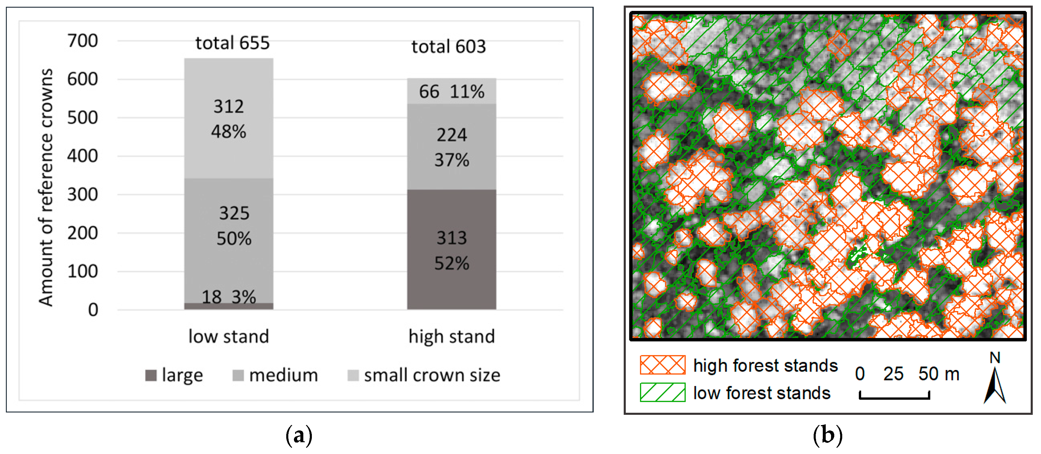
A height threshold of 21 m was defined to distinguish “high” and “low” forest stands, which were automatically segmented on the LiDAR CHM in eCognition (scale 15 m, shape 0.3 and compactness 0.9 [94]). Figure 5 illustrates that high forest stands contain a greater number of large (52%) and medium (37%) kauri crown sizes, while low forest stands feature mainly medium-(50%) and small (48%)-sized kauri crowns, with the occasional single large crown (3%).

The aim of the attribute selection was to identify a set of wavelengths and derived indices with a high correlation to the stress symptom classes. The indices should be based on no more than six bands in total and be efficient in bandwidths of at least 10 nm, to match the requirements for multispectral airborne acquisitions.

The initial selection of 95 indices for the whole spectral range was based on the selection of indices for forest health evaluation in ENVI [95] and the EnMAP toolbox [96] and supplemented with indices from the literature review on VIs summarised previously. The indices were calculated as raster images on the 352 selected hyperspectral bands that were resampled to 10 nm bandwidths with the “Spectral resampling tool” in ENVI. In noisy areas of the spectrum, the three neighbouring bands were averaged. The wavelengths of some indices were slightly modified to reduce the number of required bands for the final index selection. These indices are marked with a prefix “m” in

Table A2. Vegetation indices (VI) for the selected index combinations. The combinations cover both the full spectral range (VIS-SWIR2) and only visible to near-infrared bands (VIS-NIR1) and crown sizes from small (S) over medium (M) to large (L) crown sizes (see details in Figure 1).

Index	Equation 1	Literature	Name, Association	VIS-SWIR 2				VIS-NIR 2
Abbr. 1				all	S	M	L	all	S	M	L
LIC2	= 440/690	[109]	Lichtenthaler Index (light use efficiency)							x
BGI	= 450/550	[110]	Blue Green Pigment Index (leaf pigments)	x
PRI	= (531 − 570)/(531 + 570)	[137]	Photochemical Reflectance Index (light use efficiency)					x	x
MLO	= 531/645	[111]	M. Locherer Chlorophyll Index (light use efficiency)								x
mRGI	= 685/550 (original: 690)	[110]	Red-Green Pigment Index (leaf pigments)		x			x
NDVI-H	= (800 − 670)/(800 + 670)	[138]	Normalized Difference VI–Haboudane (chlorophyll, LAI)	x		x				x
SR670_800	= 800/670	[139]	Simple Ratio 800/670 Ratio VI (chlorophyll, LAI)	x
mSRa 675,700	= 675/700 (original 672, 708)	[112]	Simple Ratio (chlorophyll, carotenoids)				x
mNDVI-A	= (900 − 685)/(900 + 685) (original: 680)	[120]	Normalized Difference VI–Aparicio (Broadband Greenness)					x	x		x
GM2	= 750/700	[122]	Gitelson and Merzlyak Index (chlorophyll content)					x
mRVI	= 750/680 (original: 745, 645)	[108]	Ratio VI (chlorophyll content)					x
MSI	= 1600/820	[57]	Moisture Stress Index (canopy water)				x
WBI	= 900/970	[59]	Water Band Index (canopy water)					x	x	x	x
LWVI2	= (1094 − 1205)/(1094 + 1205)	[121]	Leaf Water VI (leaf/canopy water)	x	x
NDNI	= (1510 − 1680)/(1510 + 1680)	[69]	Normalized Difference Nitrogen Index (leaf nitrogen)	x	x	x
mSWIRVI	= 37.27 × (2210 + 2090) + 26.27 × (2210 − 2090) − 0.57 (original: 2208)	[125]	Shortwave Infrared Green VI (cellulose/dry matter)	x		x	x

¹ “m” indicates that wavelengths had been slightly modified compared to the cited literature. The changed wavelengths are marked in italic, and the original wavelengths are noted in italic under the equation. ² see Table 1 for the range of wavelengths in the spectral regions.

in Appendix C.

All the resulting index rasters were normalised from 0 to 1 with a linear transformation. The mean index values of the sunlit crown parts were calculated with a zonal statistic tool in QGIS. The analysis was performed on the aggregated mean crown values, to match the crown-based reference data. Highly correlated indices were removed by keeping indices with fewer bands. A first subset was defined by combining the results of a wrapper-, a classifier- and a correlation-based feature subset selection in WEKA [97]. The further selection process was based on a take-one-out method with a Random Forest regression in 10-fold cross-validation under consideration of the best correlation and attribute importance for a maximum of six bands. The selection process was repeated with indices only in the visible to NIR1 spectral range (437 to 970 nm) and for individual crown size classes.

2.6. Selection and Parameterisation of the Algorithms

Following other studies on tree health assessment [28,98], we applied a regression approach to analyse the continuous stress symptom responses in kauri crowns. The predicted range of values from a regression analysis is better suited to match the gradually declining symptoms in the forest crowns than nominal categories. There is a lot more information in the spectral indices than a 5-step reference scheme can capture and the regression approach enables to better utilize this information. The continuous range of output values in a regression helps to improve the distinction of first stages of decline, which are of special interest for the management and to account for the spectral differences in the different growth stages.

We compared the performance of six regression models in WEKA (Random Forest, Reduced-Error Pruning Tree, Random Tree, Decision Stump, k Nearest Neighbour and Elastic Net) in a 3-fold random split of all reference crowns in 1000 repetitions, by calculating the correlation coefficient with standard deviations. The Random Forest (RF) regression performed best.

The RF algorithm creates a large number of decision trees from bootstrap samples and predicts the mean value of the individual trees [99]. RF models are robust against outliers in training data, can handle a wide variety in the reference data and produce high correlations between the predicting variables [100]. They do not have requirements for the data distribution and do not tend to overfit [101,102]. We parameterised the model to a depth of 8 and set the number of iterations to 300 according to the learning curve for an out-of-bag accuracy. However, the resulting algorithm was still rather complicated—a maximum tree depth of 8 resulted in a regression tree with 199 nodes.

For an easier application, we also calculated a linear regression (LR) and M5P regression in WEKA. While the RF model requires a file to be transferred to other datasets, the resulting models of the M5P and LR can be plotted as an equation, which can be directly applied to new data. The LR is a simple parametric statistical model that is fast to train. The WEKA implementation estimates coefficients for a line or hyperplane to fit the training data by reducing the complexity of the learned model with a ridge regularisation technique [103]. However, the LR works best with a linear relationship between the criterion and predictor variable. The M5P regression in WEKA combines several linear regression models in a tree-based structure, a method that is better adapted to non-linear relationships and can handle tasks with a high dimensionality [104]. Based on a systematic test, we pruned the M5P decision tree to a minimum number of 50 instances allowed at each node.

To account for the different assumptions of the RF, M5P and LR models and deviations in the reference scheme from an ideal linear relationship with equal variances, we only used the correlation value to train and compare the models. The mean absolute error (MAE) and the root-mean-square error (RMSE) were used to compare different test setups within one model, not between the different models. We also tested a rescaling of the reference values, to establish a more linear relationship between the results and reference values for an easier interpretation of the predictions.

2.7. Test of Pixel-Based Application

According to the scale of the crown reference data, the development of the model to predict canopy stress symptoms was based on mean crown values. However, a crown segmentation is elaborate and introduces additional mistakes [105,106,107]. An area-based method would be easier to apply and enable the use of predefined kauri locations from Meiforth et al. (2019) [11] as a mask for further stress analysis. Moreover, the resulting pixel-based map gives a more representative description of partly declining crowns. The results can still be aggregated in a crown- or stand-based manner afterwards if needed. To test the pixel-based application, we applied an RF regression on the raster images of the chosen index combination for the full spectral range and compared the resulting stress index values visually with the values of the reference crowns and the RGB aerial images.

3. Results

3.1. Inter- Versus within Crown-Variability

The spectra of non-symptomatic kauri crowns are described in detail in Meiforth et al 2019 [11]. Figure 6 shows that the variability of the reflectance values between different kauri crowns (a, b) exceeds the maximum variability of reflectance within single kauri crowns (c, d). expressed by the standard deviation per crown. The unit less reflectance values were multiplied by 10000. Large and small crowns show overall the same reflectance patterns, with low separabilities in all spectral regions (

Table A3. Comparison of the spectra for small (3–4.8m diameter) versus medium and large crowns (>4.8 m diameter) for each spectral region. The values for the Jeffries Matusita [140] and Transformed Divergense [141] separabilities were calculated on the pixel spectra and range from 0 to 2, a value lower 1.9 indicates a low separability. The values for the amplitude D and shape ϴ were calculated on the mean crown spectra according to Price 1994 [142].

	Wavelenghts	Jeffries Matusita Separability	Transformed Divergense	Amplitude D	Shape ϴ
VIS	437–700 nm	1.401	1.460	1.54	0.002
NIR1	700–970 nm	1.475	1.529	1.28	0.013
NIR2	970–1327 nm	1.419	1.524	1.13	0.013
SWIR1	1467–1771 nm	1.369	1.456	1.51	0.006
SWIR2	1994–2435 nm	1.373	1.461	1.55	0.003

in Appendix D). Large crowns show a higher within-crown variability, while the inter-crown variability is higher in small crowns. The spectral regions with the highest variability are the NIR1 and NIR2 range from 750 to 1400 nm both between and within kauri crowns. The difference in reflectance values between crowns at the NIR plateau 870 nm reaches 3230 in small crowns and 2770 in large crowns, while the standard deviation of the reflectance at 870 nm of small crowns comes up to 1250 in small crowns and 1500 in large crowns. This is also confirmed by the higher separability values and the higher differences in the shape values in the NIR1 and NIR2 spectral ranges, while the differences in the amplitude of the mean crown spectra are most distinct in the visible and SWIR spectral ranges (Table A3 in Appendix D).

3.2. Spectral Characteristics of Kauri for Different Stress Symptom and Size Classes

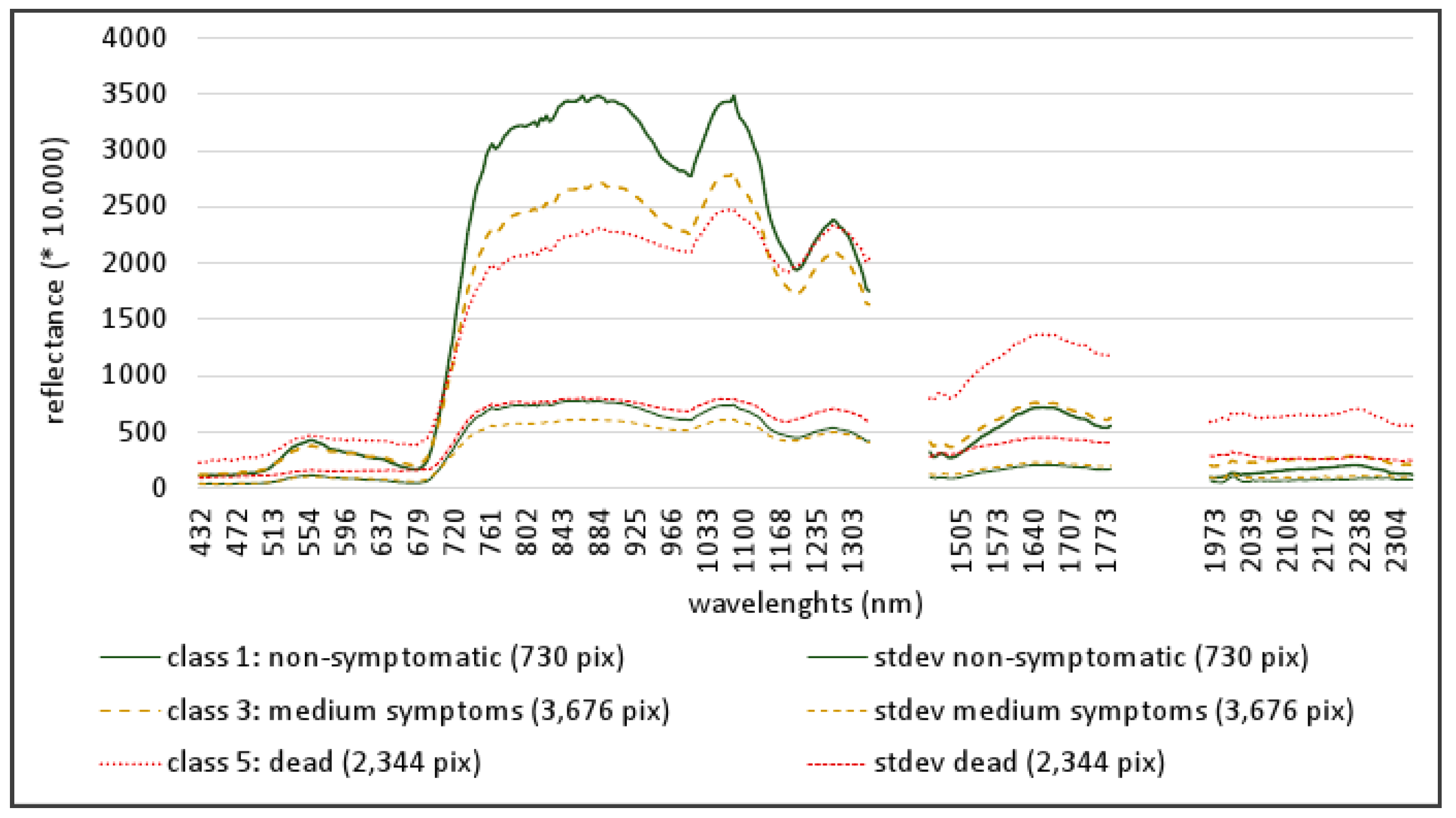
The mean spectra and standard deviations of all reference crowns for three stress levels are illustrated in Figure 7. The spectra of non-symptomatic crowns show the characteristic spectral features for kauri with two even peaks in the NIR2, a steep ascent to the 1074 nm peak and a long steep descent to the pronounced absorption feature at 1215 nm [11]. With increasing stress levels, the chlorophyll absorption in the visible spectral range decreases, especially in the blue and red regions, which leads to a decline in the “green peak” from 409 to 360 reflectance between the non-symptomatic and medium-stress stages. Lower overall reflectance in the NIR1 and a reduced absorption in the red lead to a blue shift in the red-edge spectral region at around 750 nm. The NIR plateau at 880 nm, the reflectance “peak” at 1070 nm and the following water absorption feature decline significantly, which leads to a flattening of the adjacent slopes, so that the spectra lose their characteristic “kauri signature”. The mean reflectance at the NIR1 plateau around 880 nm drops between the non-symptomatic and medium stress levels from 3470 to 2695. However, the decline in the reflectance feature at 1280 nm is less distinct with a drop of reflectance values from 2323 to 2067. Also noticeable is a blue shift in the water vapour valley at 1150 to 1190 nm. Stress responses in the SWIR region include a rise in overall reflectance values, a steeper slope in the SWIR1 region and more distinct absorption features. The difference in SWIR1 values is most distinct between the mean spectra from medium stress levels and dead crowns with a raise at 1650 nm from 760 to 1360 reflectance. In addition, the standard deviation increases with increasing stress levels and is particularly high for the mean spectra of dead trees in the SWIR region.

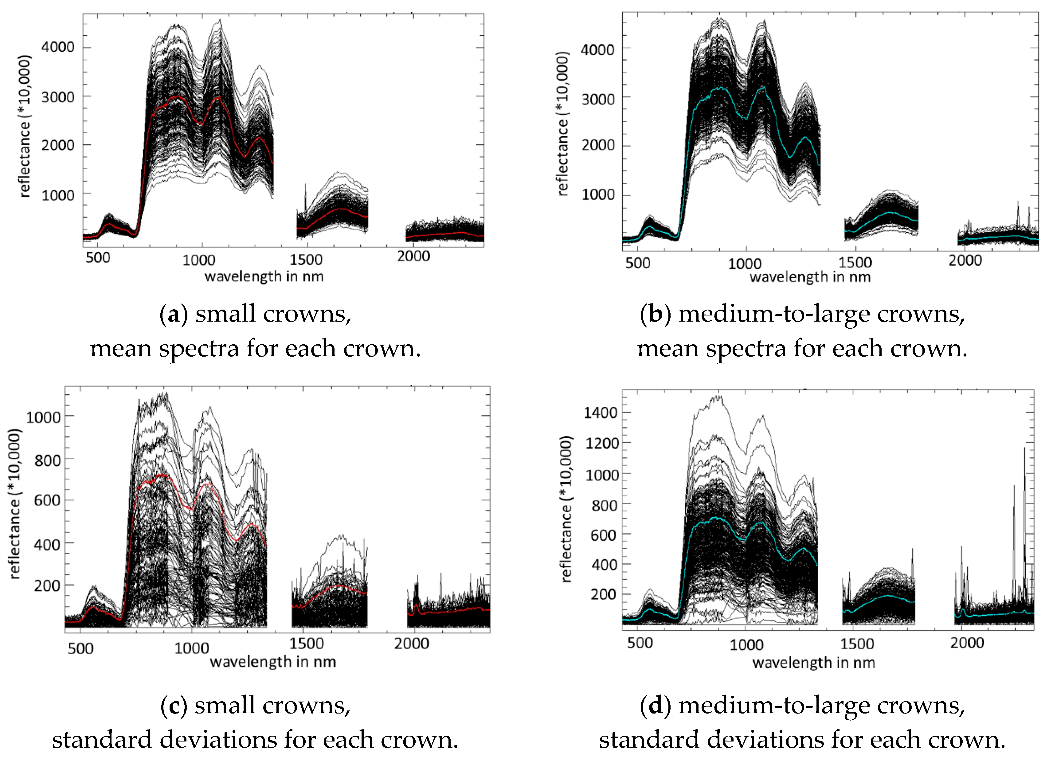
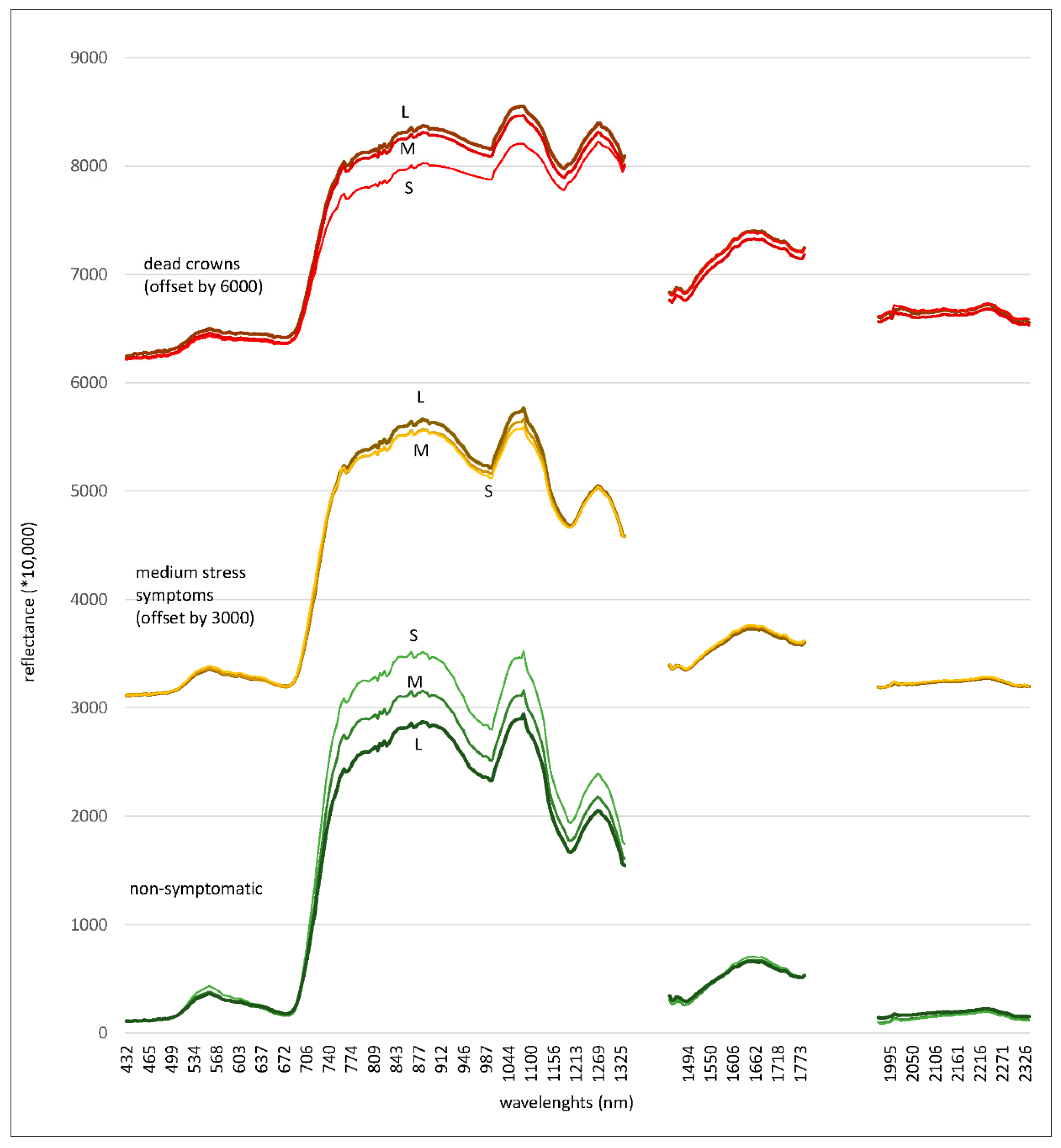
While the overall spectral patterns of the different crown sizes (Figure 8) are similar to the mean spectra of all size classes combined (Figure 7), there are some distinct differences between the size classes. In the non-symptomatic condition, the smaller crown sizes show higher reflectance values, with more pronounced reflectance “peaks”, especially in the green and SWIR1 spectral region, than the medium and large crown sizes. With increasing stress symptoms, the reflectance values of smaller crowns decline at a higher rate than the reflectance values of larger crowns. The spectra of non-symptomatic large crowns show a slightly lower absorption in the blue and red bands and overall lower reflectance in the green and NIR spectral range.

3.3. Objective 1: Best Correlating Band and Index Combinations with Canopy Stress Symptoms

Table 3. Indices and regression results for the full spectral range (VIS to SWIR2). Resulting correlations (corr), mean absolute errors (MAE) and root mean squared errors (RMSE) are given for a Random Forest (RF), M5P and Linear Regression (LR) on selected index combinations in the VIS-SWIR2 spectral range. The analysis was carried out in WEKA on 1258 reference crowns on symptom classes in the range from 1 to 5 with a random 3-fold split in 1000 repetitions. Bold text marks the four most important wavelengths in the respective index combination.

Crown /	# of	Centre Wavelengths of Selected Bands in nm 2					Indices	RF			M5P			LR
Stand Sizes	Bands	VIS	NIR1	NIR2	SWIR1	SWIR2		corr 4 (stdev)	MAE 3	RMSE	corr 4 (stdev)	MAE 3	RMSE	corr 4 (stdev)	MAE 3	RMSE
Best Index Combinations for All Crown Sizes
All Crown Sizes	10	450, 550, 670	800	1094, 1205	1510, 1680	2090, 2210	NDVI-H, LWVI2, mSWIRVI, NDNI, BGI, SR(670,800)	0.938 (0.01)	0.25	0.4	0.93 (0.01)	0.28	0.43	0.91 (0.01)	0.36	0.49
	6 1	450, 550, 670	800	1094, 1205			NDVI-H, LWVI2, BGI, SR(670,800)	0.932 (0.01)	0.27	0.42	0.93 (0.01)	0.28	0.43	0.90 (0.01)	0.37	0.5
	4	670	800	1094, 1205			NDVIHa, LWVI2, SR(670,800)	0.926 (0.01)	0.28	0.44	0.93 (0.01)	0.28	0.44	0.90 (0.01)	0.38	0.51
Baseline Index Combination (6 Bands, 4 Indices) Applied to Different Crown Sizes in Individual Models
Small	6	450, 550, 670	800	1094, 1205			NDVI-H, LWVI2, BGI, SR(670,800)	0.919 (0.02)	0.39	0.55	0.91 (0.02)	0.43	0.58	0.90 (0.01)	0.47	0.6
Medium	6	450, 550, 670	800	1094, 1205			NDVI-H, LWVI2, BGI, SR(670,800)	0.945 (0.01)	0.25	0.38	0.93 (0.01)	0.3	0.42	0.91 (0.01)	0.36	0.48
Large	6	450, 550, 670	800	1094, 1205			NDVI-H, LWVI2, BGI, SR(670,800)	0.887 (0.05)	0.18	0.34	0.86 (0.05)	0.26	0.39	0.86 (0.05)	0.26	0.39
4-Band Index Combination Applied to Different Crown Sizes in Individual Models
Small	6	670	800	1094, 1205			NDVI-H, LWVI2, SR(670,800)	0.915 (0.02)	0.39	0.56	0.91 (0.02)	0.43	0.58	0.90 (0.01)	0.47	0.6
Medium	6	670	800	1094, 1205			NDVI-H, LWVI2, SR(670,800)	0.936 (0.01)	0.26	0.41	0.93 (0.01)	0.3	0.43	0.91 (0.01)	0.36	0.49
Large	6	670	800	1094, 1205			NDVI-H, LWVI2, SR(670,800)	0.878 (0.05)	0.18	0.35	0.86 (0.05)	0.26	0.39	0.86 (0.05)	0.26	0.39
Baseline Index Combination (6 Bands, 4 Indices) Applied for Crowns in Low and High Forest Stands with Individual Models
Low	6	450, 550, 670	800	1094, 1205			NDVI-H, LWVI2, BGI, SR(670,800)	0.933 (0.01)	0.32	0.49	0.93 (0.01)	0.36	0.51	0.90 (0.01)	0.45	0.58
High	6	450, 550, 670	800	1094, 1205			NDVI-H, LWVI2, BGI, SR(670,800)	0.905 (0.03)	0.2	0.36	0.91 (0.03)	0.23	0.36	0.88 (0.03)	0.29	0.4
Best Index Combinations for Individual Crown Sizes
Small	6	550, 685		1094, 1205	1510, 1680		LWVI2, mRGI, NDNI	0.930 (0.01)	0.36	0.51	0.92 (0.02)	0.4	0.55	0.90 (0.01)	0.46	0.6
Medium	6	670	800		1510, 1680	2090, 2210	NDVI-H, mSWIRVI, NDNI	0.947 (0.01)	0.24	0.37	0.93 (0.01)	0.29	0.42	0.90 (0.01)	0.35	0.5
Large	6	675, 700	819		1600	2090, 2210	MSI, mSRa, mSWIRVI	0.897 (0.05)	0.17	0.32	0.87 (0.04)	0.24	0.37	0.87 (0.04)	0.24	0.37

¹ baseline model with four indices on six wavelengths developed on the mean crown spectra for all crown size classes. ² the bands were resampled to 10 nm bandwidths before calculating the indices. ³ Mean absolute error. ⁴ For a comparison of the performances between the regression models, only the correlation values (corr) should be used, while the MAE and RMSE should only be used to compare the performance of one model for different datasets.

and

Table 4. Indices and regression results for the VIS-NIR1 spectral range. Resulting correlations, mean errors and root mean squared errors (RMSE) are given for a Random Forest (RF), M5P and Linear Regression (LR) on selected index combinations in the VIS-NIR1 spectral range. The analysis was carried out in WEKA on 1258 reference crowns on symptom classes in the range from 1 to 5 with a random 3-fold split in 1000 repetitions. Bold text marks the four most important wavelengths according to the attribute importance for the index selection.

Crown	# of	Centre Wavelengths in nm (10 nm bandwidths)		Indices 1	RF			M5P			LR
Size	Bands	VIS	NIR1		Correlation 4 (Stdev)	MAE 4	RMSE	Correlation 4 (Stdev)	MAE 4	RMSE	Correlation 4 (Stdev)	MAE 4	RMSE
VNIR Index Combinations on All Crown Sizes
All	6 2	550, 685 3, 700, 750	900, 970	mNDVI-A, mRVI, mRGI, GM2, WBI	0.93 (0.01)	0.28	0.43	0.925 (0.01)	0.29	0.44	0.89 (0.01)	0.4	0.53
	5	550, 685 3, 700, 750	900	mNDVI-A, mRGI, mRVI, GM2	0.92 (0.01)	0.29	0.46	0.92 (0.01)	0.31	0.45	0.88 (0.01)	0.4	0.56
VNIR Baseline Index Combination Applied on Individual Crown Sizes with Individual Models
Small	6 2	550, 685 3, 700, 750	900, 970	mNDVI-A, mRVI, mRGI, GM2, WBI	0.90 (0.02)	0.42	0.58	0.90 (0.02)	0.44	0.6	0.89 (0.02)	0.47	0.62
Medium	6 2	550, 685 3, 700, 750	900, 970	mNDVI-A, mRVI, mRGI, GM2, WBI	0.94 (0.01)	0.27	0.38	0.94 (0.01)	0.29	0.4	0.92 (0.01)	0.35	0.45
Large	6 2	550, 685 3, 700, 750	900, 970	mNDVI-A, mRVI, mRGI, GM2, WBI	0.88 (0.04)	0.24	0.34	0.86 (0.04)	0.27	0.38	0.87 (0.04)	0.27	0.37
VNIR Index Combinations in a RF Regression Selected for Different Crown Sizes Separately
Small	5	531, 570, 685	900, 970	mNDVI-A, PRI, WBI	0.90(0.02)	0.43	0.61	0.89(0.02)	0.45	0.63	0.84(0.02)	0.59	0.77
Medium	6	440, 670, 690	800, 900, 970	NDVI-H, WBI, LIC2	0.94(0.01)	0.26	0.39	0.93(0.01)	0.43	0.45	0.89(0.01)	0.38	0.54
Large	5	531, 645	860, 900, 970	mNDVI-A, WBI, MLO	0.89(0.05)	0.18	0.34	0.86(0.05)	0.39	0.39	0.85(0.05)	0.26	0.39
VNIR Baseline Index Combination Applied in Individual Models for Different Stand Situations
Low	6 2	550, 685 3, 700, 750	900, 970	mNDVI-A, mRVI, mRGI, GM2, WBI	0.93 (0.01)	0.34	0.51	0.92 (0.01)	0.37	0.53	0.89 (0.01)	0.47	0.61
High	6 2	550, 685 3, 700, 750	900, 970	mNDVI-A, mRVI, mRGI, GM2, WBI	0.90 (0.03)	0.21	0.37	0.89 (0.03)	0.24	0.38	0.87 (0.02)	0.29	0.42

¹ the order of the indices indicates their importance in the RF regression. ² baseline model for the VNIR1 spectral range with 5 bands on 6 indices. ³ the original wavelengths values for bands on 680 and 690 nm, were replaced with 685 nm, to reduce the number of required bands. ⁴ mean absolute error. ⁴ For a comparison of the performances between the regression models, only the correlation values should be used, while the MAE and RMSE should only be used to compare the performance of one model for different datasets.

give an overview of the regression results for the selected index combinations in the full spectral range and the VNIR1 spectral range. A detailed description of the indices with their attribute importance is provided in

Table A4. RF classification (1000 repetitions, 10-fold cross validation) for the baseline VNIR index combination (6 bands, 5 indices) on 2 aggregated classes, to distinguish dead and dying trees (“class 45”) from the other symptom stages (“class 123”).

	Class 123	Class 45	Total	Users Accuracy
Class 123	1043	13	1056	98.8
Class 45	25	177	202	87.6
Total	1068	190	1258
Producers Accuracy	97.7	93.2		97.0

in Appendix E. Overall, the Random Forest (RF) regression performed best, while the results of the M5P regression were usually better than the linear regression (LR) and equal or slightly lower than the RF regression (Table 3, Figure 9, Tables S1 and S2 in the supplementary material). In the following sections, we use the correlations to the stress symptom classes of the RF regression to compare the results.

3.3.1. Indices for Stress Detection in the Full Spectral Range (VIS–SWIR2)

The best band combination (“baseline combination”) for a six-band sensor on the full spectral range achieved a correlation of 0.932 in a RF regression (Table 3). It includes four indices with a Normalized Vegetation Index from Haboudane (NDVI-H) on NIR1/red bands as the most important index, followed by a simple ratio (SR670, 800) on the same bands, a Leaf Water Vegetation Index 2 (LWVI2) in the NIR2 range and a Blue-Green Pigment Index (BGI). A four-band combination without the blue and green bands was slightly less accurate, with a correlation of 0.926. Additional two indices on four bands in the SWIR1 and SWIR2 regions allow adding the Normalized Difference Nitrogen Index (NDNI) and a modified Shortwave Infrared Green Vegetation Index (mSWIRVI), which enhanced the correlation to 0.94.

An individual RF regression of the six-band combination for the different crown sizes resulted in a lower performance of only the small (0.92) and large (0.89) crowns than the results for all crown sizes (0.93), while the results for the medium crowns were unchanged, with 0.93 (Table 3). The same correlations were achieved by directly applying the baseline model that was developed on all crown sizes for the individual size classes. A similar test with the four-band combination without the blue and green bands performed slightly worse than the “baseline” six-band combination. An application of the baseline combination for crowns in different forest stands reached a correlation of 0.94 in low stands and 0.90 for high stands.

With individually selected six-band index combinations for each crown size class, the overall performance could only be slightly enhanced (about 0.01 correlation). The best performing indices for the small crown sizes include the LWVI2 and a modified Red-Green pigment index (mRGI) in combination with an NDNI. The NDVI and mSWIRVI indices were most important for the medium crown sizes, followed by the NDNI. The index combination for large crowns contains the Moisture Stress Index (MSI) with bands in the NIR1 and SWIR1, followed by a simple ratio on red and early red-edge (mSRa) bands and the mSWIRVI with bands in the SWIR2 region.

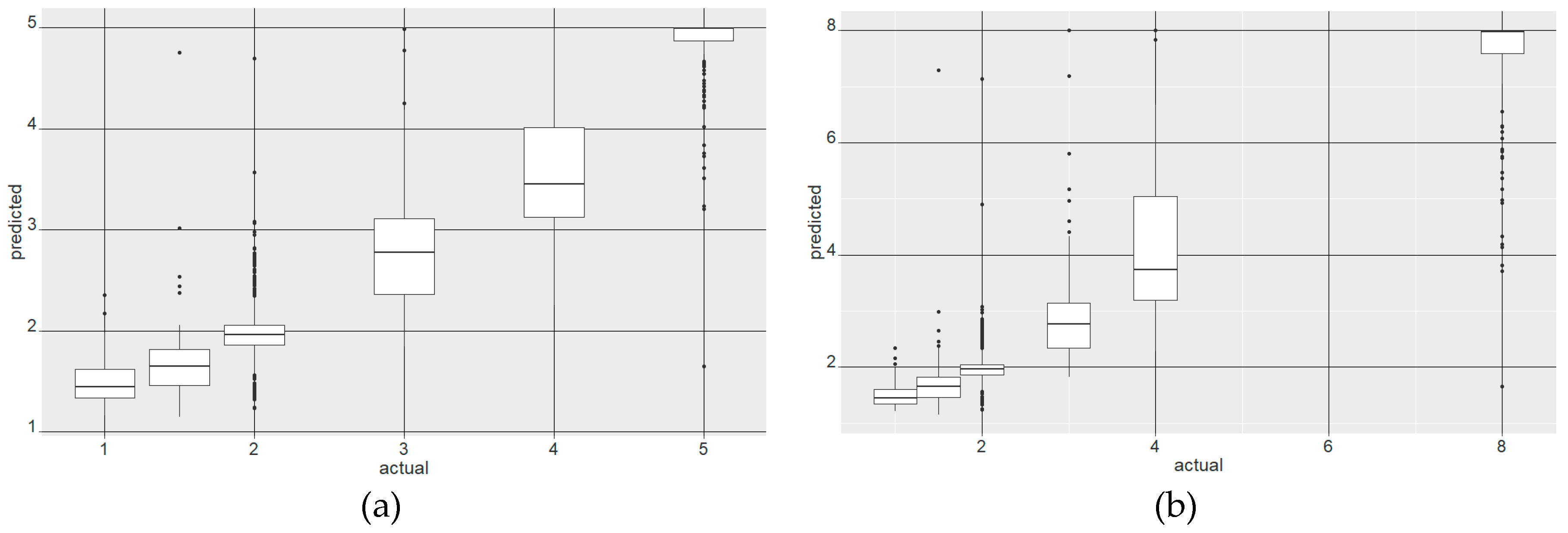
The median values in Figure 9a illustrate a reasonable fit of the baseline model for stress symptoms in all crown sizes. However, the diagram reveals a higher overlap in the first stress categories (1 and 2) as well as the later stages (3 and 4). The later stages of stress and the dead crowns also show a higher range of outliers. A rescaling of the reference values for dead crowns from 5 to 8 (Figure 9b) establishes a more linear relationship between the predicted and actual values. A test of the correlation coefficients after the rescaling revealed that they were mainly unchanged or even partly improved compared to the results of the original scale from 1 to 5 in Table 3.

3.3.2. Indices for Stress Detection in the VIS-NIR1 Spectral Range

Table 4 gives an overview of the performance of selected index combinations in the visible to NIR1 spectral range. A combination of three indices on five wavelengths in the VNIR1 range (437–970 nm) achieved a correlation of 0.92 to the numeric stress symptom classes on all crown sizes. An NDVI on a NIR1 and red band (mNDVI-A 900 and 685 nm) had the highest attribute importance in this combination. Other selected indices include the mRGI, the Gitelson and Merzlyak index-2 (GM2 750 and 700 nm) and a modified Ratio Vegetation Index (mRVI 750 and 685 nm) [108]. The correlation could be increased to 0.93 with an additional band at 970 nm and the Water Band Index (WBI), a ratio on the 900 and 970 nm bands. This index combination is further referred to as the “VNIR1-baseline” index combination. The application of the six-band VNIR1-baseline index combination for crowns in different forest stands results in a correlation of 0.93 for low stands and 0.90 for high stands.

With individual RF models developed for each of the three crown sizes on the VNIR1 baseline combination, the model for medium crown sizes achieved the highest correlation of 0.94, followed by small crowns with 0.90 and large crowns with 0.88 correlation.

Individual attribute selection for the three crown sizes slightly enhances the accuracies. The small crowns achieve a correlation of 0.92 with three indices on bands in the visible (Photochemical Reflectance Index, PRI), red and NIR spectral range (mNDVI-A, WBI). For the medium crowns, three indices with bands in the blue, red and NIR region resulted in a correlation of 0.95. The selection includes the Lichtenthaler Index (LIC2, [109]), which was developed on narrow bands to document a functional decline in chlorophyll fluorescence. Although the 10 nm bandwidths in this setup are probably too coarse for this purpose, the LIC2 band combination performed better than a modified Blue-Red Pigment Index (BRI) [110] on the 450 to 685 nm bands.

The index selection for the large crown sizes has the lowest correlation, with 0.89, and includes an NDVI on a red and NIR1 band, the WBI on the 900 and 970 nm bands and a blue-red ratio (M. Locherer Chlorophyll Index (MLO 531/645) [111]).

3.4. Objective 2: Test Performance of Pre-Selected Index Combinations

The selected band combination for the identification of kauri includes five indices on three wavelengths in the red to NIR1 region (670, 700 and 800 nm) and two wavelengths in the NIR2 region (1074 and 1209 nm) [11] (

Table 5. Index selection for the identification of kauri defined by Meiforth et al. (2019) [11].

Name	Equation	Name, Description	Literature
SR800	$=\frac{R800}{R670}$	Simple Ratio 800/670 chlorophyll concentration and LAI	[108]
SR708	$=\frac{R670}{R708}$	Simple Ratio 670/708 chlorophyll concentration and LAI	[112]
RDVI	$=\frac{R800-R670}{\sqrt{R800+R670}}$	Renormalized Difference VI chlorophyll concentration and LAI	[113]
NDVI	$=\frac{R800-R670}{R800+R670}$	Normalized Difference VI chlorophyll concentration and LAI	[114]
mNDWI-Hyp	$=\frac{log{\left(R1074\right)}^{-1}-log{\left(R1209\right)}^{-1}}{log{\left(R1074\right)}^{-1}+log{\left(R1209\right)}^{-1}}$	Modified Normalized Difference Water Index–Hyperion vegetation canopy water content and canopy structure	[115]

). With an overall correlation of 0.93 in an RF regression for all crown sizes, this index combination performed well in the canopy stress analysis (

Table 6. Resulting correlations, mean absolute errors (MAE) and root mean squared errors (RMSE) for a Random Forest (RF), M5P and Linear Regression (LR) on a 5-band index combination in the VIS-NIR2 range, that was selected for the identification of kauri in Meiforth et al. (2019) [12] (Table 5). The analysis was carried out in WEKA on the mean indices values of 1258 reference crowns with reference symptom classes in the range from 1 to 5 and a random 3-fold split in 1000 repetitions.

Crown/Stand Situation	Random Forest Regression			M5P Regression			Linear Regression
	Corre-Lation 1	MAE	RMSE	Corre-Lation 1	MAE	RMSE	Corre-Lation 1	MAE	RMSE
All Crowns	0.93 (0.01)	0.27	0.43	0.93 (0.01)	0.29	0.44	0.91 (0.01)	0.36	0.49
Small Crowns	0.92 (0.02)	0.39	0.56	0.91 (0.02)	0.42	0.58	0.91 (0.02)	0.46	0.59
Medium Crowns	0.94 (0.01)	0.25	0.39	0.94 (0.01)	0.29	0.42	0.92 (0.01)	0.35	0.46
Large Crowns	0.89 (0.05)	0.19	0.34	0.84 (0.05)	0.27	0.41	0.87 (0.05)	0.25	0.37
Low Stands	0.93 (0.01)	0.33	0.49	0.93 (0.01)	0.35	0.5	0.91 (0.01)	0.43	0.57
High Stands	0.90 (0.03)	0.21	0.36	0.92 (0.01)	0.23	0.36	0.89 (0.01)	0.28	0.38

¹ standard deviations in parentheses.

), with a correlation of 0.93. Further bands in the SWIR that were selected for kauri identification did not improve the accuracy. A test of the five indices for the different crown sizes resulted in the lowest correlation for high crowns (0.89), followed by 0.92 for small crowns and the highest correlation for medium crowns (0.94). The performance for crowns in low stands, with a 0.93 correlation, is higher than for crowns in high forest stands, with 0.90.

3.5. Objective 3: Test Pixel-Based Application

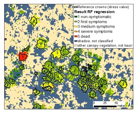
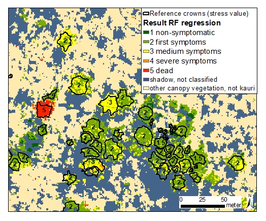
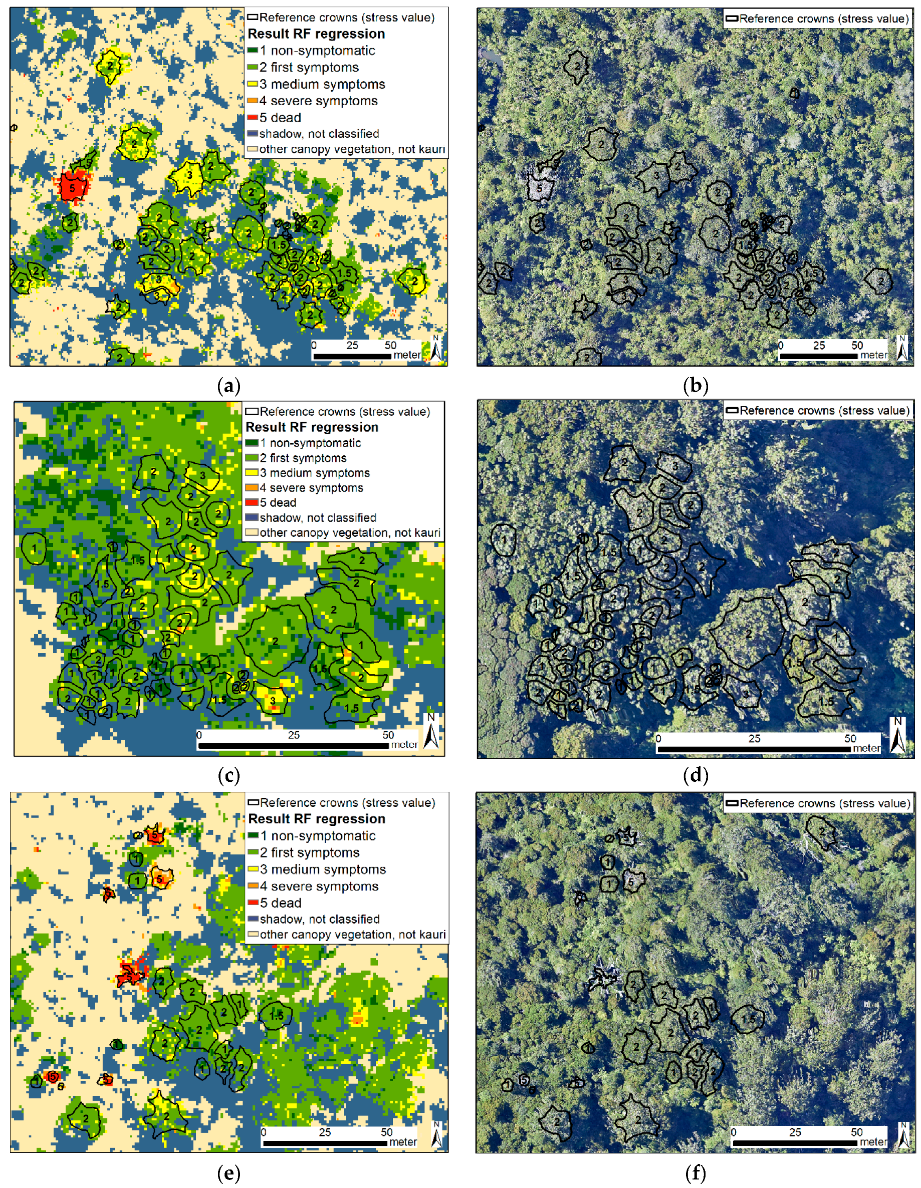
A visual comparison of the pixel-based values in the resulting RF regression map with the crown-based reference values and the aerial images from 2016 and 2017 over the whole area showed an overall good match. Figure 10 shows the resulting map and the aerial image from 2016 three scenes which cover both open and closed stands with larger and smaller tree sizes in all symptom stages. The manual comparison showed that dead and dying trees are classified well, and the heterogeneous stress patterns in larger and partly dying crowns were also described correctly.

4. Discussion

4.1. Discussion: Crown Variability and Crown Spectra in Different Stress Levels

The higher variability of reflectance values between different kauri crowns compared to the within-crown variability (Figure 6) indicates that sites effects or other environmental factors account for the spectra response of the trees at the crown level. The higher spectral variability between the different crowns in the small size group is most likely caused by mixed pixels with neighbouring areas. In a non-symptomatic stage, the overall high spectral variability in the NIR region reflects the importance and range of structural characteristics for the spectra of kauri crowns like the crown architecture, canopy thickness, leaf area and leaf angle. The variability in the visible and shortwave infrared bands, in contrast, is comparatively low, which indicates a high absorption by leaf pigments and canopy water (Figure 6 and Figure 7).

In declining kauri canopies, the loss of photosynthetic foliage causes reduced chlorophyll and water absorption, which leads to a characteristic increase in reflectance values in the VIS and SWIR spectral regions (Figure 7). The overall lower reflectance and less pronounced water absorption features in the NIR range in declining crowns can be explained by reduced scattering processes and water concentration due to foliage loss. Strong water absorption features from green leaf material dominate the spectral response in the SWIR region at high LAI [69], the loss of leaf material and canopy water and a relative increase in woody stem material and litter allows the spectral absorption features of cellulose and lignin in the SWIR regions to emerge at around 1754, 2100 and 2262 nm [116,117]. The slightly steeper slope in the SWIR1 region from 1500 to 1680 nm in declining trees indicates a decrease in chlorophyll-bound nitrogen with a distinct absorption around 1510 nm [69]. The higher percentage of stem material in declining canopies contributes to a higher reflectance in the red spectral region, a decreased magnitude of the NIR plateau, an increase in SWIR reflectance and an equalization of the local maxima in the NIR and SWIR regions [118].

The increasing spectral variability with rising stress levels, especially in dead crowns, can be explained by the spectral influence of understorey vegetation, ground material and a variable number of epiphytes, climbers and dry litter in the crowns. The remaining vegetation and water absorption features in the mean spectra of dead crowns are caused by photosynthetic active sub-canopy vegetation and epiphytes. These effects correspond to the observations of Baret et al. (1995) [119] and Asner (2008) [118] that the crown reflectance is mainly influenced by the gap fraction when the vegetation cover is less than 70%–80%.

The phenological differences between the dense homogenous foliage in smaller kauri compared to the open, heterogeneous crown structure of large kauri is also reflected in their spectral response. Already in the non-symptomatic stage, large kauri crowns show a higher within-crown spectral variability, which is caused by the stronger influence of internal shadows, woody material and understory reflectance in the open dome shape crown structure. The higher reflectance of small non-symptomatic kauri crowns compared to larger crown sizes corresponds to the findings of Rautiainen (2018) [70]. She observed a higher reflectance for an immature Norway spruce stand compared to a mature stand at all spatial scales, which she attributed to different leaf biochemical properties, denser foliage and a higher tree density in smaller stands, with less shadowing between the crowns. With increasing stress levels, the NIR reflectance values of the smaller crown sizes decline disproportionately faster than the NIR response of larger crown sizes (Figure 8). This effect can be explained by the stronger influence of photosynthetic active green undergrowth and epiphytes in the more open larger crown sizes.

4.2. Discussion Objective 1: Index Combinations for Stress Detection

A description of the observed spectral responses in kauri crowns in different stress and growth stages requires the combination of indices in different spectral ranges. With overall high correlations of 0.93 in a RF regression for five canopy stress symptom classes, the six-band baseline combinations in both the full spectral range and the VNIR1 range (Table 4) are well suited to describe stress symptoms in kauri canopies of all sizes. The continuous output range of the chosen regression approach allows a detailed assessment of the severity of stress symptoms, especially in the early symptom stages. The most important VIs for stress detection for all crown and stand situations are NDVIs and simple ratios with bands in the NIR1 and red spectrum, which describe the efficiency drop of photosynthetic absorption in the red band and the decrease of reflectance in the NIR1 region. The 900 nm NIR band of the mNDVI-A [120] that was selected in the VNIR1 range is also sensitive to the amount of dry matter, which might compensate for the missing SWIR bands in the VNIR1 selection. In the more advanced stages, the loss of foliage and branch material causes structural changes and a further loss of canopy water, which are captured in the selected Leaf Water Vegetation Index (LWVI), with bands in the NIR2 spectral region (1094, 1205 nm) [121] and the WBI and MSI for the VNIR1 spectral range.

To account for the spectral properties in different size classes, we tested two stratified approaches: A distinction between small, medium and large crown sizes according to their mean diameter and separation of crowns in low and high forest stands. In small kauri crowns sizes with denser foliage, indices in the visible spectrum like the mRGI, BGI2 [110,122] and PRI were selected. These are more sensitive to pigment changes, and they perform better than NIR1/red band combinations in dense foliage with high LAI and high concentrations of chlorophyll when NIR1/red indices easily saturate [122]. Furthermore, the NDNI (1510 and 1680 nm) that was selected for small crown sizes in the full spectral range is sensitive to changes in foliar nitrogen content [69,123]. The mRGI is also included in the VNIR1 baseline combination together with the GM2 index that captures a blue shift of the red edge region [124]. For the more open medium and large crown sizes, the selected mSWIRVI with bands in the SWIR2 region (2090 and 2210 nm) on the full spectral range is sensitive to the influence of dry matter with cellulose reflectance [117,125].

While these individual band and index selections for different crown sizes showed the highest performances for both the full spectral range and the VNIR range, individual models for the different crown sizes on the same 6-band baseline combination performed nearly as well. The slightly lower correlations on the baseline combination for large crowns (0.89 and 0.88) compared to medium (0.94 and 0.94) and small crowns sizes (0.92 and 0.90) can most likely be explained by the higher spectral variability in the larger crowns already in the non-symptomatic stages. Moreover, some large crowns show heterogeneous stress patterns with different symptom stages in different parts of the crown. Medium crown sizes are less influenced by mixed pixels than small crowns and more homogenous than larger crowns. Moreover, the larger number of medium crowns in the reference crown set, according to the crown size distribution in the study areas, might contribute to the better fit of the model for medium crown sizes.

Compared to the application of the baseline indices to small and large crowns, the correlations of different RF models for crowns in low and high forest stands on the same index combination are slightly higher, with 0.94 (VNIR1: 0.93) for low stands and 0.90 (VNIR1 0.90) for high forest stands. These higher accuracies can presumably be attributed to the influence of the easier to describe medium crown sizes in both stand situations (Figure 5).

4.3. Discussion Objective 2: Performance of Band Selection for Kauri Detection

The five-band index combination that was selected to identify kauri trees in Meiforth et al. (2019) [12] with bands in the red, red-edge, NIR1 and NIR2, is similar to the baseline combination for stress detection on the full spectral range. It showed a comparably high correlation of 0.92 with the stress symptom classes on all crown sizes. The lower performance of this index combination for small crowns with denser foliage can be explained by the lack of bands in the blue and green spectrum, which are sensitive to pigment-related reflectance features. The index combination also contains the mNDWI-H, which describes the characteristic spectral reflectance and absorption features of kauri in the NIR2 (1074, 1209). These spectral features are most likely caused by photon scattering in the thick kauri leaves at the mesophyll and the air–cell–wall interfaces, the characteristic spiky foliage surface and the open crown structure in larger kauri that allow the woody material from the massive stem and branches to influence the crown reflectance. The more a kauri crown declines and loses its foliage, the more it also loses these characteristic structural features. In conclusion, this five-band index combination can be used for stress detection in kauri crowns. However, it should be improved for smaller crowns by adding a green band.

4.4. Discussion Objective 3: Pixel-Based Application

The observed high correlation of the pixel-based implementation with the visible stress symptoms in a manual comparison with the aerial images (Figure 10) indicates that this is a practical approach. However, the results should be tested more thoroughly, ideally with quantitative sub-canopy reference data, that need to be accurately aligned with the remote sensing image used in the analysis. The aerial image from 2017 that matches the same season as the hyperspectral data was unfortunately not sufficiently aligned for such an analysis. A pixel-based approach allows for an easy application since this method does not require a prior crown segmentation. It enables a more detailed assessment of larger crowns, which often show heterogenic symptom patterns. It also gives more flexibility to define the aggregated reporting units from single crowns to homogenous forest stands. Furthermore, it allows the direct usage of the pixel-based kauri mask, described in Meiforth et al. (2019) [12]. The crown-based results indicate that further improvements of the pixel-based regression map can be achieved in separate analyses for low and high forest stands. For the large-area monitoring of forest situations like the Waitakere Ranges with a multispectral sensor, we recommend a pixel size at around 0.5 m, which is large enough to level out extremes but small enough to capture small crown sizes.

4.5. Discussion: Application and Further Analysis

While the RF regression results in high correlations between the predicted and actual values, a slightly non-linear relationship, especially towards the dead and dying crowns, results in a shift between the predicted and actual value range. A rescaling of the value for the dead trees from value 5 to value 8, improves the match between the predicted and actual values (Figure 9). The resulting levels “5 to 8” describe different portions of dead branch material and shadows, which cause the extreme values. The correlation coefficients for the rescaled value range remained mainly unchanged and even partly improved compared to the original range from 1 to 5. The rescaling simplifies the interpretation of the predicted values, while the new resulting values from 6 to 8 have no influence on the practical implementation since all crowns with values equal or higher 5 can be treated as “dead”.

Another possibility to address the non-linearity in the higher levels of stress symptoms, is to first distinguish the dead and dying trees in a binary classification and then apply the regression to the remaining first to medium symptom stages, which feature a more linear relationship. A test with a binary RF classification showed that the aggregated class “dead/dying” can be distinguished with a high overall accuracy of 97% and users and producers accuracies of 87.6% respective 93.32% (Table A4 in Appendix E). This approach should be tested in further studies.

The use of the resulting maps for management purposes requires an interpretation to translate the detected stress symptoms into a health assessment since the canopy stress symptoms in kauri can have a range of causes besides a PA infection, such as water shortage and unfavourable growing conditions [4,126]. The application of time series allows detecting characteristic temporal trends and spatial patterns of infection symptoms and can help to distinguish between different causes of stress [15,127,128,129,130].

High spectral resolution satellite data like Sentinel-2 and WorldView02 should be tested for cost-efficient large-area stress detection in time series. The combination with LiDAR attributes can also improve stress detection, especially for more advanced stress levels with textural and structural changes in the canopy caused by defoliation [131,132,133,134]. The challenging sub-pixel co-location between optical and LiDAR datasets might be overcome with new multispectral waveform LiDAR sensors that allow the direct combination of LiDAR data with multispectral wavelengths in one dataset [135].

5. Conclusions

The analysis of an airborne AISA hyperspectral image proved that a combination of six spectral bands in the VNIR1 range (550–970 nm) is sufficient to capture the full range of canopy stress symptoms in kauri trees on a numeric scale from 1 to 5 with a high correlation of 0.93 (mean error of 0.27, RMSE 0.43) in a Random Forest (RF) regression. To establish a more linear relationship between predicted and actual values, we recommend a rescaling the value for dead trees from 5 to 8. The easier to implement M5P algorithm performed nearly as well as a more complicated RF regression model. The most important indices are sensitive to structural changes and canopy water, while stress symptoms in smaller kauri crowns with denser foliage are best described with additional bands in the green and blue spectrum, which are sensitive to pigment changes.

The study was designed to be applicable to large-area monitoring with a large representative reference set of 1258 crowns, and selected bandwidths of 10 nm that can be used on multispectral sensors. Based on the reference crowns and field assessment data, we developed a numeric assessment scheme for canopy stress symptoms in kauri trees on RGB aerial images, which are better suited for an assessment of the upper crown canopy than a limited view through the undergrowth and canopy from the ground.

Comparable correlations to the VNIR1 selection were achieved with six bands in the VNIR2 spectrum (450–1205 nm), while additional bands in the SWIR enhanced the correlation only slightly, to 0.94. However, we recommend the use of the six-band combination in the VNIR1 range instead of the full spectral range since it is easier to implement, the VNIR bands have a higher signal to noise ratio and are less influenced by species-specific structural crown attributes.

The spectral differences of kauri crowns in different size classes respective stand situations advise a stratified approach. We recommend the application of the six-band baseline combination with individual models for pre-selected crown sizes, respective crowns in low and high forest stands.

While the analysis is based on mean crown spectra to match the scale of the reference data, an easier to apply pixel-based application seem to match well with the observed stress symptoms in the field and aerial images. However, this approach needs to be tested more thoroughly in other areas with matching reference data.

The results of this study have important implications for the monitoring of canopy stress symptoms in kauri trees in New Zealand. The objective, cost-efficient method for large-area monitoring of canopy stress symptoms with a multispectral sensor will help to target the required fieldwork and support management decisions to prevent the further spread of the kauri dieback disease.

References

- Wyse, S.V.; Burns, B.R.; Wright, S.D. Distinctive vegetation communities are associated with the long-lived conifer Agathis australis (New Zealand kauri, Araucariaceae) in New Zealand rainforests. Austral Ecol. 2014, 39, 388–400. [Google Scholar] [CrossRef]
- Shortland, T.; Wood, W. Kia Toitu He Kauri, Kauri Dieback Tangata Whenua Roopu Cultural Impact Assessment; Repo Consultancy Limited: Whangarei, New Zealand, 2011. [Google Scholar]
- Beever, R.E.; Waipara, N.W.; Ramsfield, T.D.; Dick, M.A.; Horner, I.J. Kauri (Agathis australis) under threat from Phytophthora. Phytophthoras For. Nat. Ecosyst. 2009, 74. [Google Scholar]
- Sanson, J. Independent Review of the State of Kauri Dieback Knowledge; Lincoln University: Lincoln, New Zealand, 2016. [Google Scholar]
- MPI. kauri Dieback Distribution. A Map Published on the Kauri Dieback Website. Ministry for Primary Industries, Biosecurity New Zealand, Wellington. 2020. Available online: https://www.kauridieback.co.nz/media/2037/kauri-dieback-distribution_20190930_350dpi.jpg (accessed on 1 February 2020).
- Alastair Jamieson, L.H.; Nick, W.; Jack, C. Survey of Kauri Dieback in the Hunua Ranges; Pseudomonas & Phytophthora; New Zealand Plant Protection Society: Auckland, New Zealand, 2011; pp. 60–65. [Google Scholar]
- Waipara, N.; Hill, S.; Hill, L.; Hough, E.; Horner, I. Surveillance methods to determine tree health, distribution of kauri dieback disease and associated pathogens. N. Z. Plant Prot. 2013, 66, 235–241. [Google Scholar] [CrossRef] [Green Version]
- MPI. Kia toitu he kauri–Keep kauri standing. New Zealands strategy for managing kauri dieback disease. Minist. Prim. Ind. 2014, 2014, 24. [Google Scholar]
- Ecroyd, C. Biological flora of New Zealand 8. Agathis australis (D. Don) Lindl.(Araucariaceae) Kauri. N. Z. J. Bot. 1982, 20, 17–36. [Google Scholar] [CrossRef]
- Steward, G.A.; Beveridge, A.E. A review of New Zealand kauri (Agathis australis (D. Don) Lindl.): Its ecology, history, growth and potential for management for timber. N. Z. J. For. Sci. 2010, 40, 33–59. [Google Scholar]
- Meiforth, J.J.; Buddenbaum, H.; Hill, J.; Shepherd, J.; Norton, D.A. Detection of New Zealand Kauri Trees with AISA Aerial Hyperspectral Data for Use in Multispectral Monitoring. Remote Sens. 2019, 11, 2865. [Google Scholar] [CrossRef] [Green Version]
- Meiforth, J.J. Photos, Waitakere Ranges Photo Staken During Fieldwork in January to March 2016; Waitakere Ranges: Auckland, New Zealand, 2016. [Google Scholar]
- Auckland Council. Helicopter Survey for Kauri Dieback in the Waitakere Ranges; Unpublished aerial photos; Auckland Council: Auckland, New Zealand, 2016. [Google Scholar]
- Scott, P.; Williams, N. Phytophthora diseases in New Zealand forests. N. Z. J. For. 2014, 59, 14–21. [Google Scholar]
- Hall, R.; Castilla, G.; White, J.; Cooke, B.; Skakun, R.J. Remote sensing of forest pest damage: A review and lessons learned from a Canadian perspective. Can. Entomol. 2016, 148, S296–S356. [Google Scholar] [CrossRef]
- Senf, C.; Seidl, R.; Hostert, P. Remote sensing of forest insect disturbances: Current state and future directions. Int. J. Appl. Earth Obs. Geoinf. 2017, 60, 49–60. [Google Scholar] [CrossRef] [PubMed] [Green Version]
- Stone, C.; Mohammed, C. Application of remote sensing technologies for assessing planted forests damaged by insect pests and fungal pathogens: A review. Curr. For. Rep. 2017, 3, 75–92. [Google Scholar] [CrossRef]
- Wulder, M.A.; Dymond, C.C.; White, J.C.; Leckie, D.G.; Carroll, A.L. Surveying mountain pine beetle damage of forests: A review of remote sensing opportunities. For. Ecol. Manag. 2006, 221, 27–41. [Google Scholar] [CrossRef]
- Silva, C.R.; Olthoff, A.; de la Mata, J.A.D.; Alonso, A.P. Remote monitoring of forest insect defoliation. A review. For. Syst. 2013, 22, 377–391. [Google Scholar]
- Lausch, A.; Erasmi, S.; King, D.; Magdon, P.; Heurich, M. Understanding forest health with remote sensing-part I—A review of spectral traits, processes and remote-sensing characteristics. Remote Sens. 2016, 8, 1029. [Google Scholar] [CrossRef] [Green Version]
- Lausch, A.; Erasmi, S.; King, D.; Magdon, P.; Heurich, M. Understanding forest health with remote sensing-part II—A review of approaches and data models. Remote Sens. 2017, 9, 129. [Google Scholar] [CrossRef] [Green Version]
- Coops, N.; Stanford, M.; Old, K.; Dudzinski, M.; Culvenor, D.; Stone, C. Assessment of Dothistroma needle blight of Pinus radiata using airborne hyperspectral imagery. Phytopathology 2003, 93, 1524–1532. [Google Scholar] [CrossRef] [Green Version]
- Misurec, J.; Kopacková, V.; Lhotakova, Z.; Albrechtova, J.; Hanus, J.; Weyermann, J.; Entcheva-Campbell, P. Utilization of hyperspectral image optical indices to assess the Norway spruce forest health status. J. Appl. Remote Sens. 2012, 6, 063545. [Google Scholar]
- Abdel-Rahman, E.M.; Mutanga, O.; Adam, E.; Ismail, R. Detecting Sirex noctilio grey-attacked and lightning-struck pine trees using airborne hyperspectral data, random forest and support vector machines classifiers. ISPRS J. Photogramm. Remote Sens. 2014, 88, 48–59. [Google Scholar] [CrossRef]
- Fassnacht, F.E.; Latifi, H.; Ghosh, A.; Joshi, P.K.; Koch, B. Assessing the potential of hyperspectral imagery to map bark beetle-induced tree mortality. Remote Sens. Environ. 2014, 140, 533–548. [Google Scholar] [CrossRef]
- Näsi, R.; Honkavaara, E.; Blomqvist, M.; Lyytikäinen-Saarenmaa, P.; Hakala, T.; Viljanen, N.; Kantola, T.; Holopainen, M. Remote sensing of bark beetle damage in urban forests at individual tree level using a novel hyperspectral camera from UAV and aircraft. Urban For. Urban Green. 2018, 30, 72–83. [Google Scholar] [CrossRef]
- Sandino, J.; Pegg, G.; Gonzalez, F.; Smith, G. Aerial mapping of forests affected by pathogens using UAVs, hyperspectral sensors, and artificial intelligence. Sensors 2018, 18, 944. [Google Scholar] [CrossRef] [PubMed] [Green Version]
- Pontius, J.; Martin, M.; Plourde, L.; Hallett, R. Ash decline assessment in emerald ash borer-infested regions: A test of tree-level, hyperspectral technologies. Remote Sens. Environ. 2008, 112, 2665–2676. [Google Scholar] [CrossRef]
- Pu, R.; Kelly, M.; Anderson, G.L.; Gong, P.J.P.E.; Sensing, R. Using CASI hyperspectral imagery to detect mortality and vegetation stress associated with a new hardwood forest disease. Photogramm. Eng. Remote Sens. 2008, 74, 65–75. [Google Scholar] [CrossRef] [Green Version]
- Michez, A.; Piégay, H.; Lisein, J.; Claessens, H.; Lejeune, P. Classification of riparian forest species and health condition using multi-temporal and hyperspatial imagery from unmanned aerial system. Environ. Monit. Assess. 2016, 188, 146. [Google Scholar] [CrossRef] [Green Version]
- Thenkabail, P.S.; Lyon, J.G.; Huete, A. Hyperspectral Remote Sensing of Vegetation; CRC Press: Boca Raton, FL, USA, 2011. [Google Scholar]
- Lawrence, R.; Labus, M. Early detection of Douglas-fir beetle infestation with subcanopy resolution hyperspectral imagery. West. J. Appl. For. 2003, 18, 202–206. [Google Scholar] [CrossRef] [Green Version]
- López-López, M.; Calderón, R.; González-Dugo, V.; Zarco-Tejada, P.; Fereres, E. Early detection and quantification of almond red leaf blotch using high-resolution hyperspectral and thermal imagery. Remote Sens. 2016, 8, 276. [Google Scholar] [CrossRef] [Green Version]
- Lowe, A.; Harrison, N.; French, A.P. Hyperspectral image analysis techniques for the detection and classification of the early onset of plant disease and stress. Plant Methods 2017, 13, 80. [Google Scholar] [CrossRef]
- Dotzler, S.; Hill, J.; Buddenbaum, H.; Stoffels, J. The Potential of EnMAP and Sentinel-2 Data for Detecting Drought Stress Phenomena in Deciduous Forest Communities. Remote Sens. 2015, 7, 14227–14258. [Google Scholar] [CrossRef] [Green Version]
- Garrity, S.R.; Allen, C.D.; Brumby, S.P.; Gangodagamage, C.; McDowell, N.G.; Cai, D.M. Quantifying tree mortality in a mixed species woodland using multitemporal high spatial resolution satellite imagery. Remote Sens. Environ. 2013, 129, 54–65. [Google Scholar] [CrossRef]
- Meng, J.; Li, S.; Wang, W.; Liu, Q.; Xie, S.; Ma, W. Mapping forest health using spectral and textural information extracted from spot-5 satellite images. Remote Sens. 2016, 8, 719. [Google Scholar] [CrossRef] [Green Version]
- Townsend, P.A.; Singh, A.; Foster, J.R.; Rehberg, N.J.; Kingdon, C.C.; Eshleman, K.N.; Seagle, S.W. A general Landsat model to predict canopy defoliation in broadleaf deciduous forests. Remote Sens. Environ. 2012, 119, 255–265. [Google Scholar] [CrossRef]
- Wang, J.; Sammis, T.W.; Gutschick, V.P.; Gebremichael, M.; Dennis, S.O.; Harrison, R.E. Review of satellite remote sensing use in forest health studies. Open Geogr. J. 2010, 3, 28–42. [Google Scholar] [CrossRef]
- Wang, H.; Pu, R.; Zhang, Z. Mapping Robinia Pseudoacacia Forest Health Conditions by Using Combined Spectral, Spatial and Textureal Information Extracted from Ikonos Imagery. Int. Arch. Photogramm. Remote Sens. Spatial Inf. Sci. 2016, XLI-B8, 1425–1429. [Google Scholar] [CrossRef] [Green Version]
- Waser, L.T.; Küchler, M.; Jütte, K.; Stampfer, T. Evaluating the potential of WorldView-2 data to classify tree species and different levels of ash mortality. Remote Sens. 2014, 6, 4515–4545. [Google Scholar] [CrossRef] [Green Version]
- White, J.C.; Wulder, M.A.; Brooks, D.; Reich, R.; Wheate, R.D. Detection of red attack stage mountain pine beetle infestation with high spatial resolution satellite imagery. Remote Sens. Environ. 2005, 96, 340–351. [Google Scholar] [CrossRef]
- Aasen, H.; Honkavaara, E.; Lucieer, A.; Zarco-Tejada, P.J. Quantitative remote sensing at ultra-high resolution with UAV spectroscopy: A review of sensor technology, measurement procedures, and data correction workflows. Remote Sens. 2018, 10, 1091. [Google Scholar] [CrossRef] [Green Version]
- Coops, N.C.; Goodwin, N.; Stone, C.; Sims, N. Application of narrow-band digital camera imagery to plantation canopy condition assessment. Can. J. Remote Sens. 2006, 32, 19–32. [Google Scholar] [CrossRef]
- Pietrzykowski, E.; Sims, N.; Stone, C.; Pinkard, L.; Mohammed, C. Predicting Mycosphaerella leaf disease severity in a Eucalyptus globulus plantation using digital multi-spectral imagery. South. Hemisph. For. J. 2007, 69, 175–182. [Google Scholar] [CrossRef]
- Zarco-Tejada, P.J.; Berni, J.A.; Suárez, L.; Sepulcre-Cantó, G.; Morales, F.; Miller, J.R. Imaging chlorophyll fluorescence with an airborne narrow-band multispectral camera for vegetation stress detection. Remote Sens. Environ. 2009, 113, 1262–1275. [Google Scholar] [CrossRef]
- Meddens, A.J.; Hicke, J.A.; Vierling, L.A. Evaluating the potential of multispectral imagery to map multiple stages of tree mortality. Remote Sens. Environ. 2011, 115, 1632–1642. [Google Scholar] [CrossRef]
- Asner, G.P. Hyperspectral remote sensing of canopy chemistry, physiology, and biodiversity in tropical rainforests. In Hyperspectral Remote Sensing of Tropical and Sub-Tropical Forests; Kalacsca, M., Sances, G.A., Eds.; Azofeita CRC Press: Boca Raton, FL, USA, 2008; pp. 261–296. [Google Scholar]
- Jensen, J.R. Introductory Digital Image Processing: A Remote Sensing Perspective, 4th ed.; Pearson Education, Inc.: Glenview, IL, USA, 2016. [Google Scholar]
- Kaufmann, H.E.A. Hyperspectral Algorithms: Report in the Frame of EnMAP Preparation Activities; Deutsches GeoForschungsZentrum GFZ: Potsdam, Germany, 2010. [Google Scholar]
- Berni, J.; Zarco-Tejada, P.; Sepulcre-Cantó, G.; Fereres, E.; Villalobos, F. Mapping canopy conductance and CWSI in olive orchards using high resolution thermal remote sensing imagery. Remote Sens. Environ. 2009, 113, 2380–2388. [Google Scholar] [CrossRef]
- Calderón, R.; Navas-Cortés, J.; Zarco-Tejada, P. Early detection and quantification of Verticillium wilt in olive using hyperspectral and thermal imagery over large areas. Remote Sensing. 2015, 7, 5584–5610. [Google Scholar] [CrossRef] [Green Version]
- Strasser, R.J.; Srivastava, A. Polyphasic chlorophyll a fluorescence transient in plants and cyanobacteria. Photochem. Photobiol. 1995, 61, 32–42. [Google Scholar] [CrossRef]
- Zarco-Tejada, P.J.; Miller, J.R.; Mohammed, G.; Noland, T.L.; Sampson, P. Vegetation stress detection through chlorophyll a+ b estimation and fluorescence effects on hyperspectral imagery. J. Environ. Qual. 2002, 31, 1433–1441. [Google Scholar] [CrossRef] [PubMed]
- Blackburn, G.A. Hyperspectral remote sensing of plant pigments. J. Exp. Bot. 2006, 58, 855–867. [Google Scholar] [CrossRef] [Green Version]
- Suárez, L.; Zarco-Tejada, P.J.; Sepulcre-Cantó, G.; Pérez-Priego, O.; Miller, J.; Jiménez-Muñoz, J.; Sobrino, J. Assessing canopy PRI for water stress detection with diurnal airborne imagery. Remote Sens. Environ. 2008, 112, 560–575. [Google Scholar] [CrossRef]
- Hunt Jr, E.R.; Rock, B.N. Detection of changes in leaf water content using near-and middle-infrared reflectances. Remote Sens. Environ. 1989, 30, 43–54. [Google Scholar] [CrossRef]
- Gao, B.-C. NDWI—A normalized difference water index for remote sensing of vegetation liquid water from space. Remote Sens. Environ. 1996, 58, 257–266. [Google Scholar] [CrossRef]
- Peñuelas, J.; Filella, I.; Biel, C.; Serrano, L.; Save, R. The reflectance at the 950–970 nm region as an indicator of plant water status. Int. J. Remote Sens. 1993, 14, 1887–1905. [Google Scholar] [CrossRef]
- Hendry, G.A.; Houghton, J.D.; Brown, S.B. The degradation of chlorophyll-a biological enigma. New Phytol. 1987, 1987, 255–302. [Google Scholar] [CrossRef]
- Gitelson, A.A.; Gritz, Y.; Merzlyak, M.N. Relationships between leaf chlorophyll content and spectral reflectance and algorithms for non-destructive chlorophyll assessment in higher plant leaves. J. Plant Physiol. 2003, 160, 271–282. [Google Scholar] [CrossRef] [PubMed]
- Woolley, J.T. Reflectance and transmittance of light by leaves. Plant Physiol. 1971, 47, 656–662. [Google Scholar] [CrossRef] [PubMed] [Green Version]
- Tucker, C.J. Red and photographic infrared linear combinations for monitoring vegetation. Remote Sens. Environ. 1979, 8, 127–150. [Google Scholar] [CrossRef] [Green Version]
- Glenn, E.; Huete, A.; Nagler, P.; Nelson, S. Relationship between remotely-sensed vegetation indices, canopy attributes and plant physiological processes: What vegetation indices can and cannot tell us about the landscape. Sensors 2008, 8, 2136–2160. [Google Scholar] [CrossRef] [Green Version]
- Jago, R.A.; Cutler, M.E.; Curran, P.J. Estimating canopy chlorophyll concentration from field and airborne spectra. Remote Sens. Environ. 1999, 68, 217–224. [Google Scholar] [CrossRef]
- Eitel, J.U.; Vierling, L.A.; Litvak, M.E.; Long, D.S.; Schulthess, U.; Ager, A.A.; Krofcheck, D.J.; Stoscheck, L. Broadband, red-edge information from satellites improves early stress detection in a New Mexico conifer woodland. Remote Sens. Environ. 2011, 115, 3640–3646. [Google Scholar] [CrossRef]
- Kim, Y.; Glenn, D.M.; Park, J.; Ngugi, H.K.; Lehman, B.L. Hyperspectral image analysis for water stress detection of apple trees. Comput. Electron. Agric. 2011, 77, 155–160. [Google Scholar] [CrossRef]
- Penuelas, J.; Baret, F.; Filella, I. Semi-empirical indices to assess carotenoids/chlorophyll a ratio from leaf spectral reflectance. Photosynthetica 1995, 31, 221–230. [Google Scholar]
- Serrano, L.; Penuelas, J.; Ustin, S.L. Remote sensing of nitrogen and lignin in Mediterranean vegetation from AVIRIS data: Decomposing biochemical from structural signals. Remote Sens. Environ. 2002, 81, 355–364. [Google Scholar] [CrossRef]
- Rautiainen, M.; Lukeš, P.; Homolova, L.; Hovi, A.; Pisek, J.; Mottus, M. Spectral properties of coniferous forests: A review of in situ and laboratory measurements. Remote Sens. 2018, 10, 207. [Google Scholar] [CrossRef] [Green Version]
- Zagolski, F.; Pinel, V.; Romier, J.; Alcayde, D.; Fontanari, J.; Gastellu-Etchegorry, J.; Giordano, G.; Marty, G.; Mougin, E.; Joffre, R. Forest canopy chemistry with high spectral resolution remote sensing. Int. J. Remote Sens. 1996, 17, 1107–1128. [Google Scholar] [CrossRef]
- Gong, P.; Pu, R.; Biging, G.S.; Larrieu, M.R. Estimation of forest leaf area index using vegetation indices derived from Hyperion hyperspectral data. IEEE Trans. Geosci. Remote Sens. 2003, 41, 1355–1362. [Google Scholar] [CrossRef] [Green Version]
- Barry, K.M.; Stone, C.; Mohammed, C. Crown-scale evaluation of spectral indices for defoliated and discoloured eucalypts. Int. J. Remote Sens. 2008, 29, 47–69. [Google Scholar] [CrossRef] [Green Version]
- Schlerf, M.; Atzberger, C.; Hill, J. Remote sensing of forest biophysical variables using HyMap imaging spectrometer data. Remote Sens. Environ. 2005, 95, 177–194. [Google Scholar] [CrossRef] [Green Version]
- Asner, G.P. Biophysical and biochemical sources of variability in canopy reflectance. Remote Sens. Environ. 1998, 64, 234–253. [Google Scholar] [CrossRef]
- Ollinger, S.V. Sources of variability in canopy reflectance and the convergent properties of plants. New Phytol. 2011, 189, 375–394. [Google Scholar] [CrossRef]
- Zarco-Tejada, P.J.; Miller, J.R.; Morales, A.; Berjón, A.; Agüera, J. Hyperspectral indices and model simulation for chlorophyll estimation in open-canopy tree crops. Remote Sens. Environ. 2004, 90, 463–476. [Google Scholar] [CrossRef]
- Hernández-Clemente, R.; Navarro-Cerrillo, R.M.; Suárez, L.; Morales, F.; Zarco-Tejada, P.J. Assessing structural effects on PRI for stress detection in conifer forests. Remote Sens. Environ. 2011, 115, 2360–2375. [Google Scholar] [CrossRef]
- Baret, F.; Vanderbilt, V.C.; Steven, M.D.; Jacquemoud, S. Use of spectral analogy to evaluate canopy reflectance sensitivity to leaf optical properties. Remote Sens. Environ. 1994, 48, 253–260. [Google Scholar] [CrossRef]
- Kupiec, J.; Curran, P. Decoupling effects of the canopy and foliar biochemicals in AVIRIS spectra. Int. J. Remote Sens. 1995, 16, 1731–1739. [Google Scholar] [CrossRef]
- Bellgard, S.E.; Weir, B.S.; Pennycook, S.R.; Paderes, E.P.; Winks, C.; Beever, R.E. Specialist Phytophthora Research: Biology. Pathology Ecology and Detection of PTA. Mpi Contract 2013, 2013, 11927. [Google Scholar]
- Chappell, P.R. The climate and weather of Auckland. Niwa Sci. Technol. Ser. Auckl. 2012, 2013, 60. [Google Scholar]
- ESRI. World Topographic Map-WMTS service. Sources: Esri, HERE, Garmin, Intermap, INCREMENT P, GEBCO, USGS, FAO, NPS, NRCAN, GeoBase, IGN, Kadaster NL, Ordnance Survey, Esri Japan, METI, Esri China (Hong Kong), © OpenStreetMap contributors, GIS User Community; ESRI: Redlands, CA, USA, 2020. [Google Scholar]
- LINZ. Auckland 0.5m Rural Aerial Photos (2010–2012). National Imagery. WMS Service. Available online: https://data.linz.govt.nz/layer/51769-auckland-05m-rural-aerial-photos-2010–2012/ (accessed on 15 October 2019).
- Schlaepfer, D. PARGE-Parametric Geocoding & Orthorectification for Airborne Optical Scanner Data. Available online: http://www.rese.ch/products/parge/ (accessed on 11 June 2019).
- Richter, R.; Schläpfer, D. ATCOR-4 User Guide, Version 7.3.0, April 2019. Atmospheric/Topographic Correction for Airborne Imagery; ReSe Applications LLC: Wil, Switzerland, 2019. [Google Scholar]
- Khosravipour, A.; Skidmore, A.K.; Isenburg, M. Generating spike-free digital surface models using LiDAR raw point clouds: A new approach for forestry applications. Int. J. Appl. Earth Obs. Geoinf. 2016, 52, 104–114. [Google Scholar] [CrossRef]
- rapidlasso-GmbH. LAStools. Software Suite for LiDAR Processing. Developed by Martin Insenburg. Available online: https://rapidlasso.com/lastools/ (accessed on 1 October 2019).
- MPI. Airbone LiDAR and RGB aerial images in the Waitakere Ranges. In Flown by AAM-New Zealand for the Ministry for Primary Industries on the 30 January 2016; MPI: Wellington, New Zealand, 2016. [Google Scholar]
- Auckland Council, A. Auckland 0.075m Urban Aerial Photos (2017), RGB, Waitakere Ranges. Available online: https://data.linz.govt.nz/layer/95497-auckland-0075m-urban-aerial-photos-2017/ (accessed on 12 April 2019).
- Singers, N.; Osborne, B.; Lovegrove, T.; Jamieson, A.; Boow, J.; Sawyer, J.; Webb, C. Indigenous Terrestrial and Wetland Ecosystems of Auckland; Auckland Council: Auckland, New Zealand, 2017; Available online: http://www.knowledgeauckland.org.nz (accessed on 20 July 2019).
- Hurst, J.; Allen, R. A Permanent Plot Method for Monitoring Indigenous Forests-Expanded Manual, Version 4; Landcare Research Contract report LC0708/028; Landcare Research New Zealand Limited: Lincoln, New Zealand, 2007. [Google Scholar]
- DOC. The Foliar Browse Index field manual. In An Update of a Method for Monitoring Possum (Trichosurus Vulpecula) Damage to Forest Communities; Department of Conservation: Christchurch, New Zealand, 2014. [Google Scholar]
- Trimble. eCognition® Developer 9.3 User Guide; Trimble Germany GmbH: Munich, Germany, 2018; p. 274. [Google Scholar]
- Harris-Geospatial. Vegetation Indices in Envi. Available online: http://www.harrisgeospatial.com/docs/VegetationIndices.html (accessed on 10 October 2018).
- van der Linden, S.; Rabe, A.; Held, M.; Jakimow, B.; Leitão, P.; Okujeni, A.; Schwieder, M.; Suess, S.; Hostert, P. The EnMAP-Box—A toolbox and application programming interface for EnMAP data processing. Remote Sens. 2015, 7, 11249–11266. [Google Scholar] [CrossRef] [Green Version]
- Witten, I.H.; Frank, E.; Hall, M.A.; Pal, C.J. Data Mining: Practical Machine Learning Tools and Techniques; Morgan Kaufmann: San Francisco, CA, USA, 2016. [Google Scholar]
- Lazaridis, D.C.; Verbesselt, J.; Robinson, A.P. Penalized regression techniques for prediction: A case study for predicting tree mortality using remotely sensed vegetation indices. Can. J. For. Res. 2010, 41, 24–34. [Google Scholar] [CrossRef]
- Belgiu, M.; Drăguţ, L. Random forest in remote sensing: A review of applications and future directions. ISPRS J. Photogramm. Remote Sens. 2016, 114, 24–31. [Google Scholar] [CrossRef]
- Pal, M. Random forest classifier for remote sensing classification. Int. J. Remote Sens. 2005, 26, 217–222. [Google Scholar] [CrossRef]
- Breiman, L. Random forests. Mach. Learn. 2001, 45, 5–32. [Google Scholar] [CrossRef] [Green Version]
- Gislason, P.O.; Benediktsson, J.A.; Sveinsson, J.R. Random forests for land cover classification. Pattern Recog. Lett. 2006, 27, 294–300. [Google Scholar] [CrossRef]
- Breiman, L. Statistical modeling: The two cultures. Qual. Control Appl. Stat. 2003, 48, 81–82. [Google Scholar]
- Quinlan, J.R. Learning with continuous classes. In Proceedings of the 5th Australian Joint Conference on Artificial Intelligence, Hobart, Australia, 16–18 November 1992; pp. 343–348. [Google Scholar]
- Dalponte, M.; Ørka, H.O.; Ene, L.T.; Gobakken, T.; Næsset, E. Tree crown delineation and tree species classification in boreal forests using hyperspectral and ALS data. Remote Sens. Environ. 2014, 140, 306–317. [Google Scholar] [CrossRef]
- Kaartinen, H.; Hyyppä, J.; Yu, X.; Vastaranta, M.; Hyyppä, H.; Kukko, A.; Holopainen, M.; Heipke, C.; Hirschmugl, M.; Morsdorf, F. An international comparison of individual tree detection and extraction using airborne laser scanning. Remote Sens. 2012, 4, 950–974. [Google Scholar] [CrossRef] [Green Version]
- Zhen, Z.; Quackenbush, L.J.; Zhang, L. Trends in automatic individual tree crown detection and delineation—Evolution of LiDAR data. Remote Sens. 2016, 8, 333. [Google Scholar] [CrossRef] [Green Version]
- Birth, G.S.; McVey, G.R. Measuring the Color of Growing Turf with a Reflectance Spectrophotometer 1. Agron. J. 1968, 60, 640–643. [Google Scholar] [CrossRef]
- Lichtenthaler, H.K. Vegetation stress: An introduction to the stress concept in plants. J. Plant Physiol. 1996, 148, 4–14. [Google Scholar] [CrossRef]
- Zarco-Tejada, P.J.; Berjón, A.; López-Lozano, R.; Miller, J.R.; Martín, P.; Cachorro, V.; González, M.; De Frutos, A. Assessing vineyard condition with hyperspectral indices: Leaf and canopy reflectance simulation in a row-structured discontinuous canopy. Remote Sens. Environ. 2005, 99, 271–287. [Google Scholar] [CrossRef]
- Locherer, M. Capacity of the Hyperspectral Satellite Mission EnMAP for the Multiseasonal Monitoring of Biophysical and Biochemical Land Surface Parameters in Agriculture by Transferring an Analysis Method for Airborne Image Spectroscopy to the Spaceborne Scale; lmu: Munic, Germany, 2014. [Google Scholar]
- Datt, B. Remote sensing of chlorophyll a, chlorophyll b, chlorophyll a+ b, and total carotenoid content in eucalyptus leaves. Remote Sens. Environ. 1998, 66, 111–121. [Google Scholar] [CrossRef]
- Roujean, J.-L.; Breon, F.-M. Estimating PAR absorbed by vegetation from bidirectional reflectance measurements. Remote Sens. Environ. 1995, 51, 375–384. [Google Scholar] [CrossRef]
- Rouse, J.W., Jr.; Haas, R.H.; Schell, J.; Deering, D. Monitoring the vernal advancement and retrogradation (green wave effect) of natural vegetation. In NASA Gsfct Type Report; Texas A&M University: College Station, TX, USA, 1973. [Google Scholar]
- Ustin, S.L.; Roberts, D.A.; Gardner, M.; Dennison, P. Evaluation of the potential of Hyperion data to estimate wildfire hazard in the Santa Ynez Front Range, Santa Barbara, California. In Proceedings of the IEEE International Geoscience and Remote Sensing Symposium, Toronto, ON, Canada, 24–28 June 2002; pp. 796–798. [Google Scholar]
- Curran, P.J.; Dungan, J.L.; Macler, B.A.; Plummer, S.E.; Peterson, D.L. Reflectance spectroscopy of fresh whole leaves for the estimation of chemical concentration. Remote Sens. Environ. 1992, 39, 153–166. [Google Scholar] [CrossRef]
- Nagler, P.L.; Inoue, Y.; Glenn, E.; Russ, A.; Daughtry, C. Cellulose absorption index (CAI) to quantify mixed soil–plant litter scenes. Remote Sens. Environ. 2003, 87, 310–325. [Google Scholar] [CrossRef]
- Asner, G.P.; Knapp, D.E.; Cooper, A.N.; Bustamante, M.M.; Olander, L.P. Ecosystem structure throughout the Brazilian Amazon from Landsat observations and automated spectral unmixing. Earth Interact. 2005, 9, 1–31. [Google Scholar] [CrossRef] [Green Version]
- Baret, F.; Clevers, J.; Steven, M. The robustness of canopy gap fraction estimates from red and near-infrared reflectances: A comparison of approaches. Remote Sens. Environ. 1995, 54, 141–151. [Google Scholar] [CrossRef]
- Aparicio, N.; Villegas, D.; Araus, J.; Casadesus, J.; Royo, C. Relationship between growth traits and spectral vegetation indices in durum wheat. Crop Sci. 2002, 42, 1547–1555. [Google Scholar] [CrossRef]
- Galvao, L.S.; Formaggio, A.R.; Tisot, D.A. Discrimination of sugarcane varieties in Southeastern Brazil with EO-1 Hyperion data. Remote Sens. Environ. 2005, 94, 523–534. [Google Scholar] [CrossRef]
- Gitelson, A.A.; Merzlyak, M.N. Remote estimation of chlorophyll content in higher plant leaves. Int. J. Remote Sens. 1997, 18, 2691–2697. [Google Scholar] [CrossRef]
- Fourty, T.; Baret, F.; Jacquemoud, S.; Schmuck, G.; Verdebout, J. Leaf optical properties with explicit description of its biochemical composition: Direct and inverse problems. Remote Sens. Environ. 1996, 56, 104–117. [Google Scholar] [CrossRef]
- Clark, R.N.; King, T.V.; Ager, C.; Swayze, G.A. Initial Vegetation Species and Senescience/Stress Indicator Mapping in the San Luis Valley, Colorado Using Imaging Spectrometer Data; NASA: Washington, DC, USA, 1995.
- Lobell, D.B.; Asner, G.P.; Law, B.E.; Treuhaft, R.N. Subpixel canopy cover estimation of coniferous forests in Oregon using SWIR imaging spectrometry. J. Geophys. Res. Atmos. 2001, 106, 5151–5160. [Google Scholar] [CrossRef] [Green Version]
- Beauchamp, A.J. The Detection of Phytophthora Taxon “Agathis” in the Second Round of Surveillance Sampling-With Discussion of the Implications for Kauri Dieback Management of All Surveillance Activity; Department of Conservation: Auckland, New Zealand, 2013.
- Wulder, M.A.; White, J.C.; Coops, N.C.; Butson, C.R. Multi-temporal analysis of high spatial resolution imagery for disturbance monitoring. Remote Sens. Environ. 2008, 112, 2729–2740. [Google Scholar] [CrossRef]
- Verbesselt, J.; Robinson, A.; Stone, C.; Culvenor, D. Forecasting tree mortality using change metrics derived from MODIS satellite data. For. Ecol. Manage. 2009, 258, 1166–1173. [Google Scholar] [CrossRef]
- Verbesselt, J.; Hyndman, R.; Newnham, G.; Culvenor, D. Detecting trend and seasonal changes in satellite image time series. Remote Sens. Environ. 2010, 114, 106–115. [Google Scholar] [CrossRef]
- Meigs, G.W.; Kennedy, R.E.; Gray, A.N.; Gregory, M.J. Spatiotemporal dynamics of recent mountain pine beetle and western spruce budworm outbreaks across the Pacific Northwest Region, USA. For. Ecol. Manag. 2015, 339, 71–86. [Google Scholar] [CrossRef] [Green Version]
- Solberg, S.; Næsset, E.; Hanssen, K.H.; Christiansen, E. Mapping defoliation during a severe insect attack on Scots pine using airborne laser scanning. Remote Sens. Environ. 2006, 102, 364–376. [Google Scholar] [CrossRef]
- Kantola, T.; Vastaranta, M.; Yu, X.; Lyytikainen-Saarenmaa, P.; Holopainen, M.; Talvitie, M.; Kaasalainen, S.; Solberg, S.; Hyyppa, J. Classification of defoliated trees using tree-level airborne laser scanning data combined with aerial images. Remote Sens. 2010, 2, 2665–2679. [Google Scholar] [CrossRef] [Green Version]
- Vastaranta, M.; Kantola, T.; Lyytikäinen-Saarenmaa, P.; Holopainen, M.; Kankare, V.; Wulder, M.; Hyyppä, J.; Hyyppä, H. Area-based mapping of defoliation of Scots pine stands using airborne scanning LiDAR. Remote Sens. 2013, 5, 1220–1234. [Google Scholar] [CrossRef] [Green Version]
- Shendryk, I.; Broich, M.; Tulbure, M.G.; McGrath, A.; Keith, D.; Alexandrov, S.V. Mapping individual tree health using full-waveform airborne laser scans and imaging spectroscopy: A case study for a floodplain eucalypt forest. Remote Sens. Environ. 2016, 187, 202–217. [Google Scholar] [CrossRef]
- Hakala, T.; Nevalainen, O.; Kaasalainen, S.; Mäkipää, R. Multispectral Lidar Time Series of Pine Canopy Chlorophyll Content. Biogeosciences 2015, 12, 1629–1634. [Google Scholar] [CrossRef] [Green Version]
- Hill, L.; Waipara, N. Canopy Score Illustration for Kauri Dieback Field Survey conducted for Auckland Council; Biosecurity Department: Auckland, New Zealand, 2010.
- Gamon, J.; Penuelas, J.; Field, C. A narrow-waveband spectral index that tracks diurnal changes in photosynthetic efficiency. Remote Sens. Environ. 1992, 41, 35–44. [Google Scholar] [CrossRef]
- Haboudane, D.; Miller, J.R.; Pattey, E.; Zarco-Tejada, P.J.; Strachan, I.B. Hyperspectral vegetation indices and novel algorithms for predicting green LAI of crop canopies: Modeling and validation in the context of precision agriculture. Remote Sens. Environ. 2004, 90, 337–352. [Google Scholar] [CrossRef]
- Pearson, R.L.; Miller, L.D. Remote mapping of standing crop biomass for estimation of the productivity of the shortgrass prairie. In Proceedings of the Eighth International Symposium on Remote Sensing of Environment, Ann Arbor, MI, USA, 2–6 October 1972; Volume VIII, p. 1355. [Google Scholar]
- Jeffreys, H. An invariant form for the prior probability in estimation problems. Proc. R. Soc. London. Ser. A Math. Phys. Sci. 1946, 186, 453–461. [Google Scholar]
- Richards, J.A. Remote Sensing Digital Image Analysis; Springer: Berlin, Germany, 1999; Volume 3. [Google Scholar]
- Price, J.C. How unique are spectral signatures? Remote Sens. Env. 1994, 49, 181–186. [Google Scholar] [CrossRef]
Figure 1.
Kauri growth classes used in this study, according to the mean crown diameter (cdm) [11]. (Photos [12]).
Figure 2.
Mature kauri stand in different foliage colour variations in the Waitakere Ranges shown in (a) oblique view and (b) nadir view [13].
Figure 3.
Study sites in the Waitakere Ranges with the reference crowns marked in orange. The labels give the name of the area and the size in square kilometres. Small map: Location of the Waitakere Ranges on the North Island of New Zealand, west of Auckland City (background maps: [83,84]).
Figure 4.
Workflow for the preparation of crown-based attributes that were used in the analysis.
Figure 5.
(a) Crown size classes of the reference crowns (total 1258), used in the analysis per low and high forest stand situation. The crown size classes correspond to the classes used in Table 2. (b) Low and high forest stands were distinguished with an average height of 21 m on pre-segmented stand polygons based on a LiDAR CHM ([89]).
Figure 6.
Inter-crown (a,b) and within-crown (c,d) spectral variability for the sunlit part of 189 non-symptomatic small kauri crowns (crown diameter > 3–4.8 m) (a,c) and 337 large kauri crowns with no visible stress symptoms (crown diameter >12.8 m) (b,d). The mean spectra are marked in colour.
Figure 7.
Mean spectra (bold signatures) and standard deviation (stdev, thin signatures) of kauri in three symptom classes: Non-symptomatic (class 1, green), medium symptoms (class 3, orange) and dead trees (class 5, red). The number of pixels (pix) for the different classes is given in parentheses.
Figure 8.
Spectra of kauri in three different size classes according to their mean crown diameter (cdm) (S = small 3–4.8 m cdm, M = medium >4.8–12.2 m cdm, L = large >12.2 m cdm) sorted according to three symptom levels: “Non-symptomatic” (green), “medium stress symptoms” (orange) and “dead crowns” (red), which include visible undergrowth and epiphytes. For better readability, the spectra of crowns with medium symptoms and dead trees were offset by 3000 and 6000 units, respectively.
Figure 9.
Combined box- and jitter-plot diagrams of the predicted values versus the actual reference crown values for crowns in all sizes classes. Figure (a) shows the results of the original scale from 1 = “non-symptomatic” to 5 = “dead”. Figure (b) shows the results for a rescaled range, with the former value 5 for dead trees changed to value 8. The analysis is based on a RF regression with 1000 iterations in a 10-fold cross-validation on the baseline 6-band index combination for the full spectral range.
Figure 10.
Resulting maps (a,c,e) and corresponding RGB aerial images (b,d,f) (2016) [89] of a pixel-based application of the baseline index combination for two forest stands with marked reference crowns and their reference symptom class values. The analysis was carried out as a Random Forest regression in the EnMAP toolbox [96] on selected indices rasters from the crown based model.