Slope Failure Prediction Using Random Forest Machine Learning and LiDAR in an Eroded Folded Mountain Belt

 , ,
, ,
Abstract
:
1. Introduction
- (1).
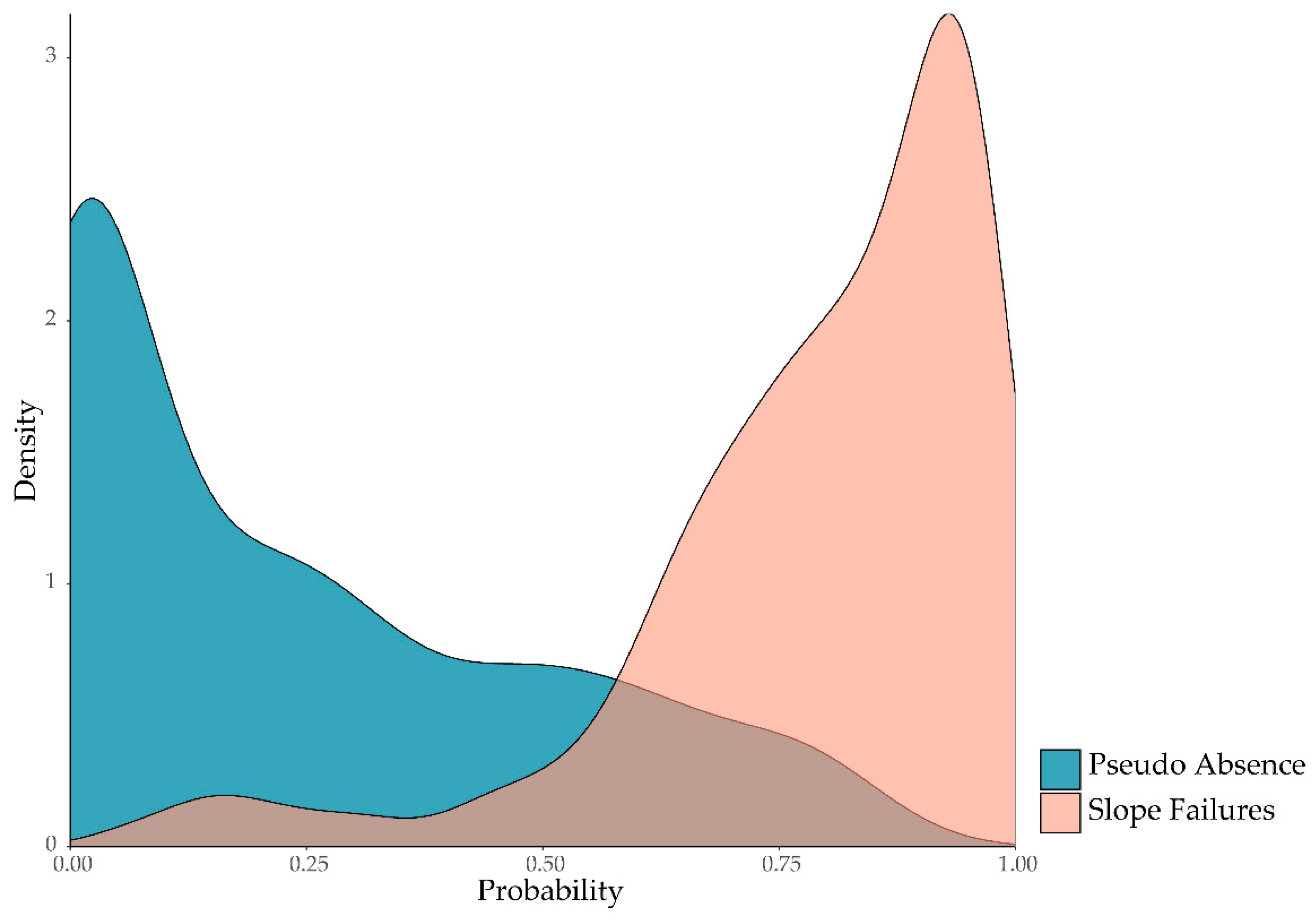
- Does combining multiple models using different sets of pseudo absence data improve slope failure prediction? The use of pseudo absence samples is an approach to generate negative (i.e., no slope failure) examples and is explained in more detail in the Methods section.
- (2).
- Does incorporating additional variables representing lithology, soil characteristics and proximity to roads or streams improve the model in comparison to just using terrain variables?
- (3).
- How does reducing the training sample size impact model performance?
- (4).
- How does predictor variable feature selection impact model performance?
- (5).
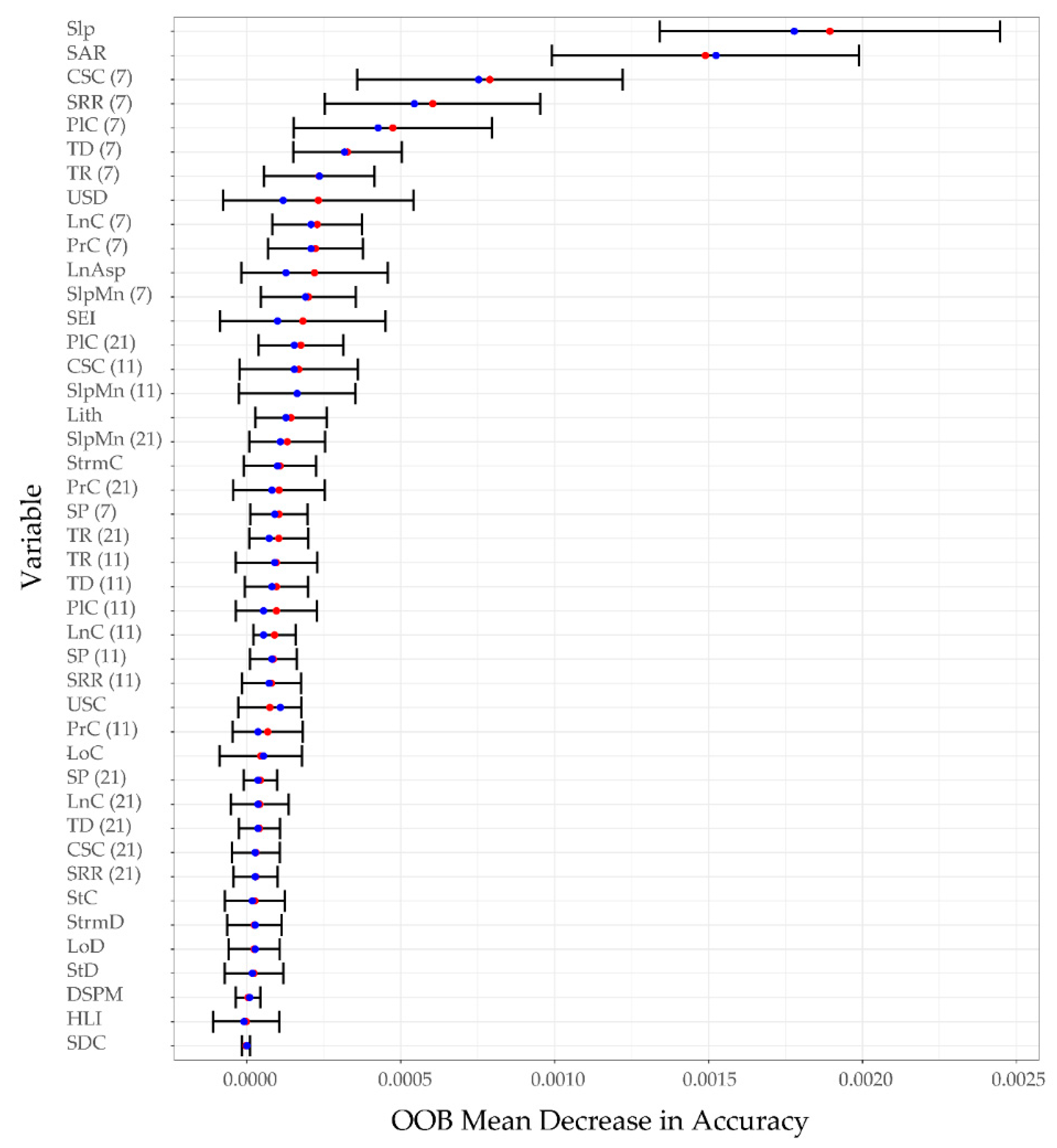
- What variables are most important for predicting slope failure occurrence?
- (6).
- Does calculating terrain variables using multiple window sizes improve the prediction?
1.1. Mapping Slope Failures and Susceptibility
1.2. Random Forest for Spatial Predictive Modeling
1.3. LiDAR and Terrain Variables for Mapping Slope Failures
2. Methods
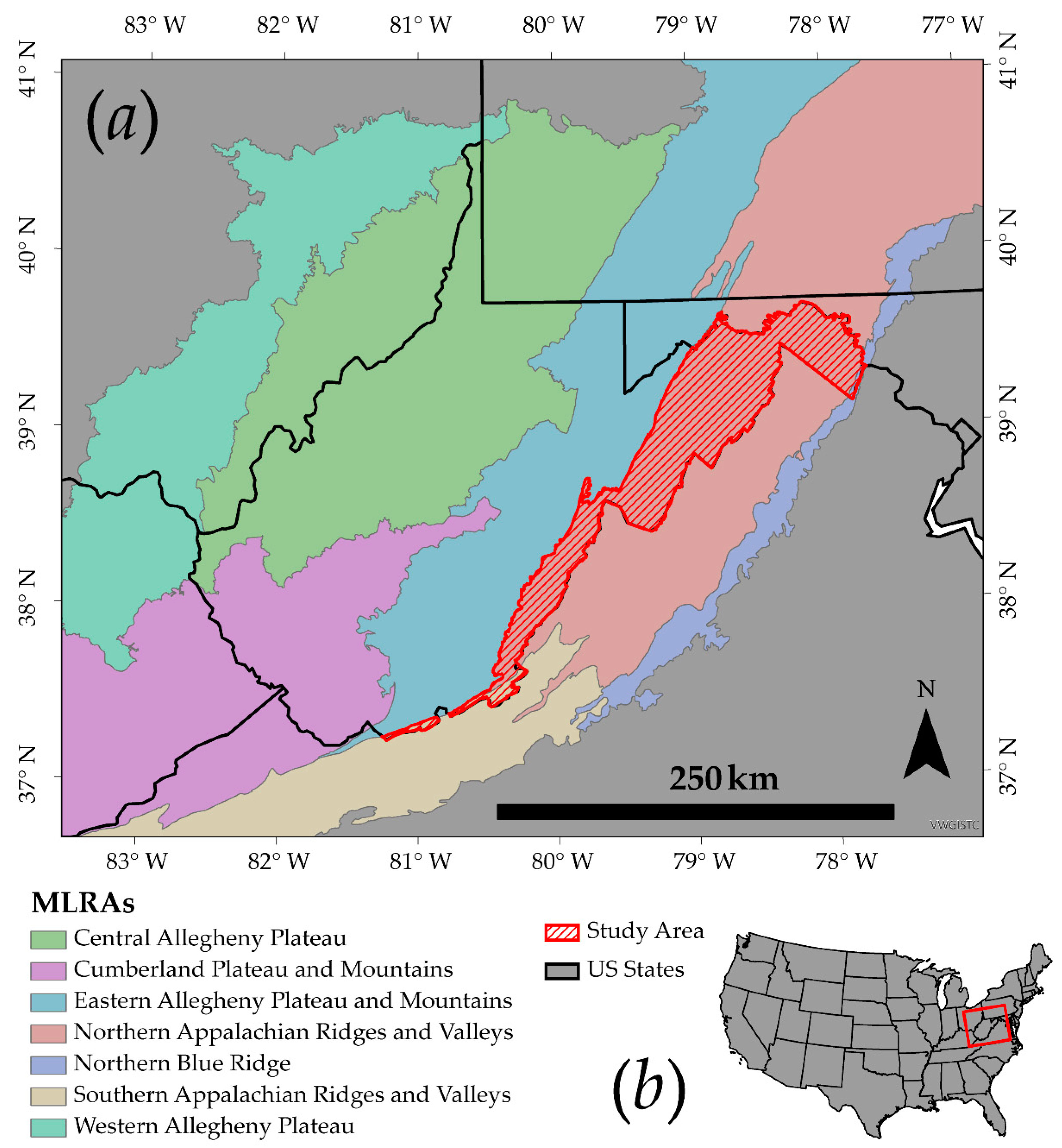
2.1. Study Area
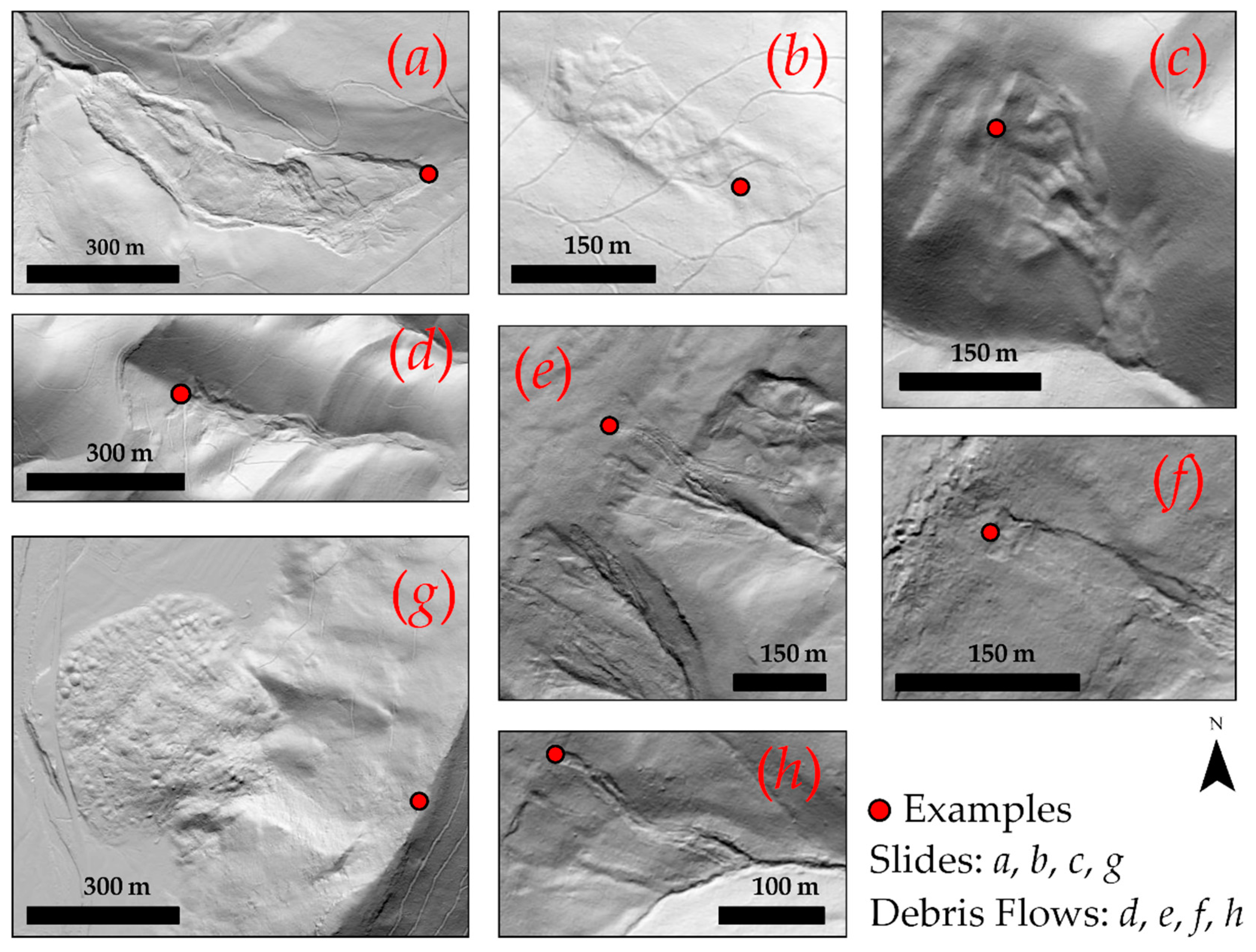
2.2. Reference Data
2.3. Predictor Variables
2.4. RF Modeling and Validation
3. Results
3.1. Impact of Combining Multiple Models
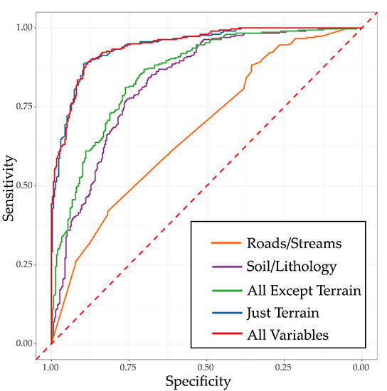
3.2. Removing Variable Groups
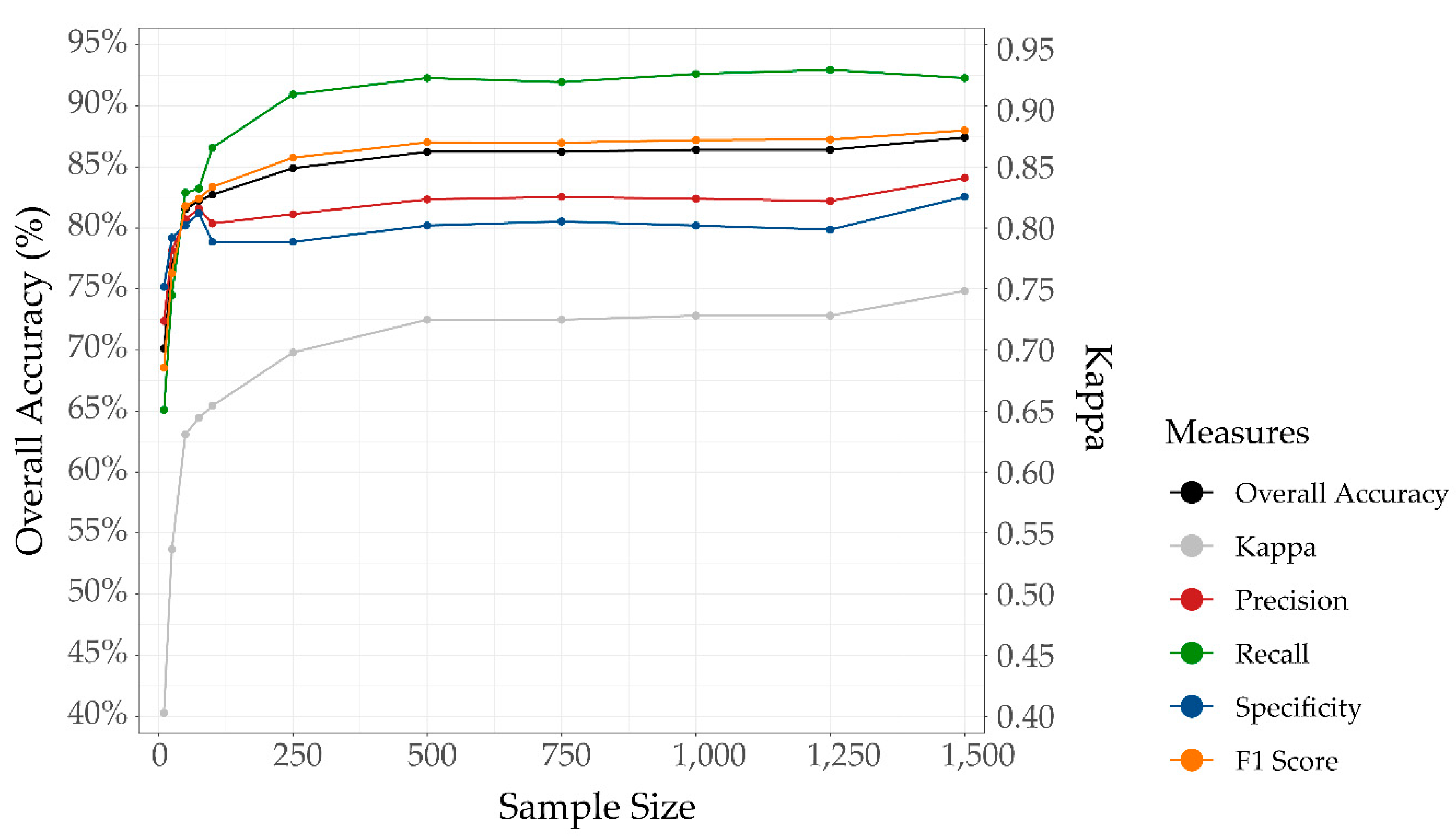
3.3. Impact of Sample Size
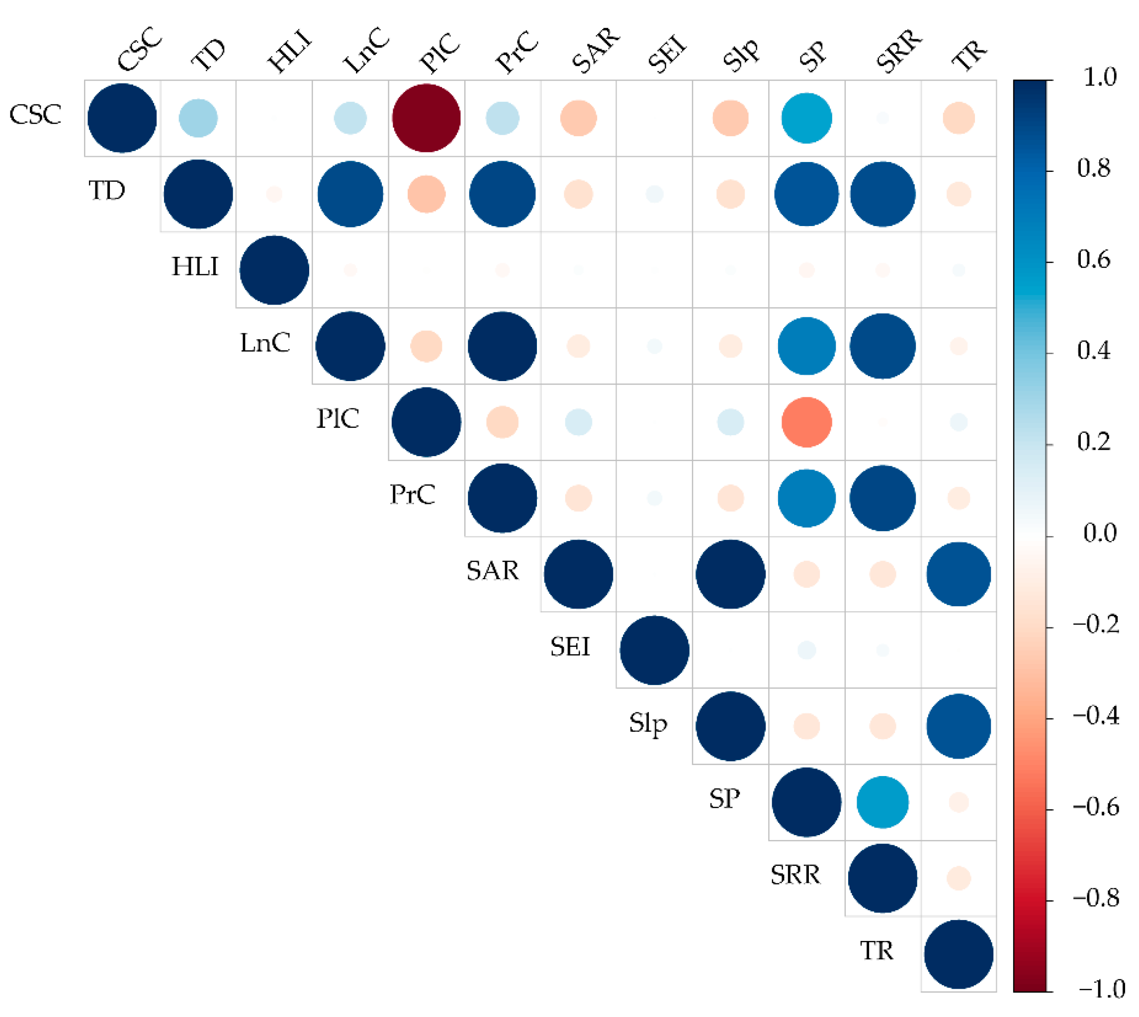
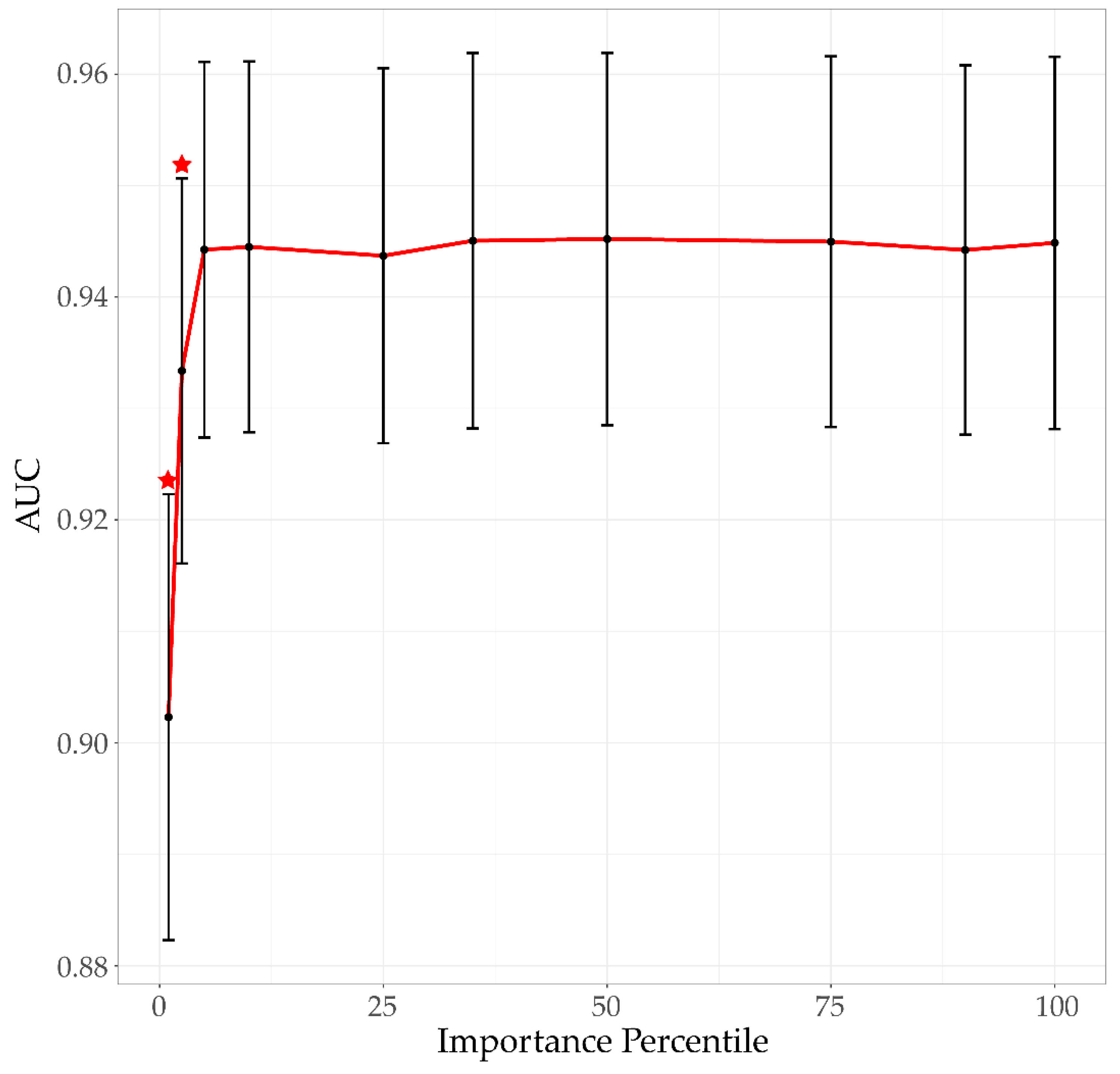
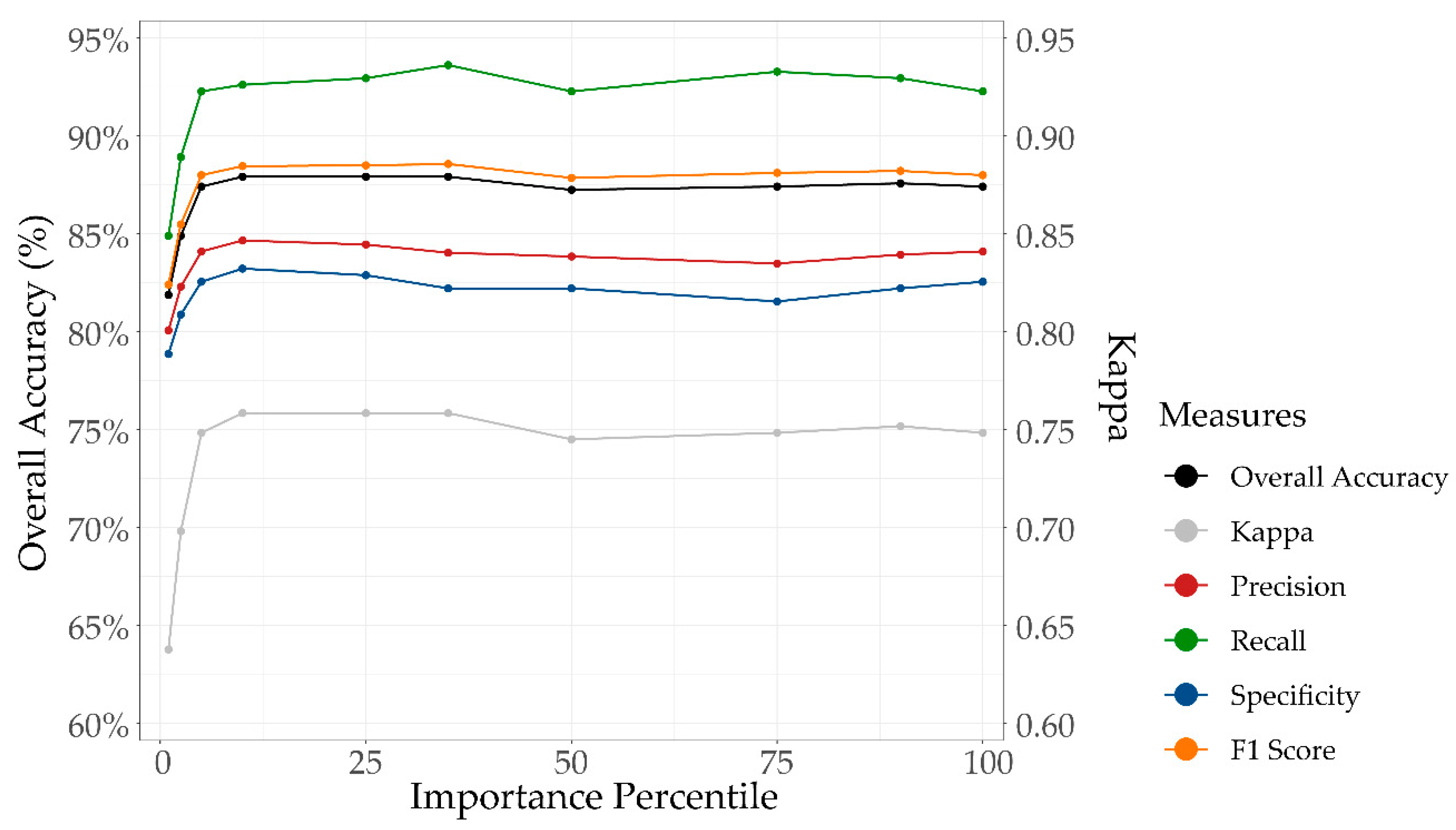
3.4. Feature Reduction and Feature Importance
3.5. Effect of Variable Window Sizes
4. Discussion and Recommendations
5. Conclusions
Author Contributions
Funding
Acknowledgments
Conflicts of Interest
References
- USGS Fact Sheet 2004-3072: Landslide Types and Processes. Available online: https://pubs.usgs.gov/fs/2004/3072/ (accessed on 11 November 2019).
- Landslide Hazards. Available online: https://www.usgs.gov/natural-hazards/landslide-hazards (accessed on 11 November 2019).
- Landslides 101. Available online: https://www.usgs.gov/natural-hazards/landslide-hazards/science/landslides-101?qt-science_center_objects=0#qt-science_center_objects (accessed on 7 November 2019).
- Highland, L.M.; Bobrowsky, P. The Landslide Handbook—A Guide to Understanding Landslides; Circular; U.S. Geological Survey: Reston, VA, USA, 2008; p. 147.
- Petley, D. Global patterns of loss of life from landslides. Geology 2012, 40, 927–930. [Google Scholar] [CrossRef]
- Chiang, S.-H.; Chang, K.-T. The potential impact of climate change on typhoon-triggered landslides in Taiwan, 2010–2099. Geomorphology 2011, 133, 143–151. [Google Scholar] [CrossRef]
- Collison, A.; Wade, S.; Griffiths, J.; Dehn, M. Modelling the impact of predicted climate change on landslide frequency and magnitude in SE England. Eng. Geol. 2000, 55, 205–218. [Google Scholar] [CrossRef]
- Crozier, M.J. Deciphering the effect of climate change on landslide activity: A review. Geomorphology 2010, 124, 260–267. [Google Scholar] [CrossRef]
- Dixon, N.; Brook, E. Impact of predicted climate change on landslide reactivation: Case study of Mam Tor, UK. Landslides 2007, 4, 137–147. [Google Scholar] [CrossRef]
- Jakob, M.; Lambert, S. Climate change effects on landslides along the southwest coast of British Columbia. Geomorphology 2009, 107, 275–284. [Google Scholar] [CrossRef]
- Van Westen, C.J.; Castellanos, E.; Kuriakose, S.L. Spatial data for landslide susceptibility, hazard and vulnerability assessment: An overview. Eng. Geol. 2008, 102, 112–131. [Google Scholar] [CrossRef]
- Carrara, A.; Cardinali, M.; Detti, R.; Guzzetti, F.; Pasqui, V.; Reichenbach, P. GIS techniques and statistical models in evaluating landslide hazard. Earth Surf. Process. Landf. 1991, 16, 427–445. [Google Scholar] [CrossRef]
- Carrara, A.; Sorriso-Valvo, M.; Reali, C. Analysis of landslide form and incidence by statistical techniques, Southern Italy. CATENA 1982, 9, 35–62. [Google Scholar] [CrossRef]
- Carrara, A. Multivariate models for landslide hazard evaluation. Math. Geol. 1983, 15, 403–426. [Google Scholar] [CrossRef]
- Catani, F.; Lagomarsino, D.; Segoni, S.; Tofani, V. Landslide susceptibility estimation by random forests technique: Sensitivity and scaling issues. Nat. Hazards Earth Syst. Sci. 2013, 13, 2815–2831. [Google Scholar] [CrossRef] [Green Version]
- Chen, W.; Pourghasemi, H.R.; Kornejady, A.; Zhang, N. Landslide spatial modeling: Introducing new ensembles of ANN, MaxEnt and SVM machine learning techniques. Geoderma 2017, 305, 314–327. [Google Scholar] [CrossRef]
- Hong, H.; Liu, J.; Bui, D.T.; Pradhan, B.; Acharya, T.D.; Pham, B.T.; Zhu, A.-X.; Chen, W.; Ahmad, B.B. Landslide susceptibility mapping using J48 Decision Tree with AdaBoost, Bagging and Rotation Forest ensembles in the Guangchang area (China). CATENA 2018, 163, 399–413. [Google Scholar] [CrossRef]
- Huang, Y.; Zhao, L. Review on landslide susceptibility mapping using support vector machines. CATENA 2018, 165, 520–529. [Google Scholar] [CrossRef]
- Kim, J.-C.; Lee, S.; Jung, H.-S.; Lee, S. Landslide susceptibility mapping using random forest and boosted tree models in Pyeong-Chang, Korea. Geocarto Int. 2018, 33, 1000–1015. [Google Scholar] [CrossRef]
- Marjanović, M.; Kovačević, M.; Bajat, B.; Voženílek, V. Landslide susceptibility assessment using SVM machine learning algorithm. Eng. Geol. 2011, 123, 225–234. [Google Scholar] [CrossRef]
- Taalab, K.; Cheng, T.; Zhang, Y. Mapping landslide susceptibility and types using Random Forest. Big Earth Data 2018, 2, 159–178. [Google Scholar] [CrossRef]
- Tien Bui, D.; Pradhan, B.; Lofman, O.; Revhaug, I. Landslide Susceptibility Assessment in Vietnam Using Support Vector Machines, Decision Tree and Naïve Bayes Models. Math. Probl. Eng. 2012, 2012, 974638. [Google Scholar] [CrossRef] [Green Version]
- Yao, X.; Tham, L.G.; Dai, F.C. Landslide susceptibility mapping based on Support Vector Machine: A case study on natural slopes of Hong Kong, China. Geomorphology 2008, 101, 572–582. [Google Scholar] [CrossRef]
- Yilmaz, I. Landslide susceptibility mapping using frequency ratio, logistic regression, artificial neural networks and their comparison: A case study from Kat landslides (Tokat—Turkey). Comput. Geosci. 2009, 35, 1125–1138. [Google Scholar] [CrossRef]
- Dou, J.; Yunus, A.P.; Tien Bui, D.; Sahana, M.; Chen, C.-W.; Zhu, Z.; Wang, W.; Thai Pham, B. Evaluating GIS-Based Multiple Statistical Models and Data Mining for Earthquake and Rainfall-Induced Landslide Susceptibility Using the LiDAR DEM. Remote Sens. 2019, 11, 638. [Google Scholar] [CrossRef] [Green Version]
- Ali, I.; Greifeneder, F.; Stamenkovic, J.; Neumann, M.; Notarnicola, C. Review of Machine Learning Approaches for Biomass and Soil Moisture Retrievals from Remote Sensing Data. Remote Sens. 2015, 7, 16398–16421. [Google Scholar] [CrossRef] [Green Version]
- Maxwell, A.E.; Warner, T.A.; Fang, F. Implementation of machine-learning classification in remote sensing: An applied review. Int. J. Remote Sens. 2018, 39, 2784–2817. [Google Scholar] [CrossRef] [Green Version]
- Lary, D.J.; Alavi, A.H.; Gandomi, A.H.; Walker, A.L. Machine learning in geosciences and remote sensing. Geosci. Front. 2016, 7, 3–10. [Google Scholar] [CrossRef] [Green Version]
- Sameen, M.I.; Pradhan, B.; Lee, S. Application of convolutional neural networks featuring Bayesian optimization for landslide susceptibility assessment. CATENA 2020, 186, 104249. [Google Scholar] [CrossRef]
- Wang, Y.; Wang, X.; Jian, J. Remote Sensing Landslide Recognition Based on Convolutional Neural Network. Available online: https://www.hindawi.com/journals/mpe/2019/8389368/ (accessed on 24 January 2020).
- Höfle, B.; Rutzinger, M. Topographic airborne LiDAR in geomorphology: A technological perspective. Z. Geomorphol. Suppl. Issues 2011, 55, 1–29. [Google Scholar] [CrossRef]
- Jaboyedoff, M.; Oppikofer, T.; Abellán, A.; Derron, M.-H.; Loye, A.; Metzger, R.; Pedrazzini, A. Use of LIDAR in landslide investigations: A review. Nat. Hazards 2012, 61, 5–28. [Google Scholar] [CrossRef] [Green Version]
- Passalacqua, P.; Belmont, P.; Staley, D.M.; Simley, J.D.; Arrowsmith, J.R.; Bode, C.A.; Crosby, C.; DeLong, S.B.; Glenn, N.F.; Kelly, S.A.; et al. Analyzing high resolution topography for advancing the understanding of mass and energy transfer through landscapes: A review. Earth-Sci. Rev. 2015, 148, 174–193. [Google Scholar] [CrossRef] [Green Version]
- Migoń, P.; Kasprzak, M.; Traczyk, A. How high-resolution DEM based on airborne LiDAR helped to reinterpret landforms: Examples from the Sudetes, SW Poland. Landf. Anal. 2013, 22. [Google Scholar] [CrossRef]
- Stoker, J.M.; Abdullah, Q.A.; Nayegandhi, A.; Winehouse, J. Evaluation of Single Photon and Geiger Mode Lidar for the 3D Elevation Program. Remote Sens. 2016, 8, 767. [Google Scholar] [CrossRef] [Green Version]
- Arundel, S.T.; Phillips, L.A.; Lowe, A.J.; Bobinmyer, J.; Mantey, K.S.; Dunn, C.A.; Constance, E.W.; Usery, E.L. Preparing The National Map for the 3D Elevation Program—Products, process and research. Cartogr. Geogr. Inf. Sci. 2015, 42, 40–53. [Google Scholar] [CrossRef]
- Kirschbaum, D.B.; Adler, R.; Hong, Y.; Hill, S.; Lerner-Lam, A. A global landslide catalog for hazard applications: Method, results and limitations. Nat. Hazards 2010, 52, 561–575. [Google Scholar] [CrossRef] [Green Version]
- Cruden, D.M. A simple definition of a landslide. Bull. Int. Assoc. Eng. Geol. 1991, 43, 27–29. [Google Scholar] [CrossRef]
- Nichols, J.; Wong, M.S. Satellite remote sensing for detailed landslide inventories using change detection and image fusion. Int. J. Remote Sens. 2005, 26, 1913–1926. [Google Scholar] [CrossRef]
- Lee, S.; Choi, J.; Min, K. Probabilistic landslide hazard mapping using GIS and remote sensing data at Boun, Korea. Int. J. Remote Sens. 2004, 25, 2037–2052. [Google Scholar] [CrossRef]
- Ayalew, L.; Yamagishi, H. The application of GIS-based logistic regression for landslide susceptibility mapping in the Kakuda-Yahiko Mountains, Central Japan. Geomorphology 2005, 65, 15–31. [Google Scholar] [CrossRef]
- Ballabio, C.; Sterlacchini, S. Support Vector Machines for Landslide Susceptibility Mapping: The Staffora River Basin Case Study, Italy. Math. Geosci. 2012, 44, 47–70. [Google Scholar] [CrossRef]
- Casagli, N.; Cigna, F.; Bianchini, S.; Hölbling, D.; Füreder, P.; Righini, G.; Del Conte, S.; Friedl, B.; Schneiderbauer, S.; Iasio, C.; et al. Landslide mapping and monitoring by using radar and optical remote sensing: Examples from the EC-FP7 project SAFER. Remote Sens. Appl. Soc. Environ. 2016, 4, 92–108. [Google Scholar] [CrossRef] [Green Version]
- Colkesen, I.; Sahin, E.K.; Kavzoglu, T. Susceptibility mapping of shallow landslides using kernel-based Gaussian process, support vector machines and logistic regression. J. Afr. Earth Sci. 2016, 118, 53–64. [Google Scholar] [CrossRef]
- Goetz, J.N.; Brenning, A.; Petschko, H.; Leopold, P. Evaluating machine learning and statistical prediction techniques for landslide susceptibility modeling. Comput. Geosci. 2015, 81, 1–11. [Google Scholar] [CrossRef]
- Lee, S. Application of logistic regression model and its validation for landslide susceptibility mapping using GIS and remote sensing data. Int. J. Remote Sens. 2005, 26, 1477–1491. [Google Scholar] [CrossRef]
- Lu, P.; Stumpf, A.; Kerle, N.; Casagli, N. Object-Oriented Change Detection for Landslide Rapid Mapping. IEEE Geosci. Remote Sens. Lett. 2011, 8, 701–705. [Google Scholar] [CrossRef]
- Lee, S.; Ryu, J.-H.; Won, J.-S.; Park, H.-J. Determination and application of the weights for landslide susceptibility mapping using an artificial neural network. Eng. Geol. 2004, 71, 289–302. [Google Scholar] [CrossRef]
- Pradhan, B. A comparative study on the predictive ability of the decision tree, support vector machine and neuro-fuzzy models in landslide susceptibility mapping using GIS. Comput. Geosci. 2013, 51, 350–365. [Google Scholar] [CrossRef]
- Sarkar, S.; Kanungo, D.P. An Integrated Approach for Landslide Susceptibility Mapping Using Remote Sensing and GIS. Photogramm. Eng. Remote Sens. 2004, 70, 617–625. [Google Scholar] [CrossRef]
- Stumpf, A.; Kerle, N. Object-oriented mapping of landslides using Random Forests. Remote Sens. Environ. 2011, 115, 2564–2577. [Google Scholar] [CrossRef]
- Stumpf, A.; Kerle, N. Combining Random Forests and object-oriented analysis for landslide mapping from very high resolution imagery. Procedia Environ. Sci. 2011, 3, 123–129. [Google Scholar] [CrossRef] [Green Version]
- Liu, Y.; Wu, L. Geological Disaster Recognition on Optical Remote Sensing Images Using Deep Learning. Procedia Comput. Sci. 2016, 91, 566–575. [Google Scholar] [CrossRef] [Green Version]
- Trigila, A.; Iadanza, C.; Esposito, C.; Scarascia-Mugnozza, G. Comparison of Logistic Regression and Random Forests techniques for shallow landslide susceptibility assessment in Giampilieri (NE Sicily, Italy). Geomorphology 2015, 249, 119–136. [Google Scholar] [CrossRef]
- Youssef, A.M.; Pourghasemi, H.R.; Pourtaghi, Z.S.; Al-Katheeri, M.M. Landslide susceptibility mapping using random forest, boosted regression tree, classification and regression tree and general linear models and comparison of their performance at Wadi Tayyah Basin, Asir Region, Saudi Arabia. Landslides 2016, 13, 839–856. [Google Scholar] [CrossRef]
- Ghorbanzadeh, O.; Meena, S.R.; Blaschke, T.; Aryal, J. UAV-Based Slope Failure Detection Using Deep-Learning Convolutional Neural Networks. Remote Sens. 2019, 11, 2046. [Google Scholar] [CrossRef] [Green Version]
- Ghorbanzadeh, O.; Blaschke, T.; Gholamnia, K.; Meena, S.R.; Tiede, D.; Aryal, J. Evaluation of Different Machine Learning Methods and Deep-Learning Convolutional Neural Networks for Landslide Detection. Remote Sens. 2019, 11, 196. [Google Scholar] [CrossRef] [Green Version]
- Jin, K.P.; Yao, L.K.; Cheng, Q.G.; Xing, A.G. Seismic landslides hazard zoning based on the modified Newmark model: A case study from the Lushan earthquake, China. Nat. Hazards 2019, 99, 493–509. [Google Scholar] [CrossRef]
- Lei, T.; Zhang, Q.; Xue, D.; Chen, T.; Meng, H.; Nandi, A.K. End-to-end Change Detection Using a Symmetric Fully Convolutional Network for Landslide Mapping. In Proceedings of the ICASSP 2019–2019 IEEE International Conference on Acoustics, Speech and Signal Processing (ICASSP), Brighton, UK, 12–17 May 2019; pp. 3027–3031. [Google Scholar]
- Lei, T.; Zhang, Y.; Lv, Z.; Li, S.; Liu, S.; Nandi, A.K. Landslide Inventory Mapping From Bitemporal Images Using Deep Convolutional Neural Networks. IEEE Geosci. Remote Sens. Lett. 2019, 16, 982–986. [Google Scholar] [CrossRef]
- Reichenbach, P.; Rossi, M.; Malamud, B.D.; Mihir, M.; Guzzetti, F. A review of statistically-based landslide susceptibility models. Earth-Sci. Rev. 2018, 180, 60–91. [Google Scholar] [CrossRef]
- Breiman, L. Random Forests. Mach. Learn. 2001, 45, 5–32. [Google Scholar] [CrossRef] [Green Version]
- Pal, M.; Mather, P.M. An assessment of the effectiveness of decision tree methods for land cover classification. Remote Sens. Environ. 2003, 86, 554–565. [Google Scholar] [CrossRef]
- Ghimire, B.; Rogan, J.; Galiano, V.R.; Panday, P.; Neeti, N. An Evaluation of Bagging, Boosting and Random Forests for Land-Cover Classification in Cape Cod, Massachusetts, USA. GISci. Remote Sens. 2012, 49, 623–643. [Google Scholar] [CrossRef]
- Evans, J.S.; Cushman, S.A. Gradient modeling of conifer species using random forests. Landsc. Ecol. 2009, 24, 673–683. [Google Scholar] [CrossRef]
- Gislason, P.O.; Benediktsson, J.A.; Sveinsson, J.R. Random Forest classification of multisource remote sensing and geographic data. In Proceedings of the IGARSS 2004, 2004 IEEE International Geoscience and Remote Sensing Symposium, Anchorage, AK, USA, 20–24 September 2004; Volume 2, pp. 1049–1052. [Google Scholar]
- Gislason, P.O.; Benediktsson, J.A.; Sveinsson, J.R. Random Forests for land cover classification. Pattern Recognit. Lett. 2006, 27, 294–300. [Google Scholar] [CrossRef]
- Pourghasemi, H.R.; Kerle, N. Random forests and evidential belief function-based landslide susceptibility assessment in Western Mazandaran Province, Iran. Environ. Earth Sci. 2016, 75, 185. [Google Scholar] [CrossRef]
- Maxwell, A.E.; Warner, T.A.; Strager, M.P. Predicting Palustrine Wetland Probability Using Random Forest Machine Learning and Digital Elevation Data-Derived Terrain Variables. Available online: https://www.ingentaconnect.com/content/asprs/pers/2016/00000082/00000006/art00016 (accessed on 12 November 2019).
- Strager, M.P.; Strager, J.M.; Evans, J.S.; Dunscomb, J.K.; Kreps, B.J.; Maxwell, A.E. Combining a Spatial Model and Demand Forecasts to Map Future Surface Coal Mining in Appalachia. PLoS ONE 2015, 10, e0128813. [Google Scholar] [CrossRef] [PubMed]
- Lillesand, T.; Kiefer, R.W.; Chipman, J. Remote Sensing and Image Interpretation, 7th ed.; Wiley: Hoboken, NJ, USA, 2015; Available online: https://www.wiley.com/en-us/Remote+Sensing+and+Image+Interpretation%2C+7th+Edition-p-9781118343289 (accessed on 28 October 2019).
- Goetz, J.N.; Guthrie, R.H.; Brenning, A. Integrating physical and empirical landslide susceptibility models using generalized additive models. Geomorphology 2011, 129, 376–386. [Google Scholar] [CrossRef]
- Mahalingam, R.; Olsen, M.J.; O’Banion, M.S. Evaluation of landslide susceptibility mapping techniques using lidar-derived conditioning factors (Oregon case study). Geomat. Nat. Hazards Risk 2016, 7, 1884–1907. [Google Scholar] [CrossRef]
- Huisman, O. Principles of Geographic Information Systems—An Introductory Textbook. Available online: https://webapps.itc.utwente.nl/librarywww/papers_2009/general/principlesgis.pdf (accessed on 28 January 2020).
- Gessler, P.E.; Moore, I.D.; McKenzie, N.J.; Ryan, P.J. Soil-landscape modelling and spatial prediction of soil attributes. Int. J. Geogr. Inf. Syst. 1995, 9, 421–432. [Google Scholar] [CrossRef]
- Moore, I.D.; Grayson, R.B.; Ladson, A.R. Digital terrain modelling: A review of hydrological, geomorphological and biological applications. Hydrol. Process. 1991, 5, 3–30. [Google Scholar] [CrossRef]
- Zevenbergen, L.W.; Thorne, C.R. Quantitative analysis of land surface topography. Earth Surf. Process. Landf. 1987, 12, 47–56. [Google Scholar] [CrossRef]
- Maxwell, A.E.; Warner, T.A. Is high spatial resolution DEM data necessary for mapping palustrine wetlands? Int. J. Remote Sens. 2019, 40, 118–137. [Google Scholar] [CrossRef]
- Nusser, S.M.; Goebel, J.J. The National Resources Inventory: A long-term multi-resource monitoring programme. Environ. Ecol. Stat. 1997, 4, 181–204. [Google Scholar] [CrossRef]
- Landslide Susceptibility Pilot Study_BerkleyCounty_20160408.pdf. Available online: http://data.wvgis.wvu.edu/pub/temp/Landslide/Landslide%20Susceptibility%20Pilot%20Study_BerkleyCounty_20160408.pdf (accessed on 28 January 2020).
- Cardwell, D.H.; Erwin, R.B.; Woodward, H.P. Geologic Map of West Virginia; West Virginia Geological and Economic Survey: Morgantown, WV, USA, 1968. [Google Scholar]
- Strausbaugh, P.D.; Core, E.L. Flora of West Virginia; West Virginia University Bulletin: Morgantown, WV, USA, 1952. [Google Scholar]
- WVGES: WV Physiographic Provinces. Available online: https://www.wvgs.wvnet.edu/www/maps/pprovinces.htm (accessed on 14 November 2019).
- Chang, K.-T. Geographic Information System. In International Encyclopedia of Geography; American Cancer Society: Atlanta, GA, USA, 2017; pp. 1–9. ISBN 978-1-118-78635-2. [Google Scholar]
- Reed, M. How Will Anthropogenic Valley Fills in Appalachian Headwaters Erode? MS, West Virginia University Libraries: Morgantown, WV, USA, 2018. [Google Scholar]
- ArcGIS, version Pro 2.2; Software for Technical Computation; ESRI: Redlands, CA, USA, 2018.
- ArcGIS Gradient Metrics Toolbox. Available online: https://evansmurphy.wixsite.com/evansspatial/arcgis-gradient-metrics-toolbox (accessed on 14 November 2019).
- SAGA—System for Automated Geoscientific Analyses. Available online: http://www.saga-gis.org/en/index.html (accessed on 14 November 2019).
- Module Morphometric Features/SAGA-GIS Module Library Documentation (v2.2.5). Available online: http://www.saga-gis.org/saga_tool_doc/2.2.5/ta_morphometry_23.html (accessed on 14 November 2019).
- Wood, J. Chapter 14 Geomorphometry in LandSerf. In Developments in Soil Science; Hengl, T., Reuter, H.I., Eds.; Geomorphometry; Elsevier: Amsterdam, The Netherlands, 2009; Volume 33, pp. 333–349. [Google Scholar]
- Wood, J. The Geomorphological Characterisation of Digital Elevation Models. Ph.D. Thesis, University of Leicester, Leicester, UK, 1996. [Google Scholar]
- Albani, M.; Klinkenberg, B.; Andison, D.W.; Kimmins, J.P. The choice of window size in approximating topographic surfaces from Digital Elevation Models. Int. J. Geogr. Inf. Sci. 2004, 18, 577–593. [Google Scholar] [CrossRef]
- Hengl, T.; Gruber, S.; Shrestha, D.P. Reduction of errors in digital terrain parameters used in soil-landscape modelling. Int. J. Appl. Earth Obs. Geoinf. 2004, 5, 97–112. [Google Scholar] [CrossRef]
- Franklin, S.E. Geomorphometric processing of digital elevation models. Comput. Geosci. 1987, 13, 603–609. [Google Scholar] [CrossRef]
- Wilson, J.P.; Gallant, J.C. Terrain Analysis: Principles and Applications; John Wiley & Sons: Hoboken, NJ, USA, 2000; ISBN 978-0-471-32188-0. [Google Scholar]
- Moreno, M.; Levachkine, S.; Torres, M.; Quintero, R. Geomorphometric Analysis of Raster Image Data to detect Terrain Ruggedness and Drainage Density. In Progress in Pattern Recognition, Speech and Image Analysis; Sanfeliu, A., Ruiz-Shulcloper, J., Eds.; Springer: Berlin/Heidelberg, Germany, 2003; pp. 643–650. [Google Scholar]
- Evans, I.S.; Minár, J. A classification of geomorphometric variables. Int. Geom-Orphometry 2011, 4, 105–108. [Google Scholar]
- Jenness, J.S. Calculating Landscape Surface Area from Digital Elevation Models. Wildl. Soc. Bull. 2004, 32, 829–839. [Google Scholar] [CrossRef]
- Pike, R.J.; Wilson, S.E. Elevation-Relief Ratio, Hypsometric Integral and Geomorphic Area-Altitude Analysis. GSA Bull. 1971, 82, 1079–1084. [Google Scholar] [CrossRef]
- Balice, R.G.; Miller, J.D.; Oswald, B.P.; Edminster, C.; Yool, S.R. Forest Surveys and Wildfire Assessment in the Los Alamos Region, 1998–1999; Los Alamos National Lab.: New Mexico, NM, USA, 2000.
- McCune, B.; Keon, D. Equations for potential annual direct incident radiation and heat load. J. Veg. Sci. 2002, 13, 603–606. [Google Scholar] [CrossRef]
- SSURGO|NRCS Soils. Available online: https://www.nrcs.usda.gov/wps/portal/nrcs/detail/soils/survey/office/ssr12/tr/?cid=nrcs142p2_010596 (accessed on 14 November 2019).
- Liaw, A.; Wiener, M. Classification and Regression by randomForest. R News 2002, 2, 6. [Google Scholar]
- R Core Team. R: A Language and Environment for Statistical Computing; R Foundation for Statistical Computing: Vienna, Austria, 2018. [Google Scholar]
- Strobl, C.; Hothorn, T.; Zeileis, A. Party on! A new, conditional variable importance measure available in the party package. R J. 2009, 1, 14–17. [Google Scholar] [CrossRef]
- Conditional Variable Importance for Random Forests|BMC Bioinformatics|Full Text. Available online: https://bmcbioinformatics.biomedcentral.com/articles/10.1186/1471-2105-9-307 (accessed on 15 November 2019).
- Spearman, C. The proof and measurement of association between two things. Int. J. Epidemiol. 2010, 39, 1137–1150. [Google Scholar] [CrossRef] [Green Version]
- Beck, J.R.; Shultz, E.K. The use of relative operating characteristic (ROC) curves in test performance evaluation. Arch. Pathol. Lab. Med. 1986, 110, 13–20. [Google Scholar]
- Robin, X.; Turck, N.; Hainard, A.; Tiberti, N.; Lisacek, F.; Sanchez, J.-C.; Müller, M. pROC: An open-source package for R and S+ to analyze and compare ROC curves. BMC Bioinform. 2011, 12, 77. [Google Scholar] [CrossRef] [PubMed]
- A Method of Comparing the Areas under Receiver Operating Characteristic Curves Derived from the Same Cases. | Radiology. Available online: https://pubs.rsna.org/doi/abs/10.1148/radiology.148.3.6878708 (accessed on 15 November 2019).
- DeLong, E.R.; DeLong, D.M.; Clarke-Pearson, D.L. Comparing the Areas under Two or More Correlated Receiver Operating Characteristic Curves: A Nonparametric Approach. Biometrics 1988, 44, 837–845. [Google Scholar] [CrossRef] [PubMed]
- Saito, T.; Rehmsmeier, M. The Precision-Recall Plot Is More Informative than the ROC Plot When Evaluating Binary Classifiers on Imbalanced Datasets. PLoS ONE 2015, 10, e0118432. [Google Scholar] [CrossRef] [PubMed] [Green Version]
- Grau, J.; Grosse, I.; Keilwagen, J. PRROC: Computing and visualizing precision-recall and receiver operating characteristic curves in R. Bioinformatics 2015, 31, 2595–2597. [Google Scholar] [CrossRef] [PubMed]
- Keilwagen, J.; Grosse, I.; Grau, J. Area under Precision-Recall Curves for Weighted and Unweighted Data. PLoS ONE 2014, 9, e92209. [Google Scholar] [CrossRef] [PubMed]
- Maxwell, A.E.; Strager, M.P.; Warner, T.A.; Ramezan, C.A.; Morgan, A.N.; Pauley, C.E. Large-Area, High Spatial Resolution Land Cover Mapping Using Random Forests, GEOBIA and NAIP Orthophotography: Findings and Recommendations. Remote Sens. 2019, 11, 1409. [Google Scholar] [CrossRef] [Green Version]


| Study 2 | Terrain Variables | Year | Algorithm(s) |
|---|---|---|---|
| Lee et al. | Curvature (non-directional), Slope | 2004 | LR |
| Ayalew and Yamagishi | Aspect, Elevation, Slope | 2005 | LR |
| Lee | Aspect, Curvature (non-directional), Slope | 2005 | LR |
| Yao et al. | Aspect, Curvature (Profile), Elevation, Slope, TWI | 2008 | SVM |
| Yilmaz | Aspect, Elevation, Slope, SPI, TWI | 2009 | ANN, FR, LR |
| Marjanović et al. | Aspect, Curvature (Plan), Curvature (Profile), Elevation, Slope, Slope Length, TWI | 2011 | SVM |
| Ballabio and Sterlacchini | CBL, CI, Downslope Distance Gradient, Elevation, HLI, Internal Relief, MPI, Slope, SPI, TWI | 2012 | SVM |
| Tien et al. | Aspect, Relief Amplitude, Slope | 2012 | DT, NB, SVM |
| Catani et al. | Aspect, Curvature (Plan), Curvature (Profile), Curvature (Classified), FA, Second Derivative of Elevation, Slope, TWI | 2013 | RF |
| Pradhan | Curvature (Plan), Elevation, Slope, TWI | 2013 | ANN, DT, SVM |
| Goetz et al. | Aspect, Curvature (Plan), Curvature (Profile), CH, CI, Elevation, FA, Slope, TR, TWI | 2015 | BPLDA, GAM, GLM, RF, SVM, WOE |
| Trigila et al. | Aspect, Curvature (non-directional), Curvature (Plan), Curvature (Profile), FA, Slope, SPI | 2015 | LR, RF |
| Mahalingam et al. | Slope, SPI, SR, TR, TWI | 2016 | ANN, DA, FR, LR, SVM, WOE |
| Pourghasemi and Kerle | Aspect, CTMI, Curvature (Plan), Curvature (Profile), Elevation, Slope, TWI | 2016 | RF |
| Youssef et al. | Aspect, Curvature (Plan), Curvature (Profile), Elevation, Slope | 2016 | Boosted DT, DT, GLM, RF |
| Chen et al. | Aspect, Curvature (Profile), Curvature (Plan), Elevation, Slope, TWI | 2017 | ANN, Maxent, SVM, Ensemble of methods |
| Hong et al. | Aspect, Curvature (Plan), Curvature (Profile), Elevation, Slope, SPI, STI, TWI | 2018 | Boosted DT, DT, RF |
| Kim et al. | Aspect, Curvature (non-directional), Slope, SPI, TWI | 2018 | Boosted DT, RF |
| Taalab et al. | Aspect, CTMI, Curvature (non-directional), Curvature (Plan), Curvature (Profile), Landform, Slope, TWI | 2018 | RF |
| Dou et al. | Aspect, Curvature (Plan), Drainage Density, Elevation, Slope | 2019 | ANN, CF, InV, PLFR, SVM |
| Variable 1 | Abbreviation | Description 2 | Window Radius 3 (Cells) |
|---|---|---|---|
| Slope Gradient | Slp | Gradient or rate of maximum change in Z as degrees of rise | 1 |
| Mean Slope Gradient | SlpMn | Slope averaged over a local window | 7, 11, 21 |
| Linear Aspect | LnAsp | Transform of topographic aspect to linear variable | 1 |
| Profile Curvature | PrC | Curvature parallel to direction of maximum slope | 7, 11, 21 |
| Plan Curvature | Plc | Curvature perpendicular to direction of maximum slope | 7, 11, 21 |
| Longitudinal Curvature | LnC | Profile curvature intersecting with the plane defined by the surface normal and maximum gradient direction | 7, 11, 21 |
| Cross-Sectional Curvature | CSC | Tangential curvature intersecting with the plane defined by the surface normal and a tangent to the contour - perpendicular to maximum gradient direction | 7, 11, 21 |
| Slope Position | SP | Z – Mean Z | 7, 11, 21 |
| Topographic Roughness | TR | Square root of standard deviation of slope in local window | 7, 11, 21 |
| Topographic Dissection | TD | 7, 11, 21 | |
| Surface Area Ratio | SAR | 1 | |
| Surface Relief Ratio | SRR | 7, 11, 21 | |
| Site Exposure Index | SEI | Measure of exposure based on slope and aspect | 1 |
| Heat Load Index | HLI | Measure of solar insolation based on slope, aspect and latitude | 1 |
| Variable | Abbreviation | Description |
|---|---|---|
| Distance to Roads (US, state and local) | USD, StD, LoD | Euclidean distance to nearest US, state or local road |
| Cost Distance to US Roads (US, state and local) | USC, StC, LoC | Euclidean distance to nearest US, state or local road weighted by slope |
| Distance from Streams | StrmD | Distance from mapped streams |
| Cost Distance from Streams | StrmC | Distance from mapped streams weighted by slope |
| Geomorphic Presentation | Lith | Classification of rock formations based on geomorphic presentation |
| Dominant Soil Parent Material | DSPM | Dominant parent material of soil |
| Soil Drainage Class | SDC | Drainage class of soil |
| Geomorphic Presentation (Lith) | Dominant Soil Parent Material (DSPM) | Soil Drainage Class (SDC) |
|---|---|---|
| Low relief carbonates | Colluvium | Excessively drained |
| Low relief mudrock | Disturbed areas | Somewhat excessively drained |
| Major ridge formers | Lacustrine | Well drained |
| Moderate or variable quartzose ridge formers | Marl | Moderately well drained |
| Moderate relief clastic rocks | Mine regolith | Somewhat poorly drained |
| Other | Old alluvium | Poorly drained |
| Shaley units with interbedded sandstone | Recent alluvium | Very poorly drained |
| Variable low ridge or hill forming carbonates with chert or sandstone | Residuum, acid clastic | |
| Residuum, calcareous clastic | ||
| Residuum, Limestone | ||
| Residuum, metamorphic/igneous | ||
| Water |
| Model 1 | Model 2 | Model 3 | Model 4 | Model 5 | Combined | |
|---|---|---|---|---|---|---|
| AUC | 0.945 | 0.942 | 0.942 | 0.946 | 0.940 | 0.946 |
| AUC Lower | 0.928 | 0.925 | 0.926 | 0.925 | 0.924 | 0.930 |
| AUC Upper | 0.962 | 0.958 | 0.959 | 0.959 | 0.957 | 0.962 |
| AUC (PRC) | 0.945 | 0.943 | 0.945 | 0.944 | 0.942 | 0.949 |
| Kappa | 0.748 | 0.748 | 0.738 | 0.738 | 0.715 | 0.742 |
| Overall Accuracy | 87.4% | 87.4% | 86.9% | 86.9% | 85.7% | 87.1% |
| Precision | 0.839 | 0.833 | 0.831 | 0.831 | 0.816 | 0.834 |
| Recall | 0.926 | 0.936 | 0.926 | 0.926 | 0.923 | 0.926 |
| Specificity | 0.822 | 0.812 | 0.812 | 0.812 | 0.792 | 0.815 |
| F1 Score | 0.880 | 0.882 | 0.876 | 0.876 | 0.866 | 0.878 |
| Model 1 | ||||||
| Model 2 | ||||||
| Model 3 | ||||||
| Model 4 | ||||||
| Model 5 | X | |||||
| Combined |
| Soil/Lithology | Roads/Streams | All Except Terrain | Just Terrain | All Variables | |
|---|---|---|---|---|---|
| Number of Variables | 3 | 8 | 11 | 32 | 43 |
| AUC | 0.677 | 0.830 | 0.856 | 0.944 | 0.946 |
| AUC Lower | 0.656 | 0.807 | 0.834 | 0.927 | 0.930 |
| AUC Upper | 0.698 | 0.853 | 0.878 | 0.961 | 0.962 |
| AUC (PRC) | 0.661 | 0.791 | 0.838 | 0.946 | 0.949 |
| Kappa | 0.218 | 0.527 | 0.560 | 0.732 | 0.742 |
| Overall Accuracy | 60.9% | 76.3% | 78.0% | 86.6% | 87.1% |
| Precision | 0.572 | 0.728 | 0.738 | 0.830 | 0.834 |
| Recall | 0.862 | 0.842 | 0.869 | 0.919 | 0.926 |
| Specificity | 0.356 | 0.685 | 0.691 | 0.812 | 0.815 |
| F1 Score | 0.688 | 0.781 | 0.798 | 0.873 | 0.878 |
| Soil/Lithology | X | X | X | X | |
| Roads/Streams | X | X | X | ||
| All Except Terrain | X | X | |||
| Just Terrain | |||||
| All Variables |
| 7 | 11 | 21 | All Sizes | |
|---|---|---|---|---|
| AUC | 0.941 | 0.937 | 0.922 | 0.944 |
| AUC Upper | 0.924 | 0.920 | 0.904 | 0.927 |
| AUC Lower | 0.958 | 0.955 | 0.941 | 0.961 |
| AUC (PRC) | 0.942 | 0.940 | 0.922 | 0.947 |
| Kappa | 0.721 | 0.735 | 0.688 | 0.735 |
| Overall Accuracy | 86.1% | 86.7% | 84.4% | 86.7% |
| Precision | 0.821 | 0.837 | 0.812 | 0.831 |
| Recall | 0.923 | 0.913 | 0.896 | 0.923 |
| Specificity | 0.799 | 0.822 | 0.792 | 0.812 |
| F1 Score | 0.869 | 0.873 | 0.852 | 0.874 |
| 7 | X | |||
| 11 | X | |||
| 21 | X | |||
| All Sizes |
© 2020 by the authors. Licensee MDPI, Basel, Switzerland. This article is an open access article distributed under the terms and conditions of the Creative Commons Attribution (CC BY) license (http://creativecommons.org/licenses/by/4.0/).
Share and Cite
Maxwell, A.E.; Sharma, M.; Kite, J.S.; Donaldson, K.A.; Thompson, J.A.; Bell, M.L.; Maynard, S.M. Slope Failure Prediction Using Random Forest Machine Learning and LiDAR in an Eroded Folded Mountain Belt. Remote Sens. 2020, 12, 486. https://doi.org/10.3390/rs12030486
Maxwell AE, Sharma M, Kite JS, Donaldson KA, Thompson JA, Bell ML, Maynard SM. Slope Failure Prediction Using Random Forest Machine Learning and LiDAR in an Eroded Folded Mountain Belt. Remote Sensing. 2020; 12(3):486. https://doi.org/10.3390/rs12030486
Chicago/Turabian StyleMaxwell, Aaron E., Maneesh Sharma, James S. Kite, Kurt A. Donaldson, James A. Thompson, Matthew L. Bell, and Shannon M. Maynard. 2020. "Slope Failure Prediction Using Random Forest Machine Learning and LiDAR in an Eroded Folded Mountain Belt" Remote Sensing 12, no. 3: 486. https://doi.org/10.3390/rs12030486