Coast–Ship Bistatic HF Surface Wave Radar: Simulation Analysis and Experimental Verification
by
 , ,
, ,
Yonggang Ji
1,* ,
,
Jie Zhang
1, 
Yiming Wang
1,
Chao Yue
1,
Weichun Gong
1,
Junwei Liu
1,
Hao Sun
1,
Changjun Yu
2 and
Ming Li
3 1
Laboratory of Marine Physics and Remote Sensing, First Institute of Oceanography, Ministry of Natural Resources, No. 6 Xianxialing Road, Qingdao 266061, China
2
School of Information and Electrical Engineering, Harbin Institute of Technology at Weihai, Weihai 264209, China
3
College of Engineering, Ocean University of China, Qingdao, Shandong 266100, China
*
Author to whom correspondence should be addressed.
Remote Sens. 2020, 12(3), 470; https://doi.org/10.3390/rs12030470
Submission received: 29 November 2019
/
Revised: 29 January 2020
/
Accepted: 31 January 2020
/
Published: 2 February 2020
(This article belongs to the Special Issue Bistatic HF Radar)
Abstract
:The coast–ship bistatic high-frequency surface wave radar (HFSWR) not only has the anti-interference advantages of the coast-based bistatic HFSWR, but also has the advantages of maneuverability and an extended detection area of the shipborne HFSWR. In this paper, theoretical formulas were derived for the coast–ship bistatic radar, including the first-order sea clutter scattering cross-section and the Doppler frequency shift of moving targets. Then, simulation results of the first-order sea clutter spectrum under different operating conditions were given, and the range of broadening of the first-order sea clutter spectrum and its influence on target detection were investigated. The simulation results show the broadening ranges of the right sea clutter spectrum and left sea clutter spectrum were symmetric when the shipborne platform was anchored, whereas they were asymmetric when the shipborne platform was underway. This asymmetry is primarily a function of platform velocity and radar frequency. Based on experimental data of the coast–ship bistatic HFSWR conducted in 2019, the broadening range of the sea clutter and the target frequency shift were analyzed and compared with simulation results based on the same parameter configuration. The agreement of the measured results with the simulation results verifies the theoretical formulas.

1. Introduction
The high-frequency surface wave radar (HFSWR), also known as the HF surface over-the-horizon radar, operates in the 3–30 MHz frequency band at wavelengths between 100 m and 10 m, respectively. The HFSWR can provide additional information on maritime traffic because it can detect targets over the horizon, has continuous temporal coverage, and can estimate vessel velocity based on Doppler data [1,2]. Currently, most HFSWR systems operate in a monostatic mode that requires the collocation of the transmitter and the receiver. This raises practical issues in terms of the coastal space required for installation of both the transmitting and the receiving antenna arrays, as well as the problem of mutual interference between antennas. These issues can be overcome by resorting to a bistatic radar system in which the transmitter and the receiver are located some distance apart [3,4,5]. In a bistatic HFSWR system, the receiver has robust anti-active directional jamming and anti-destruction characteristics because of the physical separation of the transmitter and the receiver, giving it unique advantages and potential regarding anti-electronic interference. A shipborne HFSWR system has the advantage of flexibility and it can increase the radar detection range beyond that of an onshore HFSWR. A system in which one of the transmitting or receiving stations is installed on the coast and the other is placed on a ship forms a coast–ship bistatic HFSWR system. Such systems can be classified either as a coast-transmit ship-receive (CTSR) bistatic HFSWR or as a ship-transmit coast-receive (STCR) bistatic HFSWR depending on whether the receiving station is placed on the ship or the coast, respectively.
A CTSR bistatic HFSWR has the advantages of anti-stealth, anti–interference, and no onboard electromagnetic radiation because the ship carrying the receiver can move to areas far from the coast. Compared with STCR systems, CTSR systems can exploit fully the flexibility of a shipborne platform and further expand the radar detection range by adjusting the attitude of the shipborne platform and changing the radar system configuration, e.g., adjusting the radar spindle angle. However, the azimuth resolution of such systems is reduced because shipboard platforms are limited by the size of the platform and thus the radar receiving station aperture is typically limited to ≤100 m. In an STCR bistatic HFSWR system, the shipborne equipment comprises only the transmitter, and there is no need to consider the deployment of a receiver, signal processor, or other equipment. In addition, the antenna aperture of the radar system is not limited by the size of the ship, which means that a large aperture-receiving antenna array could be installed onshore to improve azimuthal resolution. However, the fixed nature of the coast-based receiving station means that the receiving array spindle angle cannot be changed, which limits the detection range of the radar system to a certain extent. In addition, a transmitter/receiver–receiver radar system could be formed by adding a second coast-based/shipborne transmitter–receiver monostatic radar on the same basis as the coast–ship bistatic radar. Then, the detection performance and positioning accuracy of the marine target could be improved through fusion of the results of the two systems.
In their research into onshore and shipborne bistatic HFSWR systems, Gill and Walsh derived analysis relevant to onshore bistatic HFSWRs [6,7] based on the equation for the first-order radar echo spectrum derived by Barrick and by Lipa and Barrick for an onshore multistatic HFSWR [8,9]. Based on the space–time distribution of the first-order radar echo spectrum of an onshore bistatic HFSWR system, Xie et al. proposed and verified a spreading model through simulation and experiment [10]. In research of shipborne HFSWRs, both Walsh et al. and Khoury and Guinvarch derived the first-order ocean surface cross section of a monostatic HFSWR system on a moving platform [11,12,13]. In addition, Xie et al. studied the first-order ocean surface cross-section for a shipborne HFSWR both theoretically and through experiment [14,15]. In research of coast–ship bistatic HFSWRs, Li et al., Chen et al., and Liu et al. all presented the first-order sea clutter based on system configuration and analyzed the mechanism of broadening [16,17,18,19]. It is worth noting that the HFSWR system used in their research employed multichannel transmitting arrays mounted on the coast and only one receiving antenna mounted on a ship, whereas the HFSWR system of consideration in the present study employed one transmitting antenna and multichannel receiving arrays. Zhu et al. analyzed the influence of bistatic angle and shipborne platform motion on the characteristics of the broadened sea clutter spectrum [20]. Most previous research on coast–ship bistatic HFSWR systems focused on simulation analysis, with few reports on experimental verification.
The main characteristic of the coast–ship bistatic HFSWR is that it combines the advantages (and disadvantages) of monostatic coast-based and shipborne HFSWR systems. The radar spectrum of the coast–ship bistatic radar, including the first-order sea clutter and moving target echoes, will change with variation of the motion of the shipborne platform and the existence of the bistatic angle. A frequency shift of the first-order sea clutter spectrum will lead to expansion of the first-order sea clutter, and the blind area, due to the broadening of the first-order sea clutter spectrum, could cause difficulty in detecting targets within it, significantly reducing the overall detection performance. Therefore, it is necessary to investigate the mechanism of broadening of the first-order sea clutter spectrum and its influence on target detection. A comprehensive understanding of the bistatic spreading mechanism of the first-order sea clutter spectrum is essential for study of bistatic clutter suppression in target monitoring.
The remainder of this paper is organized as follows. In Section 2, the theoretical formulas of the first-order sea clutter scattering cross-section and the Doppler frequency shift of moving ship targets for the two types of coast–ship bistatic radar system are derived. In Section 3, simulation results of the first-order sea clutter spectrum under different operating conditions are presented and the influence on target detection is analyzed. In Section 4, the coast–ship bistatic HFSWR experiment is introduced and the derived results interpreted. Finally, brief conclusions are outlined in Section 5.
2. Spreading Mechanism of the First-Order Sea Clutter Spectrum and Moving Targets
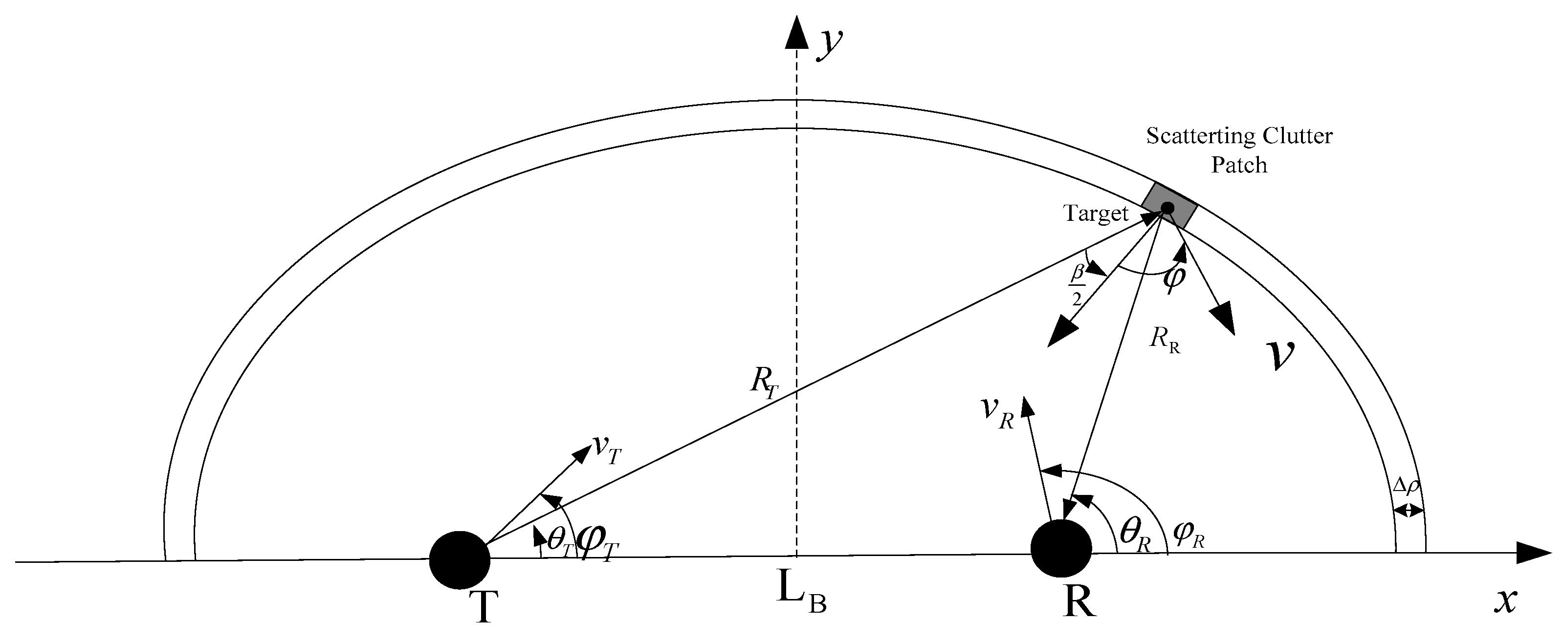
The geometry of the propagation path of a coast–ship bistatic HFSWR system is shown in Figure 1.
It is known that the Doppler frequency between a scattered signal and the direct signal of a bistatic radar system is proportional to the temporal rate of change of the total path length of the scattered signal [21]. Thus, the Doppler frequency of a moving target at the moving transmitting station and moving receiving station of a bistatic HFSWR system can be calculated as follows:
where is the total range of the target relative to both the transmitting station and the receiving station. For a bistatic HFSWR, , where
and
Then,
It can be seen from Equation (4) that the Doppler frequency of a moving target is the sum of the target motion, transmitter motion, and receiver motion [3], i.e., , where is the Doppler shift caused by the motion of the target itself, and is the Doppler frequency caused by the motion of the shipborne mobile platform, which includes that of the transmitting station and the receiving station.
When only the receiving station is placed on a moving shipborne platform, the Doppler frequency of a moving target in a CTSR bistatic HFSWR can be calculated as follows:
Similarly, the Doppler frequency of a moving target in an STCR bistatic HFSWR can be calculated as follows:
For the first-order sea clutter spectrum of an HFSWR, Gill [6] derived the first-order sea surface scattering cross section of a coast-based bistatic HFSWR:
where is the first-order sea wave vector with magnitude K (, where is a wave number), is the acceleration due to gravity, is the Doppler radian frequency, , is the Dirac delta function, m = ±1 means the Doppler shift of the wave, λ is the radar wavelength, and is the ocean spectrum given as a function of the wave vector. As the function satisfy: [6] , then
Thus Equation (7) can be simplified further into the following form:
Then, the first-order Bragg frequencies can be derived as follows according to the property of the Dirac delta function :
When the motion of the shipborne mobile platform is taken into account, the added Doppler shift caused by platform motion on the first-order Bragg frequency should be the same as that on a moving target. Then, the first-order Bragg frequencies are given as
Thus, the first-order sea surface scattering cross section of CTSR and STCR bistatic HFSWR systems can be expressed as
and
where . Accordingly, their first-order Bragg frequencies are given as follows:
It should be noted that the motion of the shipborne platform mentioned here refers primarily to forward navigation movement. When the sway of the ship platform caused by sea waves and wind is considered [7,12], the periodic motion of the shipborne platform can affect the first-order sea clutter spectrum and the target echoes. In addition, surface currents can lead to Doppler shift of the sea clutter spectrum. However, it is inappropriate to use only a single velocity of surface current for different sea areas with different directions of arrival. Therefore, the effects of surface currents were not considered in the model proposed.
3. Simulation Analysis of the First-Order Sea Clutter Spectrum for a Coast–Ship Bistatic HFSWR
As can be seen from the above, the Doppler shift of both the first-order sea clutter spectrum and the moving target echo were affected by the radar frequency, bistatic angle, and velocity of the shipborne platform. To quantitatively analyze the characteristics of the broadening of the sea clutter spectrum and the related blind area, simulation analysis of the first-order sea clutter spectrum for a coast–ship bistatic HFSWR was studied under conditions of different frequencies, different platform velocities, and different elliptical rates. In the following simulation, it was assumed that heading of the shipborne platform was consistent with the navigation direction.
It must be highlighted that the focus of this paper was on the application of bistatic radar target monitoring. For this reason, the Doppler shift of the first-order sea clutter spectrum and the related influence on the blind area are expressed with base units of velocity magnitude (i.e., m) instead of Hz. In addition, as CTSR and STCR are equivalent bistatic configurations when similar antennas and array configurations are used, the simulation results and influence analysis of only the CTSR bistatic radar system are presented here. Simulation results for the STCR bistatic radar system could be obtained by replacing the velocity of the receiving station platform with that of the transmitting station platform.
3.1. Simulation 1: Simulated Space–Time Distribution for Different Headings of the Shipborne Platform
Based on Equation (14), the distribution of the broadening of the first-order sea clutter for a coast–ship bistatic HFSWR when the shipborne platform was anchored is shown in Figure 2. Here, we set the elliptical eccentricity as e = 0.7, frequency as 4.7 MHz, navigation speed = 0 km/h, and wind direction as 90°.
It can be seen from Figure 2 that the broadening ranges of the right sea clutter spectrum and left sea clutter spectrum were symmetrical for a coast–ship bistatic HFSWR when the shipborne platform was anchored, i.e., the width of the right sea clutter spectrum was equal to that of the left sea clutter spectrum when the heading was given. Here, the right first-order spectrum was selected as an example. The right bound retained the value of , while the value of the left bound fRL was
where is the largest bistatic angle for a given elliptical eccentricity , i.e., , and is its corresponding direction of arrival. Here, .
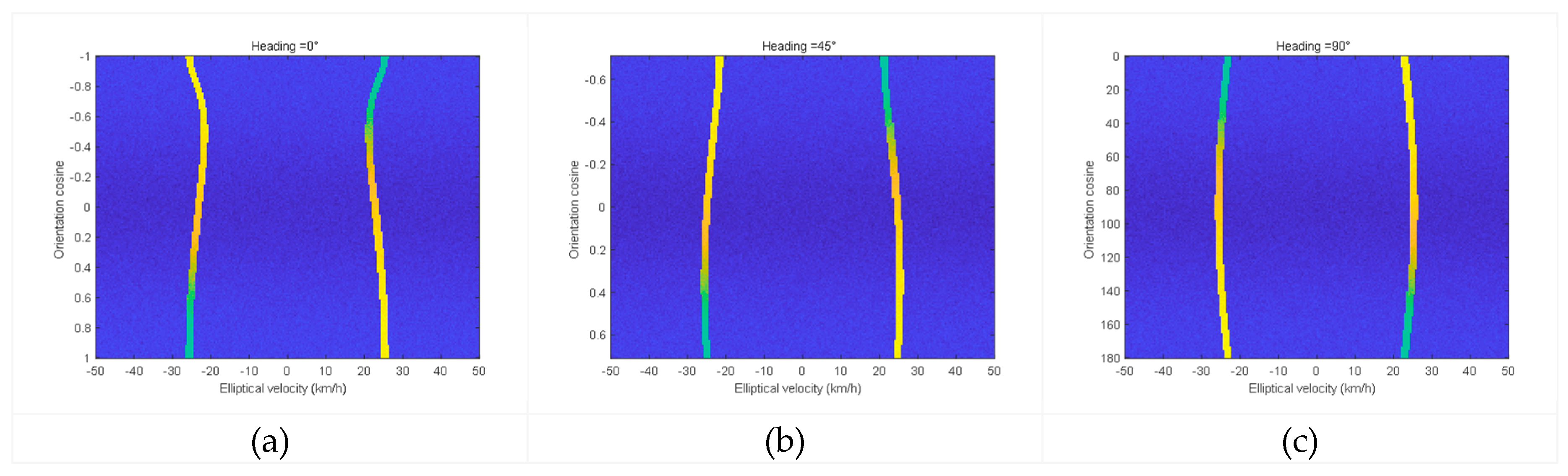
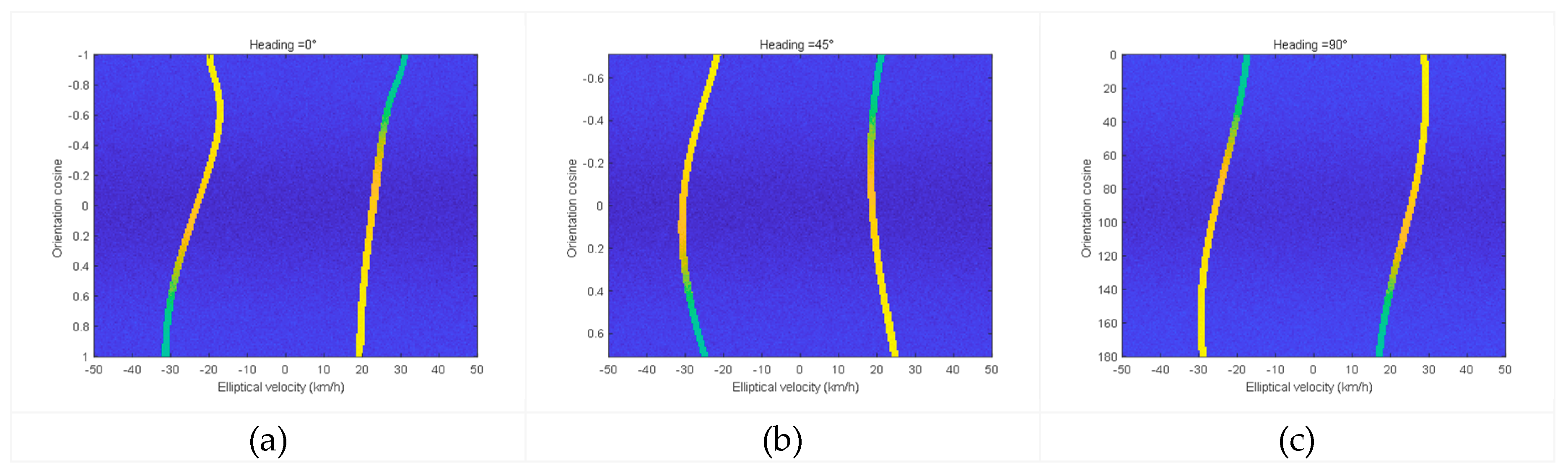
The space–time distribution of the Doppler frequency shift of the first-order sea clutter and the simulation results of the first-order sea clutter spectrum for a CTSR bistatic HFSWR at three different headings when the shipborne platform was anchored are shown in Figure 3. It can be seen that the simulated space–time distribution of the frequency shift of the sea clutter varied with the direction of arrival. The space–time distribution of the Doppler shift of the first-order sea clutter of a coast–ship bistatic HFSWR system is presented as two nonlinear curves with the cosmic value of the incoming direction, and the two curves are symmetrical along the y-axis.
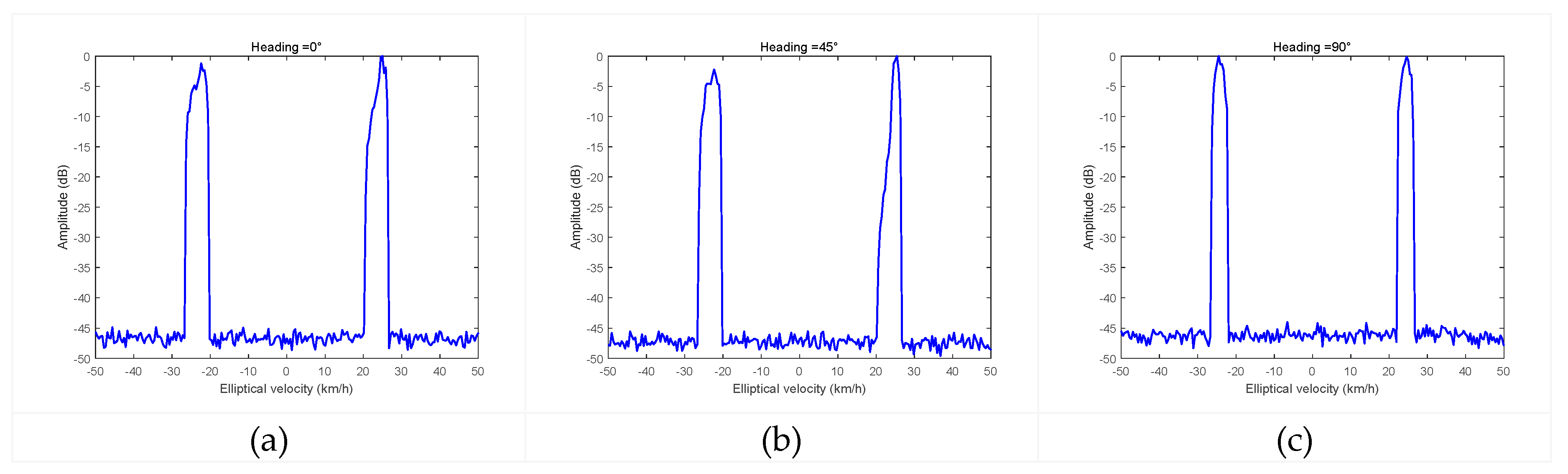
Based on the two-dimensional space–time distribution plots presented in Figure 3, simulation results of the first-order sea clutter spectrum of a coast–ship bistatic HFSWR with different headings on a single channel can be obtained, as shown in Figure 4.
It can be seen from Figure 4 that the broadening ranges of the right first-order sea clutter spectrum and left first-order sea clutter spectrum were symmetrical. As , and , the widths of both the right sea clutter spectrum and the left sea clutter spectrum at the headings of 0° and 45° were equal. The minimum value of the width of the sea clutter spectrum was obtained when . In addition, owing to the change of heading, the angle of the wind direction relative to the principal axis of the receiving array was equivalent to that change, which induced the amplitude variation of the sea clutter spectrum.
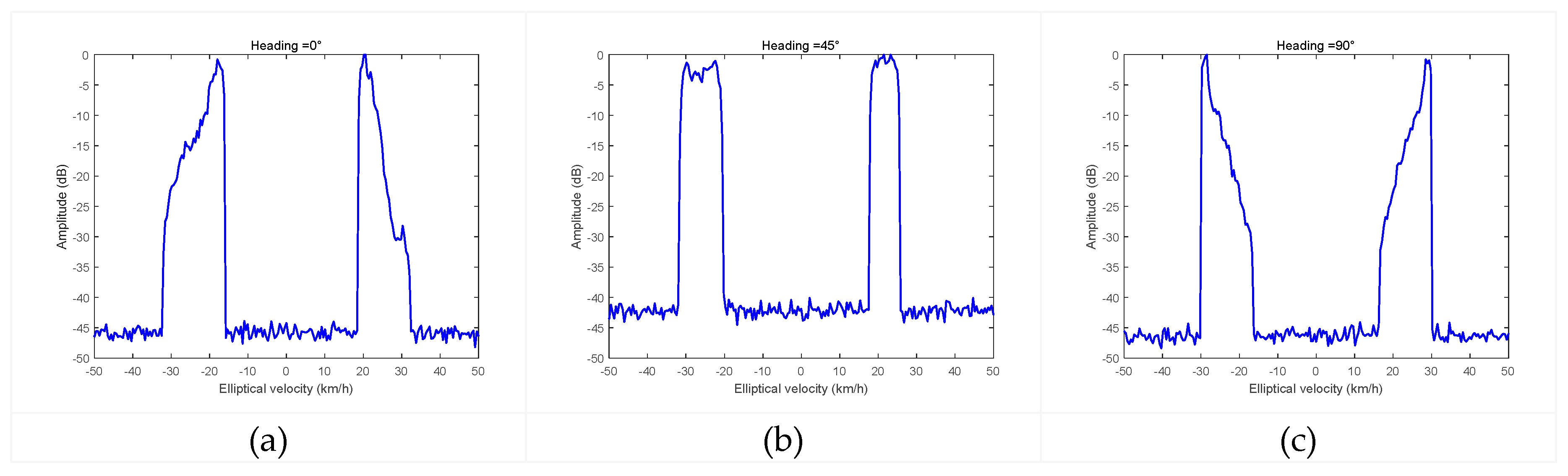
The space–time distribution of the Doppler frequency shift of the first-order sea clutter and the simulation results of the first-order sea clutter spectrum for a CTSR bistatic HFSWR at three different headings when the shipborne platform was navigating with velocity of 11.5 km/h are shown in Figure 5 and Figure 6, respectively. In those cases, the broadening ranges of the right first-order sea clutter spectrum and left first-order sea clutter spectrum were asymmetrical and their widths were not equal.
3.2. Simulation 2: Simulated Space–Time Distribution for Different Shipborne Platform Velocities
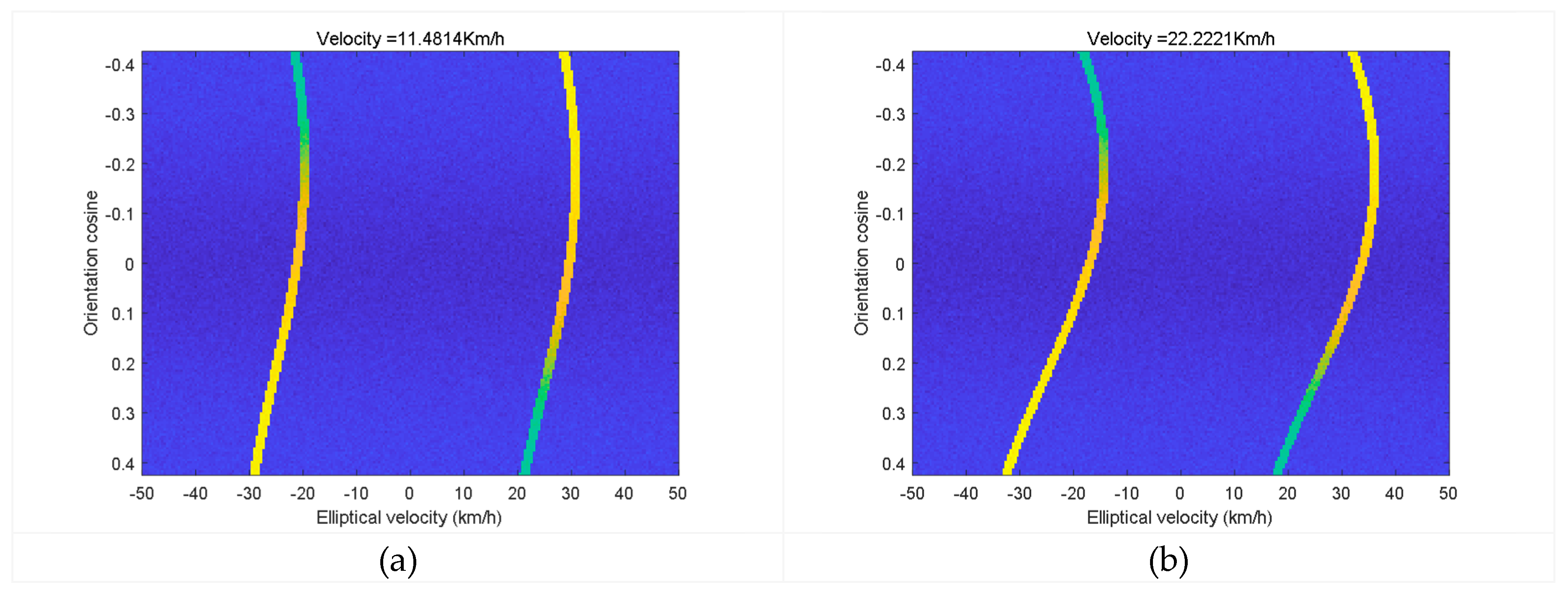
The space–time distribution of the Doppler frequency shift of the first-order sea clutter and the simulation results of the first-order sea clutter spectrum for a CTSR bistatic HFSWR at different velocities are shown in Figure 7 and Figure 8, respectively. Here, we set the elliptical eccentricity as e = 0.22, frequency as 4.7 MHz, heading = 115°, and wind direction as 90°. Simulation results of a monostatic shipborne HFSWR with the same operating conditions are presented for comparative analysis in Figure 8.
It can be seen from Figure 8a that the range of broadening of the first-order sea clutter spectrum of a coast–ship bistatic HFSWR increased when the platform velocity increased, meaning that the range of the blind area caused by first-order sea clutter was widened, which had a greater effect on moving targets falling within these velocity ranges. This is very disadvantageous to target detection. Conversely, with the increase of platform velocity, the echo amplitude of the first-order sea clutter decreased gradually, which led to a higher signal-to-clutter ratio. This is more conducive to the detection and highlighting of moving targets falling into and becoming submerged in the blind area caused by first-order sea clutter.
As can be seen from Figure 8b, the range of broadening of the first-order sea clutter spectrum for a monostatic shipborne HFSWR was obviously larger than that of the coast–ship bistatic HFSWR under the same platform velocity, and even the left and right sea clutter spectra were almost superimposed when the velocity was greater than 24 km/h. For a CTSR bistatic HFSWR, only the receiving station was on the moving platform, while both the transmitting and the receiving stations were on the moving platform in a monostatic shipborne HFSWR system. Therefore, the Doppler shift of the first-order sea clutter spectrum and the related blind area of a coast–ship CTSR bistatic HFSWR were smaller than those of a monostatic shipborne HFSWR.
3.3. Simulation 3: Simulated Space–Time Distribution for Different Radar Frequencies
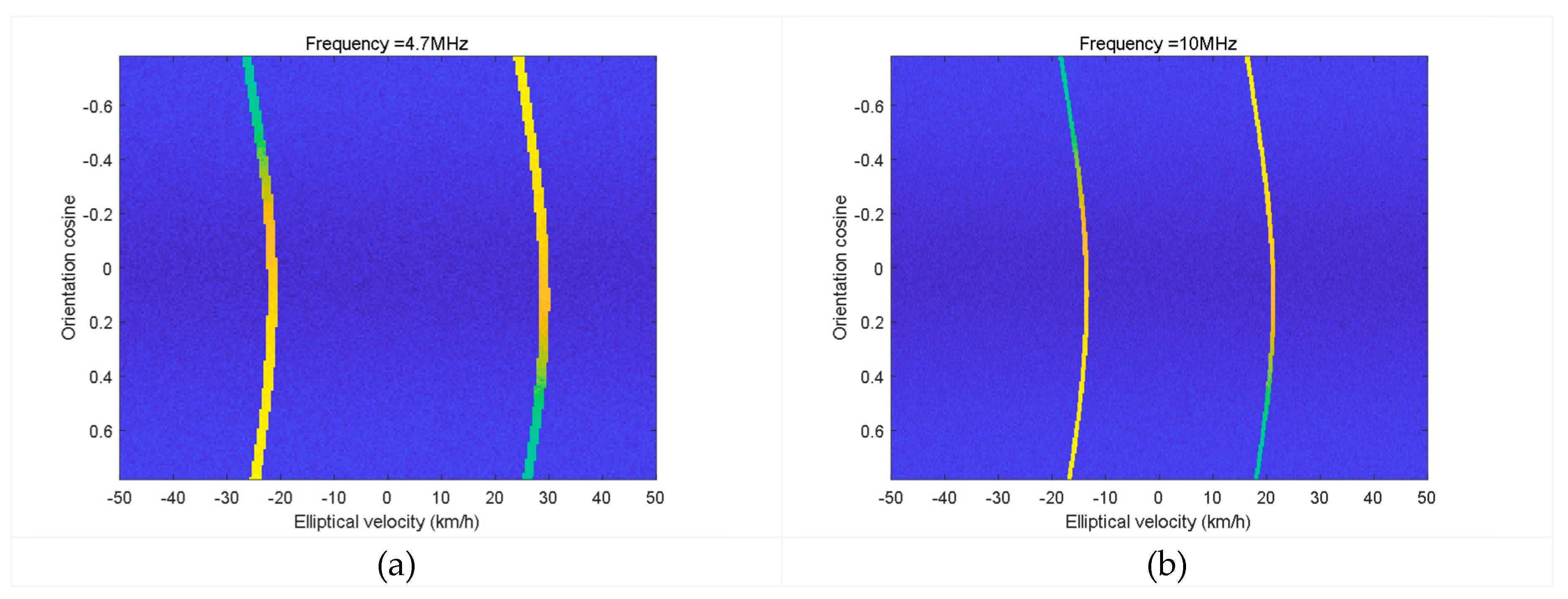
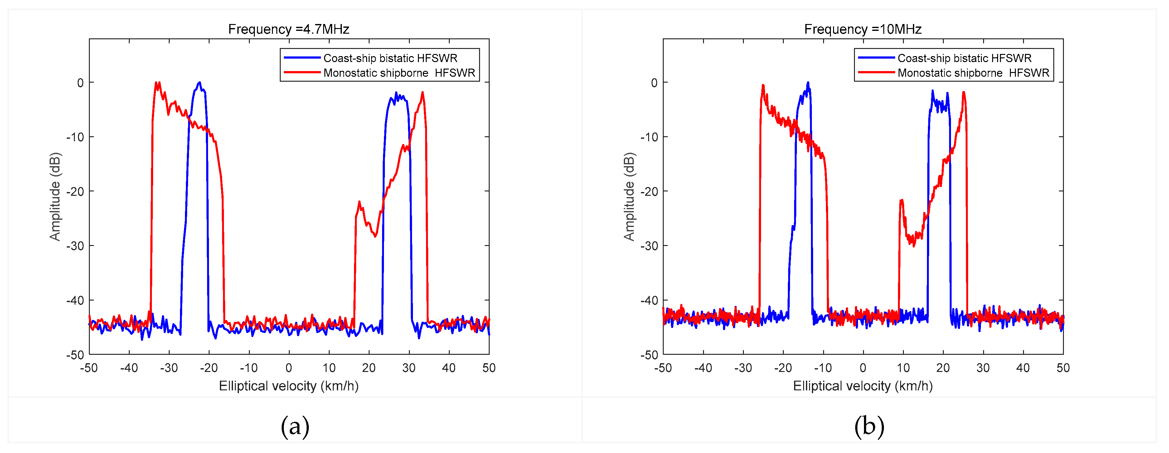
The space–time distribution of the Doppler frequency shift of the first-order sea clutter and the simulation results of the first-order sea clutter spectrum for a CTSR bistatic HFSWR at different frequencies are shown in Figure 9 and Figure 10, respectively. Here, we set the elliptical eccentricity as e = 0.134, shipborne platform velocity = 8 km/h (approximately 4.3 knots), heading °, and wind direction as 90°.
It can be seen from Figure 10 that the widths of the sea clutter blind area of a monostatic shipborne HFSWR at different frequencies but with a constant platform velocity were similar, while their central positions differed. Conversely, both the range of broadening of the first-order sea clutter spectrum and the width of the sea clutter blind area of a coast–ship bistatic HFSWR changed with radar frequency.
3.4. Simulation 4: Simulated Sea Clutter Spectrum for Different Wind Directions
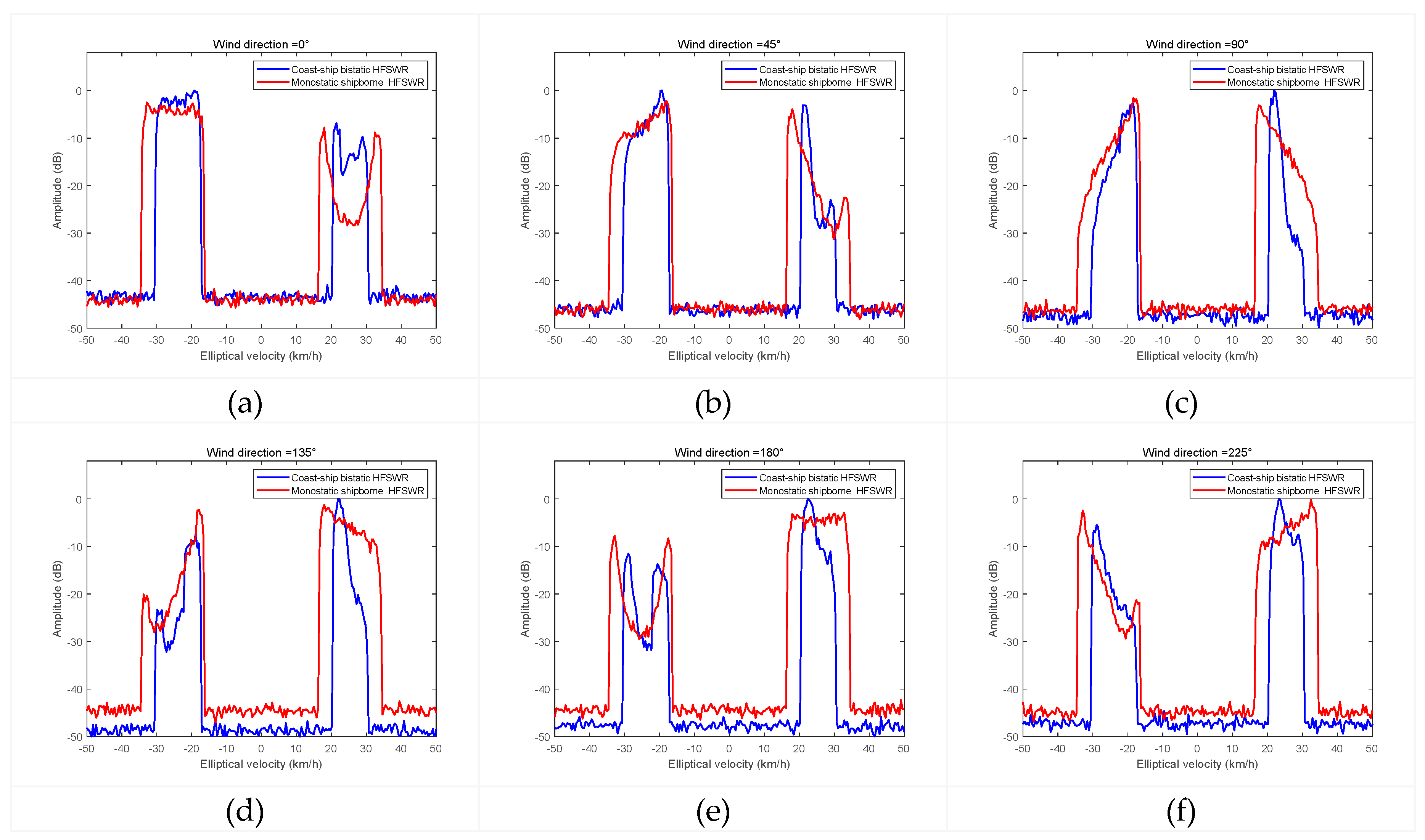
The simulation results of the first-order sea clutter spectrum at wind directions of 0°, 45°, 90°, 135°, 180°, and 225° are shown in Figure 11a–f. Here, we set the elliptical eccentricity as = 0.7, frequency as 4.7 MHz, shipborne platform velocity = 8 km/h, and heading .
It can be seen from Figure 11 that the range of broadening of the first-order sea clutter spectrum of a coast–ship bistatic HFSWR remained unchanged under different wind conditions. Moreover, the width of the first-order sea clutter of the coast–ship bistatic HFSWR was always less than that of the monostatic shipborne HFSWR under the same platform velocity and radar configuration. However, the comparative relationship between the amplitude of the left first-order spectrum and right first-order spectrum was changed, and the related blind area had a different influence on target detection.
Under the condition of 180° wind direction, the average amplitude of the right first-order spectrum relative to the underlying noise was 38 dB, while the average amplitude of the left first-order spectrum was 21 dB, i.e., a difference of 17 dB. Thus, for a moving target with amplitude of 30 dB, if its elliptical velocity were within the right first-order spectrum, it would be submerged completely by sea clutter. However, it could be detected easily if its elliptical velocity were within the left first-order spectrum. For the wind condition of 135°, the situation was the reverse of the 45° condition.
3.5. Simulation 5: Simulated Space–Time Distribution for Different Elliptical Eccentricity
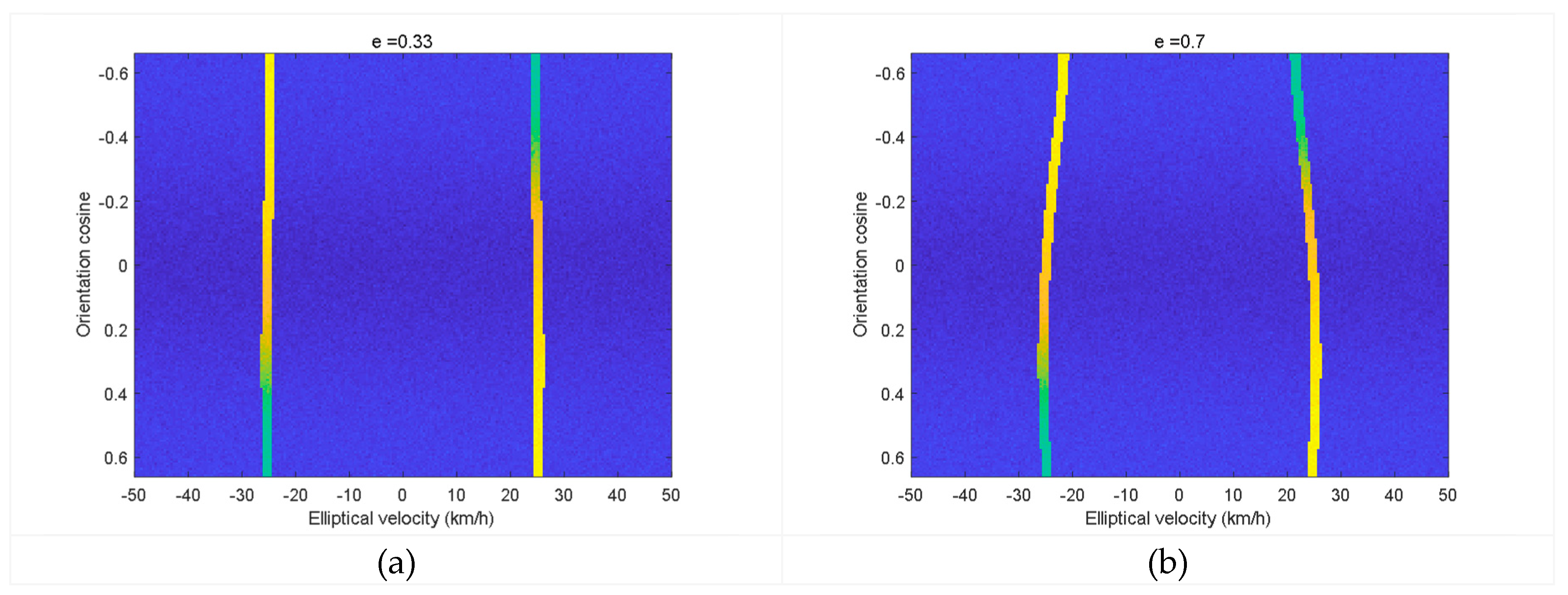
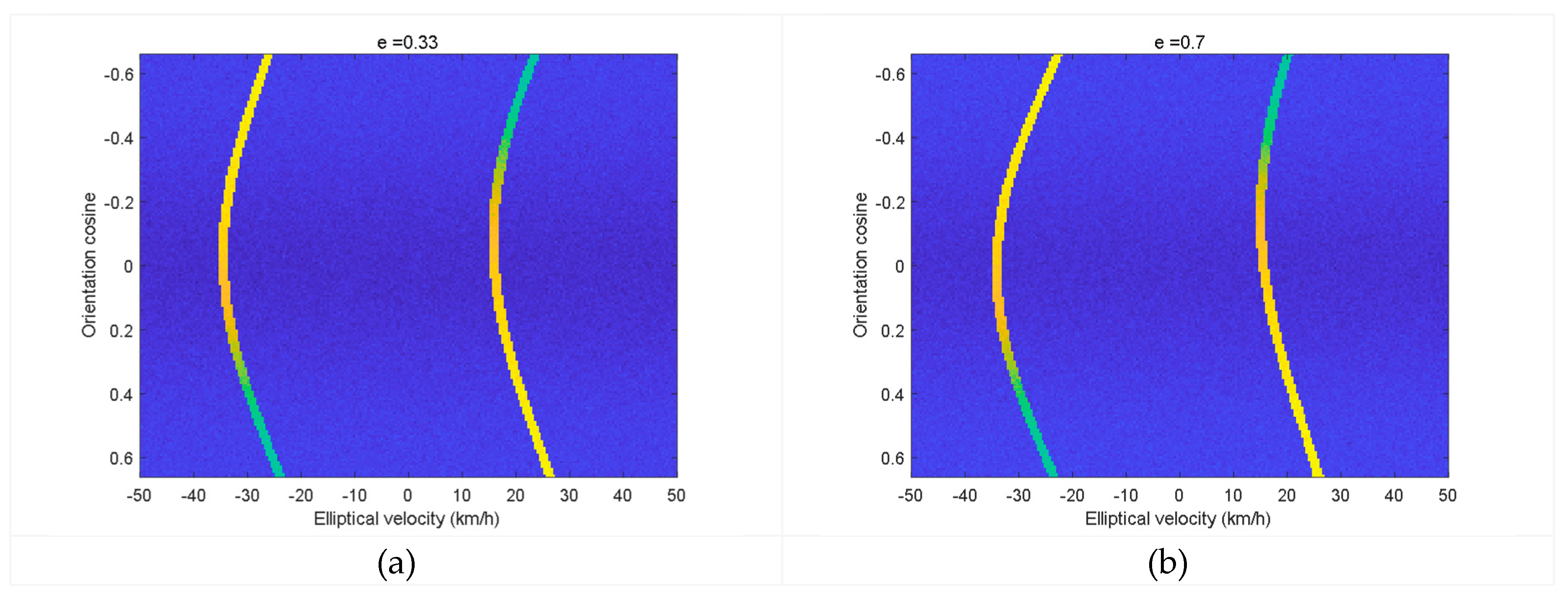
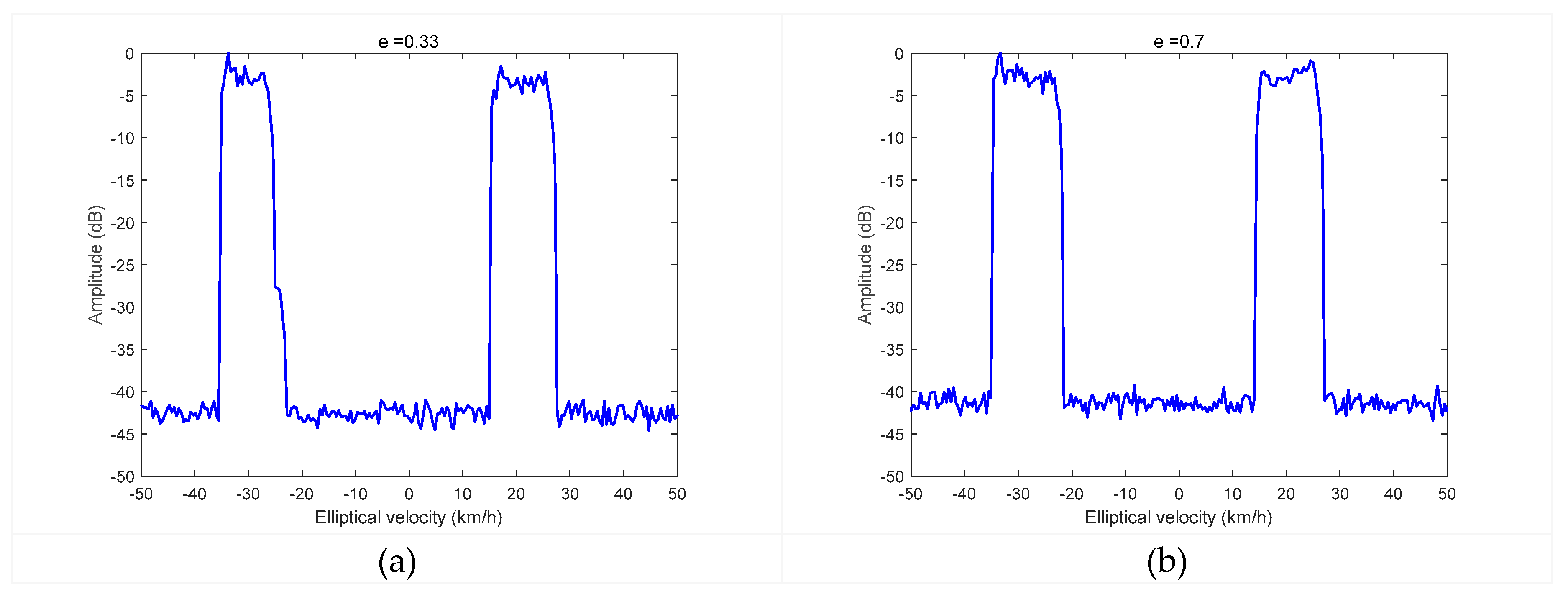
The space–time distribution of the Doppler frequency shift of the first-order sea clutter and the simulation results of the first-order sea clutter spectrum for a CTSR bistatic HFSWR at different elliptical eccentricity are shown in Figure 12, Figure 13, Figure 14 and Figure 15, respectively. Here, we set the frequency as 4.7 MHz, heading = 48.9°, wind direction as 90°, and velocity = 18.5 km/h (approximately 10 knots) when ship was navigating.
As can be seen from Figure 12, Figure 13, Figure 14 and Figure 15, the first-order sea clutter spectrum of e = 0.7 was wider than that of e = 0.33 when the heading = 48.9° in the anchored case, whereas the width of the sea clutter was largely unchanged under different elliptical eccentricity when the ship was navigating with the velocity of 18.5 km/h.
Based on analysis of simulations of the first-order sea clutter spectrum of a coast–ship bistatic HFSWR in navigational state, the range of the detection blind area caused by broadening of the first-order sea clutter spectrum and its influence on target detection can be understood and overcome. The findings could be used to develop appropriate strategies for actual target detection, such as adopting the most suitable navigational speed and heading. For a CTSR bistatic HFSWR system, the principal axis angle of the receiving array and the Doppler frequency shift of the detected target can be changed by adjusting the heading of the platform without changing the platform position. In this way, a moving target signal submerged within each area of sea clutter could be separated from the range of the blind area or adjusted to the side of the sea clutter blind area with less influence. It should be noted that such strategies do not apply to STCR bistatic HFSWR systems.
4. Vessel Target Monitoring Experiment with Coast–Ship Bistatic HFSWR
4.1. Introduction of the Coast–Ship Bistatic HFSWR
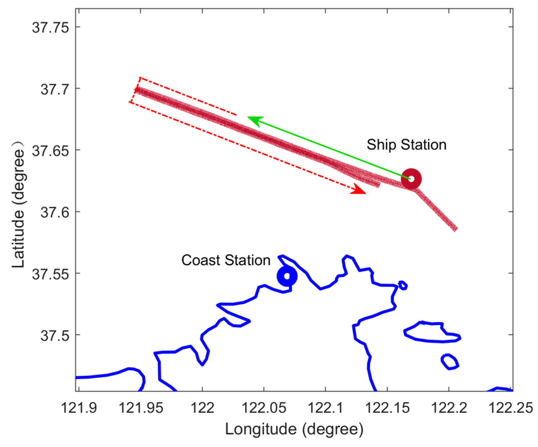
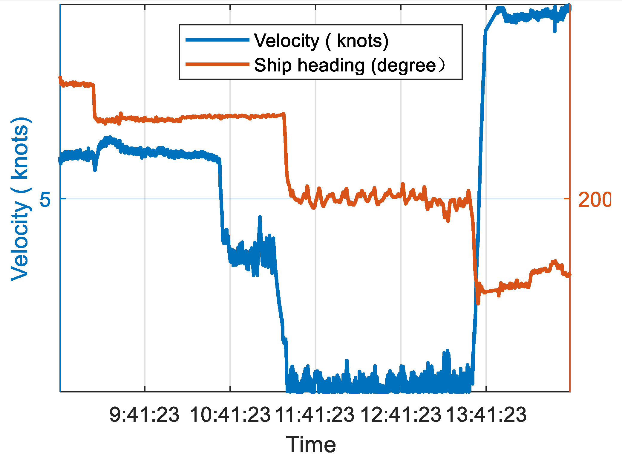
A coast–ship HFSWR experiment was conducted in July 2019 using two Compact Over-horizon Radar for Marine Surveillance HFSWR systems (CORMS). One radar was located on the coast near the city of Weihai (Shandong Province, China; Figure 16), and the other was deployed on the M/V Shun Chang 28. The experimental area comprised the open-water area off the coast near Weihai. The experiment was divided into two periods. The first period, from 09:18:00 to 10:07:00 local time, is indicated by the green line in Figure 16. During this period, measured experimental data using the CTSR bistatic HFSWR system were obtained. The second period, from 10:50:00 to 14:40:00 local time, is indicated by the red dashed line in Figure 16. During this period, measured experimental data using the STCR bistatic HFSWR system were acquired. The velocity and heading of the shipborne platform during the experiment are shown in Figure 17. Here, the heading is given clockwise relative to north.
The CORMS HFSWR system used in the experiment had a solid-state transmitter with maximum peak power of 500 W. The output power of the transmitter could be adjusted continuously. A linear frequency-modulated interrupting continuous wave signal was used, and a double-whip transmitter antenna at the height of 11 m transmitted an omnidirectional pattern. The HF radar receiver was fully digitalized with eight channels, although only five channels were used in the experiment. Each element of the receiving array was a small magnetic cylindrical antenna (length: 0.5 m, diameter: 0.4 m), suitable for shipborne platforms. The radar frequency was 4.7 MHz and the bandwidth was 60 KHz.
In the coast–ship bistatic HFSWR experiment, synchronous transmitter–receiver monostatic HFSWR data were also obtained using a system collocated with the transmitter station. The transmitters and receivers of both radar systems, as well as the two radars, were synchronized using GPS. Both the shore-based receiving array and the shipborne receiving array were composed of five elements but with different element spacing. Owing to the limitation that the length of the shipborne platform was only 88 m, the available array aperture of the shipborne receiving array was only 62 m and its antenna spacing was 15.5 m. Conversely, the antenna spacing of the shore-based receiving array was 29 m, and the array aperture was 116 m, i.e., >100 m. Besides, motion attitude information of the shipborne platform was recorded synchronously using the shipborne inertial navigation system. The measured radar echo spectrum data of the coast–ship bistatic HFSWR system obtained in the experiment are discussed in the following section.
4.2. Interpretation of Experiment Results
Time period 1: CTSR bistatic HFSWR experimental data analysis
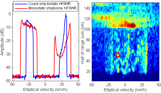
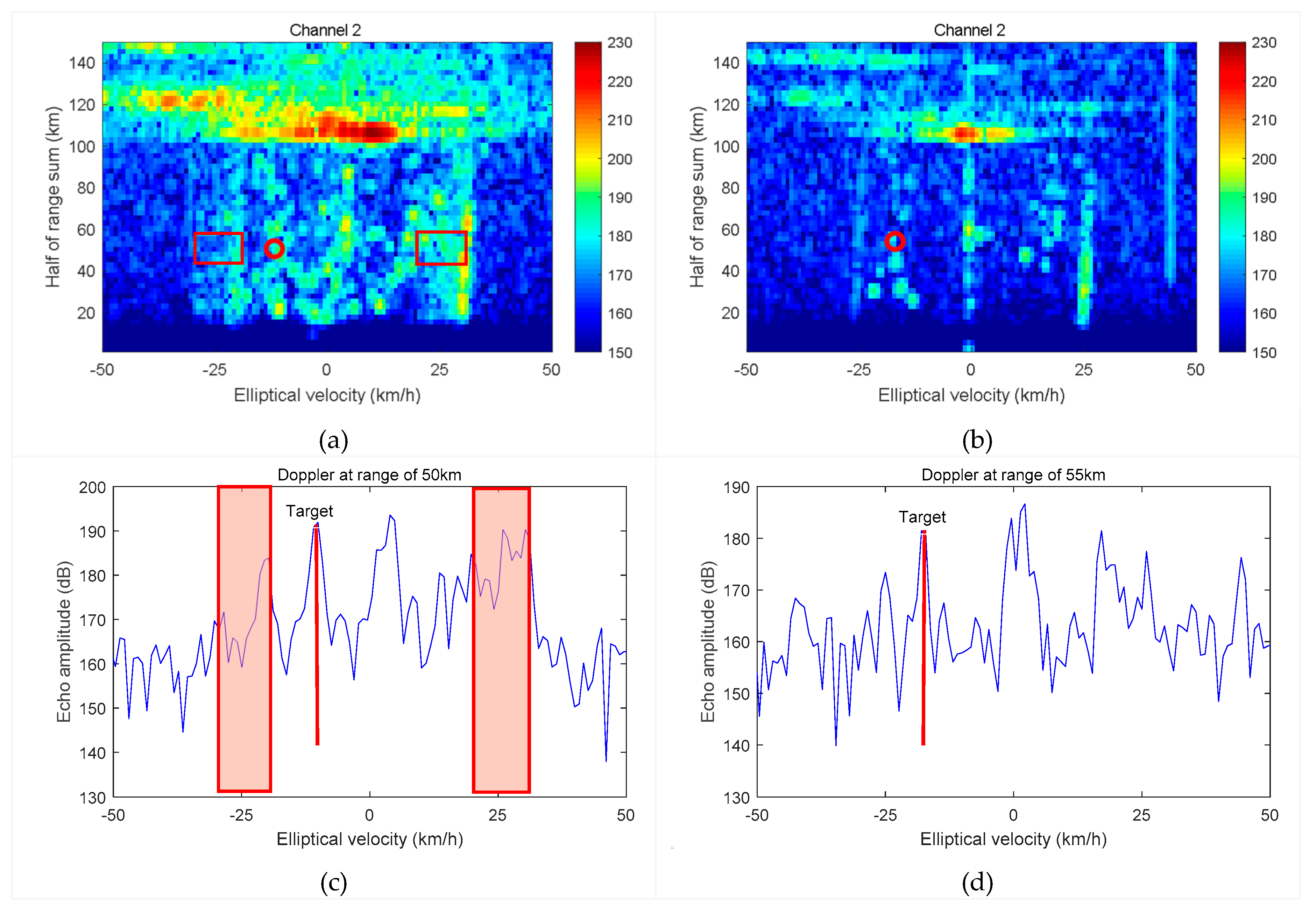
A typical two-dimensional range-Doppler (RD) spectrum of the CTSR bistatic HFSWR and that of the coast-based monostatic HFSWR at a specific time is shown in Figure 18a,b, respectively. At the sample time, the baseline distance between the transmitting station and the receiving station was 12.8 km. The shipborne platform was sailing in a straight line with velocity of 11.48 km/h (6.2 knots), the ship heading was 115° (relative to the baseline), and the main axis angle of the shipborne radar receiving station was 205° (relative to the baseline). The broadening range of the simulated sea clutter spectrum with the same parameter configuration as in the experiment is superimposed on the measured radar spectrum, and it is marked with a red box.
As can be seen from Figure 18, in comparison with the non-broadened first-order sea clutter spectrum of the coast-based monostatic HFSWR, both the left and right first-order sea clutter RD spectra of the CTSR bistatic HFSWR were broadened at the platform velocity 11.48 km/h (6.2 knots), and the broadening of the right first-order sea clutter spectrum was more obvious than that of the left. The width of the right first-order sea clutter was approximately 11.1 km/h (20.8 to 31.9 km/h), and that of the left first-order sea clutter was 10.3 km/h (−18.5 to −28.8 km/h). According to the simulation results (Figure 8a) discussed in Section 3, the theoretical width of the right first-order sea clutter should be 11.3 km/h (20.2 to 31.5 km/h), and that of the left first-order sea clutter should be 10.5 km/h (−18.9 to −29.4 km/h). It can be seen that the measured width values of both the left and the right first-order sea clutter are consistent with their theoretical values. The small deviation of approximately 0.6 km/h (0.17 m/s) of the location of the sea clutter spectrum might have been caused by the existence of ocean currents. In addition, it can be discerned from Figure 18a that the bending characteristics of the first-order Doppler spectrum caused by the bistatic angle were not obvious. This is mainly attributable to two reasons. The first is that the baseline was small relative to the detection distance. The second is that the shipborne receiving station could only receive on the right side of the ship, limiting the detection range of the radar to a certain extent. Both of these factors could lead to smaller eccentricity and a smaller bistatic angle, resulting in the determined bending characteristics of the first-order sea clutter spectrum.
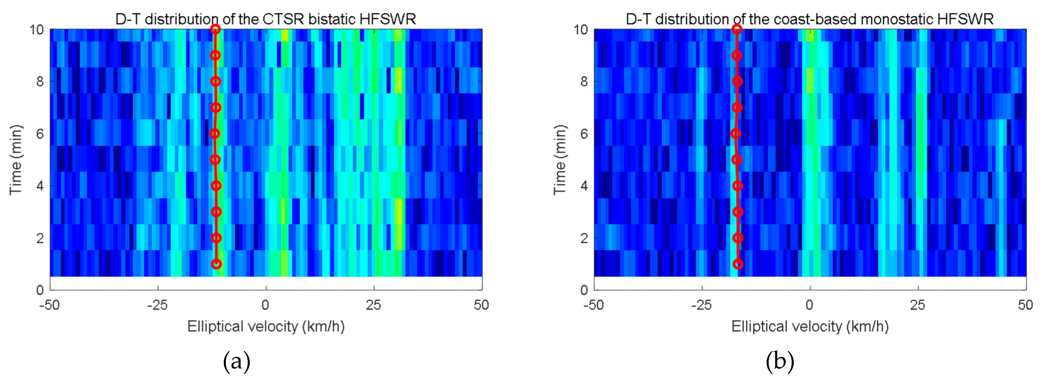
Compared with the broadened first-order sea clutter spectrum, the echo of a moving target (Maritime Mobile Service Identity No: 413551440) was detected simultaneously by the bistatic HFSWR and the coast-based monostatic HFSWR systems. The positions of the target in the two-dimensional RD spectra and in the one-dimensional Doppler spectra are marked with red circles and straight lines, respectively. Its velocity and heading were 19.96 km/h and 289.4° relative to the north, respectively, i.e., , = −167.8529°,, relative to the baseline, and . Based on Equation (5), the theoretical radial velocity was −11.7516 km/h. Its echo appeared in the 20th range unit, i.e., the 74th Doppler unit of the RD spectrum of the CTSR bistatic HFSWR with a signal-to-noise ratio (SNR) value of approximately 30 dB, which means that the half of its range sum was 50.73 km, and the projected elliptical velocity was −11.8127 km/h. It can be seen that the measured velocity of the target is consistent with the theoretical value (−11.7516 km/h). The target’s range relative to the monostatic HFSWR was 54.2269 km and the radial velocity was −17.0557 km/h, with an SNR value of approximately 25 dB. The Doppler-time (D-T) distributions over a 10-min period, onto which the elliptical velocity results were projected using Automatic-Identification-System (AIS) real information were superimposed, are shown in Figure 19. It can be seen that the track of the moving target can be detected clearly, and that the Doppler shift of the target echo within the 10-min period is consistent with the AIS track results.
Time period 2: STCR bistatic HFSWR experimental data analysis
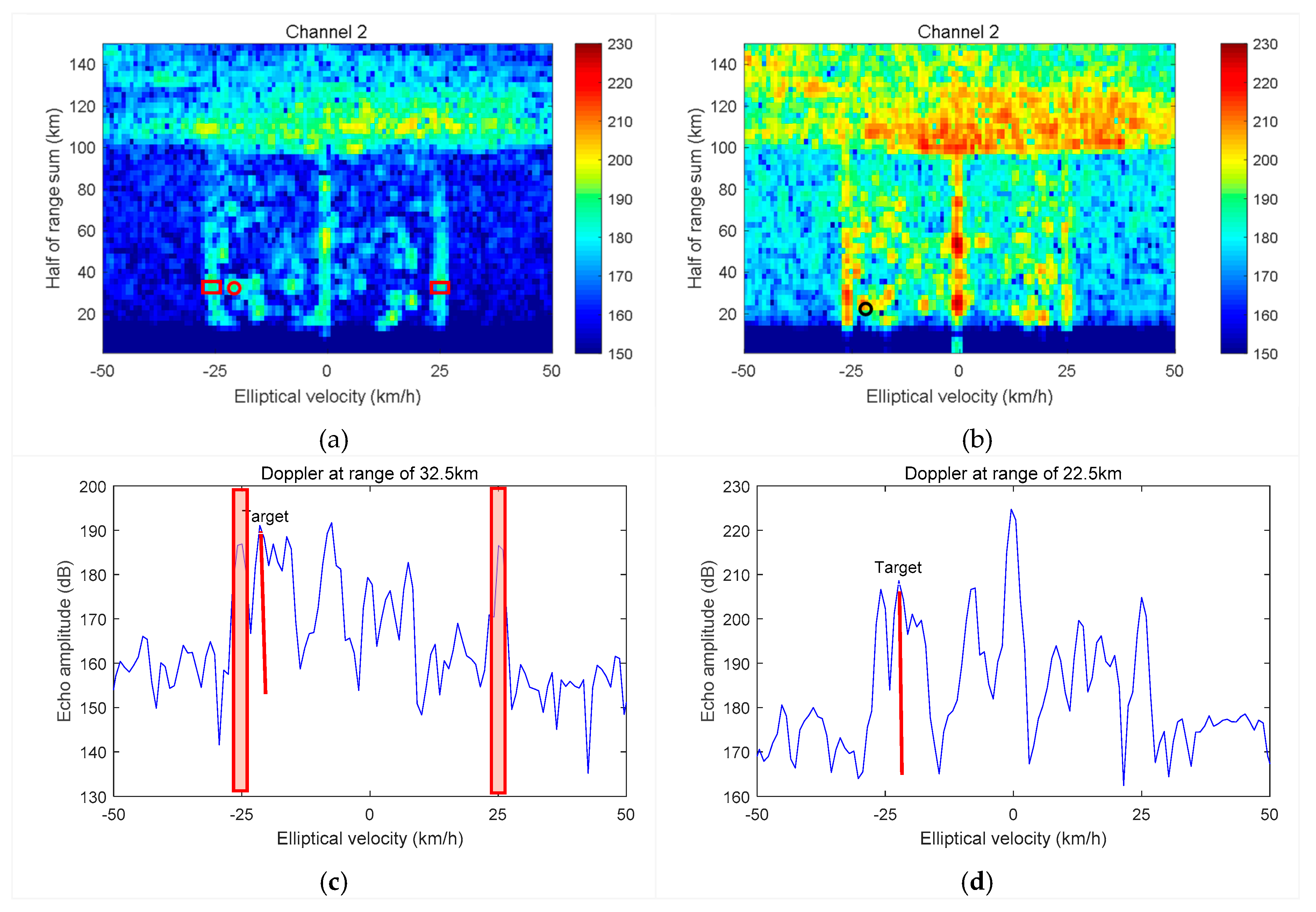
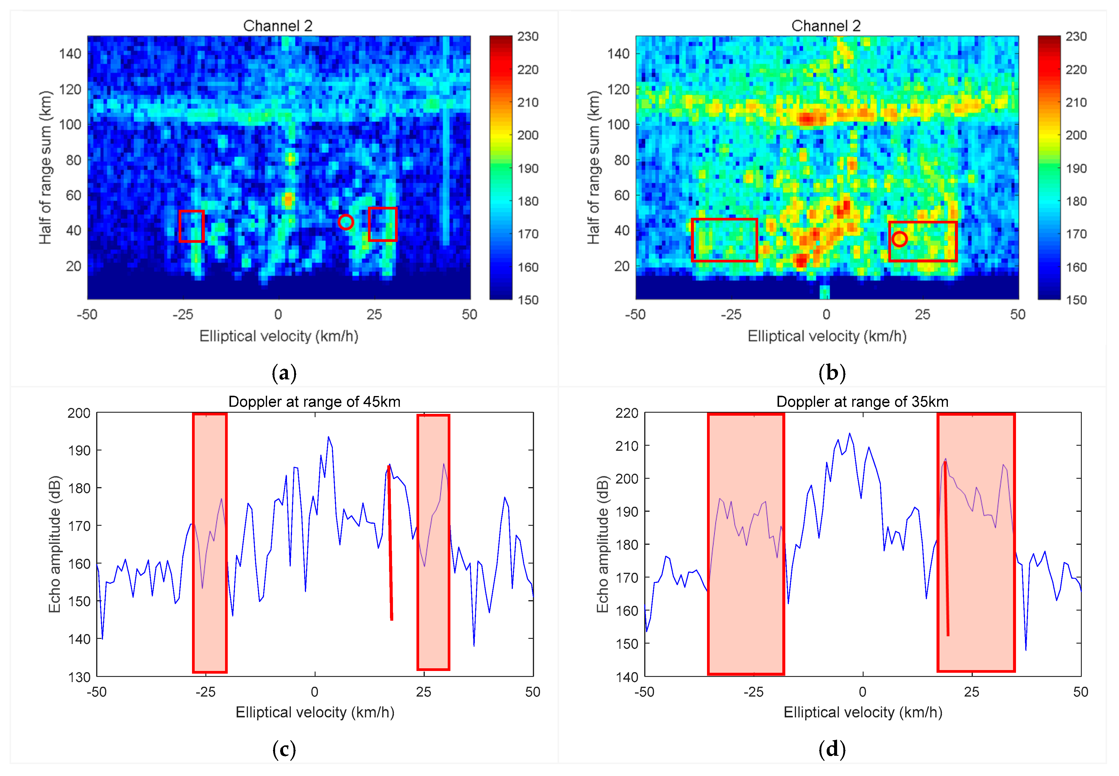
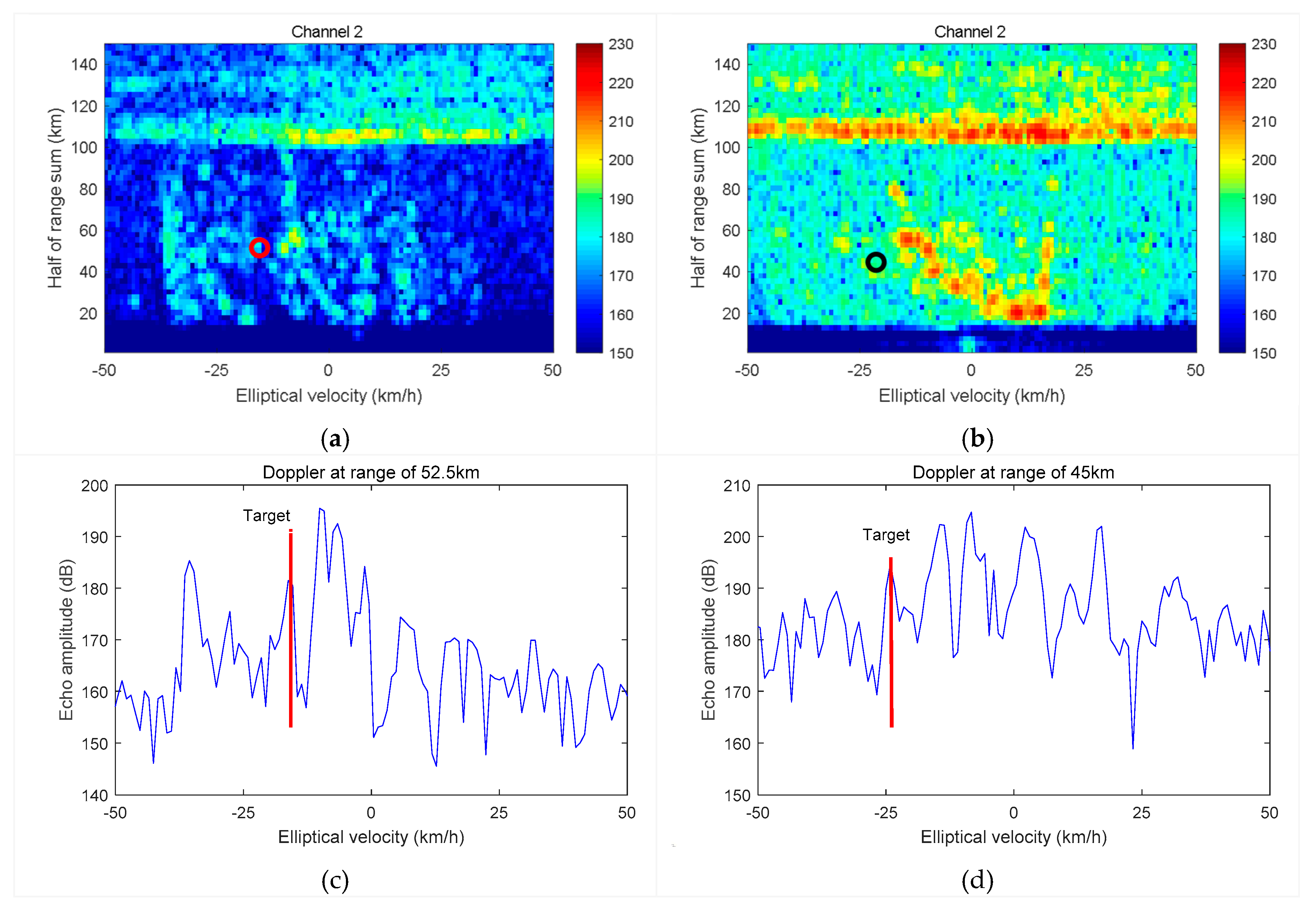
Measured data of the STCR bistatic HFSRW system with different platform speeds were obtained in the second period. The STCR bistatic HFSWR spectrum and the synchronous shipborne monostatic HFSWR data at the velocity of 0 km/h, 7.96 km/h (4.3 knots), and 18.5 km/h (10.0 knots) are shown in Figure 20, Figure 21 and Figure 22, respectively. The heading at the three moments was 54°, 141°, and 115°, respectively (relative to the baseline). For the receiving station, the angle of the main axis was fixed at 310°.
As can be seen from Figure 20, Figure 21 and Figure 22, the bending characteristics of the first-order Doppler spectrum caused by the bistatic angle can be observed, although they are not obvious. When the platform was anchored, the velocity of the platform was zero (Figure 20). In this case, the radar can be regarded as having a fixed transmitting station and a fixed receiving station. Therefore, the first-order sea clutter of the STCR bistatic HFSWR was not broadened, which was the same outcome as that of the shipborne monostatic HFSWR. The target echo in the RD spectrum of each of the two radar systems was very clear.
When the platform velocity was approximately 4.3 knots, the broadening of the first-order sea clutter in the RD spectrum (Figure 21) of the bistatic HFSWR was not obvious and most targets were easily detected. The width of the left first-order sea clutter was 6.2 km/h (−20.6 to −26.8 km/h), and that of the right first-order sea clutter was 6.1 km/h (24.1 to 30.2 km/h). According to the simulation results (Figure 10a in Section 3), under the same conditions, the theoretical width of the left first-order sea clutter should be 6.1 km/h (−20.6 to −26.7 km/h), and that of the right first-order sea clutter should be 6.5 km/h (23.7 to 30.2 km/h). Thus, the broadening range of the measured sea clutter spectrum is consistent with the theoretical value. In Figure 22c, the SNR value of the target of concern was approximately 17 dB for the STCR bistatic HFSWR. In contrast, the first-order sea clutter in the RD spectrum of the monostatic HFSWR was obviously broadened. Although the range of the first-order spectrum was wide, the obvious outer boundary can be seen coupled with the influence of land clutter, i.e., the moving target marked in the figure can still be detected, but the signal-to-clutter ratio was reduced to approximately 10 dB.
When the platform velocity reached 10 knots (Figure 22), the scene was very different from the previous two examples. For the STCR bistatic HFSWR, as the coast-based receiving station was obscured by surrounding land, the received signal came only from a limited range of the incoming direction. Therefore, the range of broadening of the left first-order sea clutter spectrum and the Doppler shift of the land clutter were obviously smaller than the theoretical values. For the shipborne monostatic HFSWR, as the shipborne platform was on the way back, the main axis angle of the radar receiving station was 205°, and the detection range of the shipborne receiving station was mainly facing land. Consequently, there was no obvious boundary to be found because of the wide range of the first-order sea clutter. However, the presence of land clutter was obvious, varying continuously with range and velocity in the radar echo.
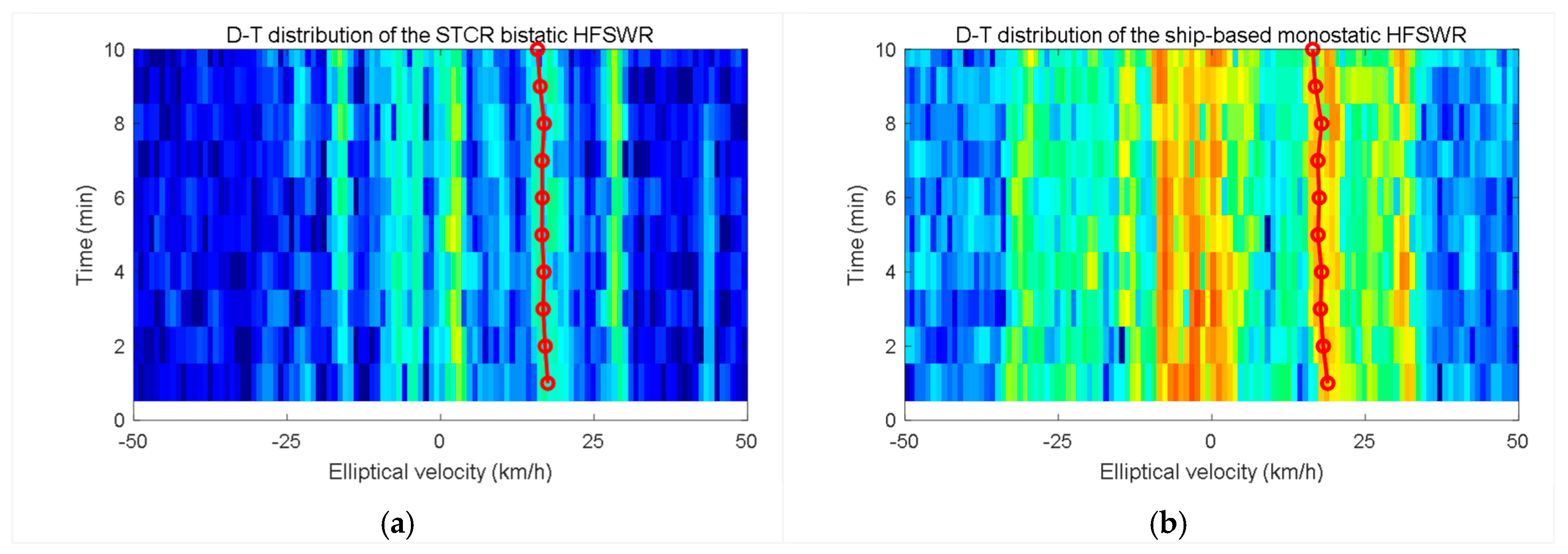
Similar to the above, Figure 23 shows the D-T distributions and AIS results of the STCR bistatic HFSWR and ship-based monostatic HFSWR at the platform velocity of 4.3 knots (). At this time, , ,. The moving target () was detected at the range of 44.75 km with an elliptical velocity of approximately 17.46 km/h by the STCR bistatic HFSWR based on Equation (6), whereas it was detected at the range of 35 km with a radial velocity of approximately 18.87 km/h by the ship-based monostatic HFSWR. The Doppler shift of the target echo in the measured radar data is largely consistent with the AIS track results.
5. Conclusions
By combining the advantages of coast-based bistatic HFSWR and shipborne monostatic HFSWR, a coast–ship bistatic HFSWR system has potential in anti-electronic interference and expanded detection range by fully exploiting the advantage of the flexibility of a shipborne platform. To investigate the characteristics of the first-order sea clutter spectrum, and the related blind area and its influence on target detection, the theoretical formulas for a coast–ship bistatic HFSWR system were derived. Moreover, simulations of the first-order sea clutter spectrum under different radar parameters and different shipborne platform velocities were analyzed. From the simulation results and its influence on target detection, it can be concluded that the Doppler shift of both the first-order sea clutter and the moving target were affected mainly by the velocity of the moving platform and the bistatic angle in a coast–ship bistatic HFSWR. Broadening of the first-order sea clutter spectrum will cause a blind area for target detection. When the shipborne platform was anchored, the broadening ranges of the right sea clutter spectrum and left sea clutter spectrum were symmetrical, and the widths of the right sea clutter and left sea clutter were equal. When the shipborne platform was navigating, the broadening ranges of the first-order sea clutter spectrum on the left and right were asymmetrical, and their widths were not equal, owing to the combined influence of the bistatic angle and the platform motion. In addition, the broadening range of the first-order sea clutter spectrum of a coast–ship bistatic HFSWR increased with the increase of platform velocity in most cases. At the same platform velocity, both the broadening range of the first-order sea clutter spectrum and the width of the sea clutter blind area of a coast–ship bistatic HFSWR changed with radar frequency, and the width of the first-order sea clutter of a coast–ship bistatic HFSWR was less than that of a shipborne monostatic HFSWR. Under the condition of higher platform velocity, although the detection blind area caused by sea clutter was wider, the echo amplitude of sea clutter was lower, and the lower SNR was beneficial for target detection. Although the comparative relationship between the amplitude of the left first-order spectrum and the right first-order spectrum changed under different wind conditions, the range of broadening of the first-order sea clutter spectrum remained unchanged. The analysis of measured experimental data revealed that the broadening range of the first-order sea clutter and of the frequency shift of a moving target are consistent with theoretical and simulation results. The findings of this study further the understanding of the theoretical formulas and measured spectrum data of the two types of coast-ship bistatic HFSWR.
It should be noted that under the condition of a moving platform, irrespective of whether a monostatic shipborne HFSWR or a coast–ship bistatic HFSWR is used, the first-order sea clutter will be broadened markedly in the channel spectrum. In general, beam data rather than channel data are used in target detection to obtain a better SNR. Therefore, the influence of sea clutter broadening within the beam data of coast–ship bistatic HFSWR should be considered in the process of motion compensation or sea clutter suppression for target detection, and related research will be undertaken in the future.
Author Contributions
Conceptualization, Y.J.; methodology, Y.J. and C.Y. (Chao Yue); validation, W.G., and H.S.; formal analysis, J.L.; investigation, Y.W., C.Y. (Chao Yue) and W.G.; resources, Y.J. and C.Y. (Changjun Yu); Data Curation: W.G. and J.L.; writing—original draft preparation, Y.J.; writing—review and editing, Y.W. and M.L.; visualization, H.S.; supervision, J.Z. and M.L; project administration, Y.J.; funding acquisition, Y.J. All authors have read and agreed to the published version of the manuscript.
Funding
This research was funded by the National Key R & D Program of China (grant number 2017YFC1405202); and the National Natural Science Foundation of China (grant number 61671166).
Acknowledgments
The authors thank the anonymous reviewers for their comments and suggestions that have helped to improve the quality and the readability of this article. We thank James Buxton MSc from Liwen Bianji, Edanz Group China (www.liwenbianji.cn./ac), for editing the English text of this manuscript.
Conflicts of Interest
The authors declare no conflict of interest.
References
- Ponsford, A.M. Surveillance of the 200 Nautical Mile Exclusive Economic Zone (EEZ) Using High Frequency Surface Wave Radar (HFSWR). Can. J. Remote Sens. 2001, 27, 354–360. [Google Scholar] [CrossRef]
- Liu, Y.T.; Xu, R.Q.; Zhang, N. Progress in HFSWR research at Harbin Institute of Technology. In Proceedings of the International Conference on Radar, Adelaide, Australia, 3–5 September 2003; pp. 522–528. [Google Scholar]
- Nicholas, J. Bistatic Radar, 2nd ed.; SciTech Publishing Inc.: Troy, NY, USA, 2005; pp. 119–123. [Google Scholar]
- Yao, G.W.; Xie, J.H.; Huang, W.M. Ocean Surface Cross Section for Bistatic HF Radar Incorporating a Six DOF Oscillation Motion Model. Remote Sens. 2019, 11, 2738. [Google Scholar] [CrossRef] [Green Version]
- Huang, W.M.; Gill, E.; Wu, X.B.; Li, L. Measurement of Sea Surface Wind Direction Using Bistatic High-Frequency Radar. IEEE Trans. Geosci. Remote Sens. 2012, 50, 4117–4122. [Google Scholar] [CrossRef]
- Gill, E.W. The Scattering of High Frequency Electromagnetic Radiation from the Ocean Surface: An Analysis Based on a Bistatic Ground Wave Radar Configuration. Ph.D. Thesis, Memorial University of Newfoundland, St. John’s, NL, Canada, January 1999. [Google Scholar]
- Gill, E.W.; Walsh, J. High-frequency bistatic cross sections of the ocean surface. Radio Sci. 2001, 36, 1459–1475. [Google Scholar] [CrossRef]
- Barrick, D.E. First-order Theory and Analysis of MF/HF/VHF Scatter from the Sea. IEEE Trans. Antennas Propag. 1972, 20, 2–10. [Google Scholar] [CrossRef] [Green Version]
- Lipa, B.J.; Barrick, D.E. Extraction of sea state from HF radar sea echo: Mathematical theory and modeling. Radio Sci. 1986, 21, 81–100. [Google Scholar] [CrossRef]
- Xie, J.; Sun, M.; Ji, Z. Space-time Model of the First-Order Sea Clutter in Onshore Bistatic High Frequency Surface Wave Radar. IET Radar Sonar Navig. 2015, 9, 55–61. [Google Scholar] [CrossRef]
- Walsh, J.; Huang, W.; Gill, E.W. The First-Order High Frequency Radar Ocean Surface Cross Section for an Antenna on a Floating Platform. IEEE Trans. Antennas Propag. 2010, 58, 2994–3003. [Google Scholar] [CrossRef]
- Walsh, J.; Huang, W.; Gill, E.W. The second-order high frequency radar ocean surface cross section for an antenna on a floating platform. IEEE Trans. Antennas Propag. 2012, 60, 4804–4813. [Google Scholar] [CrossRef]
- Khoury, J.; Guinvarch, R.; Gillard, R. Sea-echo Doppler spectrum perturbation of the received signals from a floating high-frequency surface wave radar. IET Radar Sonar Navig. 2012, 6, 165–171. [Google Scholar] [CrossRef]
- Xie, J.; Yuan, Y.; Liu, Y.T. Experimental analysis of sea clutter in shipborne HFSWR. IEE Proc. Radar Sonar Navig. 2001, 148, 67–71. [Google Scholar] [CrossRef]
- Xie, J.; Sun, M.; Ji, Z. First-order ocean surface cross-section for shipborne HFSWR. Electron. Lett. 2013, 49, 1005–1026. [Google Scholar] [CrossRef]
- Li, F.L.; Chen, B.X.; Zhang, S.H. Design of Multi-carrier Digital Frequency Synthesizer for Coast-ship Multi-static GroundWave OTH Radar. In Proceedings of the 2006 CIE International Conference on Radar, Shanghai, China, 6–19 October 2006; pp. 1–5. [Google Scholar]
- Chen, B.X.; Chen, D.F.; Zhang, S.H. Experimental system and experimental results for coast-ship bi/multistatic ground-wave over-the-horizon radar. In Proceedings of the 2006 CIE International Conference on Radar, Shanghai, China, 6–19 October 2006; pp. 36–40. [Google Scholar]
- Chen, B.X.; Chen, D.F. Estimation of Gain and Phase Perturbations for Transmit Array Based on Parameter Transfer in Coast-Ship Bistatic SWOTHR. Acta Electron. Sin. 2011, 39, 2184–2189. [Google Scholar]
- Liu, C.B.; Chen, B.X.; Chen, D.F. Analysis of First-order Sea Clutter in a Shipborne Bistatic High Frequency Surface Wave Radar. In Proceedings of the 2006 CIE International Conference on Radar, Shanghai, China, 6–19 October 2006; pp. 1656–1659. [Google Scholar]
- Zhu, Y.; Wei, Y.; Tong, P. First order sea clutter cross section for bistatic shipborne HFSWR. J. Syst. Eng. Electron. 2017, 28, 681–689. [Google Scholar]
- Skolnik, M.I. An Analysis of Bistatic Radar. Aerosp. Navig. Electron. Ire Trans. 1961, ANE-8, 19–27. [Google Scholar] [CrossRef]
Figure 1.
The two-dimensional coordinate system confined to a bistatic plane formed by transmitter site T and receiver site R. LB is the distance of the baseline range between T and R that is coincident with the x-axis. All angles are described anticlockwise relative to the x-axis. To consider the two types of coast–ship bistatic high-frequency surface wave radar (HFSWR) systems simultaneously, both the transmitting station and the receiving station were set as shipborne platforms. The transmitter and receiver have projected velocity vectors of magnitude and and aspect angles and with respect to the -axis, respectively. For a given moving target, its velocity vector projected onto the bistatic plane has magnitude and aspect angle referenced to the bistatic bisector. The distance from the target to T and R is and , respectively, and and describe the angles of and with respect to the -axis, respectively. The bistatic angle is β, and is the range resolution.

Figure 2.
Distribution of the broadening of the first-order sea clutter of a coast–ship bistatic HFSWR when the shipborne platform was anchored.
Figure 2.
Distribution of the broadening of the first-order sea clutter of a coast–ship bistatic HFSWR when the shipborne platform was anchored.

Figure 3.
Space–time distribution of the Doppler frequency shift of the first-order sea clutter for a coast-transmit ship-receive (CTSR) bistatic HFSWR at different headings when the shipborne platform was anchored: (a) 0°, (b) 45°, and (c) 90°.
Figure 3.
Space–time distribution of the Doppler frequency shift of the first-order sea clutter for a coast-transmit ship-receive (CTSR) bistatic HFSWR at different headings when the shipborne platform was anchored: (a) 0°, (b) 45°, and (c) 90°.

Figure 4.
Simulation results of the first-order sea clutter spectrum for a CTSR bistatic HFSWR at different headings: (a) 0°, (b) 45°, and (c) 90°.
Figure 4.
Simulation results of the first-order sea clutter spectrum for a CTSR bistatic HFSWR at different headings: (a) 0°, (b) 45°, and (c) 90°.

Figure 5.
Space–time distribution of the Doppler frequency shift of the first-order sea clutter for a CTSR bistatic HFSWR at different headings when the shipborne platform was navigating: (a) 0°, (b) 45°, and (c) 90°.
Figure 5.
Space–time distribution of the Doppler frequency shift of the first-order sea clutter for a CTSR bistatic HFSWR at different headings when the shipborne platform was navigating: (a) 0°, (b) 45°, and (c) 90°.

Figure 6.
Simulation results of the first-order sea clutter spectrum for a CTSR bistatic HFSWR navigating at different headings: (a) 0°, (b) 45°, and (c) 90°.
Figure 6.
Simulation results of the first-order sea clutter spectrum for a CTSR bistatic HFSWR navigating at different headings: (a) 0°, (b) 45°, and (c) 90°.

Figure 7.
Space–time distribution of the Doppler frequency shift of the first-order sea clutter for a CTSR bistatic HFSWR at different velocities: (a) = 11.48 km/h (6.2 knots) and (b) = 22.2 km/h (12 knots).
Figure 7.
Space–time distribution of the Doppler frequency shift of the first-order sea clutter for a CTSR bistatic HFSWR at different velocities: (a) = 11.48 km/h (6.2 knots) and (b) = 22.2 km/h (12 knots).

Figure 8.
Simulation results of the first-order sea clutter spectrum for a CTSR bistatic HFSWR at different velocities: (a) = 11.48 km/h (6.2 knots) and (b) = 22.2 km/h (12 knots).
Figure 8.
Simulation results of the first-order sea clutter spectrum for a CTSR bistatic HFSWR at different velocities: (a) = 11.48 km/h (6.2 knots) and (b) = 22.2 km/h (12 knots).

Figure 9.
Space–time distribution of the Doppler frequency shift of the first-order sea clutter for a CTSR bistatic HFSWR at different frequencies: (a) = 4.7 MHz and (b) = 10 MHz.
Figure 9.
Space–time distribution of the Doppler frequency shift of the first-order sea clutter for a CTSR bistatic HFSWR at different frequencies: (a) = 4.7 MHz and (b) = 10 MHz.

Figure 10.
Simulation results of the first-order sea clutter spectrum for a CTSR bistatic HFSWR at different frequencies: (a) = 4.7 MHz and (b) = 10 MHz.
Figure 10.
Simulation results of the first-order sea clutter spectrum for a CTSR bistatic HFSWR at different frequencies: (a) = 4.7 MHz and (b) = 10 MHz.

Figure 11.
Simulation results of the first-order sea clutter spectrum for a CTSR bistatic HFSWR at different wind directions: (a) 0°, (b) 45°, (c) 90°, (d) 135°, (e) 180°, and (f) 225°.
Figure 11.
Simulation results of the first-order sea clutter spectrum for a CTSR bistatic HFSWR at different wind directions: (a) 0°, (b) 45°, (c) 90°, (d) 135°, (e) 180°, and (f) 225°.

Figure 12.
Space–time distribution of the Doppler frequency shift of the first-order sea clutter for a CTSR bistatic HFSWR when the ship was anchored: (a) e = 0.33 and (b) e = 0.7.
Figure 12.
Space–time distribution of the Doppler frequency shift of the first-order sea clutter for a CTSR bistatic HFSWR when the ship was anchored: (a) e = 0.33 and (b) e = 0.7.

Figure 13.
Simulation results of the first-order sea clutter spectrum for a CTSR bistatic HFSWR when the ship was anchored: (a) e = 0.33 and (b) e = 0.7.
Figure 13.
Simulation results of the first-order sea clutter spectrum for a CTSR bistatic HFSWR when the ship was anchored: (a) e = 0.33 and (b) e = 0.7.

Figure 14.
Space–time distribution of the Doppler frequency shift of the first-order sea clutter for a CTSR bistatic HFSWR when the ship was navigating: (a) e = 0.33 and (b) e = 0.7.
Figure 14.
Space–time distribution of the Doppler frequency shift of the first-order sea clutter for a CTSR bistatic HFSWR when the ship was navigating: (a) e = 0.33 and (b) e = 0.7.

Figure 15.
Simulation results of the first-order sea clutter spectrum for a CTSR bistatic HFSWR when the ship was navigating: (a) e = 0.33 and (b) e = 0.7.
Figure 15.
Simulation results of the first-order sea clutter spectrum for a CTSR bistatic HFSWR when the ship was navigating: (a) e = 0.33 and (b) e = 0.7.

Figure 16.
Location of coast-based radar station and navigation route of shipborne platform.

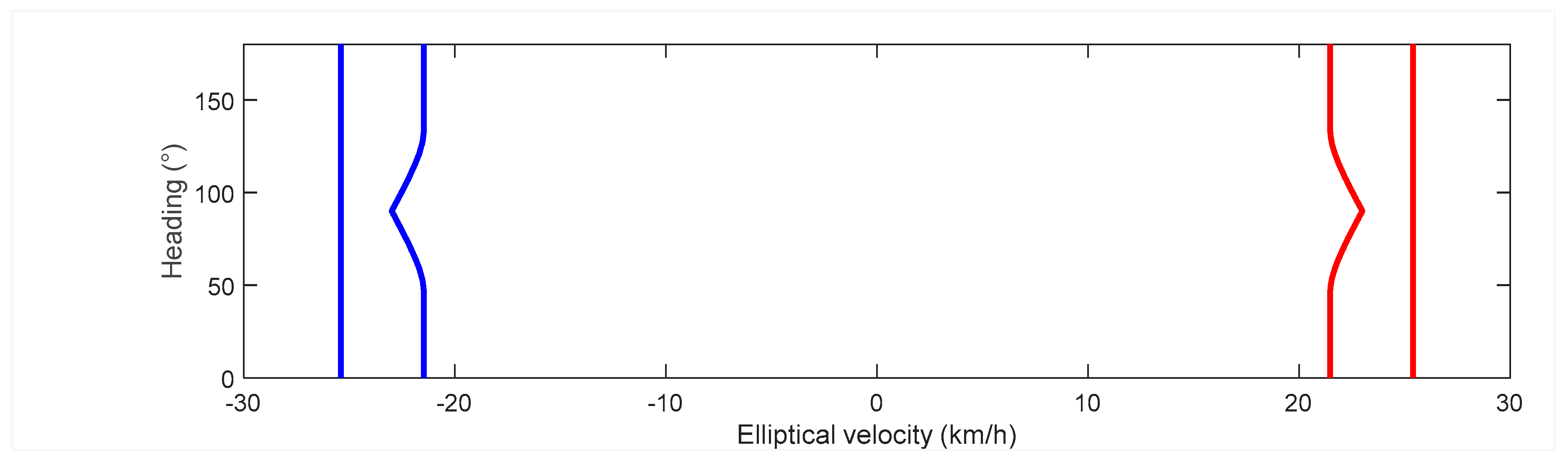
Figure 17.
Velocity and heading of shipborne platform.

Figure 18.
Doppler spectrum of the CTSR bistatic HFSWR and of the coast-based monostatic HFSWR at the velocity of 11.7 km/h (6.2 knots); (a) RD spectrum of the CTSR bistatic HFSWR; (b) RD spectrum of the coast-based monostatic HFSWR; (c) Doppler data of the CTSR bistatic HFSWR at the range of 50 km; (d) Doppler data of the coast-based monostatic HFSWR at the range of 55 km.

Figure 19.
Doppler-time (D-T) distribution and Automatic-Identification-System (AIS) results for the CTST bistatic HFSWR and coast-based monostatic HFSWR; (a) D-T distribution of the CTSR bistatic HFSWR; (b) D-T distribution of the coast-based monostatic HFSWR.
Figure 19.
Doppler-time (D-T) distribution and Automatic-Identification-System (AIS) results for the CTST bistatic HFSWR and coast-based monostatic HFSWR; (a) D-T distribution of the CTSR bistatic HFSWR; (b) D-T distribution of the coast-based monostatic HFSWR.

Figure 20.
Doppler spectra of the STCR bistatic HFSWR and ship-based monostatic HFSWR systems at the velocity of 0 knots. (a) RD spectrum of the STCR bistatic HFSWR; (b) RD spectrum of the ship-based monostatic HFSWR; (c) Doppler spectrum of the STCR bistatic HFSWR at the range of 32.5 km; (d) Doppler spectrum of the ship-based monostatic HFSWR at the range of 22.5 km.

Figure 21.
Doppler spectra of the STCR bistatic HFSWR and ship-based monostatic HFSWR systems at the velocity of approximately 4.3 knots. (a) RD spectrum of the STCR bistatic HFSWR; (b) RD spectrum of the ship-based monostatic HFSWR; (c) Doppler spectrum of the STCR bistatic HFSWR at the range of 45 km; (d) Doppler spectrum of the ship-based monostatic HFSWR at the range of 35 km.

Figure 22.
Doppler spectra of the STCR bistatic HFSWR and ship-based monostatic HFSWR systems at the velocity of approximately 10.0 knots. (a) RD spectrum of the STCR bistatic HFSWR; (b) RD spectrum of the ship-based monostatic HFSWR; (c) Doppler spectrum of the STCR bistatic HFSWR at the range of 52.5 km; (d) Doppler spectrum of the ship-based monostatic HFSWR at the range of 45 km.

Figure 23.
D-T distribution and AIS results for the STCR bistatic HFSWR and ship-based monostatic HFSWR. (a) D-T distribution of the STCR bistatic HFSWR; (b) D-T distribution of the ship-based monostatic HFSWR.
Figure 23.
D-T distribution and AIS results for the STCR bistatic HFSWR and ship-based monostatic HFSWR. (a) D-T distribution of the STCR bistatic HFSWR; (b) D-T distribution of the ship-based monostatic HFSWR.

© 2020 by the authors. Licensee MDPI, Basel, Switzerland. This article is an open access article distributed under the terms and conditions of the Creative Commons Attribution (CC BY) license (http://creativecommons.org/licenses/by/4.0/).
Share and Cite
MDPI and ACS Style
Ji, Y.; Zhang, J.; Wang, Y.; Yue, C.; Gong, W.; Liu, J.; Sun, H.; Yu, C.; Li, M. Coast–Ship Bistatic HF Surface Wave Radar: Simulation Analysis and Experimental Verification. Remote Sens. 2020, 12, 470. https://doi.org/10.3390/rs12030470
AMA Style
Ji Y, Zhang J, Wang Y, Yue C, Gong W, Liu J, Sun H, Yu C, Li M. Coast–Ship Bistatic HF Surface Wave Radar: Simulation Analysis and Experimental Verification. Remote Sensing. 2020; 12(3):470. https://doi.org/10.3390/rs12030470
Chicago/Turabian StyleJi, Yonggang, Jie Zhang, Yiming Wang, Chao Yue, Weichun Gong, Junwei Liu, Hao Sun, Changjun Yu, and Ming Li. 2020. "Coast–Ship Bistatic HF Surface Wave Radar: Simulation Analysis and Experimental Verification" Remote Sensing 12, no. 3: 470. https://doi.org/10.3390/rs12030470
Note that from the first issue of 2016, this journal uses article numbers instead of page numbers. See further details here.