Coastal Turbidity Derived From PROBA-V Global Vegetation Satellite

Abstract

PROBA-V (Project for On-Board Autonomy-Vegetation) is a global vegetation monitoring satellite. The spectral quality of the data and the coverage of PROBA-V over coastal waters provide opportunities to expand its use to other applications. This study tests PROBA-V data for the retrieval of turbidity in the North Sea region. In the first step, clouds were masked and an atmospheric correction, using an adapted version of iCOR, was performed. The resulted water leaving radiance reflectance was validated against AERONET-OC stations, yielding a coefficient of determination of 0.884 in the RED band. Next, turbidity values were retrieved using the RED band. The PROBA-V retrieved turbidity data was compared with turbidity data from CEFAS Smartbuoys and ad-hoc measurement campaigns. This resulted in a coefficient of determination of 0.69. Finally, a time series of 1.5 year of PROBA-V derived turbidity data was plotted over MODIS data to check consistencies in both datasets. Seasonal dynamics were noted with high turbidity in autumn and winter and low values in spring and summer. For low values, PROBA-V and MODIS yielded similar results, but while MODIS seems to saturate around 50 FNU, PROBA-V can reach values up till almost 80 FNU.

1. Introduction

Coastal areas are of high ecological and economic value. However, they are subject to intense human-induced environmental pressures. An effective monitoring system can help in the operational management and safeguarding of the coastal areas. Satellite observations are a valuable asset for coastal managers, as they provide a spatial and temporal context and access to an historic archive. From reflectance observed by satellite sensors, water quality parameters of surface waters can be derived such as turbidity [1,2]. Surface water refers to the upper (centi)meters of the water column. The exact light penetration depth is often unknown and depends on the clarity of the water and wavelength. Ocean Color (OC) sensors are typically used to monitor marine environments. They offer a good compromise between spatial resolution (0.25–1 km) and temporal revisit time (approx. 1 day). A variety of algorithms and methods, with different degree of complexity, have been developed to convert water-leaving radiance reflectance from OC sensors into turbidity. Examples include Moderate Resolution Imaging Spectrometer (MODIS) [3,4,5], Medium Resolution Imaging Spectrometer (MERIS) [6,7] and its recent successor SENTINEL-3 Ocean and Land Color Instrument (OLCI) [8]. However, the spatial or temporal resolution of OC sensors is often not sufficient to monitor near-shore dynamics. As an alternative, non-OC passive optical sensors can be addressed. These sensors were designed for other purposes such as atmosphere or vegetation monitoring. Despite their lower spectral quality (lower Signal-To-Noise Ratio (SNR)), previous studies have shown their added value for turbidity monitoring. Examples of non-OC derived turbidity products include SEVIRI [9], Landsat-8 [10,11,12] and Sentinel-2 [12,13,14].

This study looks into the, for coastal applications unexploited, non-OC Project for On-Board Autonomy-Vegetation (PROBA-V) satellite for turbidity retrieval. PROBA-V, launched in 2013, was designed for global vegetation monitoring: images with a spatial resolution of 300 m are acquired daily, while a global coverage at 100 m spatial resolution is achieved every five days [15]. The multispectral pushbroom spectrometer onboard measures radiance in four broad spectral bands (BLUE, RED, Near Infrared (NIR) and Short-Wave Infrared (SWIR)) and covers a large swatch of 2285 km. Regions up till at least 100 km from the coastline are recorded. Despite the broad spectral bands, the spectral quality of the sensor and the temporal and spatial resolution provides opportunities to include PROBA-V, together with other (non-) OC sensors, in coastal monitoring programs [16]. First, the methodology to derive turbidity maps from PROBA-V data is presented. The intermediate water leaving radiance reflectance data are compared with AERONET-OC data to validate the atmospheric correction procedure over water scenes. Turbidity estimates are compared with CEFAS SmartBuoy measurements and field data. Finally, an intercomparison of the turbidity products between PROBA-V and MODIS AQUA is performed.

2. Materials and Methods

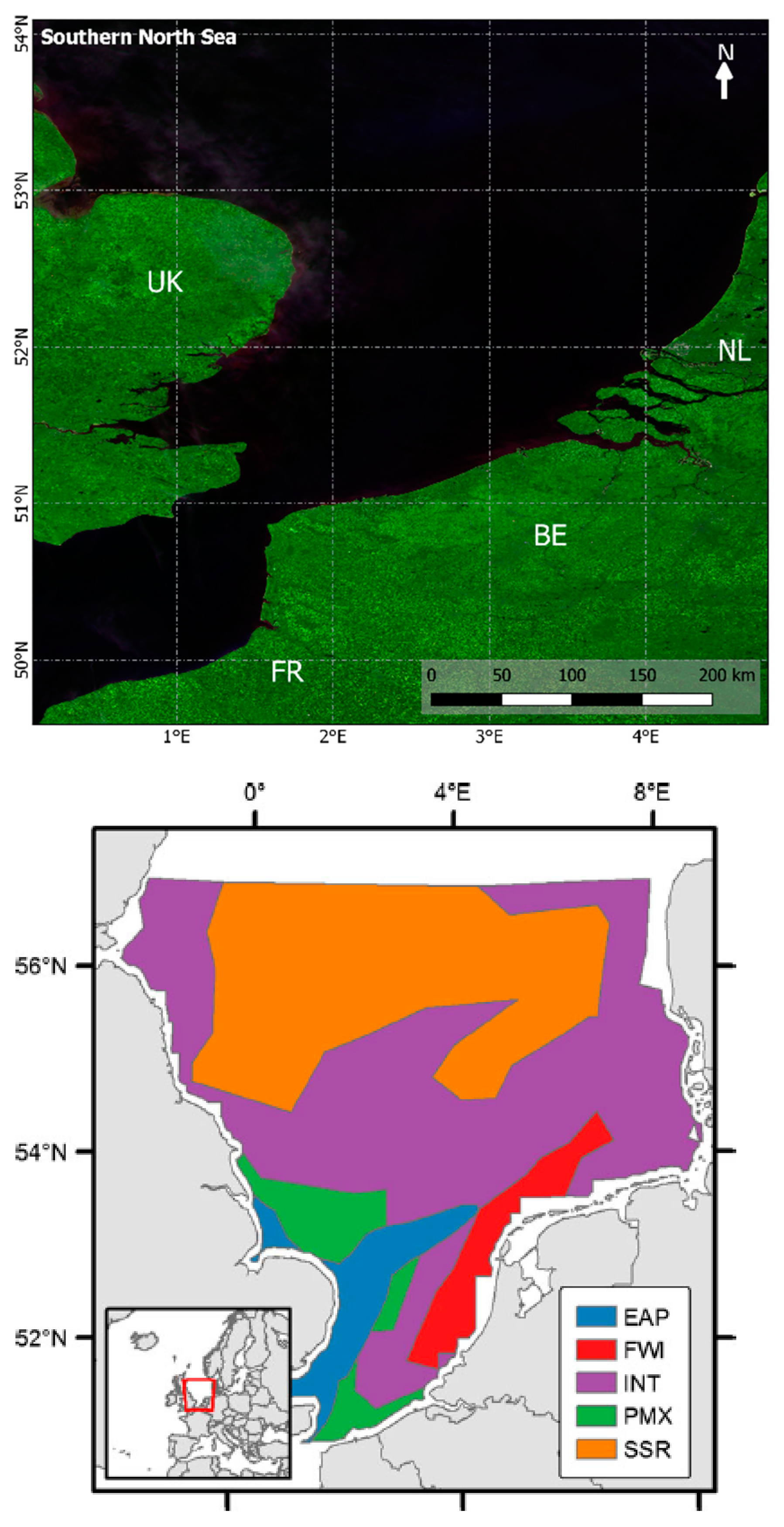
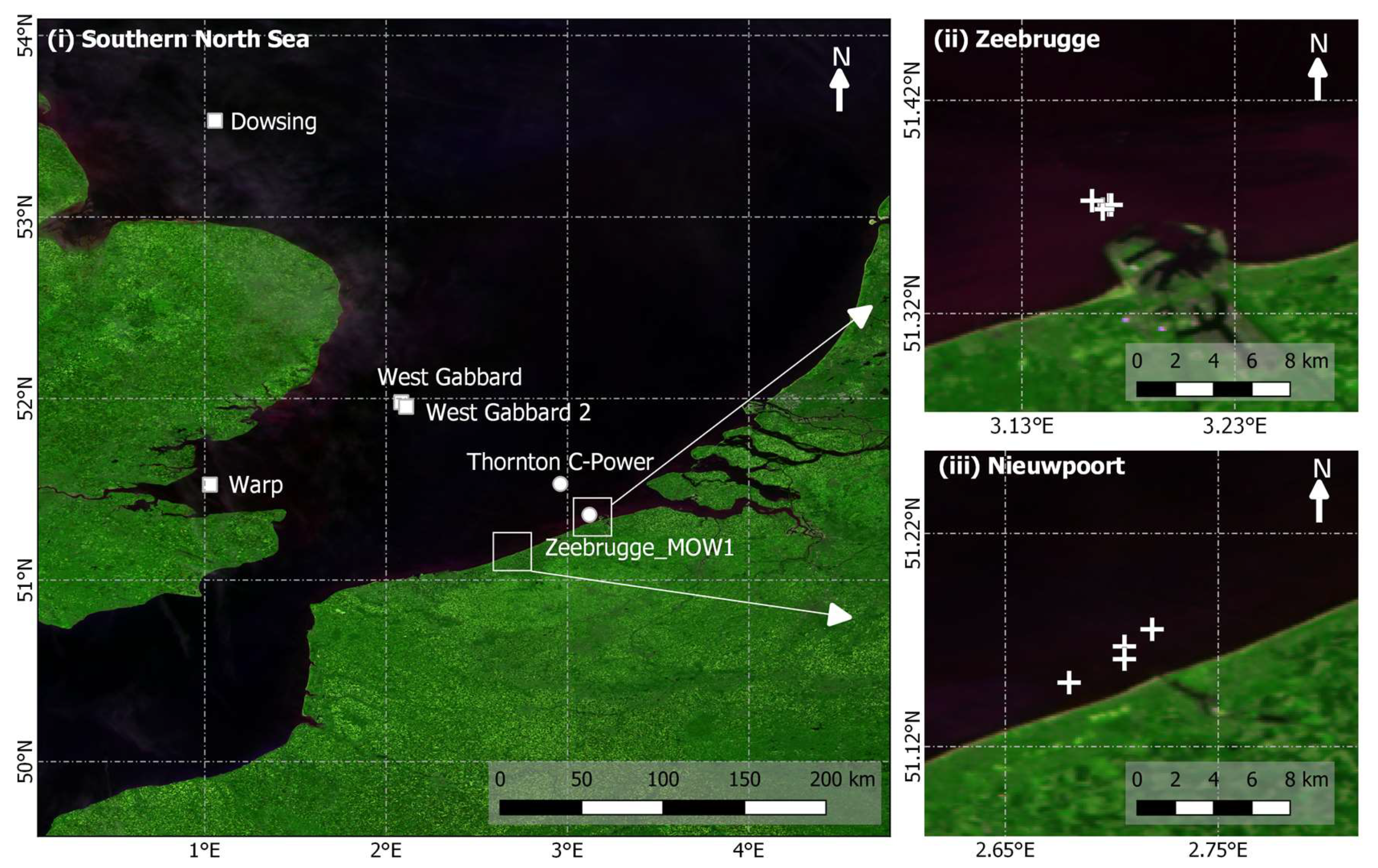
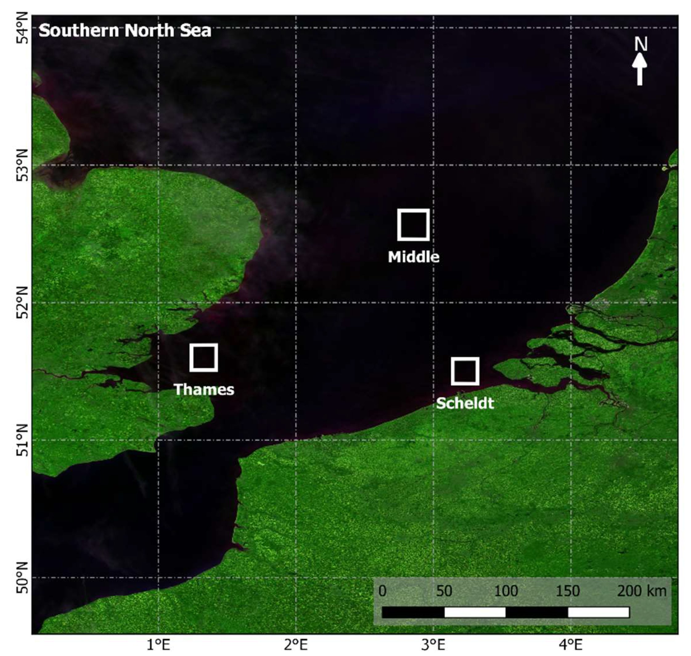
2.1. Study Area

This study focused on the southern part of the North Sea bounded by the east coast of England, the Strait of Dover and the Belgian and Dutch coast (50.7°–53.3°N; 0.1°–4.3°E), see Figure 1. The water depth is shallow (<50 m) with complex bathymetry patterns like ebb shoals (i.e., bulge of sand just seawards of an inlet), and a number of sand banks, tidal flats and shore connected ridges in the most Southern part along the Belgian coast [17]. Capuzzo et al. (2015) [18] described the decrease in water clarity of the southern and central North Sea during the 20th century after analyzing an extensive set of Secchi depth measurements from various data bases. They indicated different hydrodynamic regions in the North Sea, see Figure 1: (i) the East Anglia Plume (EAP), an extended area along the east coast of England and basically stretching from the Humber river to the English Channel including the Thames estuary and crossing the North Sea all the way to the zone of fresh water influence along the most southern Wadden Islands; (ii) a zone of freshwater influence (FWI), stretching along the Dutch coast from the outflow of Meuse and Rhine going North to the German Bight; (iii) a permanently mixed (PMX) zone from the English Channel all along the Belgian and Dutch coast until the start of the fresh water influence zone; (iv) an area called the intermediate zone (INT) covering the areas in the southern North Sea that are not part of the previous zones and finally (v) a seasonally stratified (SSR) zone roughly north of the 54°N latitude line. Coastal erosion (e.g., at the Holderness coast), the fresh water inflow from a number of important rivers (Humber, Thames, Scheldt, Meuse and Rhine) carrying nutrients and pollutants, the availability of mobile sediments (both cohesive and non-cohesive), the considerable tidal forcing (meso to macro-tidal) and occasional storms, all give rise to a complex interaction of processes of sedimentation, resuspension and erosion in the coastal areas. Fettweis et al. (2007) [19] give measurements of sediment concentrations taken at about 3 m above the bottom ranging from 3 to nearly 300 mg/L averaged over a tidal cycle with maximum concentrations going up to nearly 1000 mg/L in the Belgian coastal area. There is a clear seasonal variation with higher concentrations in autumn and winter and lower concentrations in spring and summer. Sediment concentrations, aggregation and break-up of cohesive sediment flocs [20,21] depend on, but also have an influence on, turbulence characteristics and on the variation of the concentrations over the water depth. Notwithstanding the complexity and variability due to the many factors that influence the signal detected by the satellite, the spatial but also the temporal coverage (long time series) of satellite observations are very valuable to increase our understanding of the underlying processes.

2.2. PROBA-V Mission

PROBA-V is a small satellite, launched on 6 May 2013 and designed to bridge the gap in space-borne vegetation measurements between SPOT-VEGETATION (SPOT-VGT) and the Sentinel-3 satellites. The mission had a designed life span of 2.5 years, but the excellent instrument and platform performance extended this mission till March 2020 [22]. PROBA-V flies at an altitude of 820 km in a sun-synchronous orbit with local overpass time at launch of 10:45 h. The total field of view is 102°, which results in a swath of 2295 km and a near-daily coverage at a spatial resolution of 300 m. The central camera observes at a higher spatial resolution of 100 m, and provides a global coverage every 5 days.

Although the satellite is primarily an inland vegetation satellite, the high revisit time, coastal coverage and spectral quality [16] provide opportunities to expand its current use over coastal water applications. The spectral and radiometric specifications of PROBA-V, including band center, bandwidth and Signal-To-Noise (SNR) at reference radiance L_ref, are summarized in

Table 1. Spectral and radiometric specifications of Proba-V [23].

Band	Band Center (nm)	Bandwidth (nm)	SNR at Lref
B1—BLUE	463	46	155 at 111 W m−2 sr−1 μm−1
B2—RED	655	79	430 at 110 W m−2 sr−1 μm−1
B3—NIR	845	144	529 at 101 W m−2 sr−1 μm−1
B4—SWIR	1600	73	380 at 20 W m−2 sr−1 μm−1

.

2.3. PROBA-V Processing

Top-Of-Atmosphere (TOA) PROBA-V images from January 2016 until August 2017 were downloaded from http://proba-v.vgt.vito.be. Instead of using the nominal Top-Of-Canopy (TOC) products generated with the Simple Model for Atmospheric Correction (SMAC), the atmospheric correction was performed using an extension of the image correction for atmospheric effects (iCOR) tool [24], adapted for PROBA-V and allowing Aerosol Optical Thickness (AOT) retrieval over water. In the nominal SMAC correction, AOT is estimated using an optimization algorithm that utilizes a relation between TOA Normalized Difference Vegetation Index (NDVI) and the observed SWIR/BLUE reflectance [25]. This optimization approach is not applicable over low NDVI surfaces such as water. For these areas, SMAC makes use of a static latitudinal dependent AOT value. As this hampers the retrieval of accurate reflectance values over water surface, a dedicated marine atmospheric correction (i.e., adapted iCOR of De Keukelaere et al. (2018) [24]) was selected for this study.

The iCOR atmospheric correction provides water leaving radiance reflectance (${\mathsf{\rho }}_{\mathrm{w}}$) products, which are used to derive turbidity maps. Both atmospheric correction and turbidity retrieval are discussed more in detail in the next Section 2.3.1 and Section 2.3.2.

2.3.1. Atmospheric Correction

An extended version of iCOR performed the atmospheric correction of PROBA-V data to retrieve ${\mathsf{\rho }}_{\mathrm{w}}$. iCOR uses the Moderate-Resolution Atmospheric Radiance and Transmittance Model-5 “MODTRAN5” [26] for the radiative transfer calculations and works with Look-Up Tables (LUT) to speed up the process. The overall workflow of iCOR is described in De Keukelaere et al. (2018) [24]. The strength of iCOR is that it is a surface adaptive correction method: the method identifies whether a pixel is water or land and applies a dedicated correction. iCOR runs without user interaction and derives the input parameters from the image itself. The existing version of iCOR relies on a land-based AOT retrieval. To avoid errors in extrapolating these land-based AOT values over large distances (i.e., the North Sea), an extension in the code is made for PROBA-V, which includes a water-based AOT retrieval using the NIR–SWIR bands. The availability of a NIR (845 nm) and SWIR (1600 nm) band allows a NIR–SWIR black pixel approach [27]. The NIR–SWIR black pixel approach assumes that the contribution of in-water constituents in the SWIR and for clear water pixels also in NIR is zero due to the high absorption of pure water in this spectral region. Any signal detected by the sensor for these bands is consequently assumed to be caused by atmospheric effects.

In the first step, clear water pixels are identified using a threshold value, see Equation (1) [27]:

$$\frac{{\rho }_{cor}^{rayl}\left(SWIR\right)+0.005}{{\rho }_{cor}^{rayl}\left(NIR\right)}>0.8$$

(1)

with ${\rho }_{cor}^{rayl}$ Rayleigh corrected reflectance, calculated using the MODTRAN5 LUT. The ratio of the Rayleigh corrected reflectance in the NIR and SWIR band (Equation (2)) over these clear water pixels, was calculated:

$${ϵ}^{NIR,SWIR}={\rho }_{cor}^{rayl}\left(NIR\right)/{\rho }_{cor}^{rayl}\left(SWIR\right)$$

(2)

The median ${ϵ}^{NIR,SWIR}$ value of the clear water pixels within the image is used to determine the final aerosol type, by comparing the value with pre-computed tabulated values for a suite of standard MODTRAN aerosol models (rural, urban and maritime). The aerosol model for which ${ϵ}_{Model}^{NIR,SWIR}$ corresponds best to the retrieved median ${ϵ}^{NIR,SWIR}$ value is selected as the final aerosol type.

In the second step, pixel-based AOT values are derived from the signal detected in the SWIR band. To reduce unwanted effects caused by inherent noise in the SWIR band, a simple box-averaging spatial smoothing is applied on the PROBA-V SWIR band as suggested by Wang et al. (2012) [28]. The algorithm searches for the AOT value that yields a water leaving radiance reflectance signal of zero in the SWIR band.

2.3.2. Turbidity Algorithm

Turbidity maps (T), expressed in the Formazin Nephelometric Unit (FNU) are generated from the water leaving radiance reflectance in the PROBA-V (PV) RED band ${\mathsf{\rho }}_{\mathrm{w}}\left(\mathrm{RED}\right)$ using the semi-analytical turbidity algorithm of Nechad et al. (2009) [2], Equation (3).

$$\mathrm{T}=\frac{{\mathrm{A}}_{\mathrm{T}}^{\mathrm{PV},\mathrm{RED}}·{\mathsf{\rho }}_{\mathrm{w}}\left(\mathrm{RED}\right)}{\left(1-\frac{{\mathsf{\rho }}_{\mathrm{w}}\left(\mathrm{RED}\right)}{{\mathrm{C}}_{\mathrm{T}}^{\mathrm{PV},\mathrm{RED}}}\right)}[\mathrm{FNU}]$$

(3)

where ${\mathrm{A}}_{\mathrm{T}}^{\mathrm{PV},\mathrm{RED}}$ and ${\mathrm{C}}_{\mathrm{T}}^{\mathrm{PV},\mathrm{RED}}$ are two wavelength-dependent calibration coefficients. These coefficients were calculated to match the PROBA-V RED band by first spectrally resampling the ${\mathrm{A}}_{\mathrm{T}}^{\mathsf{\lambda }}$ and ${\mathrm{C}}_{\mathrm{T}}^{\mathsf{\lambda }}$ coefficients tabulated at 2.5 nm resolution values in Nechad et al (2009) [2] to the PROBA-V RED spectral band. In Dogliotti et al. (2015) [1] the improved ${\mathrm{A}}_{\mathrm{T}}^{\mathsf{\lambda }}$ and ${\mathrm{C}}_{\mathrm{T}}^{\mathsf{\lambda }}$ coefficients are calculated based on an extended in-situ dataset. However, these improved ${\mathrm{A}}_{\mathrm{T}}^{\mathsf{\lambda }}$ and ${\mathrm{C}}_{\mathrm{T}}^{\mathsf{\lambda }}$ coefficients were only reported for MODIS spectral bands. To include these improvements also in the PROBA-V turbidity algorithm, the spectrally resampled values retrieved from the hyperspectral ${\mathrm{A}}_{\mathrm{T}}^{\mathsf{\lambda }}$ and ${\mathrm{C}}_{\mathrm{T}}^{\mathsf{\lambda }}$ given in Nechad et al. (2009) [2] are adjusted considering the percentage change suggested by Dogliotti et al. (2015) [1] for corresponding MODIS bands. The resulting values are 237.89 for ${\mathrm{A}}_{\mathrm{T}}^{\mathrm{PV},\mathrm{RED}}$ and 0.17 for ${\mathrm{C}}_{\mathrm{T}}^{\mathrm{PV},\mathrm{RED}}$.

2.4. Validation

PROBA-V products are compared with reference data acquired from AERONET-OC measurements, CEFAS SmartBuoy data and water samples collected during dedicated field campaigns from the Rigid-Hulled Inflatable Boat (RHIB) Zeekat. Figure 2 gives an overview of all sampling locations. The next paragraphs describe each of these validation datasets more in detail.

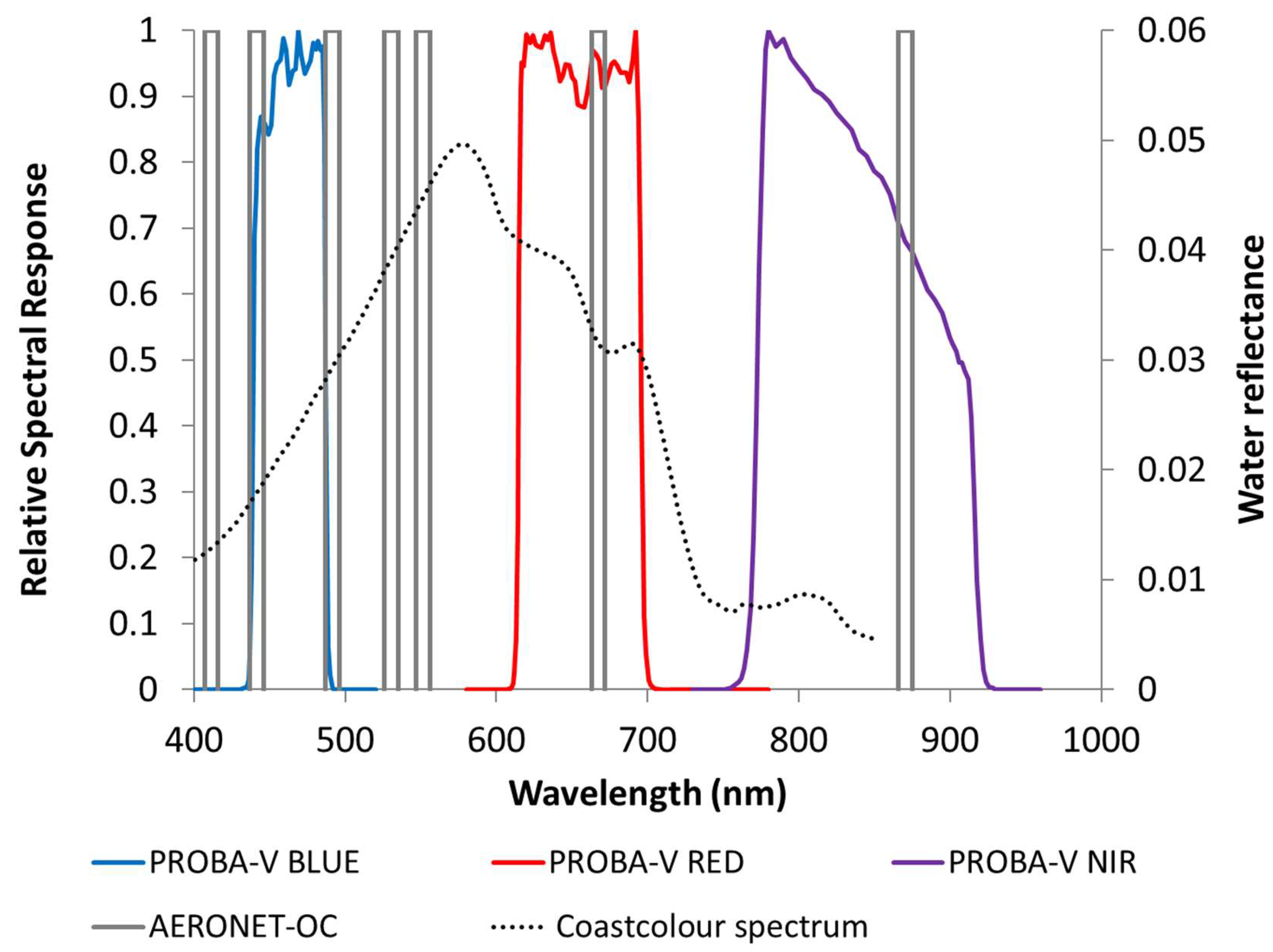
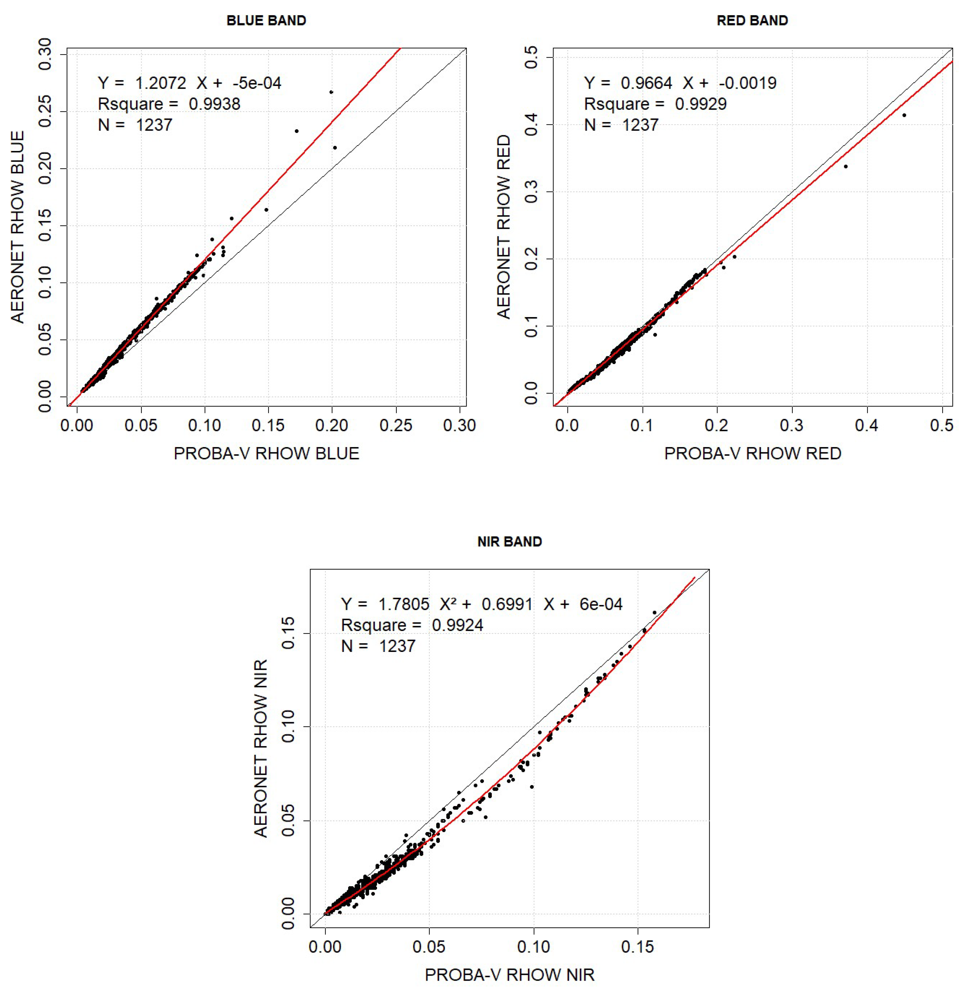
2.4.1. Water leaving Radiance Reflectance Validation with AERONET-OC

The North Sea is equipped with two AERONET-OC stations: (i) Zeebrugge-MOW1, in the coastal nearshore waters at a distance of ±4 km from land (51.36° N, 3.12° E), and (ii) Thornton_C-Power in clearer waters at 26 km from land (51.53° N, 2.96° E), see Figure 2. AERONET-OC stations conduct autonomous sun-photometer measurements and have a SeaWiFS Photometer Revision for Incident Surface Measurements (SeaPrism) installed, to measure sky-and sea-radiance in nine bands within the spectral range 412-1020 [29].

Available AERONET-OC Level 1.5 data (i.e., cloud-screened and quality controlled) from January 2016 till August 2017 were downloaded from (http://aeronet.gsfc.nasa.gov/). The normalized water leaving radiance (Lwn) data (mW/(cm² sr um)) from AERONET-OC was converted to ${\mathsf{\rho }}_{\mathrm{w}}$ using:

$${\mathsf{\rho }}_{\mathrm{w}}=\frac{Lwn}{F0}\ast pi$$

(4)

with $\mathrm{F}0$ being the exo-atmospheric solar irradiance (mW/(cm² um)) from Thuillier et al. (2003) [30]. Satellite and in-situ observations differ at spatial and temporal scale, which should be taken into account when directly comparing [31]. Ideally the in-situ observations are collected in homogenous areas [32] to minimize the effect of small-scale spatial variability on measured in-situ data and account for possible navigation errors in the satellite data. Mean PROBA-V reflectance values were extracted out of a 3 × 3 pixel box centered around the AERONET-OC stations. For homogeneous water masses, Bailey and Werdell (2006) [31] suggest a time window of 2 h around the satellite overpass for validation. Since the coastline of the Belgian North Sean is highly dynamic, we reduced the maximum allowed time difference between the satellite overpass and AERONET-OC measurements to 30 min. When multiple measurements were done within this time span, the mean value was calculated and used in further analysis. Furthermore, to enable this type of validation between the PROBA-V and the AERONET-OC sensors, it is key to quantify the differences in spectral band characteristics (i.e., central wavelength, band width and spectral response functions -SRF-, Figure 3) and compute a set of band shift coefficients to match the PROBA-V spectra to the in-situ spectra.

The AERONET-OC spectral band-set was optimized to match ocean color satellites (i.e., MODIS-AQUA and VIIRS), which were generally assumed to be ideal (square), 10 nm wide bands. When considering land sensors such as PROBA-V the differences in the center wavelength and bandwidth compared to the AERONET-OC band-set became significant. Figure 3 shows a comparison of the AERONET-OC and PROBA-V SRFs for their respective spectral bands providing an indication of the potential differences between radiometric measurements due to sensor characteristics.

The spectral shift corrections for the BLUE, RED and NIR bands of PROBA-V were determined based on hyperspectral ${\mathsf{\rho }}_{\mathrm{w}}$ in-situ database collected in the Southern North Sea from 2001 to 2016. Two research vessels, the Belgica and Zeeleeuw, were equipped with the above-water Trios (Rastede, Germany) Optical Systems (TRIOS), composed of three RAMSES hyper-spectral spectroradiometers. TRIOS sensors allow simultaneous measurements of the above-water downwelling irradiance (Ed), the upwelling radiance (Lsea) and the sky radiance (Lsky) to estimate the water-leaving radiance reflectance (${\mathsf{\rho }}_{\mathrm{w}}$):

$${\mathsf{\rho }}_{\mathrm{w}}=\frac{\mathrm{Lsea}-\mathrm{rf}\mathrm{Lsky}}{\mathrm{Ed}}\ast pi=\frac{\mathrm{Lw}}{\mathrm{Ed}}\ast pi$$

(5)

with rf the fraction of refracted Lsky at the air–sea interface (Fresnel reflectance). This latter is estimated from wind speed [34] in clear sky conditions, and set to 0.0265 in overcast conditions [35]. A set of 1243 hyperspectral measurements (spectral range: 350–900 nm, bandwidth: 2.5 nm) were available for further analysis.

Multi-spectral outputs were generated for the PROBA-V and AERONET-OC VNIR bands (490 nm, 670 nm and 870 nm) using their respective SRFs. The quantification of the differences between the in situ and satellite multi-spectral ${\mathsf{\rho }}_{\mathrm{w}}$ data sets enabled the calculation of simple band-shift correction coefficients to match-up the CIMEL-SeaPrism bands to the satellite sensor bands. Linear (Equation (6)) or polynomial (Equation (7)) shifts are suggested depending on the closest fit.

$${\mathsf{\rho }}_{\mathrm{W}}\left(\lambda \right)=a\ast {\mathsf{\rho }}_{\mathrm{W}}\left({\lambda }_0\right)+b$$

(6)

Or

$${\mathsf{\rho }}_{\mathrm{W}}\left(\lambda \right)=c\ast {\left[{\mathsf{\rho }}_{\mathrm{W}}\left({\lambda }_0\right)\right]}^2+d\ast {\mathsf{\rho }}_{\mathrm{W}}\left({\lambda }_0\right)+e$$

(7)

with a, b, c, d and e the band shift coefficients.

Figure 4 shows the scatterplots of simulated PROBA-V versus simulated AERONET-OC ${\mathsf{\rho }}_{\mathrm{w}}$ data for bands 490 nm, 670 nm and 870 nm. For the BLUE (490 nm) and RED (670 nm) a linear shift was suggested with a factors as 1.206 and 0.966 respectively in Equation (6), b factors were negligible. For the NIR band (870 nm) a polynomial shift was suggested with c- and d-factors being 1.781 and 0.699 respectively, the e-factor was negligible.

2.4.2. Turbidity Validation with In-Situ Measurements

CEFAS SmartBuoys

CEFAS SmartBuoys are automated, moored buoys, which allow high frequency measurements of multiple physical, chemical and biological variables [36]. One of the variables is turbidity, which is typically measured every 30 min at 1 m water depth. The data are freely available and can be downloaded from https://www.cefas.co.uk/cefas-data-hub/smartbuoys/. The SmartBuoys data underwent a quality assessment (QA), which includes flagging for biofouling, low power, etc. Figure 2 shows the location of the CEFAS SmartBuoys in the Southern North Sea. For each processed PROBA-V image the turbidity within a tile of a 3 by 3 macropixel around the SmartBuoy locations were extracted and compared with the CEFAS SmartBuoys turbidity values. Only the valid tiles were considered. Observations with a failure in the atmospheric correction or with a cloud percentage larger than 10% in the 1 km × 1 km region around the in-situ location were discarded. The threshold for the temporal offset between the time of the PROBA-V acquisition and CEFAS turbidity measurement was set to ±30 min, similar as with the AERONET-OC intercomparison.

Field Measurements

Between May 2016 and June 2017 field samples were collected at two locations along the Belgian coast: Nieuwpoort (51°10 N, 2°42 E) and Zeebrugge (51°22 N, 3°10 E). Figure 2 shows the location and date of the in-situ measurements. During clear sky days water samples of the surface were collected using the RHIB Zeekat. The aim was to take the samples within a time window of ±15 min around the PROBA-V overpass, due to practical reasons this was not always possible (e.g., on 14/09/2016 a time-difference of two hours was noted).

Table 2. Summary of the collected in-situ turbidity data. Date, location, latitude (°N), longitude (°E) and in-situ sampling time are given, together with the overpass time of PROBA-V times are expressing in local time.

Date	Location	Lat	Lon	In-Situ Sampling	PROBA-V Overpass
2016-05-04	Nieuwpoort	51.175	2.714	10:33–12:19	11:38
2016-05-19	Zeebrugge	51.370	3.170	11:18–13:14	11:01
2016-07-20	Zeebrugge	51.371	3.172	09:08–10:08	11:35
2016-08-17	Nieuwpoort	51.167	2.706	11:00–11:17	11:11
2016-08-25	Zeebrugge	51.369	3.168	12:05–12:13	11:39
2016-09-14	Nieuwpoort	51.161	2.707	11:22–13:01	10:51
2017-03-16	Zeebrugge	51.737	3.164	13:23–14:54	10:01
2017-05-10	Nieuwpoort	51.164	2.686	09:41–10:57	11:29

, summarizes the in-situ sampling locations and times. From the water samples turbidity measurements were taken with a HACH 2100Q IS handheld instrument, units expressed in FNU.

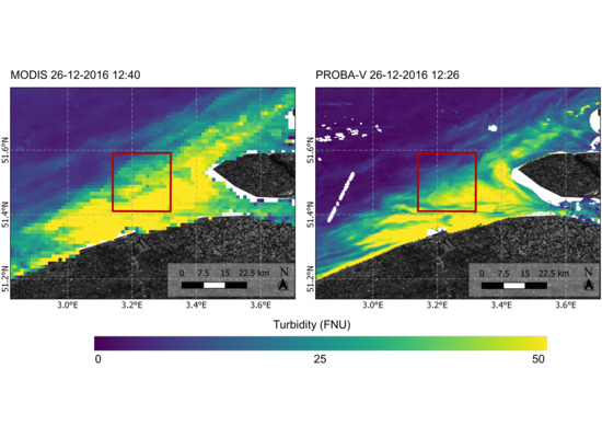
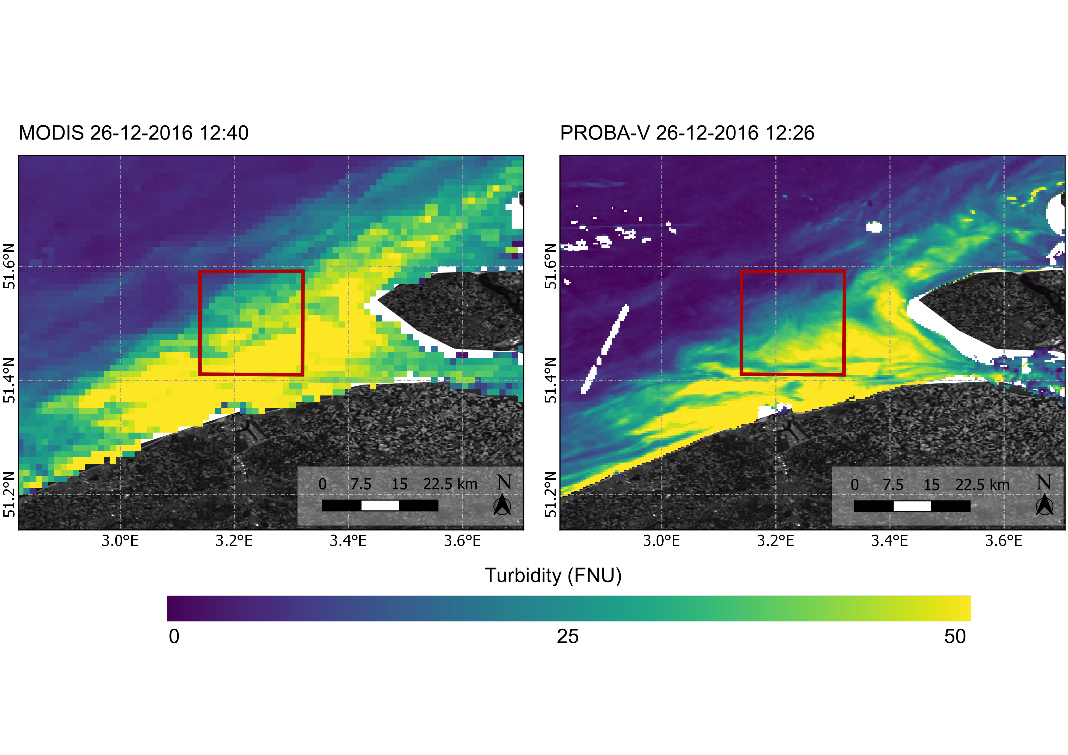
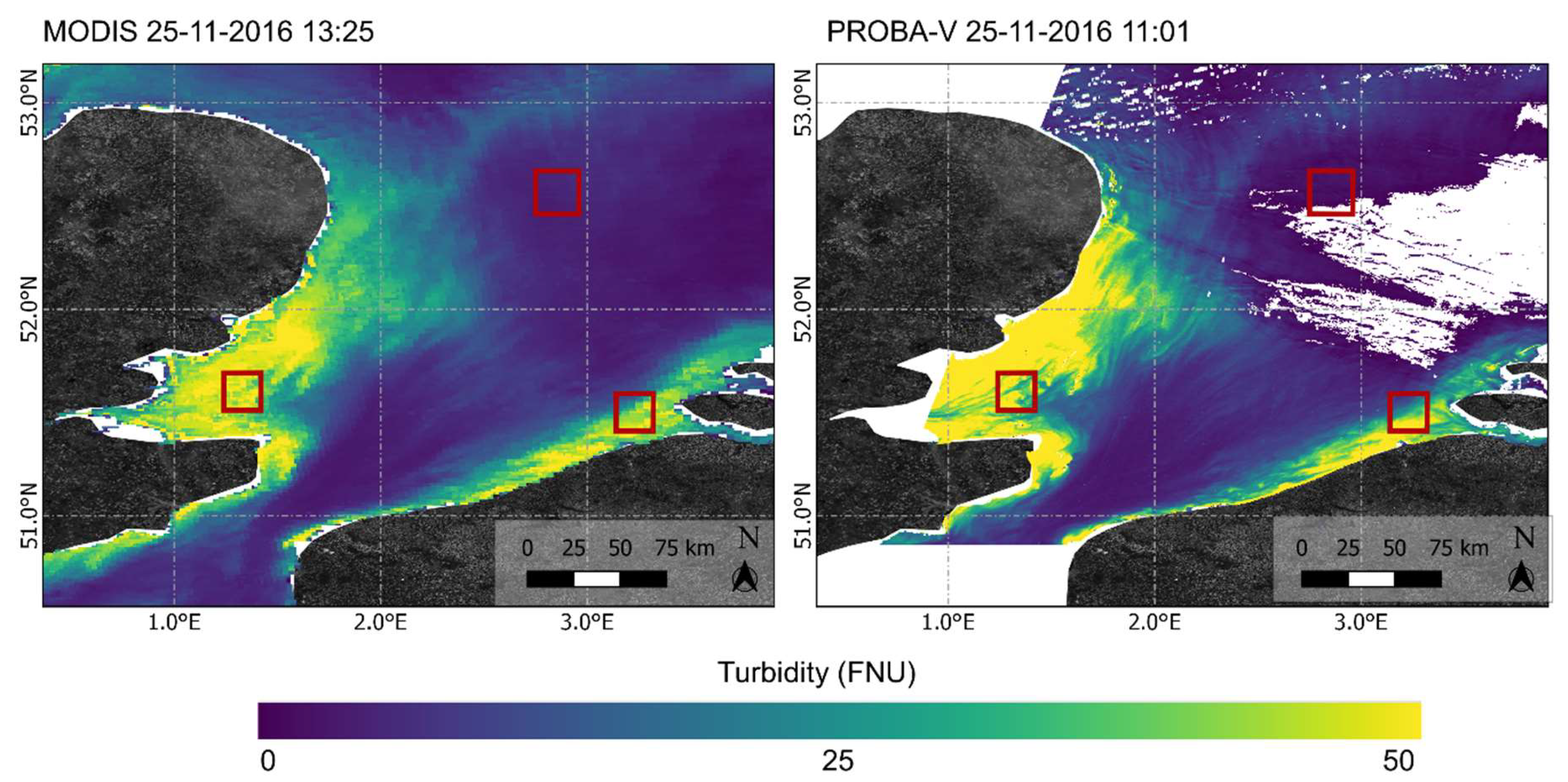
2.4.3. Turbidity Intercomparison with MODIS

Multiple studies have demonstrated the performance of the Moderate Resolution Imaging Spectroradiometer (MODIS) for water quality monitoring (e.g., [37]). The MODIS payload has been built under the TERRA satellite, launched in 1999 and onboard of the AQUA satellite, launched in 2002. The instrument has a viewing swath of 2.330 km and a temporal revisit time of ±1–2 days. The spectral imager measures in 36 spectral bands between 405 and 14,385 nm at three spatial resolutions (250 m, 500 m and 1000 m). In this study, MODIS AQUA data were used as a well-validated comparison dataset. The same time series as for PROBA-V was downloaded and processed to turbidity maps (i.e., January 2016–August 2017).

MODIS Processing

The atmospheric correction for MODIS data was performed using the SeaDAS/l2gen processing software following the Gordon and Wang approach for aerosol selection [38]. A Multi-scattering approach (aer_opt = −9) was selected, with a 2-band model selection using Shi and Wang’s turbidity index (1.30 [39]) to switch between SWIR and NIR. In clear waters, this method assumes no marine contribution in the NIR channels and uses the observed signal in two channels to select an aerosol model to extrapolate the aerosol reflectance across all bands. In waters where the marine contribution in the NIR cannot be assumed zero, an iterative bio-optical model is used to estimate NIR reflectances [40,41]. Observed TOA reflectances are corrected for ozone absorption and white caps. The Rayleigh reflectance is computed from geometry using look-up tables and adjusted for atmospheric pressure. After subtraction of the Rayleigh reflectance, Rayleigh and gas-corrected reflectance were obtained.

The aerosol reflectance was set to the Rayleigh and gas corrected reflectance in the longest used wavelength, which was 869 nm for MODIS. An aerosol model was estimated from the slope between the Rayleigh-corrected NIR reflectances [38], at 748 and 869 nm for MODIS. Based on the observed slope, the two best fitting aerosol models were selected from several tabulated models—currently 80 models. A weighted average of the selected models was used to extrapolate the aerosol reflectance to the other channels, which was then used to retrieve marine reflectance. The atmospheric correction was performed on MODIS L1b products, which were georeferenced and processed to sensor units (radiances) to generate L2 products. For a more thorough description, please refer to [42]. In the next step the semi-analytical algorithm of Nechad et al. (2009) [2] was applied to derive T (see Equation (3)) using the MODIS band of 645 nm, with $A_T^{MODIS-645}$ equals 394.7 and $C_T^{MODIS-645}$ equals 0.20175.

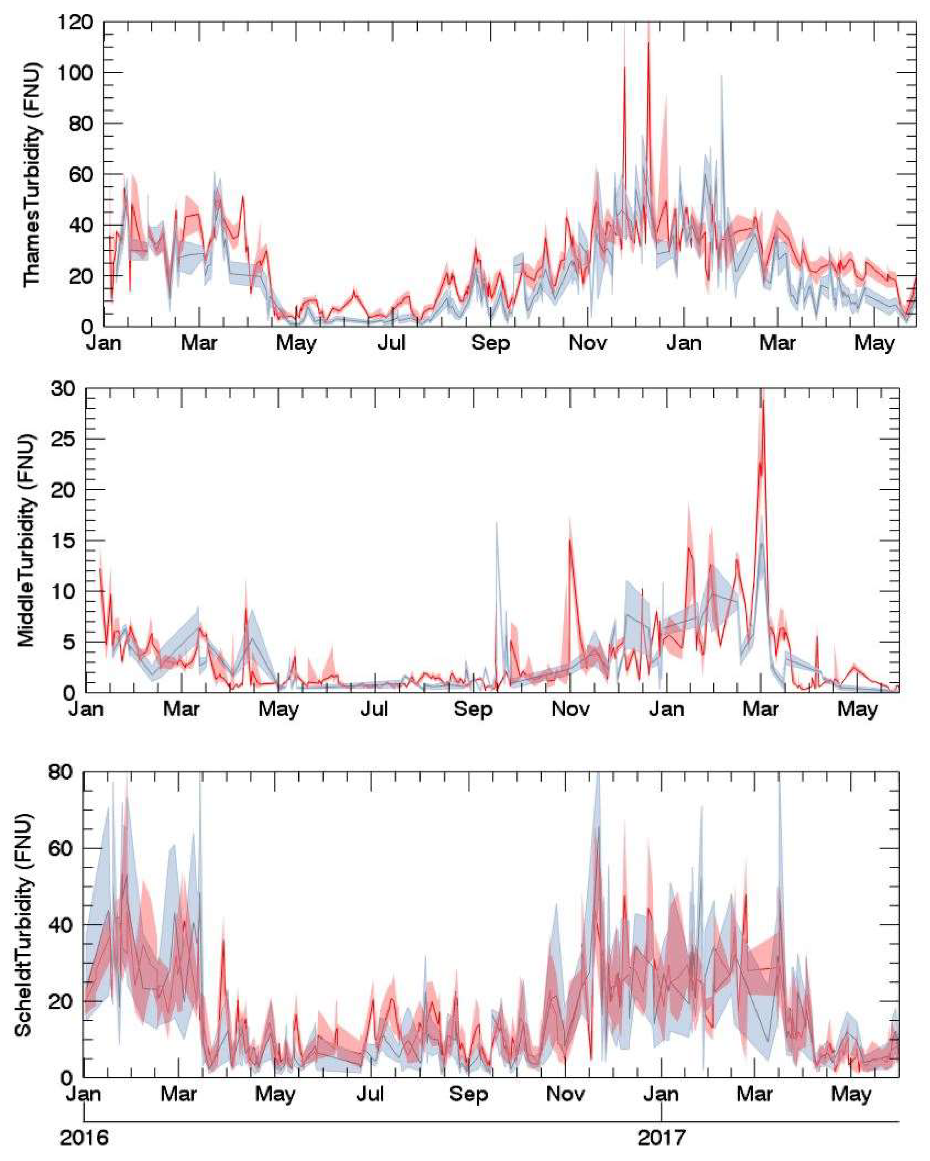
Time Series Intercomparison

Three subareas were defined in the North Sea, for which time series of turbidity values were extracted from PROBA-V and MODIS data, see Figure 5. The regions are about 400 km² and were defined in a function of varying expected sediment dynamics. The first Region of Interest (ROI 1) is located near the outlet of the Thames and, according to Capuzzo et al. (2015) [18], is situated at the start of East Anglia Plume. The Scheldt outlet region (ROI 2) is considered to be in the high dynamic well mixed zone [43]. Finally, an area in the middle of the North Sea was identified (ROI 3), which is located at the crossing of the permanently mixed and intermediate hydrodynamic regimes.

From each of these subsets the median values were derived, as well as the interquartile range (IQR). IQR is a measure of statistical dispersion and shows where the middle 50% of the values lie. When the total number of invalid pixels (e.g., high cloud cover) within the box was higher than 50%, the value was discarded.

3. Results

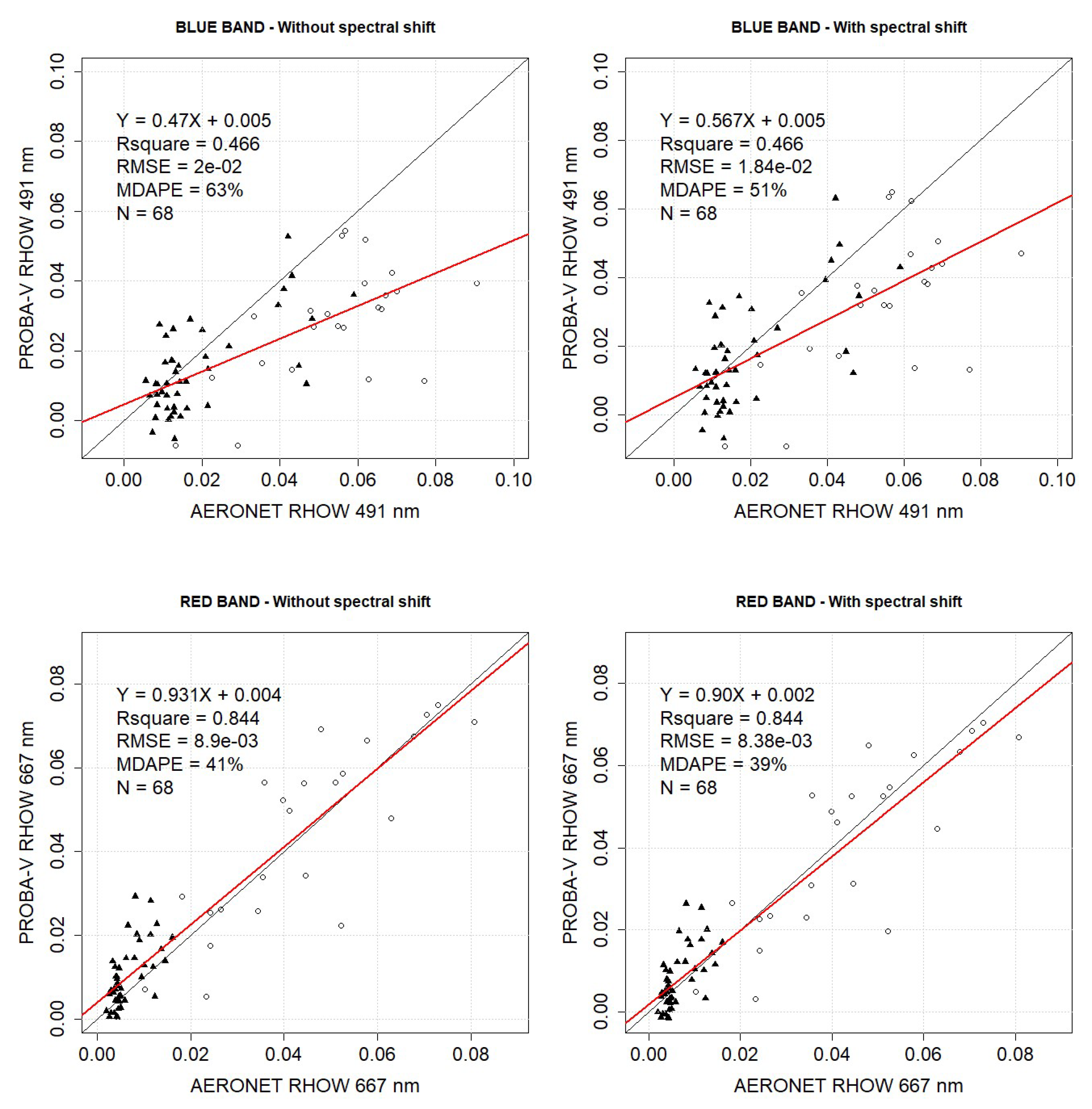
3.1. Water Leaving Radiance Reflectance Validation with AERONET-OC

Figure 6 shows scatterplots of ${\mathsf{\rho }}_{\mathrm{w}}$ data in BLUE, RED and NIR derived from PROBA-V and AERONET-OC for the Thornton_C-Power and Zeebrugge_MOW1 stations. Plots on the left show the results when no spectral shift correction was performed. Plots on the right underwent a spectral shift correction, as explained in Section 2.4.1. A strong correlation was found in the RED band with a coefficient of determination (R²) of 0.844, a slope relatively close to 1 (i.e., 0.9) and the Median Average Percentage Error (MDAPE) was 39%. BLUE and NIR bands yielded less satisfying results with a slope slightly higher than 0.5, an R² of respectively 0.47 and 0.17. Small improvements were noted after performing the spectral shift correction.

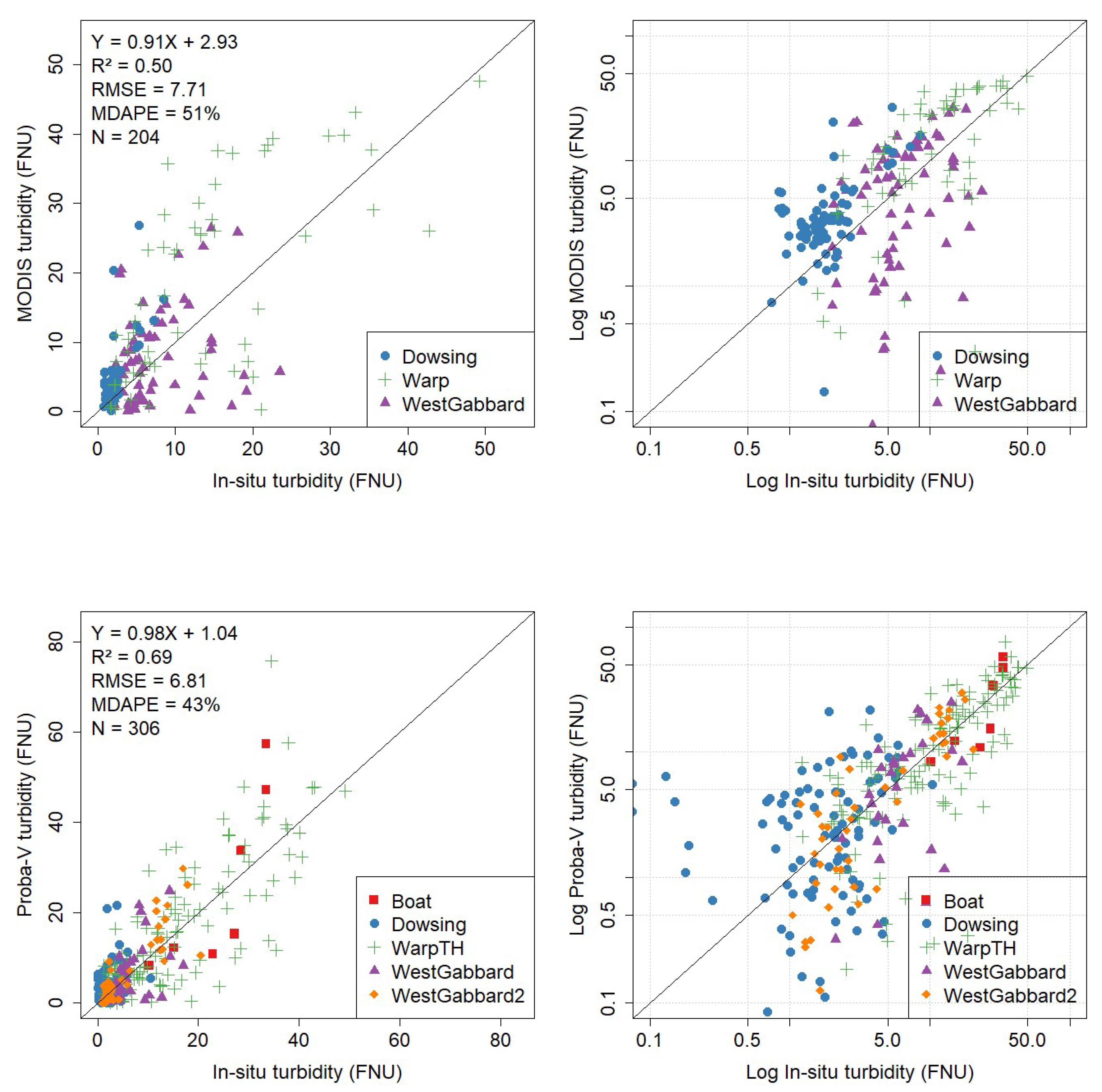
3.2. Turbidity Validation with In-Situ Measurements

The RED bands of MODIS and PROBA-V were used to derive the turbidity products. Figure 7 shows the scatterplots between MODIS or PROBA-V derived turbidity maps and in-situ data on linear and logarithmic (log) scales. The in-situ data consisted of measurements taken by CEFAS SmartBuoys (i.e., Dowsing, Warp and WestGabbard), and data sampled from a vessel in Zeebrugge and Nieuwpoort (see Section 2.3.2). The linear regression coefficients for MODIS yield a slope of 0.91 and offset of 2.93. The R² was 0.5, RMSE was 7.71 and MDAPE was 51%. PROBA-V shows a slightly better performance, but this could also be related to the larger set of match-ups (slope = 0.98, offset = 1.04, R² = 0.69, RMSE = 6.8 and MDAPE = 43%). The log plot indicates a larger percentage error for the lower turbidity values (more scattering) for both MODIS and PROBA-V. This observation was in line with expectations: low turbid waters have low water leaving radiance values, making the signal detected by the sensor more subject to influences of the atmosphere and/or SNR. Dowsing was located in the PMX zone (see Figure 1), West-Gabbard in the INT zone and Warp in the EAP zone. Boat measurements were all conducted in the PMX zone.

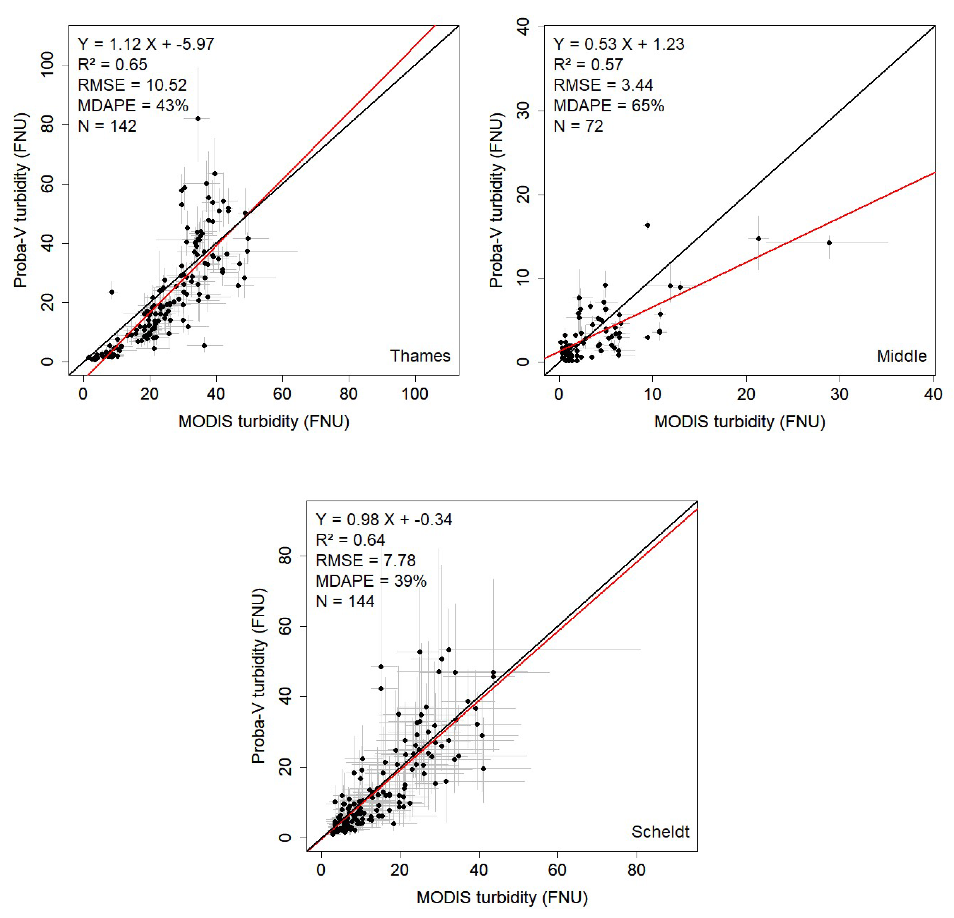
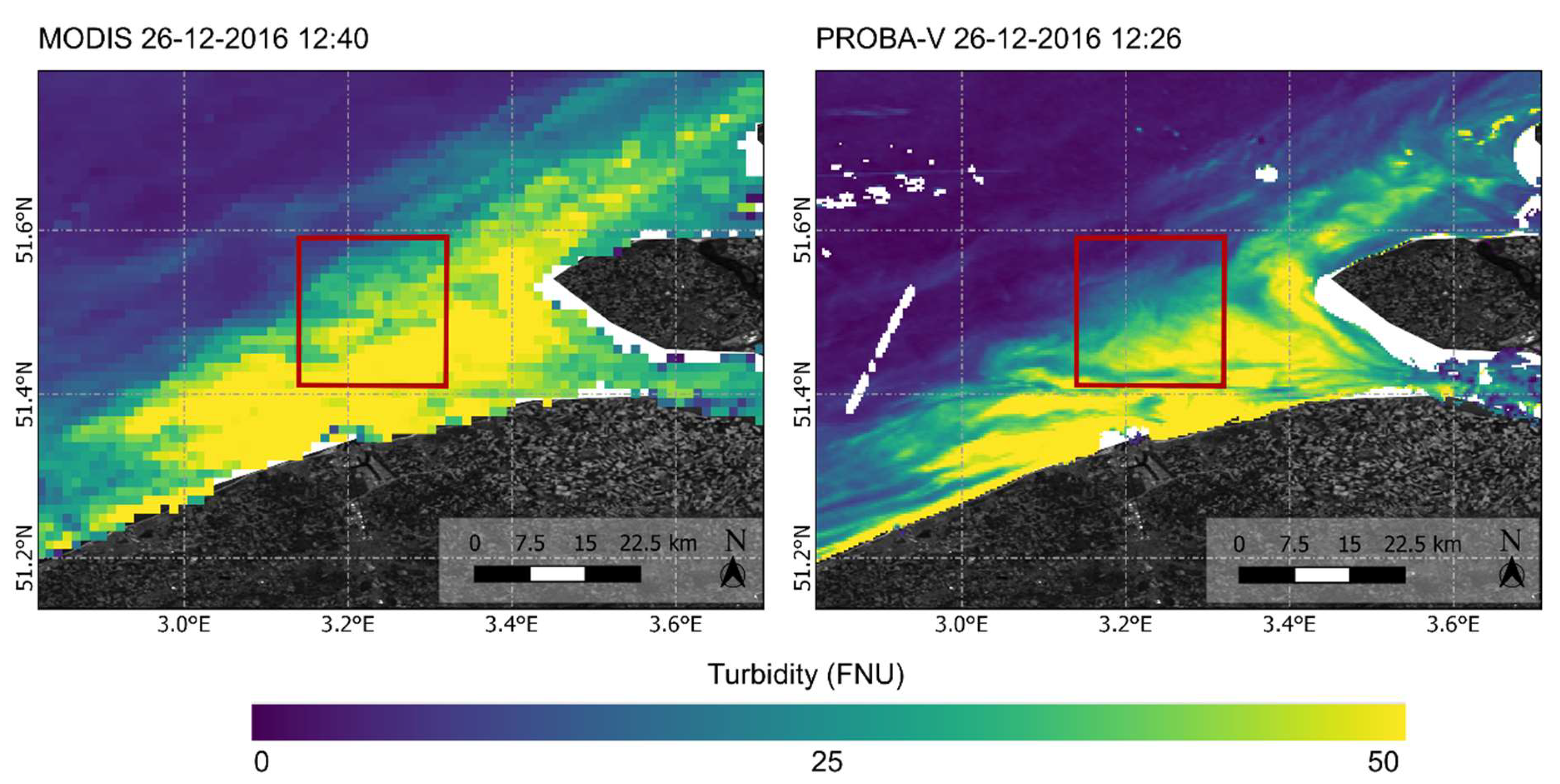
3.3. Turbidity Intercomparison with MODIS

A time-series of PROBA-V turbidity maps was compared with MODIS data for the three defined sub regions in the Southern North Sea (see Section 2.4.3 for the description of work). Figure 8 plots both dataset on a time scale. PROBA-V and MODIS follow similar patterns, which is mainly driven by seasonal and diurnal variation. Very often the seasonal pattern in wind and waves, with more storms in winter than summer, is put forward to explain the seasonality (e.g., [44]). The Middle of the North Sea, at the crossing of the permanently mixed and the intermediated hydrodynamic regime, has the clearest water. The turbidity near the outlet of the Thames River, at the start of the East Anglia Plume, is larger than for the Scheldt, located in the highly dynamic well mixed zone. For all three locations, turbidity increased in autumn and winter and is lower in spring and summer. The Scheldt region shows also a larger spread on the results: the interquartile range (IQR) was wider spread out around the median.

Scatterplots between PROBA-V and MODIS are depicted in Figure 9 for the three sub regions. The Scheldt outlet shows the best comparison with a slope of 0.98, offset of −0.34, R² of 0.64, RMSE of 7.78 and MDAPE of 39%. For the Thames outlet, MODIS seems to saturate between 50 and 60 FNU, while PROBA-V reached values up to 80 FNU. The slope was 1.12, while the offset was −5.97. In the Middle of the North Sea, MODIS shows two values higher than 20 FNU, all other observations were below 20 FNU for both PROBA-V as well as MODIS. The max allowed a time difference between MODIS and PROBA-V was set at 2 h [40]. Figure 10 and Figure 11 show a map of turbidity, generated using MODIS and PROBA-V data. While similar spatial turbidity patterns were visible, PROBA-V, with its higher spatial resolution (100 m) shows more detail.

4. Discussion

This is a first study that looked into PROBA-V data for water quality monitoring. PROBA-V is designed for global vegetation monitoring and was launched in 2013. The end of life of this mission is March 2020. Despite this near-ending mission, plenty of data was captured, archived and made available to users through the PROBA-V portal http://proba-v.vgt.vito.be. With this study we wanted to assess the asset of PROBA-V data for coastal water monitoring, although some more research and improvements might be necessary.

In the first step, an alternative atmospheric correction was proposed as the default SMAC-based atmospheric correction is not suitable for water targets. The default atmospheric correction relies on the relation between TOA NDVI values and observed TOA SWIR/BLUE reflectance to derive AOT values through optimization. For low reflectance values, this assumption is not valid. iCOR, previously tested on Landsat-8, Sentinel-2, e.g., [24,45,46], and Sentinel-3 [47] for inland and coastal waters, has been extended to PROBA-V and a NIR–SWIR black pixel approach [27] has been implemented. Spectral shift parameters were applied to the broad PROBA-V bands to allow a comparison with the narrow AERONET-OC bands. A strong correlation in RED band was found with a coefficient of determination (R²) of 0.844, a slope relatively close to 1 (i.e., 0.9) and the Median Average Percentage Error (MDAPE) was 39%. The BLUE and NIR bands yielded less satisfying results with a slope slightly higher than 0.5, an R² of respectively 0.47 and 0.17. The relatively poor performance in the BLUE band might be related to uncertainties in the atmospheric correction: the AOT was calculated using the SWIR band. Extrapolation of AOT from the SWIR to other bands, based on the defined aerosol model (Equation (2)), introduces uncertainty, which is largest for the BLUE band (largest wavelength distance). This in combination with the large field-of-view of the PROBA-V sensor with view zenith angles up to 60°. The NIR band on the other hand can be affected by sensor noise, due to the low radiance values over water in the NIR. Especially for the Thornton station, PROBA-V overestimates the measured reflectance in the NIR. A bad performance in the NIR band, when corrected with iCOR and compared with AERONET-OC, was also noted for Sentinel-2 and Landsat-8 [27]. For all bands, the spectral shift correction improved the results slightly. Although performing a spectral shift is necessary in theory, the resulting shift parameters in this test case were rather limited. The error and uncertainty linked to the atmospheric correction is higher than the spectral shift correction. iCOR makes use of pre-calculated MODTRAN-5 LUTs to enable operational processing and reduce processing time. In the previous iCOR version, as described in [27], only a rural aerosol model was included. This version incorporated additionally a desert and marine aerosol model. However, only one aerosol model is chosen for each scene. Furthermore, MODTRAN does not include correction for polarization, which becomes more important when looking to larger viewing angles [48].

In the next step, turbidity maps were generated using one single band, the RED band, using the method of Nechad et al. (2009). This method has shown good results in the North Sea in earlier studies [2]. The drawback of working with a single band algorithm is that errors made in the atmospheric correction will be further propagated into the end-products. In extremely high turbid regions, the RED band can show saturation and a switching between RED and NIR might be advised. Since the validation of water leaving reflectance data showed significantly better results for the RED band compared to BLUE and NIR, we kept to this single band approach. Note that turbidity is measured using different measuring techniques [16]. As mentioned, the turbidity derived from PROBA-V and MODIS makes use of the Nechad et al. (2009) algorithm. This semi-empirical relation is based on in-situ measurements made by the HACH ISO portable turbidity meter. This instrument uses the wavelength at 860 nm and records side scattering by particles at 90°. On the other hand, SmartBuoys make use of a Seapoint turbidity meter, with operating wavelength at 880 nm and recording light scattered by suspended particles between 15 and 150°. Although both are calibrated with standard Formazine suspensions, their response in natural waters might differ [49] because of the intrinsic difference in the measurement method.

5. Conclusions

Although PROBA-V data is currently mainly used for land monitoring, this study demonstrated its use for water applications. The nominal SMAC atmospheric correction was replaced with an adapted version of iCOR, since the optimization approach of SMAC is not applicable over water areas. iCOR was extended with a SWIR-based AOT retrieval. Comparison with AERONET-OC data show promising results, esp. in the RED band with a coefficient of determination of 0.844 and MDAPE of 39%. The BLUE and NIR band showed lower accuracies.

Starting from the RED band, turbidity values were derived. A comparison between CEFAS SmartBuoy and in-situ sampled data yielded a slope of 0.98 and offset of 1.04, while MODIS achieved a slope of 0.91 and offset of 2.93. A time series of PROBA-V was plotted over MODIS turbidity data for three subregions: the Thames outlet, the Middle of the North Sea and the Scheldt outlet. Both PROBA-V and MODIS showed an overall increase in turbidity in autumn and winter and a decrease in summer and spring, which is in line with earlier observations [13]. Same temporal as well as spatial patterns were detected. An intercomparison between PROBA-V and MODIS, yielded the best results for the Scheldt outlet, with a slope approaching 1 (0.98), offset of -0.34, R² of 0.64 and RMSE of 7.78.

These first results show that PROBA-V can be a valuable additional dataset for water quality monitoring, especially with regard to turbidity.

References

1. Dogliotti, A.; Ruddick, K.; Nechad, B.; Doxaran, D.; Knaeps, E. A single algorithm to retrieve turbidity from remotely-sensed data in all coastal and estuarine waters. Remote Sens. Environ. 2015, 156, 157–168. [Google Scholar] [CrossRef] [Green Version]
2. Nechad, B.; Ruddick, K.; Neukermans, G. Calibration and validation of a generic multisensor algorithm for mapping of turbidity in coastal waters. Proc. SPIE 2009, 7473, 1–11. [Google Scholar] [CrossRef]
3. Petus, C.; Chust, G.; Gohin, F.; Doxaran, D.; Froidefond, J.M.; Sagarminaga, Y. Estimating turbidity and total suspended matter in the Adour River plume (South Bay of Biscay) using MODIS 250-m imagery. Cont. Shelf Res. 2010, 30, 379–392. [Google Scholar] [CrossRef] [Green Version]
4. Moreno-Madrinan, M.J.; Al-Hamdan, M.Z.; Rickman, D.L.; Muller-Karger, F.E. Using the Surface Reflectance MODIS Terra Product to Estimate Turbidity in Tampa Bay, Florida. Remote Sens. 2010, 2, 2713–2728. [Google Scholar] [CrossRef]
5. Constantin, S.; Doxaran, D.; Constantinescu, S. Estimation of water turbidity and analysis of its spatio-temporal variability in the Danube River plume (Black Sea) using MODIS data. Cont. Shelf Res. 2016, 112, 14–30. [Google Scholar] [CrossRef]
6. Vanhellemont, Q.; Greenwood, N.; Ruddick, K. Validation of MERIS-derived turbidity and PAR attenuation using autonomous buoy data. In Proceedings of the 2013 European Space Agency Living Planet Symposium, Edinburgh, UK, 8–13 September 2013. [Google Scholar]
7. Gohin, F. Annual cycles of chlorophyll-a, non-algal suspended particulate matter, and turbidity from space and in-situ in coastal waters. Ocean Sci. 2011, 7, 705–732. [Google Scholar] [CrossRef] [Green Version]
8. Kyryliuk, D.; Kratzer, S. Evaluation of Sentinel-3A OLCI products derived using the Case-2 Regional CoastColour processor over the Baltic Sea. Sensors 2019, 19, 3609. [Google Scholar] [CrossRef] [Green Version]
9. Neukermans, G.; Ruddick, K.; Greenwood, N. Diurnal variability of turbidity and light attenuation in the southern North Sea from the SEVIRI geostationary sensor. Remote Sens. Environ. 2012, 124, 564–580. [Google Scholar] [CrossRef]
10. Vanhellemont, Q.; Ruddick, K. Turbid wakes associated with offshore wind turbines observed with Landsat 8. Remote Sens. Environ. 2014, 145, 105–115. [Google Scholar] [CrossRef] [Green Version]
11. Liu, L.W.; Wang, Y.M. Modelling reservoir turbidity using Landsat-8 satellite imagery by gene expression programming. Water 2019, 11, 1479. [Google Scholar] [CrossRef] [Green Version]
12. Kuhn, C.; Valerio, A.M.; Ward, N.; Loken, L.; Sawakuchi, H.O.; Kampel, M.; Richey, J.; Stadler, P.; Crawford, J.; Strieg, R.; et al. Performance of Landsat-8 and Sentinel-2 surface reflectance products for river remote sensing retrievals of chlorophyll-a and turbidity. Remote Sens. Environ. 2019, 224, 104–118. [Google Scholar] [CrossRef] [Green Version]
13. Caballero, I.; Steinmetz, F.; Navarro, G. Evaluation of the first year of operational Sentinel-2A data for retrieval of suspended solids in medium-to high-turbidity waters. Remote Sens. 2018, 10, 982. [Google Scholar] [CrossRef] [Green Version]
14. Bresciani, M.; Giardino, C.; Stroppiana, D.; Dessena, M.A.; Buscarinu, P.; Cabras, L.; Schenk, K.; Heege, T.; Bernet, H.; Bazdanis, G.; et al. Monitoring water quality in two dammed reservoirs from multispectral satellite data. Eur. J. Remote Sens. 2019, 52, 113–122. [Google Scholar] [CrossRef]
15. Sterckx, S.; Benhadj, I.; Duhoux, G.; Livens, S.; Dierckx, W.; Goor, E.; Adriaensen, S.; Heyns, W.; Van Hoof, K.; Strackx, G.; et al. The PROBA-V mission: Image processing and calibration. Int. J. Remote Sens. 2014, 35, 2565–2588. [Google Scholar] [CrossRef]
16. Knaeps, E.; Sterckx, S.; Bhatia, N.; Bi, Q.; Monbaliu, J.; Toorman, E.; Cattrrijsse, A.; De Keukelaere, K. Coastal Turbidity Monitoring using the PROBA-V Satellite. In Proceedings of the Coastal Dynamics 2017 Conference, Helsingør, Denmark, 12–16 June 2017; p. 19. [Google Scholar]
17. Anthony, E.J. Storms, shoreface morphodynamics, sand supply, and the accretion and erosion of coastal dune barriers in the southern North Sea. Geomorphology 2013, 199, 8–21. [Google Scholar] [CrossRef]
18. Capuzzo, E.; Stephens, D.; Silva, T.; Barry, J.; Forster, R.M. Decrease in water clarity of the southern and central North Sea during the 20th century. Global Change Biol. 2015, 21, 2206–2214. [Google Scholar] [CrossRef] [PubMed] [Green Version]
19. Fettweis, M.; Nechad, B.; Van den Eynde, D. An estimate of the suspended particulate matter (SPM) transport in the southern North Sea using SeaWiFS images, in situ measurements and numerical model results. Cont. Shelf Res. 2007, 27, 1568–1583. [Google Scholar] [CrossRef] [Green Version]
20. Lee, B.J.; Fettweis, M.; Toorman, E.; Moltz, F. Multimodality of a particle size distribution of cohesive suspended particulate matters in a coastal zone. J. Geophys. Res. 2012, 117, 1–17. [Google Scholar] [CrossRef]
21. Shen, X.; Toorman, E.A.; Lee, B.J.; Fettweis, M. Biophysical flocculation of suspended particulate matters in Belgian coastal zones. J. Hydrol. 2018, 567, 238–252. [Google Scholar] [CrossRef]
22. Wolters, E.; Dierckx, W.; Iordache, M.D.; Swinnen, E. PROBA-V Products User Manual V 3.01. 2018, v3.01, pp. 1–100. Available online: http://proba-v.vgt.vito.be/sites/proba-v.vgt.vito.be/files/products_user_manual.pdf (accessed on 29 January 2020).
23. Dierckx, W.; Sterckx, S.; Benhadj, I.; Livens, S.; Duhoux, G.; Van Achteren, T.; Francois, M.; Mellab, K.; Saint, G. PROBA-V mission for global vegetation monitoring: Standard products and image quality. Int. J. Remote Sens. 2014, 35, 2589–2614. [Google Scholar] [CrossRef]
24. De Keukelaere, L.; Sterckx, S.; Adriaensen, S.; Knaeps, E.; Reusen, I.; Giardino, C.; Bresciani, M.; Hunter, P.; Neil, C.; Van der Zande, D.; et al. Atmospheric correction of Landsat-8/OLI and Sentinel-2/MSI data using iCOR algorithm: Validation for coastal and inland waters. Eur. J. Remote Sens. 2018, 51, 525–542. [Google Scholar] [CrossRef] [Green Version]
25. Maisongrande, P.; Duchemin, B.; Dedieu, G. VEGETATION/SPOT: An operational mission for the Earth monitoring; presentation of new standard products. Int. J. Remote Sens. 2004, 25, 9–14. [Google Scholar] [CrossRef]
26. Berk, A.; Anderson, G.P.; Acharya, P.K.; Bernstein, L.S.; Muratov, L.; Lee, L.; Fox, M.; Adler-Golden, S.M.; Chetwynd, J.H.; Hoke, M.L.; et al. MODTRAN5: 2006 Update. Proc. SPIE 2006, 6233, 1–8. [Google Scholar] [CrossRef]
27. Vanhellemont, Q.; Ruddick, K. Advantages of high quality SWIR bands for ocean colour processing: Examples from Landsat-8. Remote Sens. Environ. 2015, 161, 89–106. [Google Scholar] [CrossRef] [Green Version]
28. Wang, M.; Shi, W.; Jiang, L. Atmospheric correction using near-infrared bands for satellite ocean color data processing in the turbid western Pacific region. Opt. Express 2012, 20, 741–753. [Google Scholar] [CrossRef]
29. Zibordi, G.; Holben, B.; Slutsker, I.; Giles, D.; D’Alimonte, D.; Mélin, F.; Berthon, J.-F.; Vandemarkn, D.; Feng, H.; Schuster, G.; et al. AERONET-OC: A network for the validation of ocean color primary products. J. Atmos. Ocean Technol. 2009, 26, 1634–1651. [Google Scholar] [CrossRef]
30. Thuillier, G.; Hers, M.; Simon, P.C.; Labs, D.; Mandel, H.; Gillotay, D. Observation of the solar spectral irradiance from 200 nm to 870 nm during the ATLAS 1 and ATLAS 2 missions by the SOLSPEC spectrometer. Metrologia 2003, 35, 689–695. [Google Scholar] [CrossRef]
31. Bailey, S.; Werdell, P.J. A multi-sensor approach for the on-orbit validation of ocean color satellite data products. Remote Sens. Environ. 2006, 102, 12–23. [Google Scholar] [CrossRef]
32. Gordon, H.R.; Clark, D.K.; Brown, J.W.; Brown, O.B.; Evans, R.H.; Broenkow, W.W. Phytoplankton pigment concentrations in the Middle Atlantic Bight: Comparison of ship determinations and CZCS estimates. Appl. Opt. 1983, 22, 20–36. [Google Scholar] [CrossRef]
33. Nechad, B.; Ruddick, K.; Schroeder, T.; Oubelkheir, K.; Blondeau-Patissier, D.; Cherukuru, N.; Brando, V.; Dekker, A.; Clementson, L.; Banks, A.C.; et al. CoastColour Round Robin data sets: A database to evaluate the performance of algorithms for the retrieval of water quality parameters in coastal waters. Earth Syst. Sci. Data 2015, 7, 319–348. [Google Scholar] [CrossRef] [Green Version]
34. Mobley, C.D. Estimation of the remote-sensing reflectance from above-surface measurements. Appl. Opt. 1999, 38, 7442. [Google Scholar] [CrossRef] [PubMed]
35. Ruddick, K.; De Cauwer, V.; Park, Y.-J.; Moore, G. Seaborne measurements of near infrared water-leaving reflectance: The similarity spectrum for turbid waters. Limnol. Oceanogr. 2006, 5, 1167–1179. [Google Scholar] [CrossRef] [Green Version]
36. Mills, D.K.; Laane, R.W.P.M.; Rees, J.M.; van der Looef, M.R.; Suylen, J.M.; Pearce, D.J.; Sivyer, D.B.; Heins, C.; Platt, K.; Rawlinson, M. Smartbuoy: A marine environmental monitoring buoy with a difference. Elsevier Oceanogr. Ser. 2003, 69, 311–316. [Google Scholar] [CrossRef]
37. Fettweis, M.; Nechad, B. Evaluation of in situ and remote sensing sampling methods for SPM concentrations, Belgian continental shelf (southern North Sea). Ocean Dyn. 2011, 61, 157–171. [Google Scholar] [CrossRef] [Green Version]
38. Gordon, H.R.; Wang, M. Retrieval of water-leaving radiance and aerosol optical thickness over the oceans with SeaWiFS: A preliminary algorithm. Appl. Opt. 1994, 33, 443–452. [Google Scholar] [CrossRef]
39. Shi, W.; Wang, M. Detection of turbid waters and absorbing aerosols for the MODIS ocean color data processing. Remote Sens. Environ. 2007, 110, 149–161. [Google Scholar] [CrossRef]
40. Bailey, S.W.; Franz, B.A.; Werdell, P.J. Estimation of near-infrared water-leaving reflectance for satellite ocean color data processing. Opt. Express 2010, 18, 7521–7527. [Google Scholar] [CrossRef]
41. Stumpf, R.P.; Werdell, P.J.; Arnone, R.A.; Gould, R.W.; Ransibrahmanakul, V. A partly coupled ocean–atmosphere model for retrieval of water-leaving radiance from SeaWiFS in coastal waters. NASA Tech. Memo. 2003, 206892, 51–59. [Google Scholar]
42. Mobley, C.D.; Werdell, J.; Franz, B.; Ahmad, Z.; Bailey, S. Atmospheric Correction for Satellite Ocean Color Radiometry; NASA/TM–2016-217551; NASA Goddard Space Flight Center: Greenbelt, MD, USA, 1 July 2016.
43. Fettweis, M.; Van den Eynde, D. The mud deposits and the high turbidity in the Belgian-Dutch coastal zone, southern bight of the North Sea. Cont. Shelf Res. 2003, 23, 669–691. [Google Scholar] [CrossRef]
44. Eleveld, M.A. Wind-induced resuspension in a shallow lake from Medium Resolution Imaging Spectrometer (MERIS) full-resolution reflectances. Water Resour. Res. 2012, 48, 1–13. [Google Scholar] [CrossRef] [Green Version]
45. Nurgiantoro, N.; Muliddin; Kurniadin, N.; Putra, A.; Azharuddin, M.; Hasan, J.; Hardianto; Langumadi, M. Assessment of atmospheric correction results by iCOR for MSI and OLI data on TSS concentration. In IOP Conf. Series: Earth Environment, Science, 389. Proceedings of the Geomatics International Conference, Surabaya, Indonesia, 21–22 August 2019; IOP Publishing Ltd.: Bristol, UK, 2019. [Google Scholar] [CrossRef]
46. Warren, M.; Simis, S.; Martinez-Vicente, V.; Poser, K.; Bresciani, M.; Alikas, K.; Spyrakos, E.; Giardino, C.; Ansper, A. Assessment of atmospheric correction algorithms for the Sentinel-2A MultiSpectral Imager over coastal and inland waters. Remote Sens. Environ. 2019, 225, 267–289. [Google Scholar] [CrossRef]
47. Kravitz, J.; Matthews, M.; Bernard, S.; Griffith, D. Application of Sentinel 3 OLCI for chl-a retrieval over small inland water targets: Successes and challenges. Remote Sens. Environ. 2020, 237, 1–21. [Google Scholar] [CrossRef]
48. Wang, M. Aerosol polarization effects on atmospheric correction and aerosol retrievals in ocean color remote sensing. Appl. Opt. 2006, 45, 8951–8963. [Google Scholar] [CrossRef] [PubMed]
49. Roesler, C.; Boss, E. In situ measurement of the inherent optical properties (IOPs) and potential for harmful algal bloom detection and coastal ecosystem observations. In Real-time Coastal Observing Systems for Marine Ecosystem Dynaimcs and Harmful Algal Blooms: Theory, Instrumentation and Modelling, 2nd ed.; Babin, M., Roesler, C., Cullen, J., Eds.; UNESCO: Paris, France, 2008; pp. 153–206. [Google Scholar]
Figure 1. (top) Project for On-Board Autonomy-Vegetation (PROBA-V) image of the region of interest and (bottom) the study area and the hydrodynamic regions: EAP, East Anglia Plume; FWI, freshwater influence; INT, intermediate; PXL, permanently mixed and SSR, seasonally stratified [18].
Remotesensing 12 00463 g001
Figure 2. Reference data used for the PROBA-V products validation, consisting of (i) two AERONET-OC stations: Thornton C-Power and Zeebrugge_MOW1 (dots), four CEFAS SmartBuoys: Dowsing, Warp, West Gabbard and West Gabbard2* (rectangles) and sampling from the RHIB Zeekat during field campaigns in (ii) Zeebrugge and (iii) Nieuwpoort (crosses).*The position of WestGabbard is slightly changed in May 2016; since then referred to as West Gabbard2
Remotesensing 12 00463 g002
Figure 3. PROBA-V and AERONET spectral bands in 400–1000 nm spectral range. The secondary Y-axis shows a sample in-situ measured hyperspectral ρ w spectrum of the North Sea extracted from the Coastcolour Round Robin dataset [33].
Remotesensing 12 00463 g003
Figure 4. Scatterplots of simulated ρ w from PROBA-V versus AERONET at selected center wavelengths. The determination coefficient (r2) and the slope characterize the linear regression for the BLUE and RED band. For the near infrared (NIR) band a polynomial fit is used.
Remotesensing 12 00463 g004
Figure 5. Demarcation of three subsites in the Southern North Sea used for time-series intercomparison: near the outlet of the Thames River, near the outlet of the Scheldt River and in the Middle of the North Sea.
Remotesensing 12 00463 g005
Figure 6. Regression plots of the water leaving reflectance from in situ (AERONET-OC) and from PROBA-V. On the left side, the results without spectral shift of the PROBA-V bands are plotted, while the images on the right shows the results after spectral shift correction. The triangles are results from the Thornton AERONET-OC station, the circles are results from the Zeebrugge-MOW AERONET-OC station. *_conv denotes that a spectral shift correction is applied to the PROBA-V reflectance in order to correct for the spectral response differences between PROBA-V and AERONET-OC. (R2 = coefficient of determination; RMSE = Root Mean Square Error; MDAPE = Median Absolute Percentage Error and N = total number observations).
Remotesensing 12 00463 g006aRemotesensing 12 00463 g006b
Figure 7. Regression plots between in-situ turbidity measurements (SmartBuoys and field data) and (top) MODIS or (bottom) PROBA-V derived turbidity values. On the left linear plots are given with the statistics (R2 = coefficient of determination, RMSE = Root Mean Square Error, MDAPE = Median Absolute Percentage Error, N = Number of observations). On the right, the data are plotted on a logarithmic scale. The solid black line is the 1:1 line.
Remotesensing 12 00463 g007
Figure 8. Time series of PROBA-V (grey) and MODIS (red) derived turbidity data from January 2016 to July 2017 for the subregion near the outlet of the Thames River (top), the middle of the Soutern North Sea (middle), and near the outlet of the Scheldt River (bottom). The light color around the solid lines show the IQR range (light grey for PROBA-V and light red for MODIS).
Remotesensing 12 00463 g008
Figure 9. Scatterplots between PROBA-V and MODIS turbidity for the Thames outlet (top left), Middle of the North Sea (top right) and Scheldt outlet (bottom). The solid black line is the 1:1 line, the grey lines show the IQR. The red line is the linear regression line (R2 = coefficient of determination, RMSE = Root Mean Square Error, MDAPE = Median Absolute Percentage Error and N = Number of observations).
Remotesensing 12 00463 g009
Figure 10. Turbidity map of the Scheldt outlet region generated with MODIS (left) and PROBA-V (right) data for the acquisition on 26/12/2016.
Remotesensing 12 00463 g010
Figure 11. Turbidity map of the Southern North Sea region generated with MODIS (left) and PROBA-V (right) data for the acquisition on 25/11/2016.
Remotesensing 12 00463 g011