Article

Quantifying Western U.S. Rangelands as Fractional Components with Multi-Resolution Remote Sensing and In Situ Data

1
Arctic Slope Federal Data Solutions, contractor to U.S. Geological Survey, Earth Resources Observation and Science Center, 47914 252nd Street, Sioux Falls, SD 57198, USA
2
U.S. Geological Survey, Earth Resources Observation and Science Center, 47914 252nd Street, Sioux Falls, SD 57198, USA
3
Formerly U.S. Geological Survey, Forest and Rangeland Ecosystem Science Center, Snake River Field Station, Boise, ID 83706, USA
4
KBR Contractor to U.S. Geological Survey, Earth Resources Observation and Science Center, 47914 252nd Street, Sioux Falls, SD 57198, USA
5
Formerly U.S. Geological Survey, Fort Collins Science Center, 2150 Centre Ave # C, Fort Collins, CO 8052
6
U.S. Department of the Interior, Bureau of Land Management, National Operations Center, Denver Federal Center, Building 50, Denver, CO 80225, USA
*
Author to whom correspondence should be addressed.
Remote Sens. 2020, 12(3), 412; https://doi.org/10.3390/rs12030412
Submission received: 23 December 2019 / Revised: 22 January 2020 / Accepted: 22 January 2020 / Published: 28 January 2020
(This article belongs to the Section Remote Sensing in Agriculture and Vegetation)

Abstract

:
Quantifying western U.S. rangelands as a series of fractional components with remote sensing provides a new way to understand these changing ecosystems. Nine rangeland ecosystem components, including percent shrub, sagebrush (Artemisia), big sagebrush, herbaceous, annual herbaceous, litter, and bare ground cover, along with sagebrush and shrub heights, were quantified at 30 m resolution. Extensive ground measurements, two scales of remote sensing data from commercial high-resolution satellites and Landsat 8, and regression tree models were used to create component predictions. In the mapped area (2,993,655 km²), bare ground averaged 45.5%, shrub 15.2%, sagebrush 4.3%, big sagebrush 2.9%, herbaceous 23.0%, annual herbaceous 4.2%, and litter 15.8%. Component accuracies using independent validation across all components averaged R2 values of 0.46 and an root mean squared error (RMSE) of 10.37, and cross-validation averaged R2 values of 0.72 and an RMSE of 5.09. Component composition strongly varies by Environmental Protection Agency (EPA) level III ecoregions (n = 32): 17 are bare ground dominant, 11 herbaceous dominant, and four shrub dominant. Sagebrush physically covers 90,950 km², or 4.3%, of our study area, but is present in 883,449 km², or 41.5%, of the mapped portion of our study area.

Graphical Abstract

1. Introduction

Arid and semiarid rangeland ecosystems comprise one-third of the Earth’s terrestrial environment and provide critical ecosystem services to human populations around the world [1,2]. Increasing direct and diffuse anthropogenic usage and threats on these ecosystems create an urgent need to better understand their biodiversity, function, mechanisms of change, biogeochemical cycles, and current distribution [3,4,5,6,7]. Rangelands are important sources of livestock forage, critical wildlife habitat, provide water resources, control erosion when managed properly, and modulate fire activity [8]. Rangelands in the western U.S. are highly variable, being composed of several major ecosystems, with each facing unique threats, and each with unique flora. Shrubland ecosystems include desert shrubland, California chaparral, salt desert shrubland, and sagebrush shrubland [8]. Grassland ecosystems dominate the short and mixed grass prairies of the Great Plains, annual grasslands in the Central Valley of California [9], and desert grasslands in the Sonoran and Chihuahuan Deserts.
The most common shrubland in the West, sagebrush, estimated to have once covered much of west and southwestern Canada, now occupies only approximately 56% of its historical range [10]. The contraction and degradation of the ecosystem is due to agricultural conversion, improper livestock grazing, increased fire intervals, invasive species, resource development, and climate change [11,12,13,14,15,16,17]. Ecosystem changes have impacted the flora and fauna, altered soil vitality, invasive species susceptibility, fire risk, and climate vulnerability [5,18,19,20,21,22,23]. Large-scale annual exotic grass invasion of species such as cheatgrass (Bromus tectorum) and medusahead (Taeniatherum caput-medusae), especially in the western parts of the ecosystem, have dramatically increased fire frequencies and made large regions vulnerable to permanently transitioning out of sagebrush shrubland [24,25]. At least 350 sagebrush-associated species have been identified as warranting concern [26], with sage grouse (Centrocercus urophasianus) receiving much of the conservation focus [13,27,28]. Continued change forces will likely further fragment and degrade remaining sagebrush areas [13,15]. Many of the other ecosystems of the West are subject to similar change agents including renewable and non-renewable energy production, mining, invasive species, land conversion, and woody plant expansion. Updated understanding of the abundance and quality of remaining sagebrush, and other rangeland, habitats is paramount to developing new scientific models and management tools [29,30].
Inventorying and quantifying western U.S. rangelands over large geographies with remote sensing has been evolving for many years. First-generation remote sensing efforts in the 1990s were produced on a state-by-state basis as land cover vegetation maps to support analysis of wildlife habitats and species distributions (i.e., gap analysis [31]). Next-generation efforts in the 2000s were part of more comprehensive database approaches developed across multi-state geographies to characterize rangelands into broad land cover classes through the National Land Cover Database [32] or represented as ecological systems by LANDFIRE [33]. Availability of these large area databases has facilitated better understanding of the general distribution of rangeland as land cover; however, these approaches have still proven inadequate to characterize rangelands with enough detail to facilitate local resource management and change monitoring. To be useful to monitoring agencies and on the ground operators, satellite monitoring of rangeland needs to correspond with units that these entities are familiar with and avoid calibration to small regions [34]. Hence, next-generation characterization work has focused on developing fractional predictions of shrub and grass components that can better localize characterization needs and improve the ability to monitor change across time [35,36,37,38,39,40]. For highly heterogeneous rangeland ecosystems, vegetation cover usually has a large range of variability, making it difficult to quantify effectively using only thematic land cover characterization. This new fractional component approach depends upon multi-scaled use of satellite imagery and intensive field sampling to capture rangelands as synergistic vegetative and bare ground components capable of then being re-assembled into a variety of habitat and monitoring applications [36,38,39]. However, to date, this approach which requires extensive field sampling, has not been applied to large regions of the western U.S.
This research effort characterizes western U.S. rangelands as a series of nine fractional cover components at 30 m resolution. Components include percent shrub, sagebrush, big sagebrush, herbaceous, annual herbaceous, litter, and bare ground cover, and sagebrush and shrub height in centimeters. Quantifying the landscape as a series of multiple components provides greater flexibility to create a complete range of habitat, management, and site indicator products and analysis. In this paper, we report the completion of our component characterization over much of the western U.S. This paper has three specific objectives. First, we report on total quantities and distributions of mapped components with associated validation accuracies. Second, we report U.S. Environmental Protection Agency (EPA) level III ecoregion [41] average component cover and climate associations. Third, we evaluate key fractional component proportions to better quantify and visualize component spatial distributions.

2. Materials and Methods

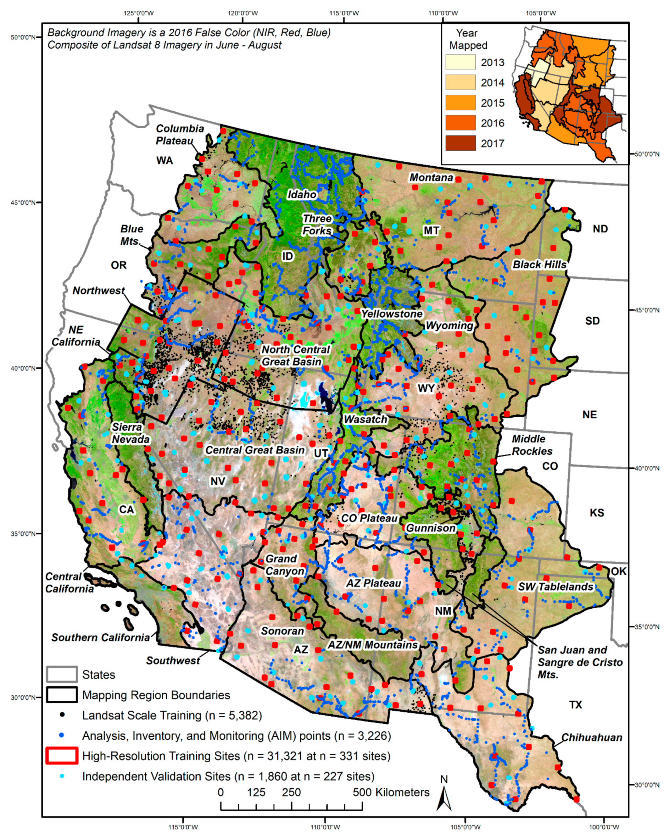
2.1. Study Area Description

This paper focuses on a large area of the western U.S. over a region covering parts of 16 states. We mapped the region as a series of 27 smaller mapping units over a 5-year span to accommodate field data collection logistics (Figure 1). Elevation varies across the region from a low of −86 m to a high of 4421 m. Vegetation varies widely and spans all altitudinal zones including alpine, subalpine, montane, foothills, and plains vegetation communities. In the alpine zone, vegetation communities are often above the tree line and consist of native shrub and perennial forb and grassland communities. Forest and woodland tree communities dominate the subalpine and montane zones, but substantial portions are occupied by herbaceous and shrubland communities, which often occur as an early successional response to disturbance before being ultimately replaced by trees. Shrub and herbaceous communities of the plains and foothills zones of the Great Plains and North American deserts EPA Level I ecoregions [41] constitute the greatest portion of our study area. Shrub vegetation is dominated by native shrub species, with herbaceous vegetation containing both native and exotic perennial and annual forb and grassland areas.

2.2. Methods

We quantified nine rangeland ecosystem components, including percent shrub, sagebrush, big sagebrush, herbaceous, annual herbaceous, litter, and bare ground cover, along with sagebrush and shrub heights, at 30 m resolution. This process was completed by independent mapping regions (Figure 1), which were subsequently mosaicked into a cohesive regional product. Mapping regions required extensive ground measurements for model training and validation, and two scales of remote sensing data. High-resolution satellite imagery (HRS) commercially available from WorldView-2, WorldView-3, QuickBird, or Pleaides resampled to 2 m nominal resolution provided the first scale for ground level interaction and measurement. Landsat 8 imagery acquired between 2013 and 2017 provided the second scale for landscape modeling. Mapping regions represented relatively similar ecological conditions and were identified by grouping one or more EPA level III ecoregions [41]. Mapping based on regions allowed for the collection of field and HRS data from the correct season of a single year. Also, since regression tree models tend to flatten the dynamic range of each component, dividing mapping into regions tends to limit this effect while exposing the regional regression tree model to more locally pertinent data, which also tends to improve model accuracy and relevancy. The main processing steps are described in Figure 2. Methods covering field measurement, image processing, component modeling, product masking, product validation and product analysis are described in detail below.

2.2.1. Field Sampling

Our field measurements created the foundation for all component modeling and validation. We targeted field measurements to coincide with HRS observation whenever possible to ensure correspondence in vegetation phenology. We used two field measurement protocols: a validation plot protocol using a randomized design for model assessment (described in the component validation section) and a more dynamic training plot protocol described here. Achieving acceptable model accuracy at the mapping region scale requires adequate distribution and quantity of training plots. To ensure training data collection was logistically feasible, field measurement was done on pre-selected HRS sites, which were located to collectively contain the full range of biophysical, ecological, and climatic conditions across each mapping region. HRS sites were strategically located in each mapping region through analysis of Landsat imagery, elevation, ecoregion boundaries, National Land Cover Database (NLCD) 2011 land cover, road accessibility, and public land access [39]. HRS images from the WorldView-2, WorldView-3, Pleiades-1, or QuickBird sensors were tasked for collection over each sample area at the approximate time the field crew was expected to be doing ground measurement. Hence, field crews typically had the satellite images to assist with analysis and placement of ground sampling. Further, any cloud or shadow cover present in the HRS image could be avoided in the field. If satellite images were not available, we used 1 m National Aerial Image Program (NAIP) imagery only to aid in field sampling. In these cases, HRS imagery was still used for component modeling. HRS sites were typically a single acquired image, approximately 15 by 15 km in size. All HRS imagery was ortho-rectified and resampled to 2 m nominal resolution prior to field data collection.
Initially, in the 2013 mapping region, we sampled predetermined locations on HRS deemed to be ecologically and spectrally critical to mapping with the goal of covering the range of cover values present for each component. This approach was cumbersome and quite slow. So, in later years (2014–2017), we evolved to an approach in which individual plots were dynamically selected for sampling, while still maintaining the goal of covering the range of cover values for each component. Specifically, on each HRS site, we simultaneously examined imagery displayed on a tablet (equipped with Environmental Systems Research Institute ArcMap and sub-meter accuracy global positioning system (GPS) units (Geneq inc. SX Blue II, Anjou, QB, Canada) and ground conditions. Criteria for plot selection included collecting adequate samples to represent the 1) cover histogram of each component, 2) topographic conditions; various elevation, aspect, and slopes, 3) range of management practices (i.e., grazed versus ungrazed, intensity of grazing, etc.), vegetation condition, or disturbances, and 5) the gross range of color and brightness of bare ground (referencing soil color charts when necessary) within each HRS site. Field plots needed to be homogenous over a large enough patch size to find the corresponding pixels on the HRS imagery, and so the vegetation patches measured were at minimum 2 m by 2 m in size. Overall, the sampling approach was dynamic based on the complexity of the sample area, available access, timing of the satellite collection and field sampling logistics. Although this approach required in-the-field judgment on where and how many samples should be collected, it dramatically reduced field sampling time and improved predictions over other more inflexible pre-determined methods used in 2013 by allowing ad hoc selection of plots by field personnel. To maintain consistency and rigor in the sampling procedures, the same field personnel collected data during the entire course of the research. Field personnel were extensively and regularly trained together to improve measurement consistency among personnel, HRS sites, and mapping regions and to calibrate field plot measurements to target components.
HRS plots varied in size and shape depending on the area of the patch being sampled, ranging from one 2 m pixel (4 m2) to 100 2 m pixels (400 m2). The average plot size on HRS imagery was approximately eight 2 m pixels (32 m2), which typically reflected the size of vegetation patch needed to gather reliable measurements. The goal was to make plots as large and homogeneous as possible, with a maximum size of 400 m2. Small, single pixel, plots were sometimes necessary to capture more extreme component values. Plots were edited/digitized in the field using ArcMap with component cover or height attributed to each plot on site. At each plot, we recorded an ocular estimate of cover for each component [36], with the total cover of all primary components (shrub, herbaceous, litter, and bare ground) and tree cover (not mapped) in a plot summing to 100%. We found that the potential reduction of accuracy and consistency in ocular estimation of component cover relative to pin drop methods, Daubenmire frames, etc., was more than compensated for in the vastly increased number of data points collected.
The shrub component encompassed numerous species and was discriminated by the presence of woody stems on a plant approximately <6 m tall (Table S1). The sagebrush component encompassed almost all species of sagebrush (Artemisia spp.) including big sagebrush (Artemisia tridentata), low sagebrush (Artemisia arbuscula), black sagebrush (Artemisia nova), three-tip sagebrush (Artemisia triparta), and silver sagebrush (Artemisia cana). However, we strived to exclude prairie sage (Artemisia frigida) and white sagebrush (Artemisia ludoviciana) from the sagebrush component as these suffrutescent shrubs were more spectrally and ecologically similar to herbaceous vegetation and subsequently grouped with the herbaceous component. Distinguishing the big sagebrush subspecies for sagebrush is important as big sagebrush is a critical indicator of sage grouse habit and landscape status/function. The big sagebrush component was dominated by big sagebrush (Artemisia tridentata spp.) but, because of spectral and ecological similarities, may also contain areas of three-tip sagebrush and silver sagebrush. The herbaceous component consisted of all grasses (live and residual standing), forbs, and cacti. The annual herbaceous component included only annual grasses and forbs (based on [42]), which in many portions of the study area were dominated by invasive grass species such as cheatgrass (Bromus tectorum), medusahead (Taeniatherum caput-medusae), red brome (Bromus rubens), or annual mustards such as tumble mustard (Sisymbrium altissimum), and tansy mustard (Descurainia pinnata). Annual herbaceous native species also are present in this component, but their cover is typically insignificant. The litter component included the combined cover of dead standing woody vegetation, detached plant and animal organic matter, and biological soil crusts. The bare ground component included any exposed soil or rocks. The average height of all shrubs and sagebrush in the plot was measured (in cm) using meter sticks on a representative shrub. Though we did not produce a fractional tree canopy cover map, a fractional component map developed by the U.S. Forest Service [43] was considered throughout production. See Table S1 for a complete description of each component.
We also collected additional training data outside of HRS sample areas to supplement the overall training pool. These Landsat-scale training plots (n = 5382) were designed to focus on large landscape features that may have been underrepresented in HRS sample areas, but still needed representation in the training pool (Figure 1). Using the same plot measurement technique employed with the high-resolution data collection, these plots were located directly on Landsat imagery. Additionally, Assessment, Inventory and Monitoring (AIM) data collected by the Bureau of Land Management (BLM) plots were added in mapping regions where available [44] (Figure 1). AIM data are standardized field observations of rangeland component cover collected to assess the condition and trend of natural resources. Further processing steps were required to ensure AIM data were directly relevant to our other training data, including aggregating the AIM classes into six components (bare ground, annual herbaceous, herbaceous, sagebrush, litter, and shrub). Next, we ensured AIM plots occurred on enough homogenous Landsat pixels to justify inclusion in our training data. Plots located on spectrally heterogeneous areas were deemed too diverse for training samples and were excluded. Following these procedures approximately half (n = 3226) of the available AIM data were included in model development.

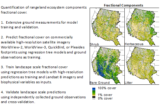
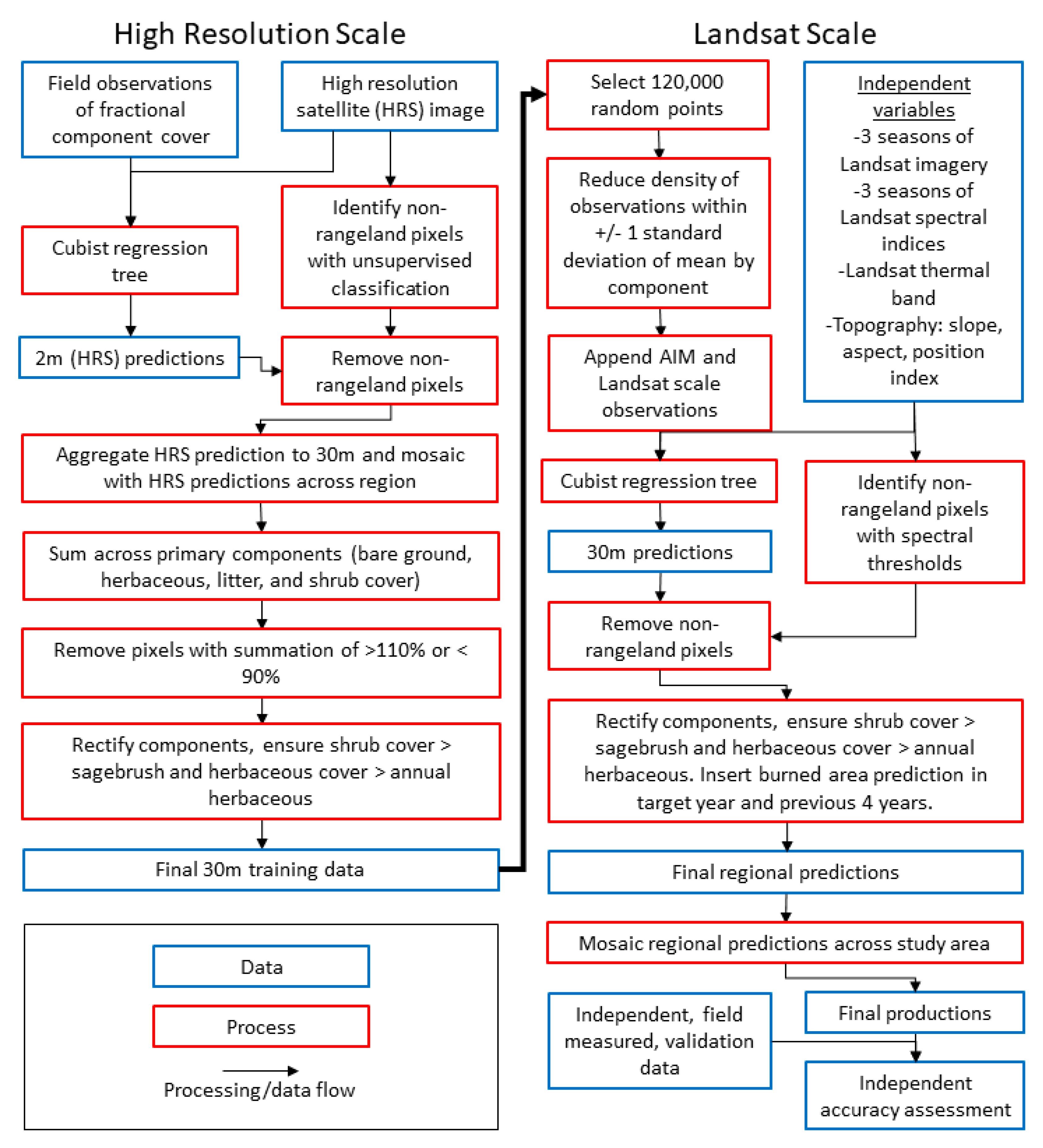
2.2.2. Satellite High-Resolution Image Processing and Modeling

Field data samples from within HRS sites were used as training data to predict fractional cover of nine different components on HRS images using a Cubist regression tree algorithm [45] following [38,39] at 2 m resolution. Our default condition choices were 10 committee members, 500 maximum rules and 10% extrapolation. Based on testing numerous settings, these parameters represented the best options to maximize the robustness of the models. All HRS bands were used in predictions applied across the entire HRS footprint for each of the nine components. Once predictions were completed, masking to exclude non-rangeland areas such as urban areas, agriculture, water bodies, and forests was performed. This exclusion process was typically done in three steps. First, an unsupervised classification on the HRS was completed to identify target clusters that represented forested areas for masking exclusion. Next, non-rangeland areas such as urban, water, and agricultural were identified using ancillary data and operator interpretation for exclusion. Finally, cloud or cloud shadow areas and snow were identified manually and excluded. The result was nine separate component predictions, with non-relevant areas excluded, ready for aggregation to 30 m scale model training data.

2.2.3. Landsat-Scale Image Processing and Modeling

For each mapping region, we aggregated the 2 m HRS predictions by averaging within 30 m pixels to serve as training data for regional predictions. Once aggregated to 30 m training pixels, data were filtered through summation of the four primary components (percent bare ground, shrub, herbaceous, and litter) for each pixel. Summation of the primary components should equal 100%, as they did so in all field plots. Deviation in summation from 100% suggests non-rangeland spectral contaminants in the pixel, or one or more inaccurate component predictions, which render the pixel less desirable for training. Hence, only pixels that had summation values that ranged from 90% to 110% were retained for potential training, with over 90% of the training data pool in each region meeting this criterion. Errors that exist in the HRS predictions can be propagated into the regional predictions but are critical to increasing the sample size and to scale plot observations up to Landsat scale. Additionally, HRS predictions form most of our training data pool (Figure 1). From the potential training pool for each region, 120,000 points were randomly selected as training for each component. Several, non-rangeland dominant ecoregions including the Arizona/New Mexico Mountains, Southern California, San Juan and Sangre de Cristo Mountains, Yellowstone, and Idaho regions were trained using a combination of Landsat-scale observations within the region and HRS predictions, Landsat-scale observations, and AIM data from a ~100 km buffer into the surrounding regions.
Training data for each region were stratified into three roughly equal bins of low, medium, and high values defined by the average and standard deviation (SD) of the pool. Values less than the average minus 1 SD were grouped into a low bin, values greater than the average plus 1 SD were grouped into a high bin, and the remaining values were considered in the middle bin. The final component training pool represented an approximately equal ratio of training data from each bin. Binning values helps regression tree models better represent high and low component cover values, spreading the prediction histogram [36,46]. Supplemental Landsat-scale training data collected outside HRS footprints were then added to the final pool of training for each component.
Landsat imagery was the key independent input for our fractional component models. We used U.S. Geological Survey (USGS) Earth Resources Observation and Science (EROS) Center Moderate Resolution Imaging Spectroradiometer (eMODIS) weekly Normalized Difference Vegetation Index (NDVI) data [47] to select the ideal dates of Landsat imagery for each region based on periods of best phenological separation among our primary components. For each region, we selected three image dates corresponding to green-up (spring), peak greenness (summer), and leaf off/post-peak (fall). While there is spatial variation in phenology within regions, we 1) strove to reduce this variation by delineating mapping regions based on common ecology, and 2) chose seasonal dates that represent the average phenology of regions. Though 8 day repeat Landsat datasets are available, we chose to maintain our methods as consistently as practical to those developed in 2013 prior to widespread adoption of automated image compositing methods such as Google Earth Engine (GEE). For the Great Basin and southwestern regions, nominal year 2013 and 2014 Landsat 8 images were used following the Multi-Resolution Land Characteristics (MRLC) image protocol [48] (Figure 1 inset). For the Wyoming/Montana region, nominal year 2015 Landsat 8 images were used following the EROS Science Processing Architecture (ESPA) image protocol [49]. For the Colorado and Columbia Plateaus, Blue Mountains, and Three Forks regions, nominal year 2016 Landsat 8 Analysis Ready Data products generated with version 3.1.2 of the Landsat Ecosystem Disturbance Adaptive Processing System (LEDAPS) were used [50]. Nominal year 2017 LEDAPS imagery was used for the Central California, Northeast California, Grand Canyon, Middle Rockies, and Southwest Tablelands regions. In the Wasatch Mountains, Arizona/New Mexico Mountains, Southern California, San Juan and Sangre de Cristo Mountains, Yellowstone, and Idaho regions, we used GEE to produce composite seasonal images from 2016–2018. All four protocols standardize Landsat imagery to at-satellite reflectance with Albers Equal Area projection. We created seasonal seamless imagery mosaics across Landsat path/rows in each region [39]. All seven Landsat 8 spectral bands (1–7) from each of three seasonal images were applied for the 2013–2015 mapping regions, with six Landsat 8 spectral bands (2–7) applied for the 2016–2017 regions. Band 1 was excluded in the 2016–2017 regions as we found that it provided little additional information relative to our mapping, and occasionally introduced noise. We also generated three spectral indices from each image: Normalized Difference Water Index (NDWI), Normalized Built-up Index (NBDI), and Soil Adjusted Vegetation Index (SAVI).
In addition to Landsat 8 imagery, other ancillary and image data were also key to the regression tree modeling. Ancillary data included slope and aspect products derived from a digital elevation model (DEM) to help stratify the model to appropriate topographical features. We also used the Landsat 8 thermal band (band 10, from the summer date), which functioned in our model as a DEM surrogate sensitive to summer topographic differences, which helped better stratify component elevation responses. Using a DEM product directly in our models produced model artifacts in preliminary predictions, but using the thermal band avoided these artifacts. We also used 30 m rescaled eMODIS data [47] when necessary to complement Landsat data seasonality, especially in regions with more dynamic phenology. Specifically, if regional analysis deemed the Landsat seasonal mosaics insufficiently captured important phenological stages, we created a 30 m Landsat 8 surrogate for the necessary seasonal date using downscaled eMODIS data. For this process, two methods were used based on regional applicability, either a regression tree [45] process [51] or the Spatial and Temporal Adaptive Reflectance Fusion Model (STARFM) algorithm [52]. Both created “Landsat-like” images in temporally missing portions of the seasonal Landsat record to better discriminate components. Analysis showed that inclusion of these images analogous to Landsat improved regional predictions, especially for herbaceous and annual herbaceous components, as evidenced by more robust regional independent and cross-validation statistics.
In the eastern and northern portions of the Montana region, where abundant herbaceous cover was commonly interspersed with low to moderate shrub cover (Figure 3, [53]), Landsat spectral data often produced insufficient component accuracies. To improve component discrimination, we developed a shrub/herbaceous index to improve regression tree modeling of the shrub and herbaceous components. This index was calculated as:
( shrub herbaceous   cover ) ( shrub + herbaceous   cover ) .
The index was applied to our 30 m scale training data, then modeled across the Montana region using Cubist regression trees for subsequent use as an independent variable in shrub and herbaceous component modeling. We found that inclusion of the shrub/herbaceous index in the independent variable stack resulted in a ~5% improvement in the accuracy assessment of the shrub and herbaceous cover components in the Montana region.
We mapped components individually with regression models produced by Cubist version 2.08 [45] for each of the nine components using all imagery, spectral indices, and ancillary data layers. Shrub and herbaceous secondary components (sagebrush, big sagebrush, and annual herbaceous components) were restricted to occur only in pixels with predicted values >0% of their respective primary component (i.e., parent component; Table S1). Shrub and sagebrush height were also restricted to occur in pixels with predicted values >0% in their respective parent component. To mitigate relatively rare cloudy areas in the Landsat 8 mosaics, a supplementary model that identified and ignored cloudy areas was completed. This model predicted components from the remaining cloud-free seasons to make component cover estimates in cloudy areas or mosaic artifacts in the original prediction.
To ensure recently burned areas were properly modeled, burned areas were identified using Geospatial Multi-Agency Coordination [54] fire perimeters. Fire events in the mapping year, and previous 4 years, were filled using a prediction generated with the season of imagery corresponding to post-burn conditions. In the Montana and Black Hills regions, data from the Monitoring Trends in Burn Severity fire perimeters after 2009 were also used to recode shrub, sagebrush, and big sagebrush to 0% within burn areas exhibiting high or moderate fire severity. We assumed after a severe fire that remaining live shrubs in the sagebrush ecosystem are rare [55,56], and since using the remote sensing prediction alone to identify remaining live shrubs created unacceptable commission error, setting the prediction to 0 in the year of the fire created less overall error.
Regional fractional cover maps were mosaicked to form a study area-wide component product. Each mapping region shared an overlap boundary with the adjacent region, and a cutline was used within a masked area or along a terrain feature to stitch regional predictions together.

2.2.4. Component Masking

We used two types of component masking to ensure we mapped only on relevant areas; non-rangeland and extent. Non-rangeland component masking removed non-rangeland portions of our study area, such as agricultural, urban, water bodies, and forest. Extent masking was designed to restrict component distribution to areas where the component occurs, which is only necessary for annual herbaceous, sagebrush, and big sagebrush. Extent masking was typically based on thresholds defined by a combination of elevation, aspect, and latitude. Specifically, these maps restricted the distribution of annual herbaceous at high elevation >~2300 m and sagebrush and big sagebrush at high elevation >~2700 m. In the Montana, Black Hills, and Wyoming regions, decision tree classifications were used to separate the mapping regions into occurrence and non-occurrence areas for sagebrush, big sagebrush, and annual herbaceous. Decision tree models were trained on occurrence from field plots and included seasonal Landsat 8 composites and ancillary data (slope and aspect). Final masks derived from the decision tree output were hand edited to ensure occurrence and non-occurrence areas were appropriate. Regions outside the occurrence area for a given component were re-coded to 0%.
For the non-rangeland mask, we identified forest areas using a combination of the NLCD 2016 fractional tree canopy cover product [43] with a threshold greater than 40% and NDVI or Modified Soil-Adjusted Vegetation Index (MSAVI) greenness thresholds. The MSAVI threshold remained relatively constant by mapping region season of imagery. In order to be masked as forest, all three seasons of Landsat image needed to be greater than the MSAVI threshold. Next, urban areas, major roads, snow, and ice were masked according to NLCD 2011 land cover classes [32]. Third, cultivated crop and pasture/hay fields were masked using a combination of the 2013 Cropland Data Layer for the U.S. from the U.S. Department of Agriculture, National Agricultural Statistics Service [57] and the NLCD 2011 agricultural classes, supplemented in certain regions with a combination of NDVI and MSAVI greenness thresholds. Fourth, open water areas in the Landsat mosaics were masked using the Normalized Difference Water Index (NDWI), defined as:
( green SWIR ) ( green + SWIR )
where SWIR is the shortwave infrared. A NDWI threshold (held constant among mapping region and season) was used to isolate water pixels, which was combined with the water class from NLCD 2011. Available HRS imagery was also used when available to help calibrate these masking models [39]. The final non-rangeland mask was validated by comparison to Landsat imagery and random samples from high-resolution images on Google Earth. Supplemental hand edits were then applied where issues needed correction.

2.3. Component Validation

We validated component predictions using three approaches: independent and cross-validation across the entire study area, and error maps within each mapping area. Independent validation was our primary validation approach, consisting of field measurements of component cover at stratified-random locations. Independent validation data were collected by the same field crews that collected field training samples to minimize human sample bias between training and validation measurements. Cross-validation data were obtained randomly from portions of HRS 30 m training sites withheld from model predictions.
Independent validation point placement used a stratified random design, with two levels of stratified restrictions to simplify logistics of field sampling. The first level of stratification randomly selected 15, 8 km in diameter, sites across each mapping region. First level sites excluded areas less than 30 km away from HRS training sites and other validation sites. The second level stratification randomly placed 6–10 points within each 8 km validation site (total n = 1860 points at n = 227 sites). Only sites on public land, between 100 and 1000 m from the nearest road, and in rangeland vegetation cover within each site were considered. The random points within a site were evenly allocated to three NDVI thresholds from a leaf-on Landsat image (low, medium, and high). Sites with relatively high spatial variance within a 90 m by 90 m patch (3 × 3 Landsat pixels) were excluded to minimize plot-pixel locational error. Using NDVI as a stratum ensured plot locations were distributed across the range of validation site productivity. At each validation point, we measured component cover in a 1 m2 quadrat every 5 m along a 30 m transect, averaging the seven observations for single plot values.
The secondary validation, cross-validation compared predicted component values to the values of 30 m training data at HRS sites withheld from model development. From each region, we selected 40,000 random pixels for evaluation. Results were proportionally weighted by the mapped area of each region to produce spatially balanced statistics for the entire study area. Validation parameters in both the independent and cross-validation included the coefficient of determination (R2), slope, root mean squared error (RMSE), and normalized RMSE (nRMSE). For the independent validation, we also calculated the 95% confidence limits of linear least-square regression models of field-measured versus predicted component cover, and the distance (in cover percent) between the upper and lower confidence limits.
A third validation approach used regression tree error maps generated in model development to characterize each component’s spatial error. This product was designed to assist users in understanding how model uncertainty is distributed spatially across the landscape and provide additional information to help determine the appropriate scale and confidence at which to apply the predictions. Component error maps from the Cubist regression modeling represented the mean absolute error between prediction and field-based estimates, based on rules, and were in the same unit as the prediction (either component percent error or centimeter height error). Error maps were not analyzed in the current study because we used them chiefly as internal reference, but they can be provided with each corresponding component prediction on a region-by-region basis.

2.4. Component Analysis

We analyzed the spatial distribution of components using multiple metrics. First, we evaluated the histograms of components across the study area to derive the area (km2) covered by each component, calculating by summing the fractional cover across pixels. We calculated the portion of the mapped area with predictions greater than zero cover/height and the average value by component. Next, we calculated the quartile statistics (1st quartile, mediation, 3rd quartile, maximum) for each component to generate box plots, with whiskers set to minimum and maximum values. Second, we determined EPA level III ecoregion average fractional component cover. For each level III ecoregion in the study area (n = 32), we calculated the 1981–2015 average water year (October–September) precipitation, maximum temperature, and minimum temperature using Daymet climate data [58]. Third, key component proportions were derived, including (1) shrub cover proportion of total rangeland vegetation (shrub plus herbaceous) cover, (2) annual herbaceous proportion of herbaceous cover, (3) big sagebrush proportion of sagebrush cover, and (4) other sagebrush (sagebrush minus big sagebrush) proportion of sagebrush cover.

3. Results

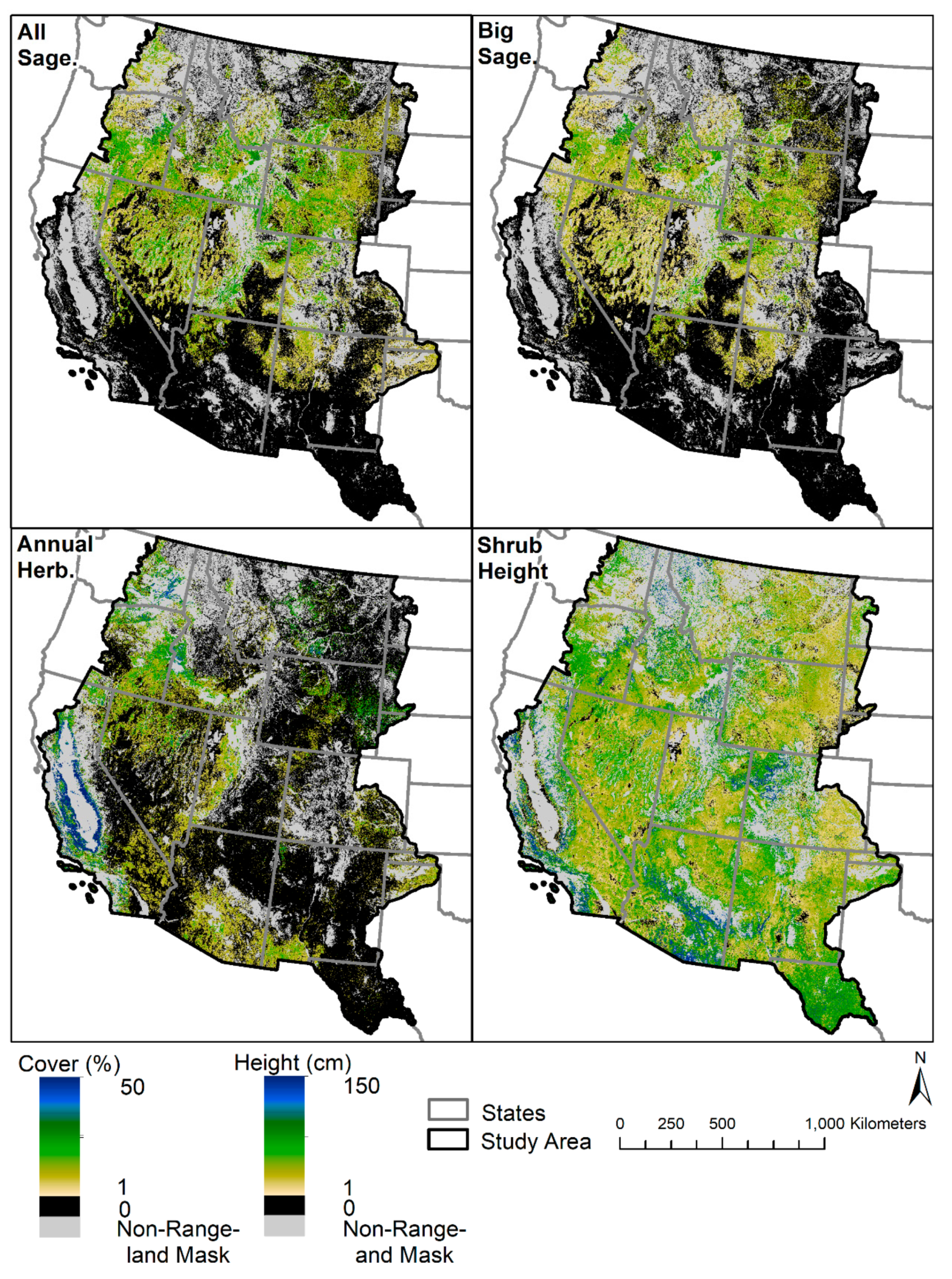
3.1. Component Predictions

A total geography of 2,993,655 km² was assessed—of which, 863,836 km² was in an exclusion mask, leaving 2,129,819 km² (71% of total study area) with the presence of at least one of the seven canopy components (i.e., mapped). When fractional predictions are converted to total area covered, bare ground occupies 968,792 km², herbaceous 490,517 km², litter 335,688 km², shrub 324,247 km², sagebrush 90,949 km², annual herbaceous 89,165 km², and big sagebrush 63,838 km² of the study area (Table 1). The balance of the mapped area, 10,575 km2, consists of tree canopy cover in a rangeland environment. Of the four primary components, shrub is present on 95.1% of the pixels, herbaceous on 99.5%, litter on 99.7% and bare ground on 99.9% of pixels. Sagebrush occurs on 41.5% of study area pixels. Annual herbaceous is present on the lowest proportion of pixels (30.1%) (Table 1).

3.2. Spatial Patterns

Training from 331 HRS sites was integrated into mapping the entire study area (Figure 1). Four commercial satellite sensors were tasked to collect imagery over HRS sites including 5 images from QuickBird, 96 from WorldView-2, 191 from WorldView-3, and 39 from Pleaides. For modeling components at the HRS level, 31,321 field training plots were collected across all HRS sites, averaging 95 plots per site. For the Landsat-scale models, an additional 3226 plots from BLM AIM data and 5382 Landsat field plots complemented HRS predictions (Figure 1).
Primary (Figure 3) and secondary (Figure 4) component maps follow expected ecological and biophysical patterns (e.g., shrub cover declines from west to east [19], sagebrush extent matches previous maps [59]). Shrub cover for example, is positively correlated with average water year precipitation (R2 = 0.14, p < 0.05), while bare ground is negatively correlated (R2 = 0.26, p < 0.05). Patterns related to disturbance history, land use, and topography are also evident. Fractional cover relationships among pixels are as expected. The fractional cover of herbaceous, for example, is strongly negatively related to bare ground (R2 = 0.57, p < 0.05) and shrub height is positively associated with shrub cover (R2 = 0.76, p < 0.05). All components, except bare ground and litter, have a distribution that is skewed to the right (Figure 5). Bare ground has a near normal distribution of fractional cover values, and litter cover is skewed slightly to the left. The median value of sagebrush, big sagebrush and annual herbaceous is 0% (Figure 4 and Figure 5).

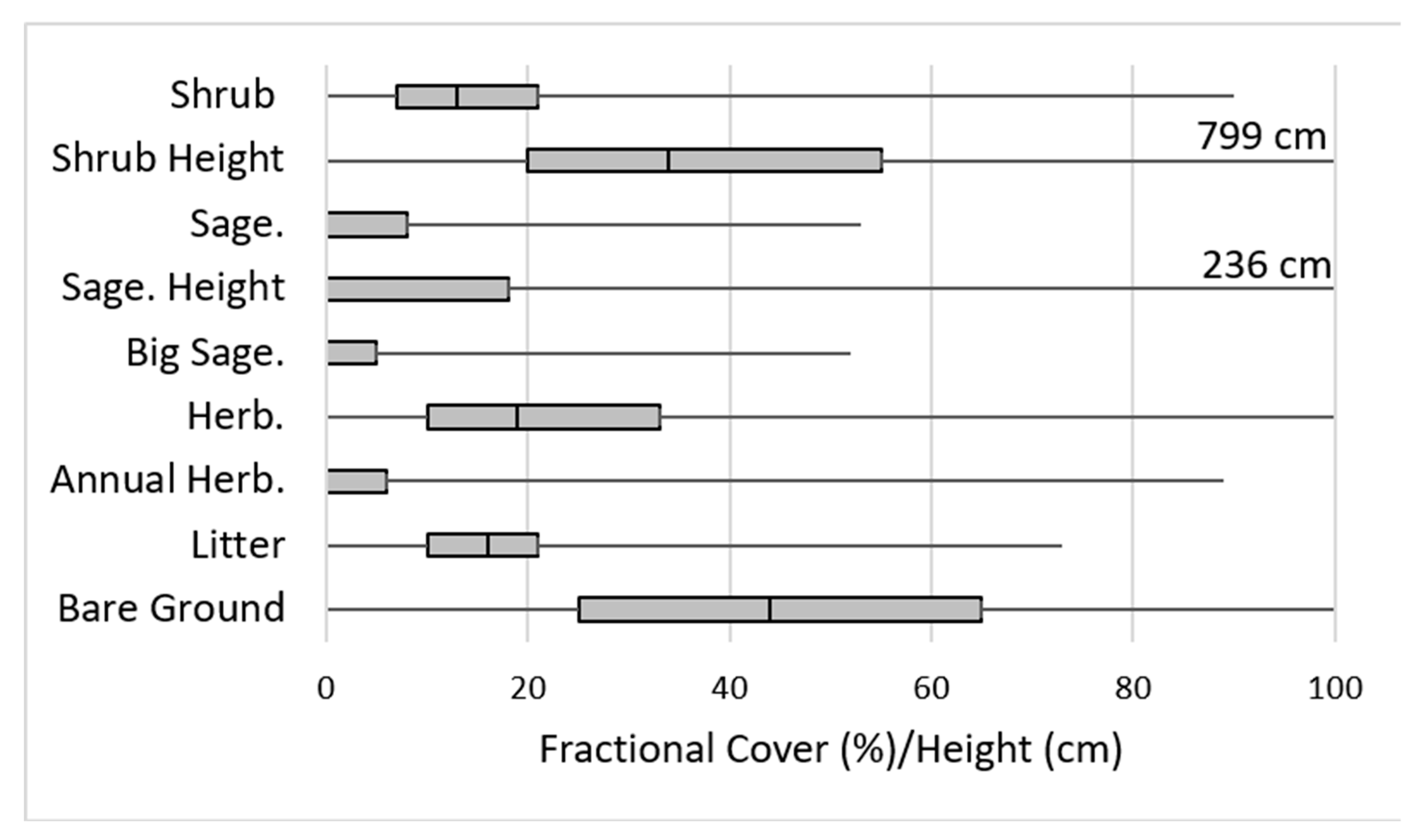
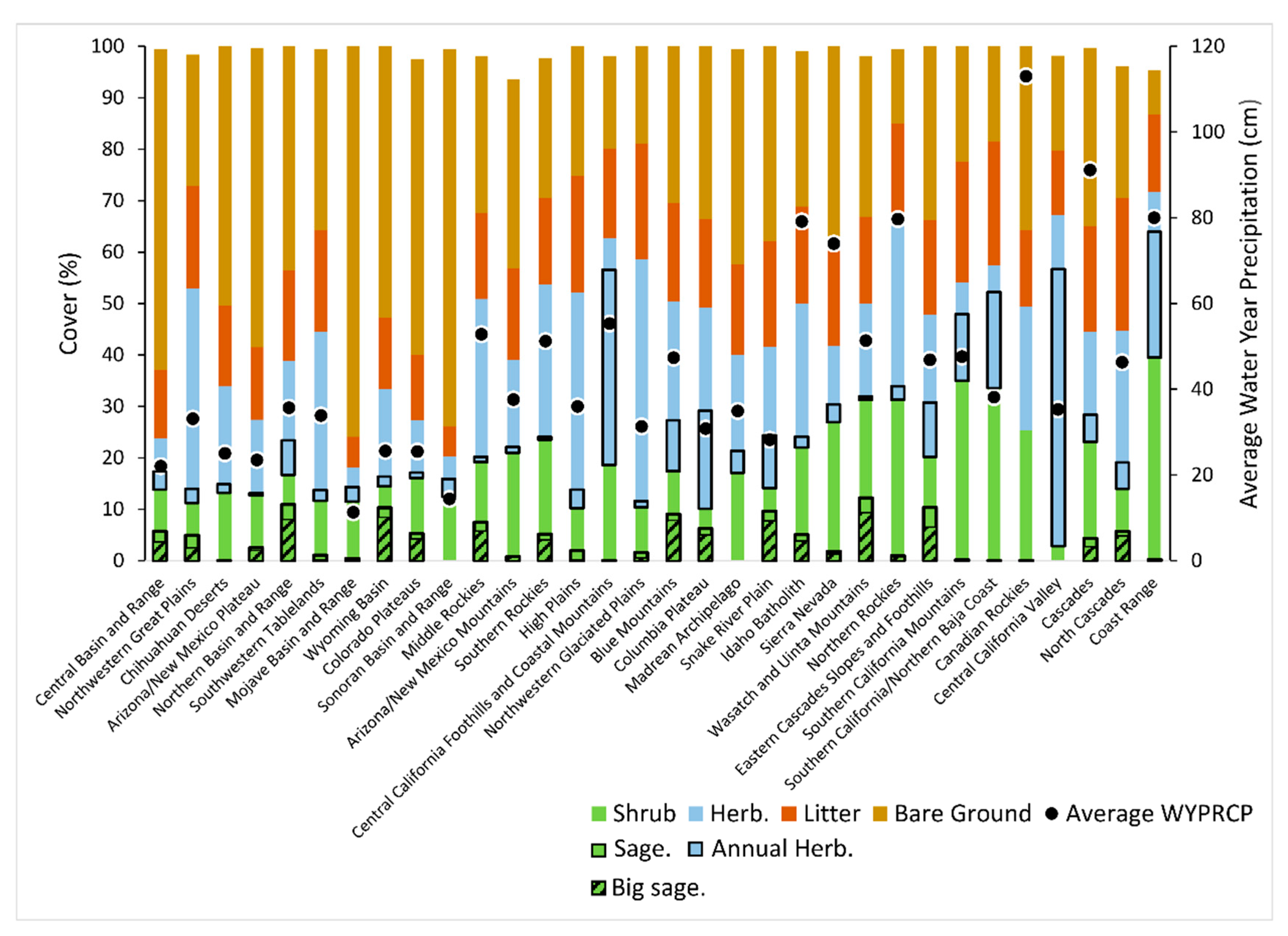
3.3. Ecoregion Averages

Fractional component composition varies widely when summarized by EPA level III ecoregion (Figure 6, Figure S1). Herbaceous cover is highest in the grassland ecoregions: Central California Valley (64.3%) Northwestern Glaciated Plains (48.1%), Central California Foothills, Coastal Mountains (44.0%), and High Plains (41.9%). Annual herbaceous cover is greatest in the northwest and western ecoregions, especially the Central California Valley (54.0%), Central California Foothills and Coastal Mountains (38.1%), Coast Range (24.5%), and Columbia Plateau (19.2%). The Mojave Basin and Range has the highest bare ground (76.4%), while the Coast Range has the lowest (8.6%). Shrub cover tends to be greatest in the mountain ecoregions and in chaparral dominant ecoregions; Coast Range (39.7%), Southern California Mountains (35.1%), Southern California/Northern Baja Coast (33.7%), and Wasatch and Uinta Mountains (31.4%). Conversely, shrub cover averages ~10% in eastern grassland ecoregions. Sagebrush cover patterns are more complex than shrub overall, and weakly related to precipitation. Instead sagebrush cover patterns are primarily driven by temperature, with a strong, negative, relationship with yearly averaged minimum temperature (R2 = 0.40, p < 0.05). Bare ground has the greatest fractional cover among primary components in 17, herbaceous in 11, and shrub in four of the 32 EPA level III ecoregions (Figure 6).

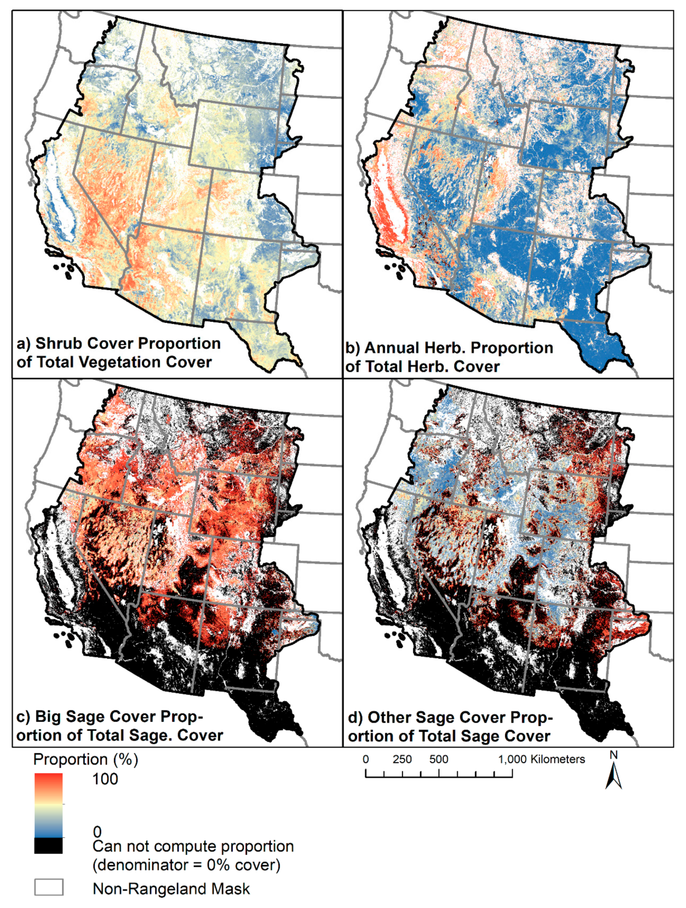
3.4. Component Proportions

Spatial patterns of the secondary components annual herbaceous and big sagebrush are more readily interpreted when viewed as a proportion of their primary component (Figure 7). Shrub cover comprises an average of 40% of total rangeland vegetation cover (shrub plus herbaceous cover) across the study area (Figure 7A). Shrub cover proportion tends to be greatest in the more arid parts of the study area, especially in the Mojave and Sonoran Deserts and Central Basin and Range, and in the California chaparral. Annual herbaceous vegetation is present in 30.1% of the study area, with an average cover of 4.2%, comprising 18.1% of total herbaceous cover (Figure 7B). Annual herbaceous proportion of total herbaceous cover is greatest west of the Sierras in California. Portions of the Mojave and Sonoran Deserts, Snake River Plain, Wasatch Mountains, and Central Basin and Range also have high annual herbaceous proportions.
Sagebrush cover over the study area averages 4.3%, big sagebrush 2.9%, and other sagebrush 1.4% In terms of spatial extent, sagebrush, big sagebrush, and other sagebrush occurs on 41.5%, 35.7%, and 28.8% of the study area, respectively. Within their respective ranges, average sagebrush, big sagebrush, and other sagebrush cover is 10.3%, 8.4%, and 4.4%, respectively. Of pixels with sagebrush present, big sagebrush and other sagebrush co-exist on 55.9% of pixels. Big sagebrush is the predominate sagebrush type in most of the study area (Figure 7C). Other sagebrush is most abundant in the margins of the sagebrush range, especially in the Northwestern Great Plains and Southwest Tablelands ecoregions (Figure 7D).

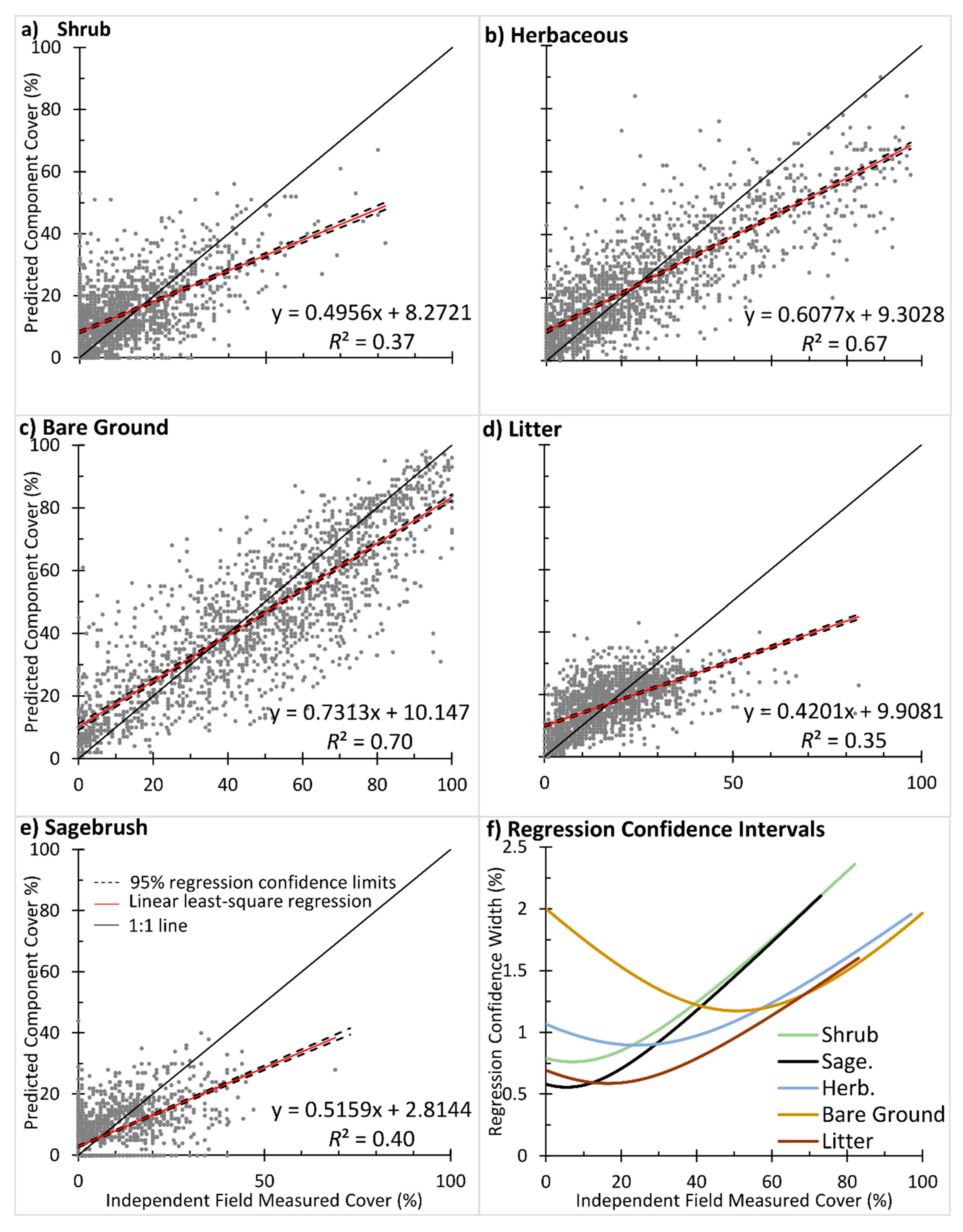
3.5. Component Accuracy

We conducted accuracy assessments of each component prediction using both independent and cross-validation approaches. Table 2a and Figure 8 demonstrate the independent validation results, pooling across regions. Across the cover components, R2 values averaged 0.46, while the average RMSE was 10.37 and the nRMSE was 0.12. Since the range and skewness vary among components (Figure 5), R2 and RMSE need to be considered together in interpreting model performance. Slope is another critical metric; in our case a slope near 1 is preferred as it demonstrates a more unbiased model. Considering all metrics, herbaceous cover and bare ground tended to be the best performers (R2 = 0.67 and 0.70; slope = 0.61 and 0.73, respectively) while shrub height and sagebrush height results had lower accuracies (R2 = 0.19 and 0.24; slope = 0.29 and 0.31, respectively). The width of 95% regression confidence intervals is somewhat related to component histograms, as inferred by box plots (Figure 5), where proximity to the mean component value is related to tighter confidence limits (Figure 8f). Conversely, less common values tend to have broader confidence limits. From a broad scale, however, regression confidence limits do not meaningfully vary across the range of component values.
For the cross-validation assessment (Table 2b), we area-weighted 840,000 data points across all 21 regions according to the proportional contribution of each region to the total mapped area. Patterns were like those of independent validation in terms of relative performance of components and regions, though the accuracies were substantially greater than the independent validation. Like the independent validation, herbaceous cover and bare ground tended to be the best performers in cross-validation (R2 = 0.79 and 0.85; RMSE = 6.3 and 8.0, respectively) while shrub height and sagebrush height results had lower accuracies (R2 = 0.62 and 0.59; RMSE = 17.8 and 7.8 respectively). Across cover components, the average R2 value was 0.69, and the RMSE was 6.8.

4. Discussion

4.1. Component Accuracy

Our mapping approach focused on combining extensive field data (Figure 1), HRS imagery, robust modeling, Landsat imagery from critical phenological periods, and relevant ancillary data into a fractional product designed to retain as much local relevancy as possible, while still being regionally consistent. Validation accuracy results were generally equal to or greater than our previous mapping work [36,39], despite covering much larger geographies. For example, similar fractional component mapping in Wyoming [36] across the five main components (shrub, sagebrush, herbaceous, bare ground, and litter) averaged an R2 of 0.29. Our independent validation results for the same components have an average R2 of 0.54 for Wyoming and R2 of 0.50 across the entire study area (Table 2a). Similarly, Xian et al. [39] demonstrated an average independent validation accuracy of R2 of 0.38 across the same five components, again less robust than found in the present study. However, Xian et al., [39] reported lower RMSE results with an average of 7.49 versus the 10.6 reported here (Table 2a), likely attributed to a larger dynamic range of values in our study area. Relative to independent validation results of fractional component maps developed across the western U.S. by Jones et al. [40] our results show higher accuracy. Of the four components (shrub, bare ground, perennial herbaceous, and annual herbaceous) with independent accuracy reported by Jones et al. [40] the mean R2 was 0.22, verus 0.58 for our equivalent products. Predicted values near the mean of each component tend to be more accurate, but variation in accuracy is minimal across the range of each component (Figure 8). Cross-validation accuracies of our components were substantially better than independent validation results, averaging an R2 of 0.69 and an RMSE of 6.8 across the seven cover components (Table 2b). Our cross-validation results also represent a substantial improvement over the same five components reported in Xian et al. [39].
In judging the product, users should consider both independent and cross-validation accuracy together, since the combination of both provides a more realistic understanding of the performance the user can expect. Cross-validation statistics approximately represent the “best-case” component accuracy, while independent statistics reflect more typical accuracy. One must consider the spatial rate of decay in mapping accuracy between training sites and independent validation sites in interpreting overall accuracy. In other words, consider that the spectral and ecological similarity of a pixel decreases, on average, with distance from training pixels, which /’is related to decreasing environmental similarity with distance [60] in factors such as climate, land use, geology, and species assemblies. We strived to limit spatial decay in accuracy by broadly distributing training data in ecologically and spectrally diverse locations, and by placing Landsat-scale training points in critical locations (Figure 1). The spatial rate of decay tends to be proportionally greatest on shrub, big sagebrush, shrub height, and sagebrush height, which are the most difficult targets to map. Errors do exist in our fractional components as rangelands pose numerous difficulties to mapping, resulting from their high degree of spatial and temporal variation, high amount of bare soil and senescent vegetation [34], and variation in the physical and chemical properties of soils. Errors related to modeling are also present, chief among these is the tendency of component predictions to have a flattened histogram relative to training data.
Height components tend to be the most prone to error (Table 2, [39]), and so users should proceed with caution. Because multispectral data often contain insufficient information to predict canopy height, many researchers have augmented spectral data with light detection and ranging (lidar) data to increase accuracy (e.g., [61]). Lidar data are not yet available at the scale of our study area: even so, we retain our shrub and sagebrush height predictions as they are critical in many rangeland applications such as fire fuel modeling and determining and modeling sage grouse habitat [28,62].
Our mapping region approach was important to localize the prediction and allow customization of each regional model to local conditions. Edge matching of adjacent mapping region was typically quite seamless, suggesting robust modeling that was independently replicating the same component cover in adjacent regions with different models. Methodological improvements did occur as regions were completed. We completed western regions first and then made additional methodological improvements as new issues were encountered in eastern regions. Our advancements relative to Xian et al. [39] included (1) the use of improved handheld tablets in the field to display high-resolution imagery for better plot location and interpretation, (2) sub-meter accuracy GPS units to increase field locational positioning, (3) collecting more plot data on HRS imagery, (4) increasing ground plot supplementation of Landsat-scale training data, and (5) increased experience and consistency of field collection and modeling staff. Regional independent and cross-validation statistics revealed that these improvements yielded higher accuracy numbers even though these regions were generally a more difficult mapping environment primarily because of the higher herbaceous cover which often confounded the spectral signature of shrubs.

4.2. Component Distributions

Component prediction abundance in general follows latitude, longitude, precipitation, and elevation trends (Figure 3 and Figure 4). Northern, eastern and high elevation ecoregions of our study area generally represent the more mesic portions of the landscape (Figure 6). As moisture availability increases in these mesic areas, higher proportions of shrub, herbaceous and litter and lower proportions of bare ground result (Figure 3, Figure 6). Herbaceous vegetation comprises 60% of total rangeland vegetation cover in the study area, with 18.1% of that being annual herbaceous vegetation. The highest proportions of annual herbaceous occur in the western portion of the region, especially in California where invasive annual grasses have supplanted native perennial bunch grasses [9,63]. Significant concentrations of annual herbaceous cover also occur in the Central and Northern Basin and Range, Blue Mountains and Columbia Plateau ecoregions (Figure 4 and Figure 7), where a positive feedback between cheatgrass and fire has altered sagebrush steppe [24,25].
Shrub vegetation comprises 40% of total vegetation cover in the study area, averaging 15.2% cover (Figure 3 and Figure 5). Shrub cover is greatest in the mountain ecoregions, where it is mainly composed of non-sagebrush shrubs such as manzanita (Arctostaphylos spp,), mountain mahogany (Cercocarpus spp.), shrub maples (e.g., Acer grandidentatum), and shrub oaks (e.g., Quercus gambelii). Sagebrush occurs on 41.5% of pixels, mostly across the north central two-thirds of the study area (Figure 4). Big sagebrush habitats, critical to many species including sage grouse [26], though reduced from its historical range [15,29,59] is still widespread (Figure 7C). Other sagebrush cover, particularly silver sagebrush, is also regionally important sage grouse habitat [64]. The concentration of other sagebrush in the Northwestern Great Plains ecoregion is composed mainly of silver sage, while the concentration in the Southwest Tablelands ecoregion is predominately sand sagebrush (Artemisia filifolia) (Figure 7D). Our near range-wide distribution map of sagebrush is similar to that of previously published maps (e.g., [27,65,66]). The additional information presented on our fractional sagebrush cover map versus presence/absence distribution is invaluable to resource managers [29,30].
Litter covers 15.8% of the study area and is most abundant in more mesic areas as a result if th occurrence of more dead plant material in general (Figure 3). More explicitly, litter cover is strongly related to herbaceous cover (R2 = 0.24, p< 0.05). Bare ground occupies the greatest amount of the study area, with an average of 45.5% cover (Figure 5) with the highest proportions in the southern xeric parts of our study area, especially in the Mojave and Sonoran Basin and Range (Figure 3 and Figure 6). Bare ground is the component with the highest mapping accuracy (Table 2a,b); this feature combined with its usefulness as an important indicator of vegetative abundance and rangeland health make it especially useful [67,68]. Relative to an analysis completed by Karl et al. [69] on rangelands managed by the BLM, our study indicated higher amounts of bare ground (Figure 3 and Figure 5). This difference may be attributed to a variety of factors such as different methods of field data collection, different ground targets included as bare ground, and relatively lower sample size in Karl et al. [69]. Additionally, our models tend to over-predict bare ground at the low end of its distribution.

4.3. Next-Generation Work

Accurate characterization of the rangeland landscape is essential to successful understanding of how to manage, monitor and study rangeland processes. Our fractional components provide flexible and accurate remote-sensing-derived products that offer flexible application utility and further enable rangeland monitoring [36]. With this characterization baseline now established, next-generation work is quantifying component change back in time to 1984 using the Landsat archive and analyzing change trends across time [70,71]. Further work is developing site potential and accompanying departure scores to understand where current component predictions have deviated from the expected component amounts based on site condition [72]. Finally, future annual monitoring is underway to quantify how these components are changing. Understanding changing trend rates on the landscape and associated change drivers of those trends will ultimately allow prediction of future change events showing where the landscape is most vulnerable. We also strive to improve fractional component mapping accuracy of all components, particularly shrub and sagebrush height and big sagebrush cover. We are currently testing the usage of 20 m Sentinel imagery with several red edge bands to improve mapping accuracy. Integrating training data from lidar sources could improve the accuracy of height components [61].

5. Conclusions

Our approach for inventorying and quantifying western U.S. rangeland ecosystems as fractional components with remote sensing provides a new way to characterize and monitor these changing regions. Nine rangeland ecosystem components, including percent shrub, sagebrush, big sagebrush, herbaceous, annual herbaceous, litter, and bare ground cover, along with sagebrush and shrub heights in centimeters, were quantified at 30 m resolution across most of the western U.S. using independent mapping regions. Component prediction abundance in general followed latitude, longitude and elevation trends, with the more mesic northern, eastern and high elevation regions of our study area having significantly more shrub, herbaceous and litter amounts, and much less bare ground. Validation accuracy results were generally equal to and in some cases greater than our previous mapping work despite covering much larger geographies. Component composition strongly varies by EPA level III ecoregions, where most ecoregions are bare ground dominant, a minority are herbaceous dominant, and only one is shrub dominant. Sagebrush physically covers 90,950 km², or 4.3%, of our study area, but is present in 883,449 km², or 41.5%, of the non-masked area of our study area, underscoring its widespread distribution. Our near range-wide distribution map of sagebrush is like that of previously published maps. Component products detailed in this paper can be downloaded from www.mrlc.gov.

Supplementary Materials

The following are available online at https://www.mdpi.com/2072-4292/12/3/412/s1, Figure S1. Level III ecoregions boundaries across the study area and Table S1. Description of the fractional cover and height components used to characterize western U.S. rangelands.

Author Contributions

M.R., C.H., H.S., G.X., and M.B. conceptualized the research. M.R. and C.H. wrote the paper. M.R. conducted data analysis and designed the graphics. D.K.M., B.B., H.S., and M.R. prepared the data and ran models. M.R., C.H., L.C., and S.S. collected the field data. All authors have read and agreed to the published version of the manuscript.

Funding

This research was funded by the USGS and BLM under grant L15PG00136.

Acknowledgments

We thank Bruce Wylie, David Pilliod, and anonymous reviewers for reviewing this manuscript. Matthew Rigge and Hua Shi’s work was performed under USGS contracts G13PC00028 and 140G0119C0001. Debbie Meyer and Brett Bunde’s work was performed under USGS contract G15PC00012. Any use of any trade, firm, or product names is for descriptive purposes only and does not imply endorsement by the U.S. Government. Fractional component maps are available at www.mrlc.gov.

Conflicts of Interest

The authors declare no conflict of interest. The funders had no role in the design of the study; in the collection, analyses, or interpretation of data; in the writing of the manuscript, or in the decision to publish the results.

References

  1. Wessel, W.; Tietema, A.; Beier, C.; Emmett, B.A.; Peñuelas, J.; Riis–Nielsen, T. A qualitative ecosystem assessment for different shrublands in western Europe under impact of climate change. Ecosystems 2004, 7, 662–671. [Google Scholar] [CrossRef]
  2. Feld, C.K.; Martins da Silva, P.; Paulo Sousa, J.; De Bello, F.; Bugter, R.; Grandin, U.; Hering, D.; Lavorel, S.; Mountford, O.; Pardo, I.; et al. Indicators of biodiversity and ecosystem services: A synthesis across ecosystems and spatial scales. Oikos 2009, 118, 1862–1871. [Google Scholar] [CrossRef]
  3. Schlesinger, W.H.; Pilmanis, A.M. Plant-soil interactions in deserts. Biogeochemistry 1998, 42, 169–187. [Google Scholar] [CrossRef]
  4. Wallace, O.C.; Qi, J.; Heilma, P.; Marsett, R.C. Remote sensing for cover change assessment in southeast Arizona. J. Range Manag. 2003, 56, 402–409. [Google Scholar] [CrossRef]
  5. Schwinning, S.; Starr, B.I.; Ehleringer, J.R. Summer and winter drought in a cold desert ecosystem (Colorado Plateau) part II: Effects on plant carbon assimilation and growth. J. Arid Environ. 2005, 61, 61–78. [Google Scholar] [CrossRef]
  6. Leu, M.; Hanser, S.E.; Knick, S.T. The human footprint in the west: A large-scale analysis of anthropogenic impacts. Ecol. Appl. 2008, 18, 1119–1139. [Google Scholar] [CrossRef]
  7. Hamada, Y.; Stow, D.A.; Roberts, D.A.; Franklin, J.; Kyriakidis, C. Assessing and monitoring semi-arid shrublands using object-based image analysis and multiple endmember spectral mixture analysis. Environ. Monit. Assess. 2013, 185, 3173–3190. [Google Scholar] [CrossRef]
  8. McKell, C.M.; Garcia-Moya, E. North American Shrub Lands. In The Biology and Utilization of Shrubs; McKell, C.M., Ed.; Academic Press Inc.: San Diego, CA, USA, 1989; 656p. [Google Scholar]
  9. Mack, R.N. Temperate grasslands vulnerable to plant invasions: Characteristics and consequences. In Biological Invasions: A Global Perspective; Drake, J.A., Mooney, H.A., Di Castri, F., Eds.; Wiley: Chichester, UK, 1989; pp. 155–179. [Google Scholar]
  10. Schroeder, M.A.; Aldridge, C.L.; Apa, A.D.; Bohne, J.R.; Braun, C.E.; Bunnell, S.D.; Connelly, J.W.; Diebert, P.A.; Gardner, S.C.; Hilliard, M.A.; et al. Distribution of sage-grouse in North America. Condor 2004, 106, 363–376. [Google Scholar] [CrossRef]
  11. Brown, J.H.; Valone, T.J.; Curtin, C.G. Reorganization of an arid ecosystem in response to recent climate change. Proc. Natl. Acad. Sci. USA 1997, 94, 9729–9733. [Google Scholar] [CrossRef] [Green Version]
  12. Berlow, E.L.; D’Antonio, C.M.; Reynolds, S.A. Shrub expansion in montane meadows: The interaction of local-scale disturbance and site aridity. Ecol. Appl. 2002, 12, 1103–1118. [Google Scholar] [CrossRef]
  13. Knick, S.T.; Dobkin, D.S.; Rotenberry, J.T.; Schroeder, M.A.; Vander Haegen, W.M.; Van Riper, C., III. Teetering on the edge or too late? Conservation and research issues for avifauna of sagebrush habitats. Condor 2003, 105, 611–634. [Google Scholar] [CrossRef]
  14. Bradley, B.A.; Houghton, R.A.; Mustard, J.F.; Hamburg, S.P. Invasive grass reduces aboveground carbon stocks in shrublands of the Western US. Glob. Chang. Biol. 2006, 12, 1815–1822. [Google Scholar] [CrossRef] [Green Version]
  15. Davies, K.W.; Boyd, C.S.; Beck, J.K.; Bates, J.D.; Svejcar, T.J.; Gregg, M.A. Saving the sagebrush sea: An ecosystem conservation plan for big sagebrush plant communities. Biol. Conserv. 2011, 144, 2573–2584. [Google Scholar] [CrossRef] [Green Version]
  16. Walston, L.J.; Cantwell, B.L.; Krummel, J.R. Quantifying spatiotemporal changes in a sagebrush ecosystem in relation to energy development. Ecography 2009, 32, 943–952. [Google Scholar] [CrossRef]
  17. Green, A.W.; Aldridge, C.L.; O’Donnell, M.S. Investigating impacts of oil and gas development on greater sage-grouse. J. Wildl. Manag. 2017, 81, 46–57. [Google Scholar] [CrossRef]
  18. Branson, F.A.; Miller, R.F.; McQueen, I.S. Geographic distribution and factors affecting the distribution of salt desert shrubs in the United States. J. Range Manag. 1967, 20, 287–296. [Google Scholar] [CrossRef]
  19. Cook, J.G.; Irwin, L.L. Climate-vegetation Relationships between the Great Plains and Great Basin. Am. Midl. Nat. 1992, 127, 316–326. [Google Scholar] [CrossRef]
  20. Anderson, J.E.; Inouye, R.S. Landscape scale changes in plant species abundance and biodiversity of the sagebrush steppe over 45 Years. Ecol. Monogr. 2001, 71, 531–556. [Google Scholar] [CrossRef]
  21. Weltzin, J.F.; Loik, M.E.; Schwinning, S.; Williams, D.G.; Fay, P.; Haddad, B.; Harte, J.; Huxman, T.E.; Knapp, A.K.; Lin, G.; et al. Assessing the response of ecological systems to potential changes in precipitation. Bioscience 2003, 53, 941–952. [Google Scholar] [CrossRef]
  22. Xian, G.; Homer, C.; Aldridge, C. Effects of land cover and regional climate variations on long-term spatiotemporal changes in sagebrush ecosystems. GISci. Remote Sens. 2012, 49, 378–396. [Google Scholar] [CrossRef]
  23. Homer, C.; Xian, G.; Aldridge, C.; Meyer, D.; Loveland, T.; O’Donnell, M. Forecasting sagebrush ecosystem components and greater sage-grouse habitat for 2050: Learning from past climate patterns and Landsat imagery to predict the future. Ecol. Indic. 2015, 55, 131–145. [Google Scholar] [CrossRef] [Green Version]
  24. Chambers, J.C.; Bradley, B.A.; Brown, C.S.; D’Antonio, C.; Germino, M.J.; Grace, J.B.; Hardegree, S.P.; Miller, R.F.; Pyke, D.A. Resilience to stress and disturbance, and resistance to Bromus tectorum L. invasion in cold desert shrublands of western North America. Ecosystems 2014, 17, 360–375. [Google Scholar] [CrossRef]
  25. Boyte, S.P.; Wylie, B.K.; Major, D.J. Cheatgrass percent cover change—Comparing recent estimates to climate change–driven predictions in the northern Great Basin. Rangel. Ecol. Manag. 2016, 69, 265–279. [Google Scholar] [CrossRef]
  26. Suring, L.H.; Rowland, M.M.; Wisdom, M.J. Identifying species of conservation concern. In Habitat Threats in the Sagebrush Ecosystem—Methods of Regional Assessment and Applications in the Great Basin; Wisdom, M.J., Rowland, M.M., Suring, L.H., Eds.; Alliance Communications Group: Lawrence, KS, USA, 2005; pp. 150–162. [Google Scholar]
  27. Connelly, J.W.; Knick, S.T.; Schroeder, M.A.; Stiver, S.J. Conservation Assessment of Greater Sage-Grouse and Sagebrush Habitats; Unpublished Report; Western Association of Fish and Wildlife Agencies: Boise, ID, USA, 2004. [Google Scholar]
  28. Aldridge, C.L.; Nielsen, S.E.; Beyer, H.L.; Boyce, M.S.; Connelly, J.W.; Knick, S.T.; Schroeder, M.A. Range-wide patterns of greater sage-grouse persistence. Divers. Distrib. 2008, 14, 983–994. [Google Scholar] [CrossRef] [Green Version]
  29. Miller, R.F.; Knick, S.T.; Pyke, D.A.; Meinke, C.W.; Hanser, S.E.; Wisdom, M.J.; Hild, A.L. Characteristics of sagebrush habitats and limitations to long-term conservation. Stud. Avian Biol. 2011, 38, 145–184. [Google Scholar]
  30. Sant, E.D.; Simonds, G.E.; Ramsey, R.D.; Larsen, R.T. Assessment of sagebrush cover using remote sensing at multiple spatial and temporal scales. Ecol. Indic. 2014, 43, 297–305. [Google Scholar] [CrossRef]
  31. Scott, J.M.; Davis, F.; Csuti, B.; Noss, R.; Butterfield, B.; Groves, G.; Anderson, H.; Caicco, S.; D’Erchia, F.; Edwards, T.C.; et al. Gap analysis: A geographic approach to protection of biological diversity. Wildl. Monogr. 1993, 123, 3–41. [Google Scholar]
  32. Homer, C.G.; Dewitz, J.; Yang, L.; Jin, S.; Danielson, P.; Xian, G.; Coulston, J.; Herold, N.; Wickham, J.; Megown, K. Completion of the 2011 National Land Cover Database for the conterminous United States – representing a decade of land cover change information. Photogramm. Eng. Remote Sens. 2015, 81, 345–353. [Google Scholar]
  33. Rollins, M.G. LANDFIRE: A nationally consistent vegetation, wildland fire, and fuel assessment. Int. J. Wildland Fire 2009, 18, 235–249. [Google Scholar] [CrossRef] [Green Version]
  34. Hagen, S.C.; Heilman, P.; Marsett, R.; Torbick, N.; Salas, W.; van Ravensway, J.; Qi, J. Mapping total vegetation cover across western rangelands with moderate-resolution imaging spectroradiometer data. Rangel. Ecol. Manag. 2012, 65, 456–467. [Google Scholar] [CrossRef]
  35. Sivanpillai, R.; Prager, S.D.; Storey, T.O. Estimating sagebrush cover in semi-arid environments using Landsat thematic mapper data. Int. J. Appl. Earth Obs. Geoinf. 2009, 11, 103–107. [Google Scholar] [CrossRef]
  36. Homer, C.G.; Aldridge, C.L.; Meyer, D.K.; Schell, S. Multi-scale remote sensing sagebrush characterization with regression trees over Wyoming, USA: Laying a foundation for monitoring. Int. J. Appl. Earth Obs. Geoinf. 2012, 14, 233–244. [Google Scholar] [CrossRef]
  37. Sivanpillai, R.; Ewers, B.E. Relationship between sagebrush species and structural characteristics and Landsat thematic mapper data. Appl. Veg. Sci. 2013, 16, 122–130. [Google Scholar] [CrossRef]
  38. Xian, G.; Homer, C.; Meyer, D.; Granneman, B. An approach for characterizing the distribution of shrubland ecosystem components as continuous fields as part of NLCD. ISPRS J. Photogramm. Remote Sens. 2013, 86, 136–149. [Google Scholar] [CrossRef]
  39. Xian, G.; Homer, C.; Rigge, M.; Shi, H.; Meyer, D. Characterization of shrubland ecosystem components as continuous fields in the northwest United States. Remote Sens. Environ. 2015, 168, 286–300. [Google Scholar] [CrossRef] [Green Version]
  40. Jones, M.O.; Allred, B.W.; Naugle, D.E.; Maestas, J.D.; Donnelly, P.; Metz, L.J.; Karl, J.; Smith, R.; Bestelmeyer, B.; Boyd, C.; et al. Innovation in rangeland monitoring: Annual, 30 m, plant functional type percent cover maps for U.S. rangelands, 1984–2017. Ecosphere 2018, 9, e02430. [Google Scholar] [CrossRef]
  41. Omernik, J.M.; Griffith, G.E. Ecoregions of the conterminous United States: Evolution of a hierarchical spatial framework. Environ. Manag. 2014, 54, 1249–1266. [Google Scholar] [CrossRef]
  42. USDA; NRCS. The PLANTS Database; National Plant Data Team: Greensboro, NC, USA, 2019. Available online: http://plants.usda.gov (accessed on 24 April 2019).
  43. Yang, L.; Jin, S.; Danielson, P.; Homer, C.; Gass, L.; Bender, S.M.; Case, A.; Costello, C.; Dewitz, J.; Fry, J.; et al. A new generation of the United States National Land Cover Database: Requirements, research priorities, design, and implementation strategies. ISPRS J. Photogramm. Remote Sens. 2018, 146, 108–123. [Google Scholar] [CrossRef]
  44. Assessment, Inventory, and Monitoring (AIM). Available online: https://landscape.blm.gov/geoportal/catalog/AIM/AIM.page (accessed on 5 September 2018).
  45. RuleQuest Research. Cubist; Version 2.08; RuleQuest Pty: St. Ives, New South Wales, Australia, 2008. [Google Scholar]
  46. Wylie, B.; Pastick, N.; Picotte, J.; Deering, C. Geospatial data mining for digital raster mapping. GISci. Remote Sens. 2019, 56, 406–429. [Google Scholar] [CrossRef]
  47. Jenkerson, C.B.; Maiersperger, T.K.; Schmidt, G.L. eMODIS: A User-Friendly Data Source; U.S. Geological Survey Open-File Report; USGS: Reston, VA, USA, 2010. Available online: https://doi.org/10.3133/ofr20101055 (accessed on 13 November 2017).
  48. Chander, G.; Huang, C.; Yang, L.; Homer, C.; Larson, C. Developing consistent Landsat data sets for large area applications: The MRLC 2001 protocol. IEEE Geosci. Remote Sens. Lett. 2009, 6, 777–781. [Google Scholar] [CrossRef]
  49. Jenkerson, C. User Guide: Earth Resources Observation and Science (EROS) Center Science Processing Architecture (ESPA) on Demand Interface, 1.4 ed.; U.S. Geological Survey: Reston, VA, USA, 2013.
  50. Schmidt, G.; Jenkerson, C.B.; Masek, J.; Vermote, E.; Gao, F. Landsat Ecosystem Disturbance Adaptive Processing System (LEDAPS) Algorithm Description. In U.S. Geological Survey Open-File Report; USGS: Reston, VA, USA, 2013. Available online: https://doi.org/10.3133/ofr20131057 (accessed on 7 July 2017).
  51. Boyte, S.P.; Wylie, B.K.; Rigge, M.B.; Dahal, D. Fusing MODIS with Landsat 8 data to downscale weekly normalized difference vegetation index estimates for central Great Basin rangelands, USA. GISci. Remote Sens. 2018, 55, 376–399. [Google Scholar] [CrossRef]
  52. Gao, F.; Masek, J.; Schwaller, M.; Hall, F. On the blending of the Landsat and MODIS surface reflectance: Predicting daily Landsat surface reflectance. IEEE Trans. Geosci. Remote Sens. 2006, 44, 2207–2218. [Google Scholar]
  53. Chambers, J.C.; Beck, J.L.; Campbell, S.; Carlson, J.; Christiansen, T.J.; Clause, K.; Dinkins, J.B.; Doherty, K.E.; Griffin, K.A.; Havlina, D.W.; et al. Using resilience and resistance concepts to manage threats to sagebrush ecosystems, Gunnison sage-grouse, and greater sage-grouse in their eastern range. In General Technical Report RMRS-GTR-356; Department of Agriculture, Forest Service, Rocky Mountain Research Station: Fort Collins, CO, USA, 2016; 143p. [Google Scholar]
  54. Geospatial Mulit-Agency Coordination. Available online: https://www.geomac.gov/ (accessed on 21 May 2016).
  55. Lesica, P.; Cooper, S.V.; Kudray, G. Recovery of big sagebrush following fire in southwest Montana. Rangel. Ecol. Manag. 2007, 60, 261–269. [Google Scholar] [CrossRef]
  56. Beck, J.L.; Connelly, J.W.; Reese, K.P. Recovery of greater sage-grouse habitat features in Wyoming big sagebrush following prescribed fire. Restor. Ecol. 2009, 17, 393–403. [Google Scholar] [CrossRef]
  57. Han, W.; Yang, Z.; Di, L.; Yue, P. A Geospatial Web Service Approach for Creating On-Demand Cropland Data Layer Thematic Maps. Trans. ASABE 2013, 57, 239–247. [Google Scholar]
  58. Thornton, P.E.; Thornton, M.M.; Mayer, B.W.; Wei, Y.; Devarakonda, R.; Vose, R.S.; Cook, R.B. Daymet: Daily Surface Weather Data on a 1-km Grid for NORTH AMERICA, Version 3. 2016. Available online: https://doi.org/10.3334/ORNLDAAC/1328 (accessed on 14 March 2017).
  59. West, N.E.; Young, J.A. Intermountain valleys and lower mountain slopes. In North American Terrestrial Vegetation; Barbour, M.G., Billing, W.D., Eds.; Cambridge University Press: Cambridge, UK, 2000; pp. 255–284. [Google Scholar]
  60. Nekola, J.C.; White, P.S. The distance decay of similarity in biogeography and ecology. J. Biogeogr. 1999, 26, 867–878. [Google Scholar] [CrossRef] [Green Version]
  61. Ku, N.-W.; Popescu, S.C. A comparison of multiple methods for mapping local-scale mesquite tree aboveground biomass with remotely sensed data. Biomass Bioenergy 2019, 122, 270–299. [Google Scholar] [CrossRef]
  62. Smith, J.T.; Tack, J.D.; Berkeley, L.I.; Szczypinski, M.; Naugle, D.E. Effects of livestock grazing on nesting sage-grouse in central Montana. J. Wildl. Manag. 2018, 82, 1503–1515. [Google Scholar] [CrossRef]
  63. Mordecai, E.A.; Molinari, N.A.; Stahlheber, K.A.; Gross, K.; D’Antonio, C. Controls over native perennial grass exclusion and persistence in California grasslands invaded by annuals. Ecology 2015, 96, 2643–2652. [Google Scholar] [CrossRef] [Green Version]
  64. Jones, P.F.; Penniket, R.; Fent, L.; Nicholson, J.; Adams, B. Silver sagebrush community associations in southeastern Alberta, Canada. Rangel. Ecol. Manag. 2005, 58, 400–405. [Google Scholar] [CrossRef]
  65. Shultz, L.M. Monograph of Artemisia Subgenus Tridentatae (Asteraceae–Anthemideae). Syst. Botany Monogr. 2009, 89, 1–131. [Google Scholar]
  66. Chambers, J.C.; Beck, J.L.; Bradford, J.B.; Bybee, J.; Campbell, S.; Carlson, J.; Christiansen, T.J.; Clause, K.J.; Collins, G.; Crist, M.R.; et al. Science basis and applications. Gen. Tech. Rep. RMRS-GTR-360. In Science Framework for Conservation and Restoration of the Sagebrush Biome: Linking the Department of the Interior’s Integrated Rangeland Fire Management Strategy to Long-Term Strategic Conservation Actions. Part 1; Department of Agriculture, Forest Service, Rocky Mountain Research Station: Fort Collins, CO, USA, 2017; 213p. [Google Scholar]
  67. Pyke, D.A.; Herrick, J.E.; Shaver, P.; Pellant, M. Rangeland health attributes and indicators for qualitative assessment. J. Range Manag. 2002, 55, 584–597. [Google Scholar] [CrossRef]
  68. Booth, D.T.; Tueller, P.T. Rangeland monitoring using remote sensing. Arid Land Res. Manag. 2003, 17, 455–467. [Google Scholar] [CrossRef]
  69. Karl, M.G.; Kachergis, E.; Karl, J.W. Bureau of Land Management Rangeland Resource Assessment—2011; U.S. Department of the Interior, Bureau of Land Management, National Operations Center: Denver, CO, USA, 2016; 96p.
  70. Shi, H.; Rigge, M.; Homer, C.G.; Xian, G.; Meyer, D.K.; Bunde, B. Historical cover trends in a sagebrush steppe ecosystem from 1985 to 2013: Links with climate, disturbance, and management. Ecosystems 2018, 21, 913–929. [Google Scholar] [CrossRef]
  71. Rigge, M.; Shi, H.; Homer, C.; Danielson, P.; Granneman, B. Long-term trajectories of fractional component change in the Northern Great Basin. USA Ecosphere 2019, 10, e02762. [Google Scholar] [CrossRef]
  72. Rigge, M.B.; Homer, C.G.; Wylie, B.K.; Gu, Y.; Shi, H.; Xian, G.; Meyer, D.K.; Bunde, B. Using remote sensing to quantify ecosystem site potential community structure and deviation in the Great Basin, United States. Ecol. Indic. 2019, 96, 516–531. [Google Scholar] [CrossRef]
Figure 1. Mapping regions and field data used in model development and assessment of fractional cover components in the western U.S. Mapping region names are indicated by italicized text, and state abbreviations annotated. Inset map shows the nominal year in which field observations and Landsat imagery were obtained for each region.
Remotesensing 12 00412 g001
Figure 2. Overview of major processing steps and data inputs for characterization of rangeland fractional component cover.
Remotesensing 12 00412 g002
Figure 3. Distribution of primary fractional cover components; shrub, herbaceous, bare ground, and litter in the western U.S.
Remotesensing 12 00412 g003
Figure 4. Distribution of secondary fractional cover components; all sagebrush, big sagebrush, and annual herbaceous, and shrub height in cm. Note the color ramps of all sagebrush, big sagebrush, and annual herbaceous have been truncated to a range of 0–50% cover and shrub height truncated to 0–150 cm to enhance visualization.
Remotesensing 12 00412 g004
Figure 5. Box plots of component cover (%)/height (cm). Left box corresponds with the 1st quartile through median, right box is the median through 3rd quartile. Left and right whiskers are minimum and maximum, respectively. Maximum values of shrub and sagebrush height are labeled.
Remotesensing 12 00412 g005
Figure 6. U.S. Environmental Protection Agency (EPA) level III ecoregion average component cover. Color corresponds to the primary components of shrub, herbaceous, litter, and bare ground. Sagebrush and annual herbaceous cover are nested (i.e., secondary) to shrub cover and herbaceous cover, respectively, shown as boxes within their primary component. Big sagebrush is nested within sagebrush and is shown as the hatched box within the secondary sagebrush box. Primary components plus tree cover are designed to sum to 100% Ecoregions are listed in order of decreasing mapped area from left to right. Secondary y-axis shows average water year precipitation (WYPRCP) within the mapped portion of the ecoregion, indicated by black points. See Figure S1 for locations of level III ecoregions.
Remotesensing 12 00412 g006
Figure 7. Fractional cover proportions. (a) shrub cover proportion of total vegetation (shrub + herbaceous) cover, (b) annual herbaceous proportion of herbaceous cover, (c) big sagebrush proportion of sagebrush cover, and (d) other sagebrush (sagebrush – big sagebrush) proportion of sagebrush cover.
Remotesensing 12 00412 g007
Figure 8. Independent accuracy scatterplots (n = 1860) and 95% regression confidence limits for field measured versus predicted cover of selected components: (a) shrub, (b) herbaceous, (c) bare ground, (d) litter, and (e) sagebrush cover. (f) Width of 95% regression confidence limits (upper limits minus.
Remotesensing 12 00412 g008
Table 1. Component distribution statistics. Components are mapped as fractional proportions of each 30 m pixel, with area estimates converted to square kilometers to generate the total area covered by each fractional component. Shrub and sagebrush height area is reflective of their respective parent components of shrub and sagebrush cover. Mapped area reflects the total geography with component predictions. Pixels with component present is the percentage of the mapped area in which component cover is greater than 0% or 0 cm by component.
ComponentArea (km2)Pixels with Component Present (%)
Shrub *324,24795.1
Shrub Height324,24795.1
Sagebrush90,94941.5
Sagebrush Height90,94941.5
Big Sagebrush63,83835.7
Herbaceous *490,51799.5
Annual Herb.89,16530.1
Litter *335,68899.7
Bare Ground *968,79299.9
Non-Rangeland833,836
Mapped Area2,129,819
Total Area2,993,655
* Indicates a primary component, which represents 100% of the mapped area when added together with tree cover.
Table 2. Validation results of component predictions compared to (a) independent field-measured observations (n = 1860) and (b) cross-validation 30 m training data (n = 840,000) used in model development. Cross-validation statistics were area-weighted by mapping region. Units for average, max and range are in percent, except for shrub and sagebrush height (ht), which are in centimeters.
(a) Independent Validation
ShrubSageBig SageHerbAnnual HerbLitterBare GroundShrub HtSage Ht
Average11.85.72.924.06.716.847.344.517.7
Max826969979783100400150
Range826969979783100400150
R20.370.400.160.670.580.350.700.190.24
Slope0.500.520.340.610.550.420.730.290.31
RMSE10.67.57.813.19.88.914.639.525.6
nRMSE0.130.110.110.140.100.110.150.100.19
(b)Cross-Validation
ShrubSageBig SageHerbAnnual HerbLitterBare GroundShrub HtSage Ht
Average15.75.64.122.66.016.344.440.813.3
Max8759591009274100865239
Range8759591009274100865239
R20.730.630.630.790.660.750.850.620.59
Slope0.700.630.620.740.640.710.780.620.59
RMSE6.03.44.16.34.13.88.017.87.8
nRMSE0.070.060.070.060.040.050.080.020.03

