Modelling the Altitude Dependence of the Wet Path Delay for Coastal Altimetry Using 3-D Fields from ERA5

Abstract

Wet path delay (WPD) for satellite altimetry has been provided from external sources, raising the need of converting this value between different altitudes. The only expression available for this purpose considers the same altitude reduction, irrespective of geographic location and time. The focus of this study is the modelling of the WPD altitude dependence, aiming at developing improved expressions. Using ERA5 pressure level fields (2010–2013), WPD vertical profiles were computed globally. At each location and for each vertical profile, an exponential function was fitted using least squares, determining the corresponding decay coefficient. The time evolution of these coefficients reveals regions where they are highly variable, making this modelling more difficult, and regions where an annual signal exists. The output of this modelling consists of a set of so-called University of Porto (UP) coefficients, dependent on geographic location and time. An assessment with ERA5 data (2014) shows that for the location where the Kouba coefficient results in a maximum Root Mean Square (RMS) error of 3.2 cm, using UP coefficients this value is 1.2 cm. Independent comparisons with WPD derived from Global Navigation Satellite Systems and radiosondes show that the use of UP coefficients instead of Kouba’s leads to a decrease in the RMS error larger than 1 cm.

1. Introduction

The presence of water in the atmosphere plays a key role in the Earth’s climate, being crucial for human life. With economic and social impacts, remote sensing techniques have been developed to measure and monitor the water vapor content in the troposphere, namely its vertical distribution [1]. However, the water vapor content in the atmosphere is itself an undesirable factor for some remote sensing techniques, as satellite radar altimetry, whose final purpose is not to measure the atmospheric properties.

Satellite altimetry’s main objective is the measurement of the sea surface height (SSH) above a reference surface [2], allowing applications as the monitoring of the mean sea level [3,4], at global or regional scales. The SSH depends on the measurement of the range between the satellite orbit and the sea surface and on the satellite altitude above the same reference surface. Contrary to what happens in the vacuum, the propagation of the radar signals through the atmosphere is affected by its constituents [5]. One of these effects is the path delay induced by the wet troposphere, which, in the context of satellite altimetry, is one of the atmospheric corrections to be considered: the wet tropospheric correction (WTC). Since this delay leads to an additional path induced by the wet troposphere, the WTC is a negative value in the altimetric equations involved in the SSH estimation. Mainly due to the presence of water vapor in the troposphere, the WTC has a maximum absolute value of 0.5 m. Hereafter, for simplification, its absolute value, the wet path delay (WPD) is adopted.

Accurate determination of SSH from satellite altimetry, either over the ocean or continental waters, depends on the accuracy of all terms involved in its computation, namely the WPD. It is known that the water vapor concentration is highly variable in the atmosphere, both in space and time, and its greatest concentration is near the ground and in the tropics [6]. Due to this complex 4-D variation, for altimetry applications over open-ocean, the WPD is best determined from collocated measurements provided by Microwave Radiometers (MWR), passive instruments on board most of altimetric missions [7]. Satellite altimetry has been used over coastal [8,9,10] and inland waters [5,11], however the WPD retrievals from MWR measurements become invalid and cannot be used over these regions [12]. The current algorithms that compute the WPD from MWR measurements have been tuned to conditions only over ocean surfaces [13]. When different surfaces (e.g., land) are present in the footprint of the MWR, the algorithms will return the corresponding ocean-like WPD, resulting in invalid values over e.g., coastal and continental waters.

Alternative sources to provide valid WPD values for these zones can be the Global Navigation Satellite Systems (GNSS) ground stations [12,14] and Numerical Weather Models (NWM) [5,15], e.g., those from the European Centre for Medium-Range Weather Forecasts (ECMWF). These different WPD sources have been used together in order to develop improved WPD products for satellite altimetry, with significant impacts over coastal zones [16,17,18]. Since these WPD sources are different in terms of spatial coverage, temporal sampling, reference surface and accuracy, appropriate procedures are required to handle the different observations and to retrieve the best WPD estimation [19].

Designed for applications over the ocean, altimetric missions are mainly focused on the sea surface and, for this reason, MWR-derived WPD measurements refer to the sea level. On the contrary, WPD derived from an NWM are computed at the level of its orography (usually a smoothed representation of a digital elevation model), which can depart from the actual surface by hundreds of meters [5]. The path delays derived from GNSS are available at each station height [14], which for some coastal and island stations can be larger than 2000 m. Due to the differences between these three data types (MWR, NWM, and GNSS), namely their reference surfaces, the modelling of the height dependence of the WPD is crucial information to better combine these different WPD sources for altimetry application over coastal and inland waters. Over coastal zones, all measurements must refer to the sea level, while over continental waters they must refer to the level of the corresponding water body. Therefore, an expression to reduce the WPD from GNSS station height and orography level to sea level (over coastal zones) and to water body height (over inland waters) is required.

At present, there is an expression for the altitude reduction of the WPD developed by Kouba [20], however this equation has some limitations due to the complex 4-D variation of the WPD, since it assumes that this altitude dependence is the same over the whole globe.

For real-time applications like aircraft navigation and positioning, similar approaches for the modelling of this height dependence that provide WPD (or equivalent values) without meteorological measurements are used [21,22,23]. As these approaches were not developed for altimetry applications, they have precisions of various centimeters.

The focus of this research is the modelling of the height dependence of the WPD, aiming to derive improved expressions to account for its complex 4-D variation, required for regions of interest, as coastal and continental waters. These expressions are crucial for the retrieval of accurate WPD measurements over the latter regions, such as rivers and lakes, very important for obtaining accurate absolute water levels.

For this modelling, global WPD estimations at vertical profiles are required, which can be obtained from various sources, such as NWM, GNSS tomography, or radiosondes (RS). The RS network is the primary in-situ observing system for monitoring the atmosphere, giving unique information on the distribution and variability of water vapor in the troposphere. RS measurements provide vertical profiles of the meteorological variables required for the WPD retrieval (pressure, temperature, and humidity), as well as the geopotential height. Usually, radiosondes are expected to measure WPD with an uncertainty up to 1.2 cm [24]. However, the use of radiosondes is restricted by their high operational costs, decreasing sensor performance in cold dry conditions, and their poor spatial coverage [25].

GNSS is an operational tool for measuring the atmospheric water vapor, allowing the estimation of WPD at the station height with an accuracy of some millimeters [14]. The advantages of GNSS are that it makes continuous measurements possible and the spatial density of the current GNSS networks is higher than that of the radiosonde network. Concerning the GNSS tomography in which the 3-D water vapor content is estimated, it takes advantage of observing the wet delays in the slant direction. If a network of GNSS stations is available, a vertical discretization of the water vapor content can be achieved. The disadvantage of the GNSS tomography is its spatial coverage (a regional portion of the troposphere, covered by the GNSS network) [26,27].

Only NWM provide global data at a regular temporal sampling. For this reason, WPD vertical profiles computed from NWM were selected. For this purpose, the latest reanalysis model from ECMWF [28], ERA5, was used. This new reanalysis provides hourly atmospheric fields at 0.25° × 0.25° spatial sampling on 137 vertical levels (from the surface up to an altitude around 80 km).

This study is performed in three main steps. First, the errors introduced when applying the Kouba expression globally (using a constant coefficient) are assessed. This provides a quantification of the magnitude of the errors and their spatial distribution. For this, global WPD vertical profiles from ERA5 are computed and analyzed. Exploiting the knowledge acquired in the first step, improved expressions for the vertical variation of the WPD are determined in the second step, from WPD at ERA5 vertical levels, considering regional and temporal dependent coefficients. The last step of this study is an assessment (selecting ERA5 data not used in the modelling) and a validation (using radiosondes and GNSS data). This allows to inspect the significance of this improved modelling in the handling of wet path delays for satellite altimetry in regions such as coastal and inland waters.

Section 2 presents the different data and methodologies adopted in this study, both for the WPD computation and for the modelling of its vertical distribution, while Section 3 presents the results and the discussion of this work. Finally, Section 4 summarizes the main achievements of this research and its impact on the wet tropospheric correction for coastal altimetry.

2. Data and Methods

The modelling described in this paper was performed using global atmospheric variables on vertical levels from ERA5 every 3h, for a time span of 4 years (2010–2013). Data from the same model for a different time span (2014) were used for its assessment. For validation purposes, GNSS and radiosondes data over the year 2014 were used. This section describes these data and the methodologies used to derive WPD from them, both at vertical profiles and at a single vertical level (e.g., GNSS station altitude or ERA5 orography height), as well as the methods used for the modelling of the WPD altitude dependence.

2.1. Data Sources for WPD Estimation

In this section, the computation of WPD from atmospheric fields provided by NWM is described. The same computation is also performed using in-situ atmospheric measurements from radiosondes. The methodology to derive WPD from GNSS data is also addressed. Together with radiosonde measurements, they are used as independent observations to validate the modelling proposed in this paper.

2.1.1. Numerical Weather Models (NWM)

The computation of wet delays from NWM for application in satellite altimetry is commonly performed from products provided by ECMWF, as the operational model with a spatial resolution of 0.125° × 0.125° and temporal sampling of 6h or the ERA Interim reanalysis [29] with the same temporal resolution and a slightly worse spatial sampling (0.75° × 0.75°). ERA Interim is more stable than the ECMWF operational model [15], however the latter has been updated and improved and after 2004 it provides similar or better results than ERA Interim [5]. More recently, ECMWF released the fifth and the latest major global reanalysis ERA5 [28], which is freely available for any user via the Copernicus Climate Change Service (C3S) Climate Data Store (CDS). In this study, the ERA5 reanalysis was adopted.

When compared with its predecessor (ERA Interim), ERA5 has higher spatial (0.25° × 0.25°) and temporal (1h) resolutions and an improved troposphere modelling. It is the first ECMWF model available at 1h intervals. Previous studies [30] show that this new and improved temporal resolution has a small impact in the WPD computation for satellite altimetry, when compared with the common temporal resolution of 6h. As recognized for the previous atmospheric models, ERA5 also cannot map the WPD small space and time scales, evidencing the limitations of the latest ECMWF reanalysis, even with atmospheric variables at 1h intervals [30]. In spite of these limitations, when compared with its predecessor ERA Interim, ERA5 shows a global reduction of the WPD Root Mean Square (RMS) error of 0.2 cm. For some latitude bands, the improvement can reach 0.4 cm, illustrating the considerable impact of the new reanalysis in the computation of radar altimeter wet path delays.

The WPD retrieval from an NWM such as ERA5 can be performed from two types of data: single level (SL) variables provided at surface level and those provided at vertical levels (3-D). The first ones are variables available at a single vertical level (the orography height of the corresponding NWM). Some of these fields are representative of the total atmospheric column (integrated variables). The single level variables are provided at global regular grids and allow the computation of the WPD for the same spatial and temporal resolutions, at the corresponding NWM orography height. WPD values for along-track satellite altimeter observations must be obtained interpolating in space and time the gridded products, further reduced to the height of interest (e.g., sea level or water body height).

The computation from SL variables can be performed from two atmospheric fields—Total Column Water Vapor (TCWV) and two-meter temperature (T₀), according to Equations (1) and (2):

$$WPD=\left[0.101995+\frac{1725.55}{T_m}\right]\frac{TCWV}{1000}.$$

(1)

Equation (1) proposed by [31,32] allows the computation of WPD in meters, using TCWV in kg.m⁻². TCWV is a measure of the total water vapor contained in a vertical column of atmosphere, part of the altimetric signal path. Using the density of water equal to 1000 kg.m⁻³, TCWV is equivalent to the height of a column of water expressed in millimeters (1 kg.m⁻² = 1 mm), designated as precipitable water. Thus, TCWV corresponds to the height the water would occupy if the vapor was condensed into liquid and spread evenly across the column. Typically, with maximum values around 75 kg.m⁻² for low latitudes (or 75 mm of precipitable water), TCWV is related with WPD through the simple relation: WPD = 6.4 × TCWV, with TCWV and WPD in the same length units [19,31]. For the TCWV maximum value of 7.5 cm, the corresponding WPD is around 48 cm. However, this relation is not accurate enough.

The term T_m in Equation (1) is the mean atmospheric temperature, in Kelvin, which can be obtained from the near-surface temperature (T₀), by means of a linear relation according to e.g., Equation (2) proposed by [33].

$$T_m=50.440+0.789 T_0.$$

(2)

In Equations (1) and (2), T₀ and T_m are in Kelvin, TCWV in millimeters and the WTC results in meters. Adopting these two equations, WPD can be derived from an NWM single level variable, the so-called 2-D approach, leading to a less intensive computation. Note that thanks to the use of the integrated TCWV field, the estimated WPD value is representative of the total signal path. The disadvantage of this approach is the fact that it only allows the WPD computation at a single vertical level (the NWM orography height).

The second type of data provided by NWM for WPD computation are the atmospheric variables available at vertical levels (3-D fields). At each grid point, irrespective of its altitude, ERA5 provides atmospheric variables on 137 model levels (ML), from the surface up to 0.01 hPa (around an altitude of 80 km). These variables are also interpolated to standard levels, such as pressure levels (PL), which correspond to 37 levels (1, 2, 3, 5, 7, 10, 20, 30, 50, 70, 100, 125, 150, 175, 200, 225, 250, 300, 350, 400, 450, 500, 550, 600, 650, 700, 750, 775, 800, 825, 850, 875, 900, 925, 950, 975, and 1000 hPa), from an altitude around 45–50 km (1 hPa) down to the surface at 1000 hPa. Unlike model levels, which, for each point, correspond to different pressure values, the pressure levels are always the same, irrespective of the location or the corresponding surface height. For regions where the surface height is above the lowest pressure level, the atmospheric variables for PL below the surface height are extrapolated.

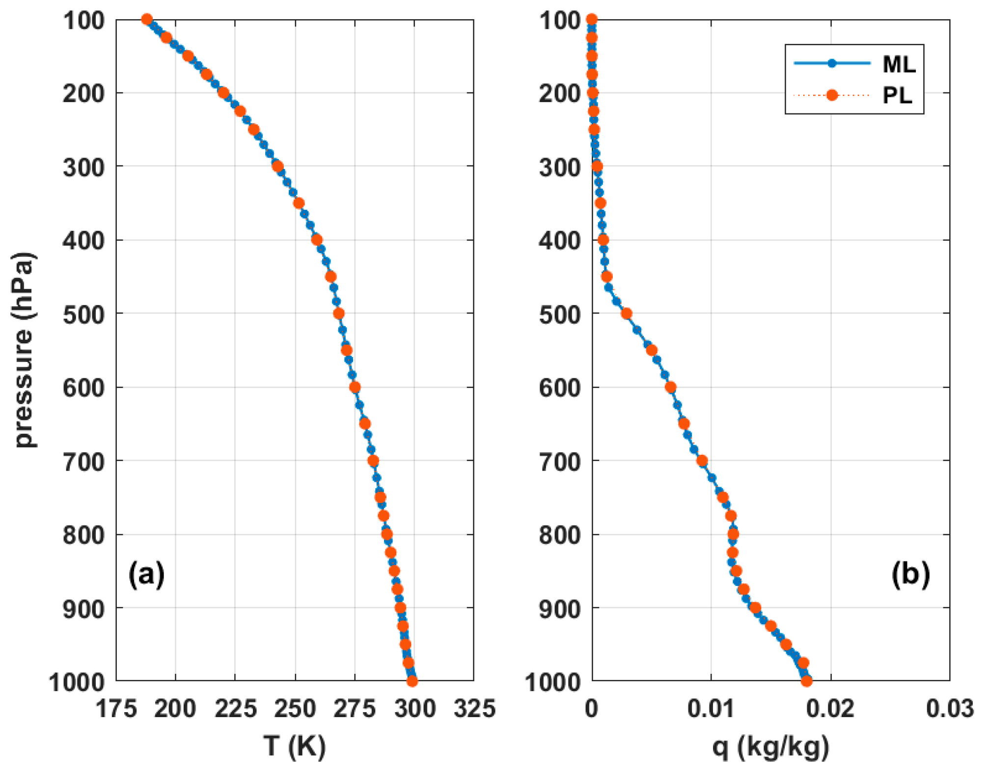
As an example, Figure 1 shows the temperature (T) and the specific humidity (q) at the location with coordinates 00°, 120°E provided by ERA5 on 1 January 2010, at 00:00 UTC. Blue points are the variables provided on model levels (137), while orange points represent the variables on pressure levels (37). Pressure in hPa is represented in the vertical axes, for which the 1000 hPa level is close to the surface, while pressures of 500 and 200 hPa correspond to altitudes around 6 and 12 km, respectively. These values are approximate, since the correspondence between pressure and altitude depends on the geographic location.

Observing Figure 1b, the specific humidity has a complex vertical distribution and becomes negligible for levels above 300–200 hPa (~10 km). On the contrary, Figure 1a shows a linear temperature decrease with altitude up to an height of about 10 km, with a mean temperature lapse rate of −6.5 K/km [34,35]. Figure 1 shows that the pressure levels (orange), even being less (37) than the ML (137), are enough to describe the atmospheric vertical profiles well. These characteristics are common for the entire globe. The results shown in Section 3 demonstrate that the use of PL, instead of ML, provides similar global results, without significant WPD differences. Moreover, the estimations with PL are much more computationally efficient.

The WPD retrieval from these 3-D variables (either on ML or on PL) can be accomplished from a numerical integration of these two variables (temperature and specific humidity), according to Equation (3) [36]. This numerical integration is performed from the level at the top of atmosphere (TOA), with pressure P_TOA, down to the level at surface (with pressure P_surf). In Equation (3), q and T are the specific humidity in kg/kg and the temperature in Kelvin, respectively, $\phi$ is the latitude, the pressures are given in hPa, and the WPD at the lowest (surface) level results in meters.

$$WPD=\left[1.116454\times {10}^{-3}{{\displaystyle \int }}_{P_{TOA}}^{P_{surf}}q dp+17.66543928{{\displaystyle \int }}_{P_{TOA}}^{P_{surf}}\frac{q}{T} dp\right]\times \left[1+0.0026\cos 2\phi \right].$$

(3)

For a less intensive computation, ERA5 data on levels up to 200 hPa (approximately 20 pressure levels) are adequate, since the specific humidity of the upper levels is negligible and the corresponding WPD is null.

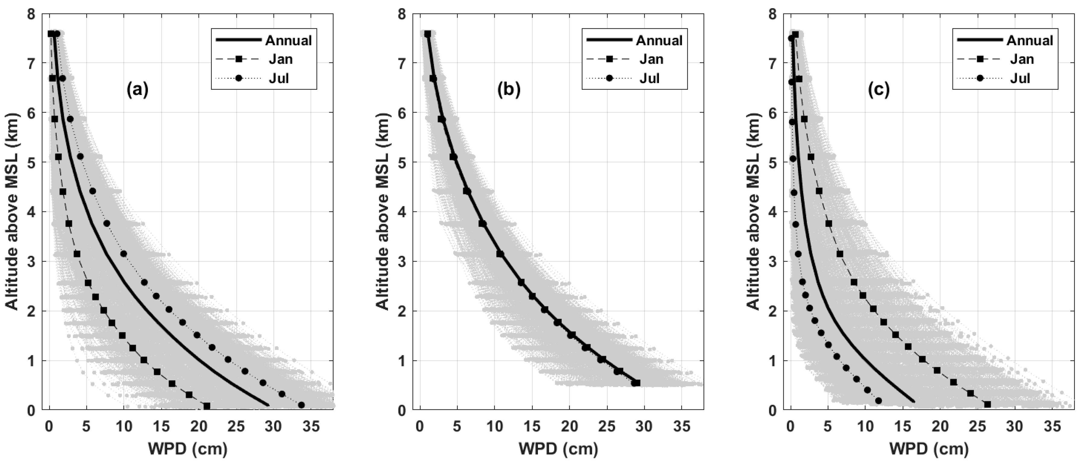
The WPD from the so-called 3-D approach was computed using Equation (3) from ERA5 data on vertical pressure levels in a global grid of 5° × 5°. Figure 2 shows examples of WPD profiles at three different locations (only PL above the surface were considered). Grey points represent all WPD vertical profiles, every 3h, over one complete year (2010) and the solid line represents the corresponding annual mean profile. Mean profiles for January (squares with dashed line) and for July (circles with dotted line) are also shown, representative of winter and summer conditions, respectively.

Considering three distinct locations and two different months (opposite seasons), Figure 2 illustrates different WPD vertical distributions, varying both with the geographic location and period of the year. WPD has a seasonal variability with largest values in the boreal summer [6], which can be observed in Figure 2. WPD is larger in July than in January at the location in the northern hemisphere (a) and, on the contrary, it is larger in January than in July at the location in the southern hemisphere (c). The profiles shown in Figure 2 could also be obtained from ML variables. The impact of using different (ML or PL) levels is presented in Section 3.

Figure 2 allows to observe the typical curves of the WPD change with altitude, varying with the geographic location and period of the year, suggesting the need for inclusion of temporal and spatial dependent terms in the modelling of the WPD variation with altitude. Figure 2 also shows the WPD exponential decrease with altitude, according to the water vapor vertical distribution, with its greatest concentration near the ground.

2.1.2. Radiosondes (RS)

At present, there are several methods to obtain the atmospheric humidity from observations, usually divided into two types: ground and space-based measurements. Among these observations, radiosondes and satellites are two common platforms supporting sensors to measure the vertical and horizontal distribution (3-D) of water vapor in the troposphere.

The vertical variables provided by atmospheric models, as above described, are also derived from radiosondes. These are balloon-borne instruments, which measure these variables in-situ, but with a limited spatial coverage. Radiosondes have provided detailed measurements of global atmospheric water vapor since 1905 (many years before the first altimetry mission). At present, there are over 2700 stations distributed all over the world. These provide essential variables to study the characteristics of atmospheric humidity for weather prediction and global climate change, as well as for different validation purposes, namely space-based measurements of total column water vapor [37]. However, radiosondes measurements inadequately resolve the temporal and spatial variability of atmospheric water vapor, which occurs at scales much finer than the spatial and temporal variability of e.g., temperature or winds [38].

Radiosondes data used in this paper are from the National Climatic Data Centre Integrated Global Radiosonde Data (IGRA) version 2 [39]. IGRA consists of radiosonde and pilot balloon observations at globally distributed stations. Observations are available at standard and variable pressure levels. Variables include pressure, temperature, geopotential height, relative humidity, dew point depression, wind direction and speed, and elapsed time since launch [40]. The variables of interest for this study are the temperature, humidity, altitude, and pressure. For validation purposes, WPD vertical profiles were computed from these in-situ vertical measurements at each radiosonde location and at each sounding time, using Equation (3).

There are many ways to express atmospheric humidity values. Radiosondes usually measure relative humidity (RH). These are the observations provided by IGRA, while those required in Equation (3) are specific humidity values. The methodology used to convert the RH radiosondes measurements into specific humidity can be found in [41].

Usually, radiosondes are expected to retrieve WPD with an uncertainty up to 1.2 cm and better than 0.6 cm for low ranges of wet delay [24]. WPD is calculated for each radiosonde profile, assuming that the measured pressure, temperature, and humidity were obtained along a vertical ascent (although the horizontal motion of almost all radiosonde trajectories is significant). Moreover, there is a decreasing sensor performance in cold dry conditions (increasing altitude) [25]. For these two reasons, the uncertainty of the RS-derived WPD is expected to increase with altitude. On the other hand, the WPD decreases exponentially with altitude, so in terms of absolute values this increasing uncertainty can be small.

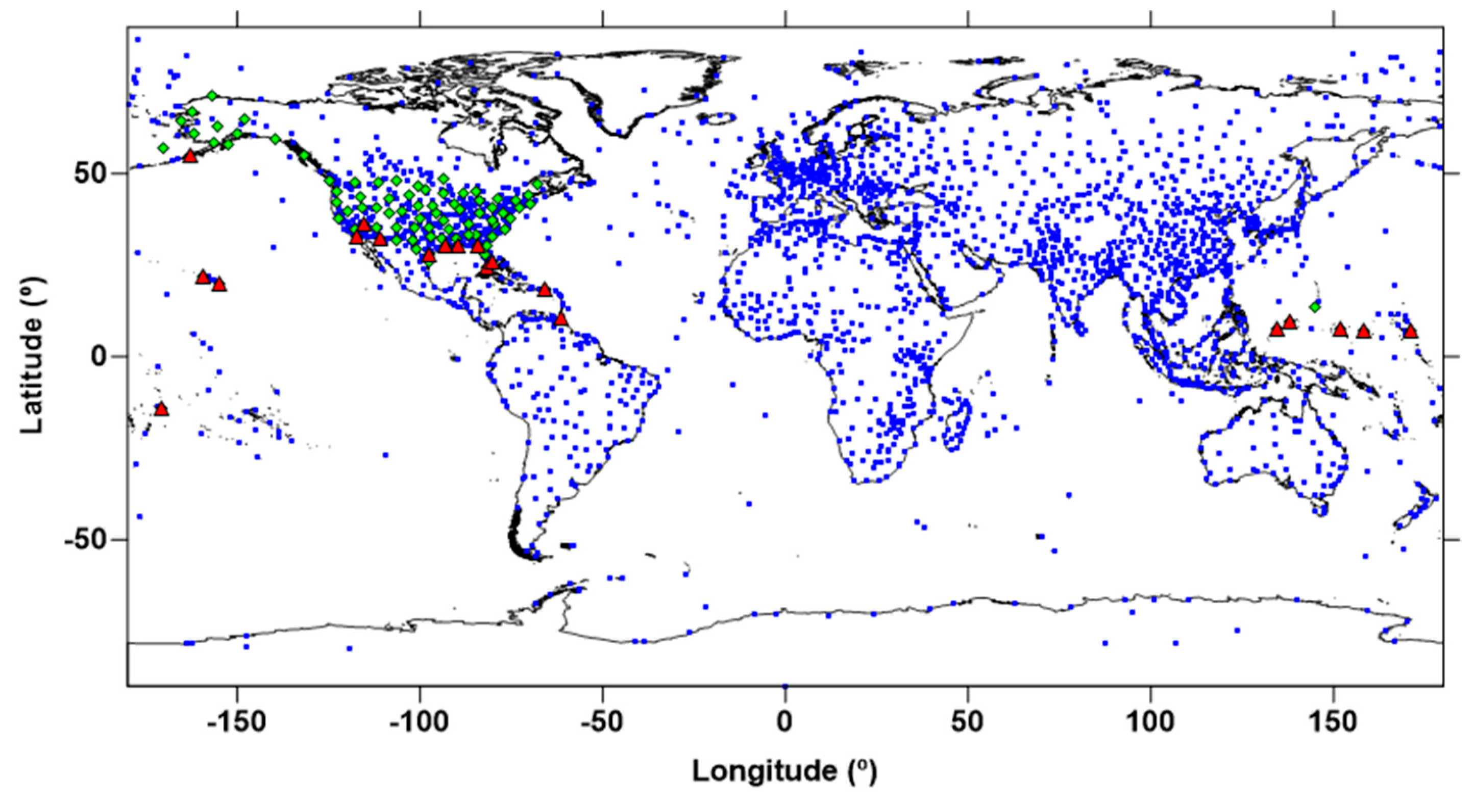
Figure 3 shows the spatial coverage of the radiosondes from IGRA, where blue points represent the 2788 radiosondes since 1905 until 2018. Green diamonds represent the 93 radiosondes with valid measurements of temperature and humidity, as reported in the original sounding, over the year 2014. Within this subset of RS with valid measurements of interest for this study, 20 sites were selected (represented by red triangles) for the validation task. This selection aimed at ensuring a good geographic distribution allowed by the available RS represented by green squares, at low latitudes. Here the WPD is more variable and, thus, the effect of this modelling can be more significant.

2.1.3. GNSS Stations

In the context of the tropospheric corrections for satellite altimetry, despite their poor spatial resolution, GNSS data have been widely used to derive these corrections [12,14]. The increasing number of GNSS stations in coastal zones has been useful for the retrieval of tropospheric corrections in these zones, where the WPD retrieval from MWR measurements become invalid and cannot be used [12]. The GNSS-derived WPD have been adopted for assessment, validation, and monitoring purposes [12,37,42,43,44] and also to develop improved methodologies to provide valid WPD measurements in regions where MWR-derived WPD are invalid [16,17,18].

The WPD is not a direct estimation from GNSS. The quantity derived from this technique is the zenith tropospheric delay (ZTD), which is the total tropospheric delay in the zenith direction due to the dry and wet troposphere. The dry component of the total delay can be computed from surface pressure fields provided by atmospheric models with high accuracy [14]. Using the total delay from GNSS and subtracting the dry delay computed from NWM, both with high accuracy, the WPD can be obtained. This way, at the location of each GNSS station and for each instant, a WPD with an error less than 1 cm is estimated. In terms of vertical reference, these WPD estimations are relative to the corresponding GNSS station height, which is not the level of interest for coastal satellite altimetry application. After the WPD derivation from GNSS, the corresponding estimations must be reduced to the altitude of interest (sea level or water body height), this being a crucial step. Therefore, the modelling of the vertical dependence of the WPD is an important procedure to ensure a better use of GNSS-derived WPD in satellite altimetry.

For more details about the estimation of WPD from GNSS see e.g., [12,14].

2.2. Modelling the Altitude Dependence of the WPD

There is, presently, only one expression available for modelling the WPD vertical dependence, which is the one proposed by Kouba [20]. This expression has many limitations since it considers the same dependence, irrespective of geographic location and WPD variability. Building upon this expression and considering the complex WPD variation, this section presents the developed methodology in view to derive improved expressions, taking into account the different patterns of the WPD vertical variation function of location and time.

2.2.1. The Kouba Formulation

To compare wet delays at different heights and in the absence of a convenient transformation, Kouba [20] developed an exponential decay function to transform wet delays between different altitudes, at the same planimetric point:

$$WP{D}_i=WP{D}_0{e}^{\frac{h_0-h_i}{2000}},$$

(4)

where WPD₀ is the known wet delay at height h₀, and WPD_i is the wet delay to be calculated at height h_i. The Kouba empirical decay coefficient (1/2000) was obtained from the WPD values spanning 1.5 years at a single location (22.13°N, 159.66°W) and at only two levels (ellipsoidal heights 18 and 1168 m). This dataset, considered adequate in the context of the Kouba’s study, is not enough to characterize the complex 4-D WPD variation.

From the analysis of this expression, the following values can be withdrawn: for a WPD of 30 cm at an altitude of 0 m, reducing this value with the Kouba expression to an altitude of 1000 m, the corresponding WPD is 18.2 cm. For empirical decay coefficients of, for example, 1/1500 or 1/2500, the corresponding WPD is 15.4 or 20.1 cm, respectively. Therefore, the effect of using different decay coefficients can lead to WPD differences of several centimeters.

2.2.2. Modelling Using ERA5 Data on Pressure Levels

After analyzing the sensitivity of the Kouba expression concerning its decay coefficient and given the high 4-D WPD variation, new decay coefficients will be modelled in this section. Hereafter, for simplification, instead of a decay coefficient (which for Kouba is 1/2000), an inverse decay coefficient (α) is introduced.

In a 5° × 5° grid, WPD vertical profiles were computed from atmospheric variables on PL from ERA5, over 4 years, as described in Section 2.1.1. A temporal sampling of 3h was used, considered to be adequate for the WPD computation [30]. At each location and for each WPD vertical profile, an α coefficient is determined using least squares, setting the initial coefficient to the Kouba value (2000). Since the main application of this modelling is satellite altimetry over coastal and inland waters, only the altitudes below 4000 m are of interest. For this reason, only pressure levels with altitudes below 4000 m were considered. On the other hand, only the pressure levels above surface were selected, as those below the surface are generated by extrapolation. For regions where the surface height is larger than 4000 m (e.g., Himalayas region), the corresponding vertical profiles will be empty and the initial coefficient (2000) was considered for these cases.

Thus, for each point in a 5° × 5°grid, an α coefficient was determined every 3h, from the beginning of 2010 to end of 2013. Analyzing the time series of these coefficients at each point and observing that some regions exhibit an annual signal, as will be addressed in Section 3, three sets of coefficients were developed:

• UP-01: a single coefficient for each location (non-time-dependent), computed as the mean at each point;
• UP-04: four seasonally averaged coefficients for each location;
• UP-12: 12 monthly averaged coefficients for each location.

The computation of the UP-04 and UP-12 coefficients was performed by binning the coefficients into classes of time intervals (4 months and 1 month, respectively), spanning the four analyzed years. Results in Section 3 will show that using data for only one year, the obtained coefficients are very similar, without significant differences from those obtained using the 4-year dataset. For this reason, the time span used for this modelling (4 years) is considered appropriate, since additional years do not generate different coefficients.

2.2.3. Assessment and Validation

After introducing Kouba’s expression and developing the UP modelling, the proximity of the WPD vertical profiles computed from ERA5 data on PL and those derived from WPD at only one vertical level, followed by different altitude reductions (both Kouba and UP) was analyzed. For this purpose, ERA5 data on PL for a different period, i.e., for a time span not used in the UP modelling was selected.

Two WPD vertical profiles were considered, at each 5° × 5° grid point, every 3h: the first one computed from ERA5 data on pressure levels from Equation (3) and the second one estimated at ERA5 orography level from Equations (1) and (2), further reduced to the upper pressure levels using the different modelling approaches (Kouba, UP-01, UP-04, and UP-12). The differences between the computed WPD vertical profiles from ERA5 data (temperature and humidity fields) and those reduced from the values at surface level will provide a global quantification of the ability of the different modelling approaches to describe the WPD vertical distribution, knowing only one WPD value at surface level.

The validation of the various expressions was performed by means of independent data from radiosondes and GNSS stations.

For the validation from radiosondes, a similar procedure used in the assessment with ERA5 was adopted. Two WPD vertical profiles were selected. The first one was computed from temperature and humidity data from radiosondes on their vertical levels and the other one from the WPD at the lowest RS level and then reduced to the upper levels using the different coefficients. This validation was performed by means of independent in-situ atmospheric measurements up to an altitude of 4 km, however it was spatially limited to the network coverage of the RS with valid temperature and humidity measurements.

For the validation using GNSS data, two single level WPD values were selected: one derived from GNSS at the corresponding station level, and the other one computed at ERA5 orography level from Equations (1) and (2) further reduced to the corresponding station height, using the different altitude reductions. This validation was performed at only one level, while the validation with radiosondes was carried out along various vertical profiles in a range of altitudes up to 4 km, so the significance of the validation from RS data is larger than that from GNSS. Moreover, the validation with GNSS data is only useful for GNSS stations with altitudes significantly different from the altitude of the ERA5 orography at the location of the corresponding GNSS station. The validation with GNSS is also limited to the corresponding network spatial coverage. The assessment with ERA5 is the only method that allows a global inspection of the different vertical modelling.

3. Results and Discussion

This section provides a description of the experimental results at each step of this study, as well as the corresponding interpretation and the corresponding discussion.

3.1. Comparison between WPD Computed Using Different ERA5 Data

As described above, ECMWF provides 3-D variables both at model and pressure levels and the first ones lead to a significantly larger computational effort. Before adopting the second ones in this study, an assessment was carried out to inspect the impact of this choice, both in terms of accuracy and computational time. For this purpose, the following WPD were compared at the level of the ERA5 orography: the WPD computed using Equation (3) from temperature and humidity variables provided at pressure and model levels (37 and 137 vertical levels, respectively). For completeness, the WPD retrieved from single level variables using Equations (1) and (2) was also considered. Thus, for a time span of one complete year (2010), three WPD were considered for each point, at the level of ERA5 orography.

To consider the three values at the same vertical reference (ERA5 orography level), when the orography height is between two consecutive pressure levels, the corresponding WPD value from PL data was interpolated to the orography level using the WPD at the corresponding consecutive pressure levels. When the orography height was below the lowest pressure level, the WPD value from data on PL was extrapolated to the orography height. The same procedures were not required for the ML, since the corresponding vertical levels were always above the orographic surface. Thus, the three WPD values computed at each point using different ERA5 data (SL, ML, and PL) under comparison were relative to the same altitude, avoiding the introduction of biases.

Statistical parameters (mean and standard deviation in centimeters) of the differences between these three WPD values were calculated. These statistics reveal very small differences, with standard deviation values not larger than 2 mm and an absolute mean up to 1 mm. Concerning the differences between the two computations using 3-D variables (on model and pressure levels) the mean is null, and the standard deviation is 1 mm, showing an insignificant effect. As suggested by Figure 1, these results indicate that there is no significant impact when the WPD is computed using data on ERA5 pressure levels, instead of denser data on model levels. For this reason and in the interest of computational time, the estimation from data on PL was adopted in this study.

Regarding the differences between the WPD retrieval from single level variables (SL) and those using 3-D variables, there is a small bias (absolute mean of 1 mm). For the case of data on PL, this should be due to the interpolation and extrapolation errors, while for the data on ML, this is due to the altitude of the lowest model level. Computing the global differences between the ERA5 orography height and the altitude of the lowest model level (the first level, closest to the surface), the absolute mean is 9.7 m. This indicates that the lowest model level is systematically 9.7 m above the ERA5 orography height, leading to a very small bias (1 mm).

Considering a compromise between accuracy and computational time, the ERA5 data on pressure levels were selected for this modelling.

3.2. Modelling

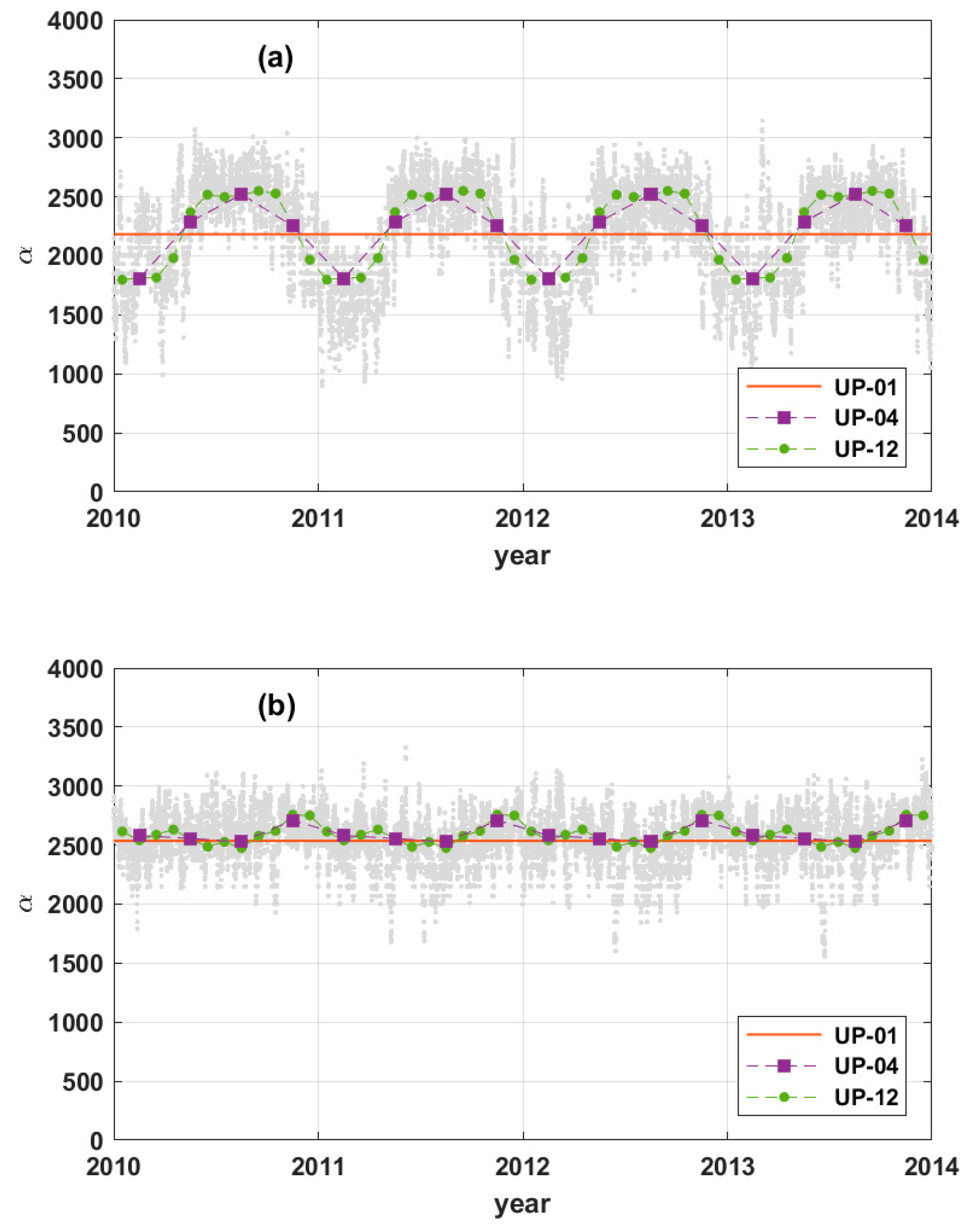
Using the pressure levels above the surface and up to an altitude of 4 km, WPD vertical profiles have been estimated globally, every 3h, for a time span of 4 years. Building upon these vertical profiles, the α coefficient (derived from the empirical decay coefficient in the expression proposed by Kouba [20]) was computed every 3h at each grid point using least squares. Figure 4 represents the time evolution of these α coefficients at three different locations: (a) one point in the northern hemisphere with coordinates 10°N, 90°W; (b) one point in the equator with coordinates 00°, 100°E; (c) one point in the southern hemisphere with coordinates 25°S, 65°E. Three geographic locations, the same as in Figure 2, were chosen to be representative of the global distribution and variability of the α coefficients (which describe the WPD vertical variation). The location in the equator (b) shows a low variability, while the other two locations show high variability.

Analyzing Figure 4, the most striking feature is the clear annual signal observed in the coefficients, more pronounced at locations not over the equator, as illustrated in Figure 4a,c. The signals shown in these panels are not in phase, since they are relative to locations at different hemispheres. The first one is maximum when the second one is minimum. Another striking feature is the high variation of the α coefficients, even for small periods, evidencing the high vertical variation of the WPD. This variability represents an additional difficulty in this modelling.

The three UP modelling approaches (UP-01, UP-04 and UP-12), as described in Section 2, are represented in Figure 4 by orange lines, purple squares, and green circles, respectively. Figure 4a,c shows that the use of a single non-time-dependent coefficient (UP-01) is not enough to account for the variability that the coefficients determined every 3h show.

Assuming an additional temporal dependence (UP-04 and UP-12), the corresponding modelled coefficients can still be very different from those determined every 3h, evidencing again the difficulty of this modelling.

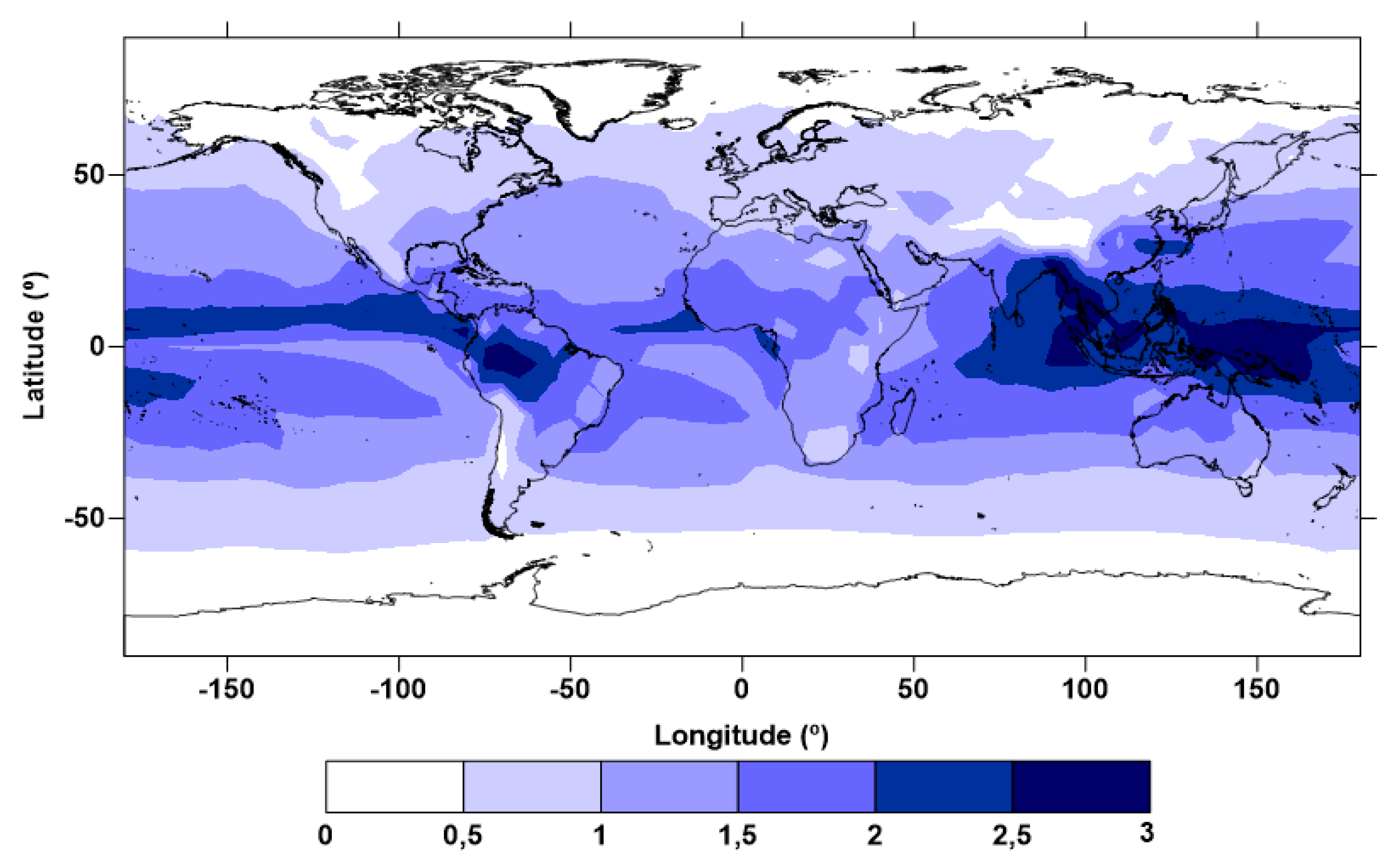
Considering only the spatial dependence of this modelling, Figure 5 shows the spatial representation of the α coefficients derived as the mean for each point, non-time-dependent (UP-01). The color scale of the α coefficient is saturated in the range [1500–2500] in order to have a scale centered in 2000 (white), however the minimum and maximum coefficients are 1165 and 2705, respectively. The most striking feature of this spatial representation is that there are many regions where the α coefficient is very different from that proposed by Kouba. To understand the impact of having different coefficients, taking the example given in Section 2, for a WPD of 30 cm at the zero level, the reduced values at an altitude of 1000 m are 12.7 and 20.7 cm using an α coefficient of 1165 and 2705, respectively. The two WPD at the example level of interest corresponding to the minimum and maximum α coefficients found in the results of this modelling have a difference of 8 cm, a very significant value regarding the accuracy of the WPD derived from the different sources. These values are important indicators of the need of having a vertical modelling of the WPD, dependent on geographic location.

In Figure 5, regions represented in white are those where the α coefficient derived from ERA5 3-D PL data is close to that suggested by Kouba. These regions are mainly over the poles, where the WPD at surface level is small and, for this reason, there is a narrow range of WPD variation, from a small value at surface height (a few cm) up to zero at a certain altitude. The same happens over high regions and for altitudes above 4 km, where the Kouba value is assumed by default in the UP modelling. The WPD is more variable in low latitude regions due to the complex wet equatorial climate, with larger temperatures than in the poles, generating a high evaporation rate and large concentrations of water vapor in the troposphere.

The spatial representation of the α coefficient in Figure 5 gives some information about the atmospheric water vapor concentration. Since this coefficient describes the exponential decrease of the WPD with altitude, according to Equation (4), a small α coefficient makes the WPD vanish more rapidly with altitude, while a large coefficient represents a slower decrease. This means that, when compared with the total atmospheric column at each point, a small α coefficient indicates a larger near-surface water vapor concentration, than a large α coefficient. Thus, regions represented in blue in Figure 5 have larger near-surface water vapor concentrations than regions represented in red.

In summary, UP modelling consists of three sets of α coefficients in a 5° × 5° grid: UP-01, a single coefficient for each point (2701 coefficients represented in Figure 5); UP-04, four seasonally averaged coefficients for each point (10,804 in total); UP-12, 12 monthly averaged coefficients for each point (32,412 in total).

A larger number of coefficients (both in space and time) would certainly lead to a better modelling of the vertical distribution of WPD, however, it is important to find a compromise between accuracy and computational effort. An increasing number of coefficients means an increasing time of computation in the handling of the WPD provided from different sources. The significance of using the different modelling approaches here presented will be addressed below, in view to assess and validate the impact of using the various improved procedures.

3.3. Assessment with ERA5 Data

The assessment carried out using ERA5 data on PL allows a global inspection of the impact of adopting different sets of coefficients in the WPD estimation, when compared with the corresponding WPD retrieved from the original ERA5 PL fields. Five global sets of WPD vertical profiles were considered: one computed at pressure levels adopting the corresponding variables from ERA5 and the other four computed at only one level (ERA5 orography level) further reduced to the various PL using the Kouba and each of the three UP models.

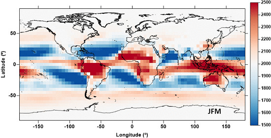
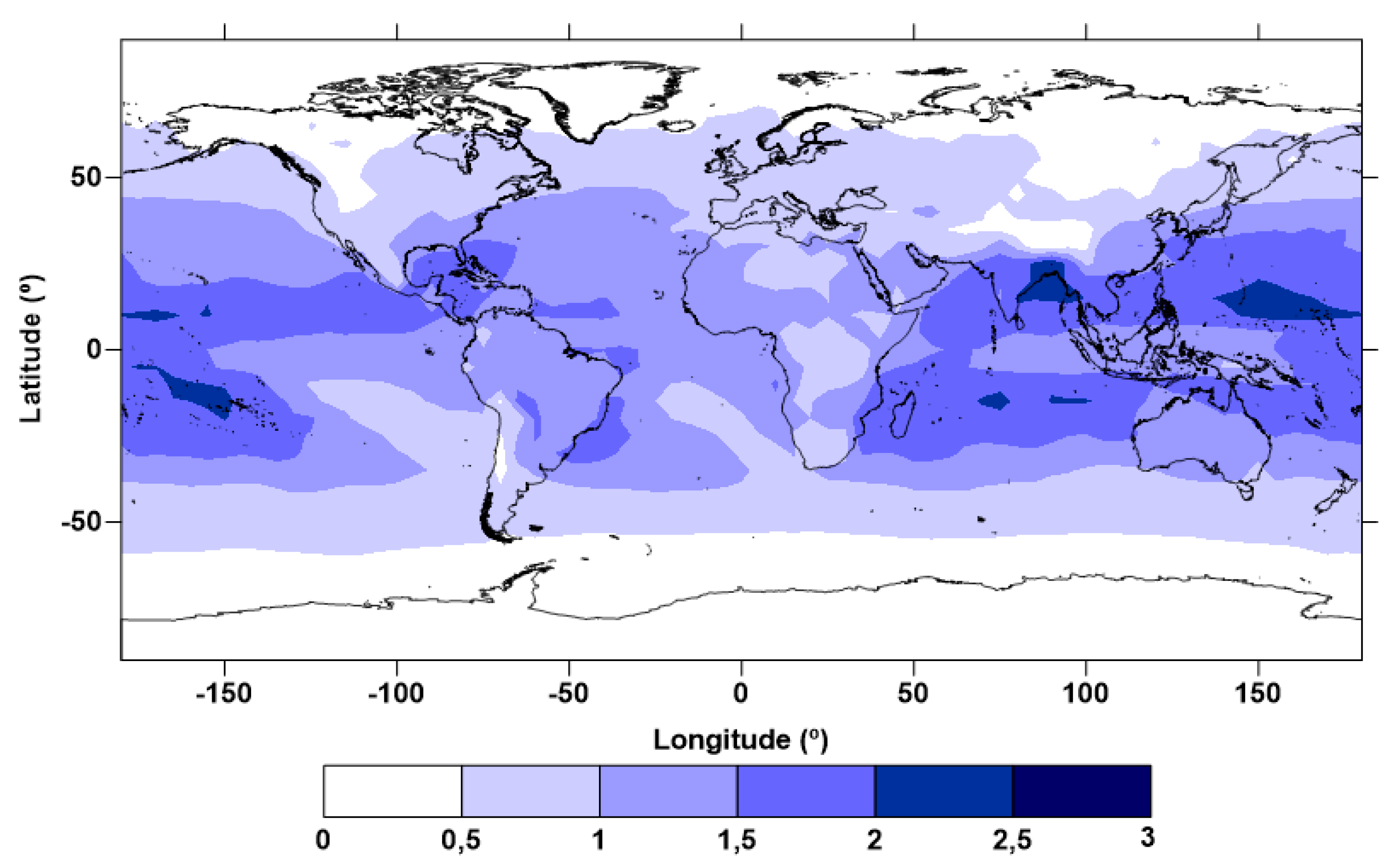
Figure 6 represents the RMS, in centimeters, of the differences between these two WPD vertical profiles (up to 4 km), considering ERA5 data over the year 2014, selecting for the altitude reduction only the α coefficient proposed by Kouba (2000). The largest differences, where the performance of the Kouba coefficient is worst, are observed for low latitudes, represented by dark blue. The maximum RMS value of 3.2 cm is observed at 5°S, 150°E (Papua New Guinea region). The Indonesia region, together with the central Pacific, are the regions where the Kouba coefficient has the largest errors, when compared with WPD retrieved from ERA5 data on PL. The coastal zones, as the Indonesia region [10] and the central America, are the critical regions where better vertical modelling is required.

Figure 7 represents the same as Figure 6, but using UP-01 coefficients for the altitude reduction, instead of Kouba. The clearest observation is the RMS decrease when a spatially dependent coefficient (UP-01) is used, in place of a single coefficient (Kouba). This RMS decrease is clearer over the Indonesia region. To the maximum RMS difference of 3.2 cm observed at 5°S, 150°E in Figure 6 (with the Kouba approach) corresponds a value of 1.2 cm in the UP-01 modelling, leading to an RMS decrease of 2 cm at this location. Using UP-01, the maximum RMS WPD difference is 2.5 cm at the location with coordinates 25°N, 90°E, where the corresponding Kouba value is 2.7 cm.

The most significant impact of this modelling observed in the Indonesian region, considering only a dependence on geographic location and neglecting the dependence on time (UP-01), is due to the low temporal variability of the WPD over this region. Despite its large absolute values, over this region WPD has a small temporal variability, when compared with the surrounding regions [6] (see the vertical profile of Figure 2b, representative of the WPD variability in this region).

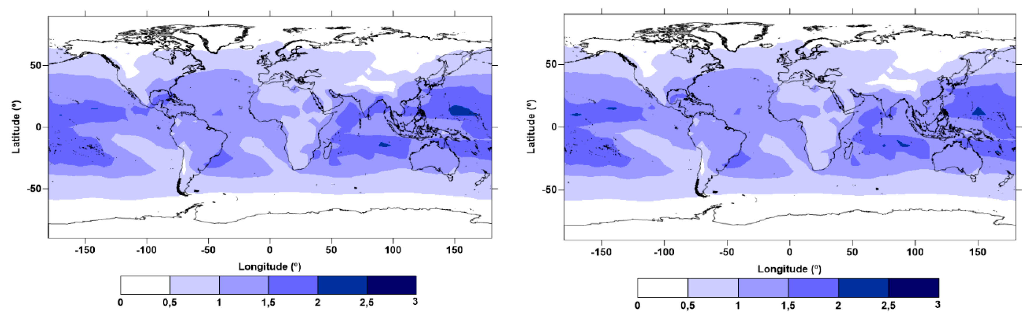
Figure 8 illustrates the same assessment using the UP modelling which considers a temporal dependence of the α coefficients (UP-04 and UP-12), in the left and right panels, respectively. Here, the decrease in the analyzed statistical parameter is not so clear, however the maximum values are 2.2 and 2.1 cm, using UP-04 and UP-12, respectively. Moreover, in the region where the additional temporal modelling has the most significant impact (25°N,90°E, Bay of Bengal region), the RMS errors are 2.7, 2.5, 1.7, and 1.4 cm when Kouba, UP-01, UP-04, and UP-12 are used, respectively. When compared with Kouba, the UP seasonally and monthly coefficients lead to an RMS decrease of 1 and 1.3 cm, respectively, at this location. When compared with a single, non-time-dependent coefficient (UP-01), there is an RMS decrease of 0.8 and 1.1 cm when the two time-dependent modelling approaches are adopted, respectively.

It is important to highlight again that the ERA5 data selected for this assessment are not used in the UP modelling, since they refer to different time spans. However, the evaluation presented here is affected by the fact that the various analyzed WPD are not completely independent and they are not observations. For a complete analysis, a validation by means of independent WPD values from in situ observations is required. This is presented in the next subsection, selecting measurements from radiosondes and GNSS. However, it is important to highlight that the assessment using ERA5 data allows a global analysis, not possible with the data from these independent sources.

3.4. Validation with RS and GNSS

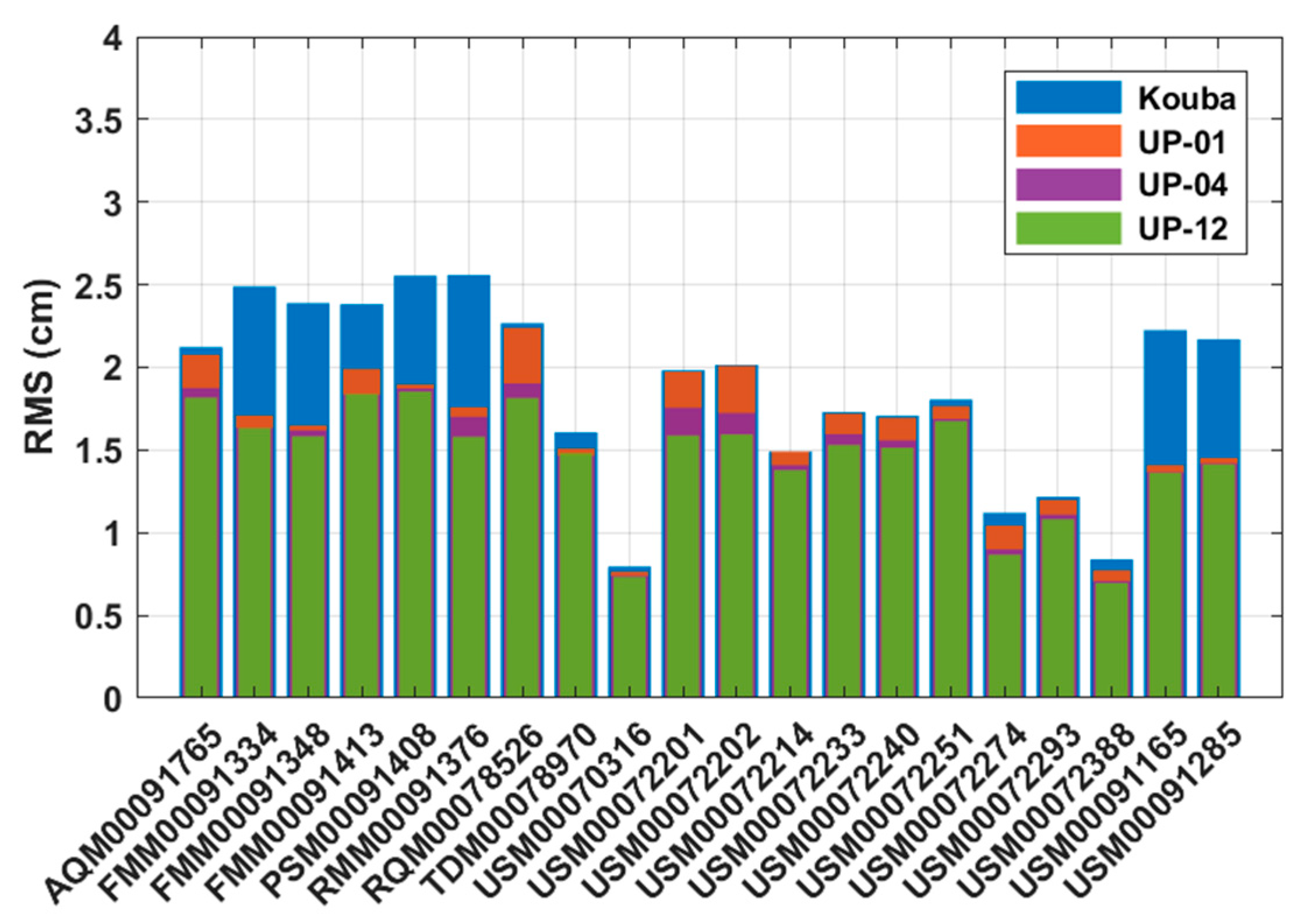
Figure 9 shows the RMS in cm of the differences between WPD computed using data from RS at vertical levels (temperature and humidity) and those using only the WPD at the lowest level of each RS and then reduced to the upper levels through the different modelling approaches: Kouba (blue), UP-01 (orange), UP-04 (purple), and UP-12 (green). These differences are exclusively due to the altitude reduction, since the initial WPD is the same at the lowest level of the RS vertical profile.

The horizontal axis of Figure 9 represents a set of 20 radiosondes selected among the available sites with valid temperature and humidity data. Observing Figure 9, the most significant decrease in the RMS error occurs from Kouba (blue bars) to UP-01 (orange bars), corresponding to the use of spatially dependent coefficients instead of a single coefficient. This effect is significant in radiosondes FMM, PSM, and RMM in the region of Indonesia and in the last two USM in Hawaii, as illustrated in Figure 3. This is in agreement with the results shown in Figure 6 and Figure 7, where the most significant impact of spatially dependent coefficients (UP-01), in comparison with Kouba, is mainly over the Indonesia region and central Pacific.

Moreover, in some regions the additional modelling of the temporal dependence (UP-04 and UP-12) also has a significant impact, when compared with UP-01, as observed mainly in radiosondes RQM, USM00072201, and USM00072202 in central America. The small differences observed in some radiosondes are due to the small WPD values at surface level (e.g., USM00070316 in the northern hemisphere, with a latitude larger than 50°).

These independent in situ data show that the RMS error decrease can be larger than 1 cm in some regions, when using the UP coefficients instead of Kouba’s single coefficient.

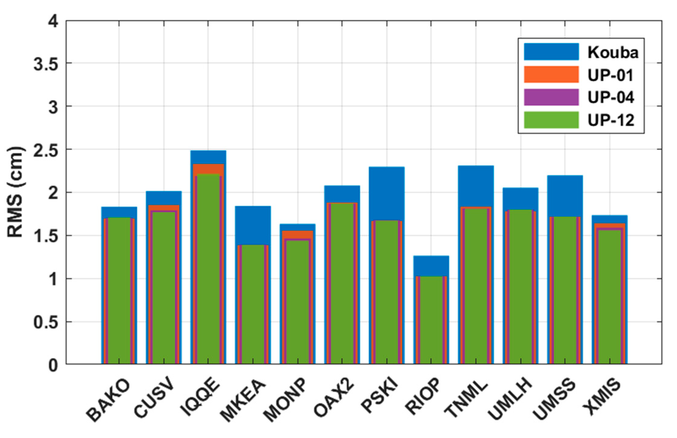
A similar validation was performed using GNSS stations, however this is limited in terms of vertical levels, since it was carried out at only one level, the altitude of each station. Moreover, the differences achieved in this comparison are due to the altitude reduction but also due to the differences between GNSS and ERA5. On the other hand, this validation is significant only for GNSS stations with altitudes very different from the ERA5 orography, at the corresponding GNSS location. Figure 10 shows the RMS in cm of the differences between WPD derived from GNSS and that computed from ERA5 data at the corresponding orography level and then reduced to the altitude of the station, adopting the different modelling approaches represented by the same colors. The results given in Figure 10 are very similar to those given in the validation with radiosondes. This comparison with GNSS does not give additional significant information. It is important to note that WPD derived from ERA5 have an accuracy worse than those derived from GNSS. The WPD value (from ERA5) is the same in the different altitude reductions, so even with an improved methodology the initial value has a low accuracy. The results shown in Figure 10 are affected by this issue, which does not happen in the validation using RS.

The global assessment with ERA5 data and mainly the validation with in situ radiosondes at vertical levels show the significant impact of the modelling presented in this study, when compared with the only modelling available so far [20]. The new UP models must be adopted to reduce WPD values at undesirable altitudes, e.g., those provided at the level of NWM orography in some altimetry products [5,11]. One of the applications of these models will be the integration in the GNSS-derived Path Delays Plus (GPD+) algorithm [16,17,18], which provides valid WPD measurements whenever the corresponding path delay derived from MWR is invalid or inexistent. This method combines different data sources (e.g., GNSS) in the vicinity of each along-track point with invalid or inexistent MWR-derived WPD. These new models will be implemented in this algorithm to better combine the different data sources, properly referring the wet correction to the levels of interest for satellite altimetry application (e.g., sea level in coastal oceanic regions [45,46,47]).

The modelling proposed in this study was performed using global 3-D WPD estimations from ERA5. It has long been recognized that the WPD derived from meteorological models has worse accuracy than observations from dedicated instruments [30], however, atmospheric models provide global data to compute 3-D WPD and the quality of the recent models has been increasing significantly.

The option to follow the expression proposed by Kouba for this modelling, deriving improved decay coefficients dependent on geographic location and time (period of the year), was based on the observed exponential variation of the WPD with altitude, as represented in Figure 2. Other types of modelling approaches/functions can be attempted in future work, however, due to the highly WPD vertical variation, as depicted in Figure 4, the development of improved models, namely using piecewise functions, will be difficult. Moreover, models with a larger number of coefficients will result in WPD altitude reduction procedures computationally more intensive.

4. Conclusions

This study presents the modelling of the altitude dependence of the WPD, crucial to better combine the different WPD sources in coastal and continental waters. This way, improved WPD estimations lead to improved water surface height retrievals from satellite altimetry.

This modelling was performed from ERA5, the latest ECMWF reanalysis, shown to be considerably better than ERA Interim in the computation of radar altimeter wet path delays. When compared to ERA Interim, ERA5 leads to a global reduction of the WPD RMS error of 0.2 cm, with values up to 0.4 cm for some latitude bands.

Following the unique expression available for this altitude reduction, the decay coefficient of this exponential expression was modelled, considering a dependence on geographic location and period of the year. This was performed by means of WPD vertical profiles, computed globally, from temperature and humidity 3-D fields provided by ERA5. This modelling consists of an exponential function with variable coefficients. Three models were developed, with different sets of coefficients: UP-01, a single coefficient for each point (non-time-dependent), computed as the mean at each point; UP-04, four seasonally averaged coefficients for each location, and UP-12, 12 monthly averaged coefficients for each point.

Analyzing the time evolution of the coefficients at each location, the first striking feature is the large variation of these coefficients, due to the high WPD vertical variability, which makes this modelling difficult. In some regions, a clear annual signal in the coefficients is observed, suggesting the inclusion of a temporal dependence.

After the modelling, a global assessment using ERA5 data for a different time span was carried out. When compared with an invariable coefficient (Kouba), the most significant RMS error decrease appears when only spatially dependent coefficients (UP-01) are used. This assessment also shows that for the location where the Kouba coefficient has the maximum RMS error of 3.2 cm (around the Indonesia region), this value is reduced to 1.2 cm when UP coefficients are adopted. The most significant impact of this modelling is an RMS decrease of 2 cm. In some regions (e.g., Bay of Bengal), the modelling of the additional temporal dependence (UP-04 and UP-12) has an impact when compared with UP-01. In the region where this temporal modelling has the most significant impact, the RMS error is 2.7, 2.5, 1.7, and 1.4 cm when Kouba, UP-01, UP-04, and UP-12 are considered, respectively. Selecting UP-04 and UP-12 instead of UP-01, the RMS decrease is 0.8 and 1.1 cm, respectively. This assessment also reveals many regions where the additional temporal coefficients have no impact (e.g., European region).

Finally, independent comparisons with radiosondes and GNSS data show that the RMS error decrease can be larger than 1 cm, when UP coefficients are used instead of Kouba. The validation with in-situ measurements obtained from radiosondes is more significant than that with GNSS, since the former are available at various vertical levels and only the altitude reduction is evaluated. On the contrary, the validation with GNSS data was performed at only one vertical level (GNSS station height) and the comparison is affected by the altitude reduction and the expected differences between GNSS and ERA5 derived WPD.

In order to better combine the different WPD data sources (e.g., in the GPD+ algorithm) for satellite altimetry application over coastal and inland waters, the models developed in this study may be adopted, thus contributing to a better retrieval of water surface heights over these regions of interest.

References

- Chaboureau, J.P.; Chédin, A.; Scott, N.A. Remote sensing of the vertical distribution of atmospheric water vapor from the TOVS observations: Method and validation. J. Geophys. Res. Atmos. 1998, 103, 8743–8752. [Google Scholar] [CrossRef] [Green Version]
- Chelton, D.B.; Ries, J.C.; Haines, B.J.; Fu, L.-L.; Callahan, P.S. Satellite Altimetry. In Satellite Altimetry and Earth Sciences: A Handbook of Techniques and Applications; Fu, L.L., Cazenave, A., Eds.; Academic Press: San Diego, CA, USA, 2001; pp. 1–131. ISBN 9780080516585. [Google Scholar]
- Ablain, M.; Cazenave, A.; Larnicol, G.; Balmaseda, M.; Cipollini, P.; Faugère, Y.; Fernandes, M.J.; Henry, O.; Johannessen, J.A.; Knudsen, P.; et al. Improved sea level record over the satellite altimetry era (1993–2010) from the Climate Change Initiative project. Ocean Sci. 2015, 11, 67–82. [Google Scholar] [CrossRef] [Green Version]
- Legeais, J.-F.; Ablain, M.; Zawadzki, L.; Zuo, H.; Johannessen, J.A.; Scharffenberg, M.G.; Fenoglio-Marc, L.; Fernandes, M.J.; Andersen, O.B.; Rudenko, S.; et al. An improved and homogeneous altimeter sea level record from the ESA Climate Change Initiative. Earth Syst. Sci. Data 2018, 10, 281–301. [Google Scholar] [CrossRef] [Green Version]
- Fernandes, M.J.; Lázaro, C.; Nunes, A.L.; Scharroo, R. Atmospheric corrections for altimetry studies over inland water. Remote Sens. 2014, 6, 4952–4997. [Google Scholar] [CrossRef] [Green Version]
- Vieira, E.; Lázaro, C.; Fernandes, M.J. Spatio-temporal variability of the wet component of the troposphere—Application to satellite altimetry. Adv. Space Res. 2019, 63, 1737–1753. [Google Scholar] [CrossRef] [Green Version]
- Brown, S. A novel near-land radiometer wet path-delay retrieval algorithm: Application to the Jason-2/OSTM Advanced Microwave Radiometer. IEEE Trans. Geosci. Remote Sens. 2010, 48, 1986–1992. [Google Scholar] [CrossRef]
- Fernandes, M.J.; Lázaro, C. Independent assessment of Sentinel-3A wet tropospheric correction over the open and coastal ocean. Remote Sens. 2018, 10, 484. [Google Scholar] [CrossRef] [Green Version]
- Cipollini, P.; Benveniste, J.; Birol, F.; Joana Fernandes, M.; Obligis, E.; Passaro, M.; Ted Strub, P.; Valladeau, G.; Vignudelli, S.; Wilkin, J. Satellite altimetry in coastal regions. In Satellite Altimetry over Oceans and Land Surfaces; CRC Press: Boca Raton, FL, USA, 2017; pp. 343–380. [Google Scholar]
- Handoko, E.Y.; Fernandes, M.J.; Lázaro, C. Assessment of altimetric range and geophysical corrections and mean sea surface models-Impacts on sea level variability around the Indonesian seas. Remote Sens. 2017, 9, 102. [Google Scholar] [CrossRef] [Green Version]
- Vieira, T.; Fernandes, M.J.; Lázaro, C. Analysis and retrieval of tropospheric corrections for CryoSat-2 over inland waters. Adv. Space Res. 2018, 62, 1479–1496. [Google Scholar] [CrossRef]
- Vieira, T.; Fernandes, M.J.; Lazaro, C. Independent Assessment of On-Board Microwave Radiometer Measurements in Coastal Zones Using Tropospheric Delays from GNSS. IEEE Trans. Geosci. Remote Sens. 2019, 57, 1804–1816. [Google Scholar] [CrossRef]
- Thao, S.; Eymard, L.; Obligis, E.; Picard, B. Comparison of Regression Algorithms for the Retrieval of the Wet Tropospheric Path. IEEE J. Sel. Top. Appl. Earth Obs. Remote Sens. 2015, 8, 4302–4314. [Google Scholar] [CrossRef]
- Fernandes, M.J.; Pires, N.; Lázaro, C.; Nunes, A.L. Tropospheric delays from GNSS for application in coastal altimetry. Adv. Space Res. 2013, 51, 1352–1368. [Google Scholar] [CrossRef]
- Legeais, J.F.; Ablain, M.; Thao, S. Evaluation of wet troposphere path delays from atmospheric reanalyses and radiometers and their impact on the altimeter sea level. Ocean Sci. 2014, 10, 893–905. [Google Scholar] [CrossRef] [Green Version]
- Fernandes, M.J.; Lázaro, C.; Nunes, A.L.; Pires, N.; Bastos, L.; Mendes, V.B. GNSS-derived path delay: An approach to compute the wet tropospheric correction for coastal altimetry. IEEE Geosci. Remote Sens. Lett. 2010, 7, 596–600. [Google Scholar] [CrossRef]
- Fernandes, M.J.; Lázaro, C.; Ablain, M.; Pires, N. Improved wet path delays for all ESA and reference altimetric missions. Remote Sens. Environ. 2015, 169, 50–74. [Google Scholar] [CrossRef] [Green Version]
- Fernandes, M.J.; Lázaro, C. GPD+wet tropospheric corrections for CryoSat-2 and GFO altimetry missions. Remote Sens. 2016, 8, 851. [Google Scholar] [CrossRef] [Green Version]
- Stum, J.; Sicard, P.; Carrère, L.; Lambin, J. Using objective analysis of scanning radiometer measurements to compute the water vapor path delay for altimetry. IEEE Trans. Geosci. Remote Sens. 2011, 49, 3211–3224. [Google Scholar] [CrossRef]
- Kouba, J. Implementation and testing of the gridded Vienna mapping function 1 (VMF1). J. Geod. 2008, 82, 193–205. [Google Scholar] [CrossRef]
- Böhm, J.; Möller, G.; Schindelegger, M.; Pain, G.; Weber, R. Development of an improved empirical model for slant delays in the troposphere (GPT2w). GPS Solut. 2015, 19, 433–441. [Google Scholar] [CrossRef] [Green Version]
- Yao, Y.B.; Hu, Y.F. An empirical zenith wet delay correction model using piecewise height functions. Ann. Geophys. 2018, 36, 1507–1519. [Google Scholar] [CrossRef] [Green Version]
- Li, W.; Yuan, Y.; Ou, J.; He, Y. IGGtrop-SH and IGGtrop-rH: Two improved empirical tropospheric delay models based on vertical reduction functions. IEEE Trans. Geosci. Remote Sens. 2018, 56, 5276–5288. [Google Scholar] [CrossRef]
- Niell, A.E.; Coster, A.J.; Solheim, F.S.; Mendes, V.B.; Toor, P.C.; Langley, R.B.; Upham, C.A. Comparison of measurements of atmospheric wet delay by radiosonde, water vapor radiometer, GPS, and VLBI. J. Atmos. Ocean. Technol. 2001, 18, 830–850. [Google Scholar] [CrossRef] [Green Version]
- Li, Z.; Muller, J.P.; Cross, P. Comparison of precipitable water vapor derived from radiosonde, GPS, and Moderate-Resolution Imaging Spectroradiometer measurements. J. Geophys. Res. Atmos. 2003, 108. [Google Scholar] [CrossRef]
- Flores, A.; Ruffini, G.; Rius, A. 4D tropospheric tomography using GPS slant wet delays. Ann. Geophys. 2000, 18, 223–234. [Google Scholar] [CrossRef]
- Benevides, P.; Nico, G.; Catalao, J.; Miranda, P.M.A. Analysis of Galileo and GPS Integration for GNSS Tomography. IEEE Trans. Geosci. Remote Sens. 2017, 55, 1936–1943. [Google Scholar] [CrossRef]
- Copernicus Climate Change Service Climate Data Store (CDS). Available online: https://cds.climate.copernicus.eu/cdsapp#!/home (accessed on 20 August 2018).
- Dee, D.P.; Uppala, S.M.; Simmons, A.J.; Berrisford, P.; Poli, P.; Kobayashi, S.; Andrae, U.; Balmaseda, M.A.; Balsamo, G.; Bauer, P.; et al. The ERA-Interim reanalysis: Configuration and performance of the data assimilation system. Q. J. R. Meteorol. Soc. 2011, 137, 553–597. [Google Scholar] [CrossRef]
- Vieira, T.; Fernandes, M.J.; Lazaro, C. Impact of the new ERA5 Reanalysis in the Computation of Radar Altimeter Wet Path Delays. IEEE Trans. Geosci. Remote Sens. 2019, 57, 9849–9857. [Google Scholar] [CrossRef]
- Bevis, M.; Businger, S.; Herring, T.A.; Rocken, C.; Anthes, R.A.; Ware, R.H. GPS meteorology: Remote sensing of atmospheric water vapor using the global positioning system. J. Geophys. Res. 1992, 97, 15787–15801. [Google Scholar] [CrossRef]
- Bevis, M.; Businger, S.; Chiswell, S.; Herring, T.A.; Anthes, R.A.; Rocken, C.; Ware, R.H.; Bevis, M.; Businger, S.; Chiswell, S.; et al. GPS Meteorology: Mapping Zenith Wet Delays onto Precipitable Water. J. Appl. Meteorol. 1994, 33, 379–386. [Google Scholar] [CrossRef]
- Mendes, V.B. Modeling the Neutral-Atmosphere Propagation Delay in Radiometric Space Techniques; University of New Brunswick: Fredericton, NB, Canada, 1999. [Google Scholar]
- Boehm, J.; Heinkelmann, R.; Schuh, H. Short note: A global model of pressure and temperature for geodetic applications. J. Geod. 2007, 81, 679–683. [Google Scholar] [CrossRef]
- Lagler, K.; Schindelegger, M.; Böhm, J.; Krásná, H.; Nilsson, T. GPT2: Empirical slant delay model for radio space geodetic techniques. Geophys. Res. Lett. 2013, 40, 1069–1073. [Google Scholar] [CrossRef] [PubMed] [Green Version]
- Collecte Localisation Satellites (CLS). Surface Topography Mission (STM) SRAL/MWR L2 Algorithms Definition, Accuracy and Specification; CLS: Ramonville St-Agne, France, 2011. [Google Scholar]
- Kalakoski, N.; Kujanpää, J.; Sofieva, V.; Tamminen, J.; Grossi, M.; Valks, P. Validation of GOME-2/Metop total column water vapour with ground-based and in situ measurements. Atmos. Meas. Tech. 2016, 9, 1533–1544. [Google Scholar] [CrossRef] [Green Version]
- Anthes, R.A. Regional models of the atmosphere in middle latitudes. Mon. Weather Rev. 1983, 111, 1306–1335. [Google Scholar] [CrossRef] [Green Version]
- Durre, I. Integrated Global Radiosonde Archive v2; Dataset Descr. Version 1.0; NOAA: Silver Spring, MD, USA, 2016; p. 15. [Google Scholar]
- Durre, I.; Yin, X.; Vose, R.S.; Applequist, S.; Arnfield, J. Enhancing the data coverage in the integrated Global Radiosonde Archive. J. Atmos. Ocean. Technol. 2018, 35, 1753–1770. [Google Scholar] [CrossRef]
- Nievinski, F.G.; Santos, M.C. Ray-tracing options to mitigate the neutral atmosphere delay in GPS. Geomatica 2010, 64, 191–207. [Google Scholar]
- Haines, B.J.; Bar-Sever, Y.E. Monitoring the TOPEX microwave radiometer with GPS: Stability of columnar water vapor measurements. Geophys. Res. Lett. 1998, 25, 3563–3566. [Google Scholar] [CrossRef]
- Desai, S.D.; Haines, B.J. Monitoring measurements from the Jason-1 microwave radiometer and independent validation with GPS. Mar. Geod. 2004, 27, 221–240. [Google Scholar] [CrossRef]
- Sibthorpe, A.; Brown, S.; Desai, S.D.; Haines, B.J. Calibration and validation of the Jason-2/OSTM advanced microwave radiometer using terrestrial GPS stations. Mar. Geod. 2011, 34, 420–430. [Google Scholar] [CrossRef]
- Roblou, L.; Lamouroux, J.; Bouffard, J.; Lyard, F.; Le Hénaff, M.; Lombard, A.; Marsaleix, P.; De Mey, P.; Birol, F. Post-processing altimeter data towards coastal applications and integration into coastal models. In Coastal Altimetry; Springer: Berlin/Heidelberg, Germany, 2011; pp. 217–246. [Google Scholar]
- Liu, Y.; Weisberg, R.H.; Vignudelli, S.; Roblou, L.; Merz, C.R. Comparison of the X-TRACK altimetry estimated currents with moored ADCP and HF radar observations on the West Florida Shelf. Adv. Space Res. 2012, 50, 1085–1098. [Google Scholar] [CrossRef]
- Vignudelli, S.; Birol, F.; Benveniste, J.; Fu, L.-L.; Picot, N.; Raynal, M.; Roinard, H. Satellite Altimetry Measurements of Sea Level in the Coastal Zone. Surv. Geophys. 2019, 40, 1319–1349. [Google Scholar] [CrossRef]
Figure 1.
Atmospheric variables provided by ERA5 on 1 January 2010, at 00:00 UTC on model levels (blue) and on pressure levels (orange): (a) temperature (T) in Kelvin and (b) specific humidity (q) in kg/kg at location 00°, 120°E.
Figure 2.
Wet path delay (WPD) vertical profiles at (a) 10°N, 90°W; (b) 00°, 100°E; (c) 25°S, 65°E. Grey profiles represent those every 3h over the year 2010, solid line represents the annual mean profile, squares with dashed line and circles with dotted line represent the mean profiles for January and July, respectively.
Figure 3.
Spatial representation of the radiosondes (RS) network from Integrated Global Radiosonde Data (IGRA). Blue points represent all RS since 1905, green squares represent the RS with valid measurements of temperature and humidity over the year 2014, and red triangles represent those selected for the validation.
Figure 4.
Time evolution of the α coefficients at locations: (a) 10°N, 90°W; (b) 00°, 100°E; (c) 25°S, 65°E. Grey points represent the α coefficients every 3h, orange line represents the overall mean (UP-01) and purple squares and green points represent the seasonally averaged (UP-04) and monthly averaged coefficients (UP-12), respectively.
Figure 5.
Spatial representation of the α coefficient, computed as the mean for each point (UP-01) in a 5° × 5° grid.
Figure 6.
Root Mean Square (RMS) (cm) of the WPD differences between 3-D (WPD retrieved from the original ERA5 PL fields) and 2-D with Kouba reduction, using profiles every 3h in a 5° × 5° grid over the year 2014.
Figure 7.
RMS (cm) of the WPD differences between 3-D and 2-D with UP-01 reduction, using profiles every 3h in a 5° × 5°grid over the year 2014.
Figure 8.
RMS (cm) of the differences between WPD computed with 3-D approach and that computed at surface level and then reduced with UP-04 (left) and UP-12 (right) coefficients.
Figure 9.
RMS (cm) of the differences between WPD computed with 3-D approach using atmospheric variables from IGRA and those computed at lowest level and then reduced with Kouba (blue bars), UP-01 (orange bars), UP-04 (purple bars), and UP-12 (green bars) coefficients.
Figure 10.
RMS (cm) of the differences at Global Navigation Satellite Systems (GNSS) station height between WPD derived from GNSS and those computed at ERA5 orography level using single level atmospheric variables and then reduced with Kouba (blue bars), UP-01 (orange bars), UP-04 (purple bars), and UP-12 (green bars) coefficients to the height of each GNSS station (identified by its four characters).
© 2019 by the authors. Licensee MDPI, Basel, Switzerland. This article is an open access article distributed under the terms and conditions of the Creative Commons Attribution (CC BY) license (http://creativecommons.org/licenses/by/4.0/).
Share and Cite
MDPI and ACS Style
Vieira, T.; Fernandes, M.J.; Lázaro, C. Modelling the Altitude Dependence of the Wet Path Delay for Coastal Altimetry Using 3-D Fields from ERA5. Remote Sens. 2019, 11, 2973. https://doi.org/10.3390/rs11242973
AMA Style
Vieira T, Fernandes MJ, Lázaro C. Modelling the Altitude Dependence of the Wet Path Delay for Coastal Altimetry Using 3-D Fields from ERA5. Remote Sensing. 2019; 11(24):2973. https://doi.org/10.3390/rs11242973
Chicago/Turabian StyleVieira, Telmo, M. Joana Fernandes, and Clara Lázaro. 2019. "Modelling the Altitude Dependence of the Wet Path Delay for Coastal Altimetry Using 3-D Fields from ERA5" Remote Sensing 11, no. 24: 2973. https://doi.org/10.3390/rs11242973
Note that from the first issue of 2016, this journal uses article numbers instead of page numbers. See further details here.