Assessing Spatiotemporal Variations of Sentinel-1 InSAR Coherence at Different Time Scales over the Atacama Desert (Chile) between 2015 and 2018

 , , ,
, , ,
Abstract
:
1. Introduction
2. Materials and Methods
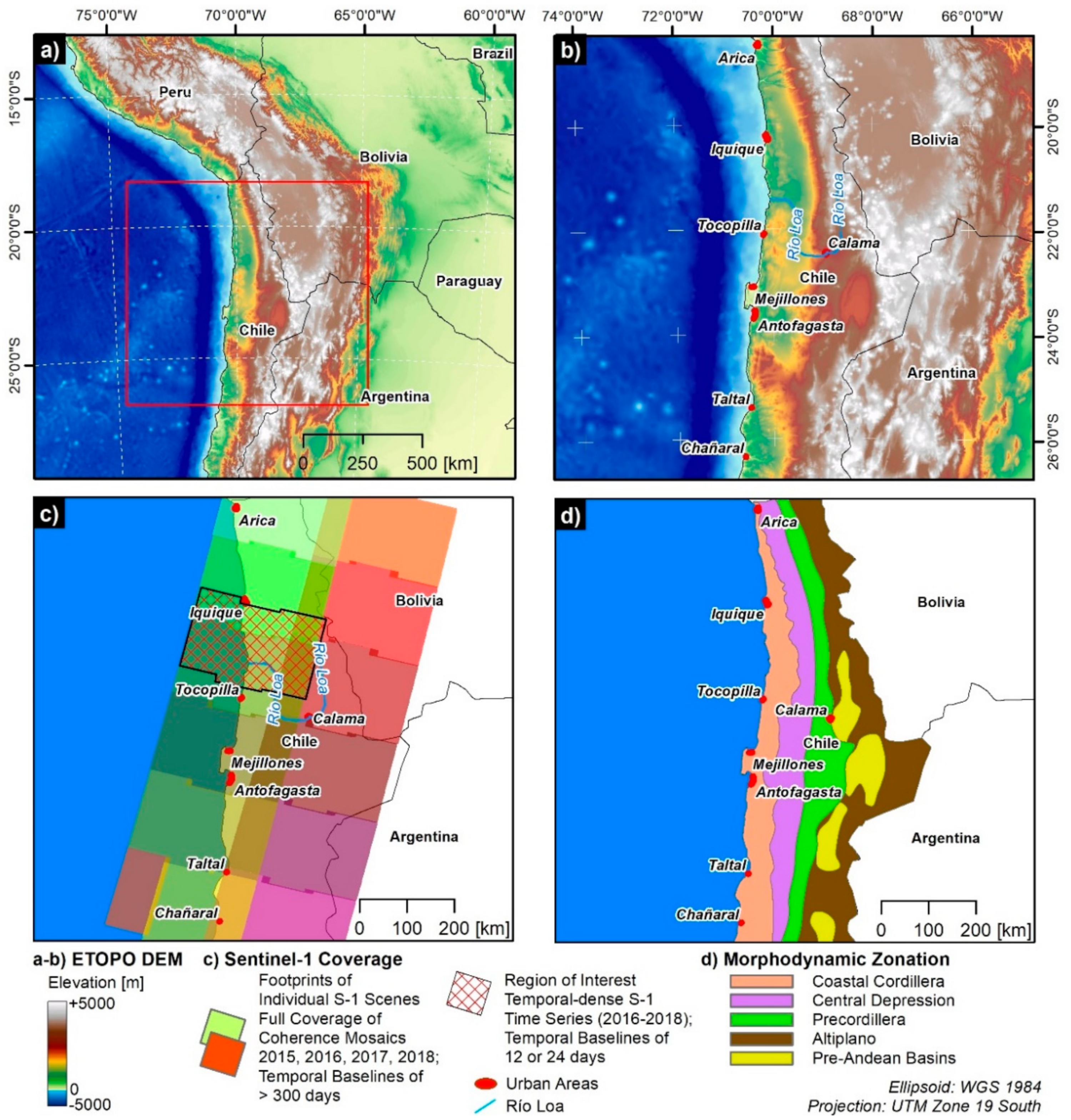
2.1. Study Area
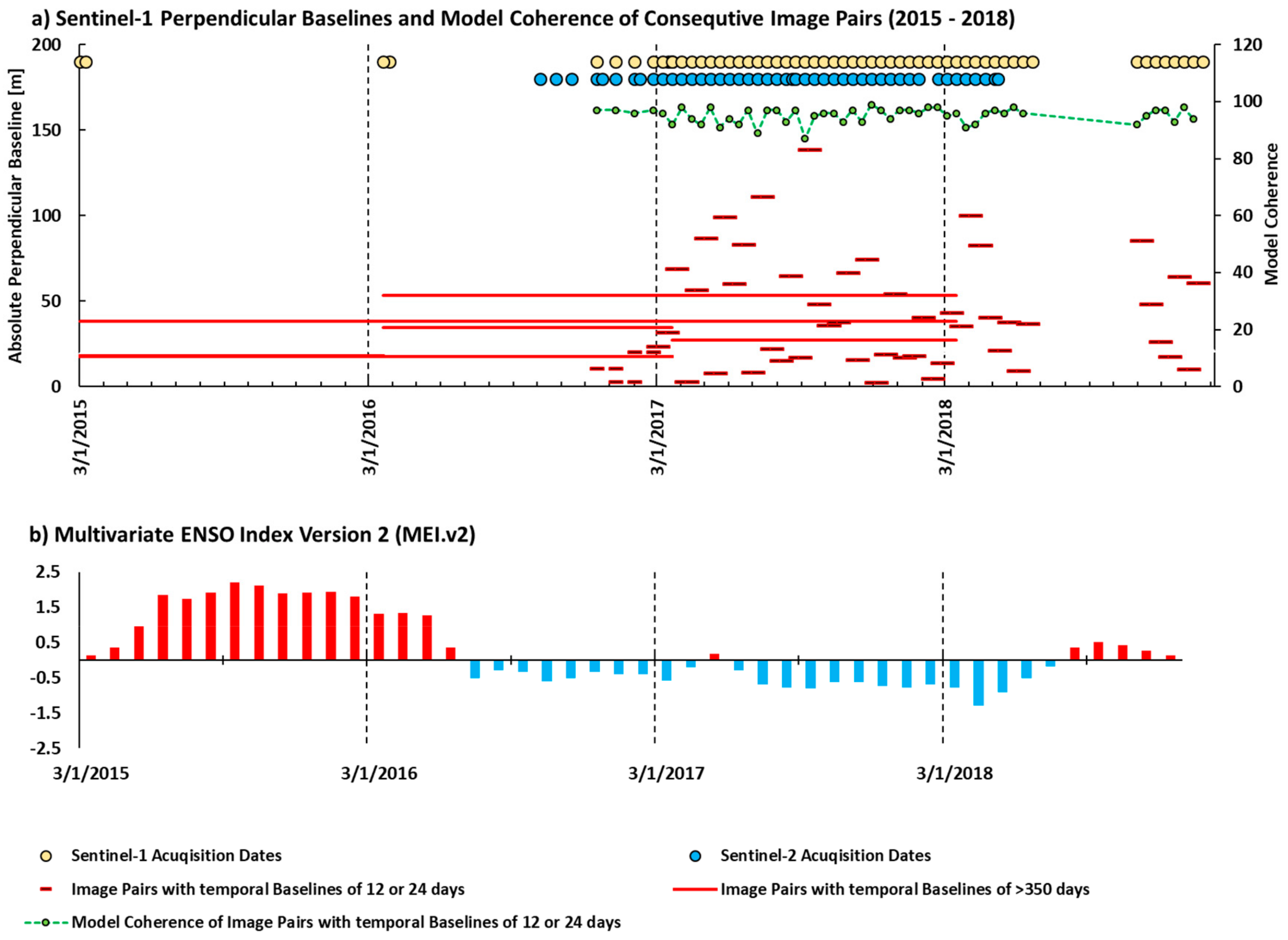
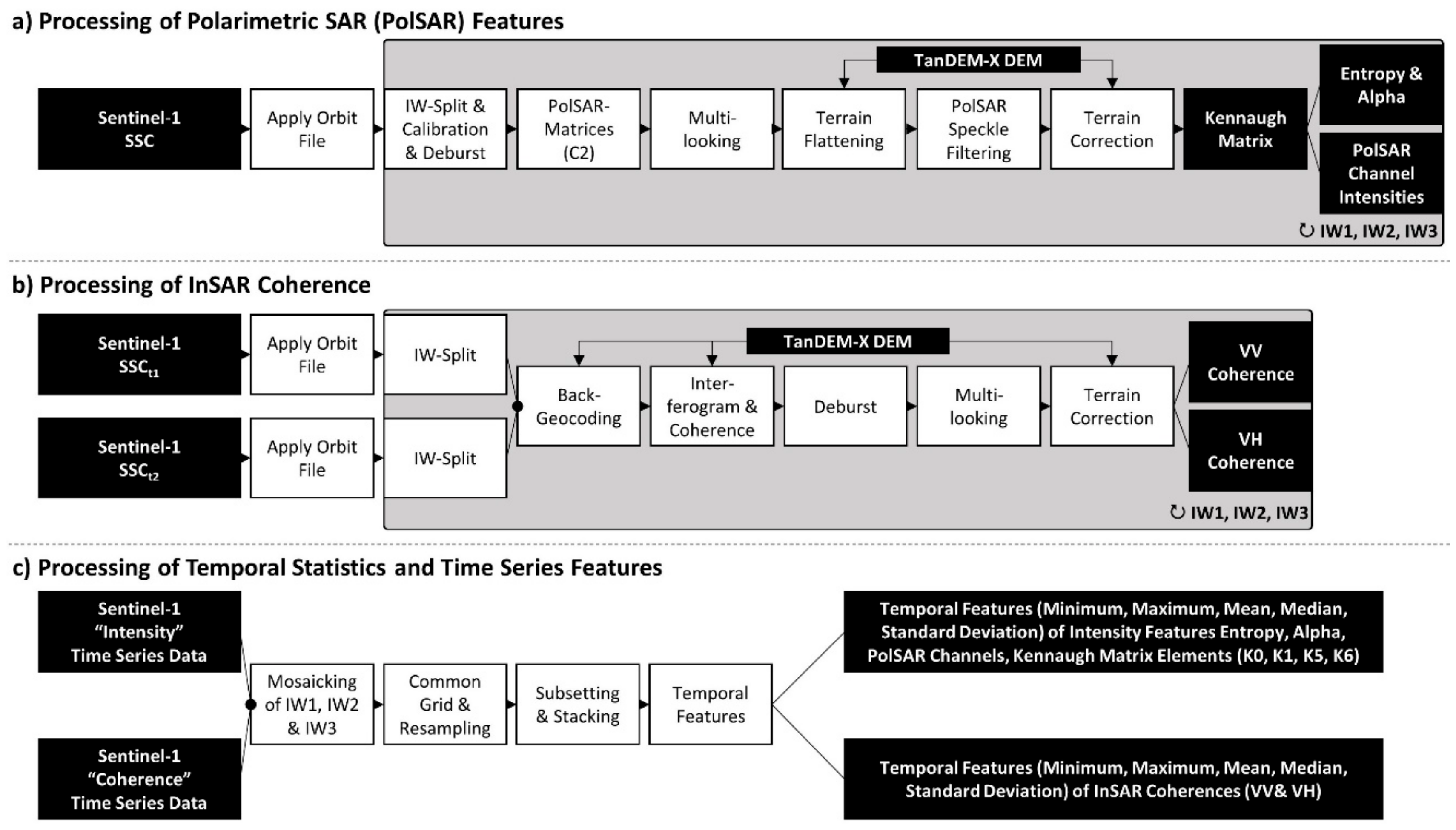
2.2. Sentinel-1
2.3. Reference and Auxiliary Datasets
3. Results
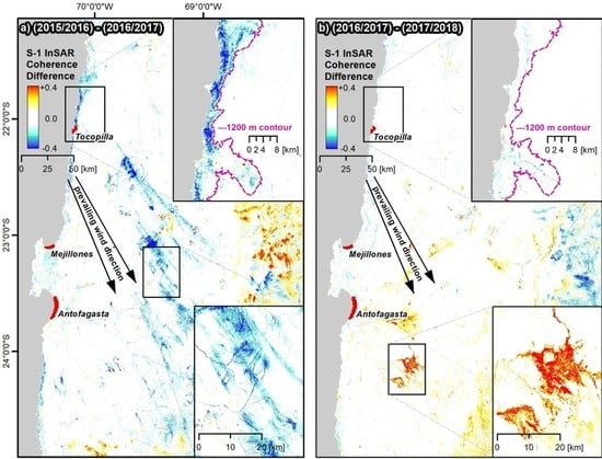
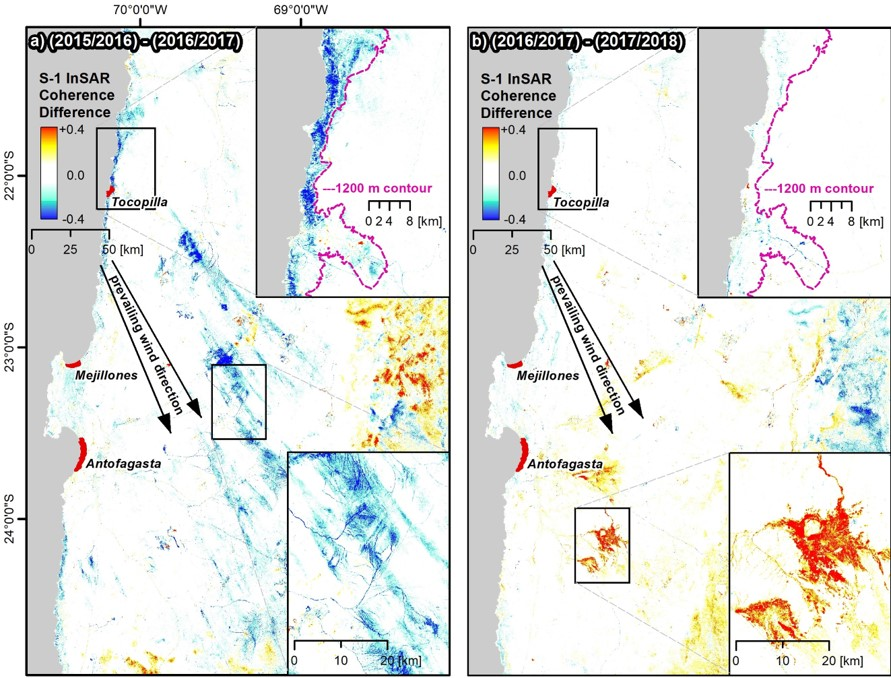
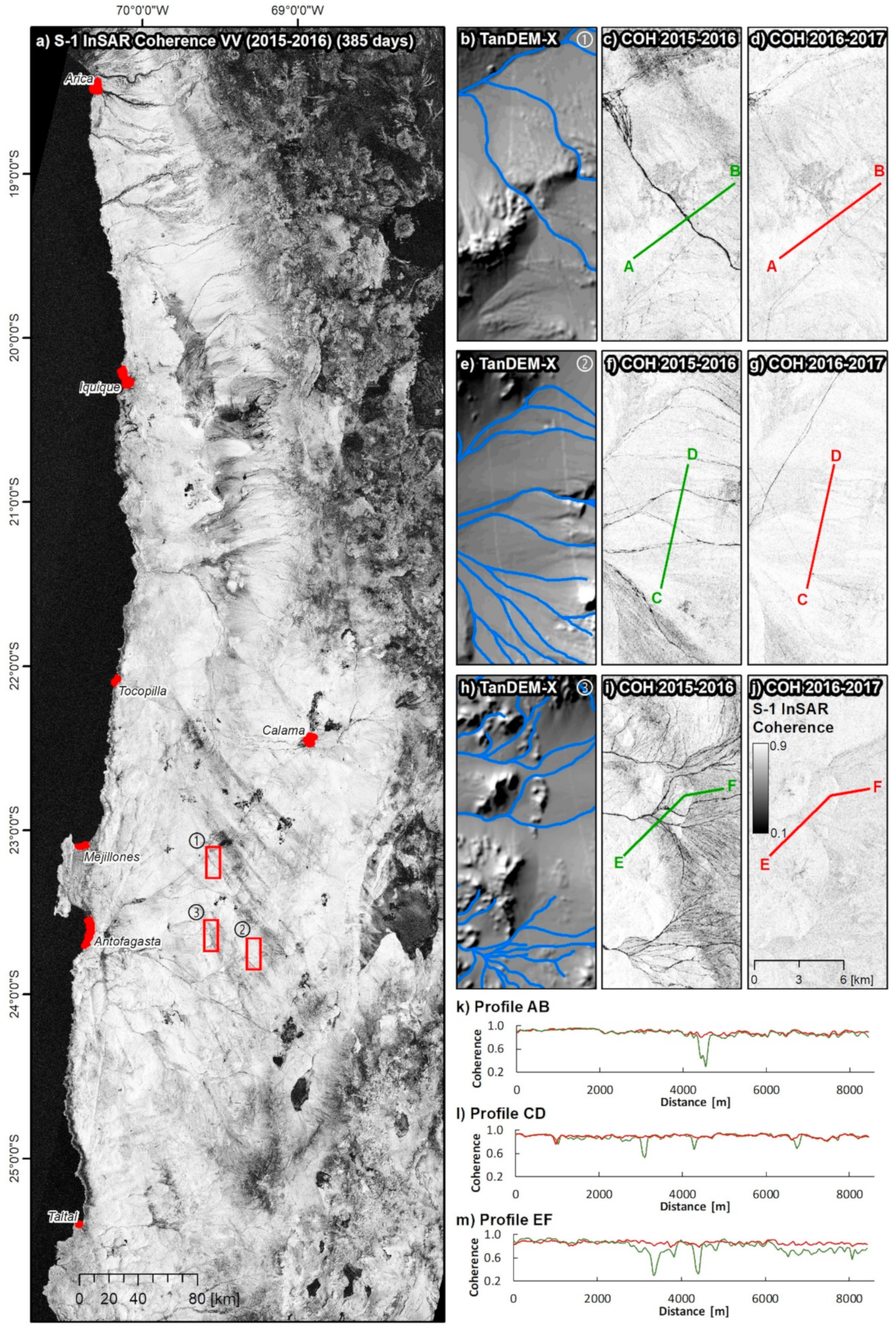
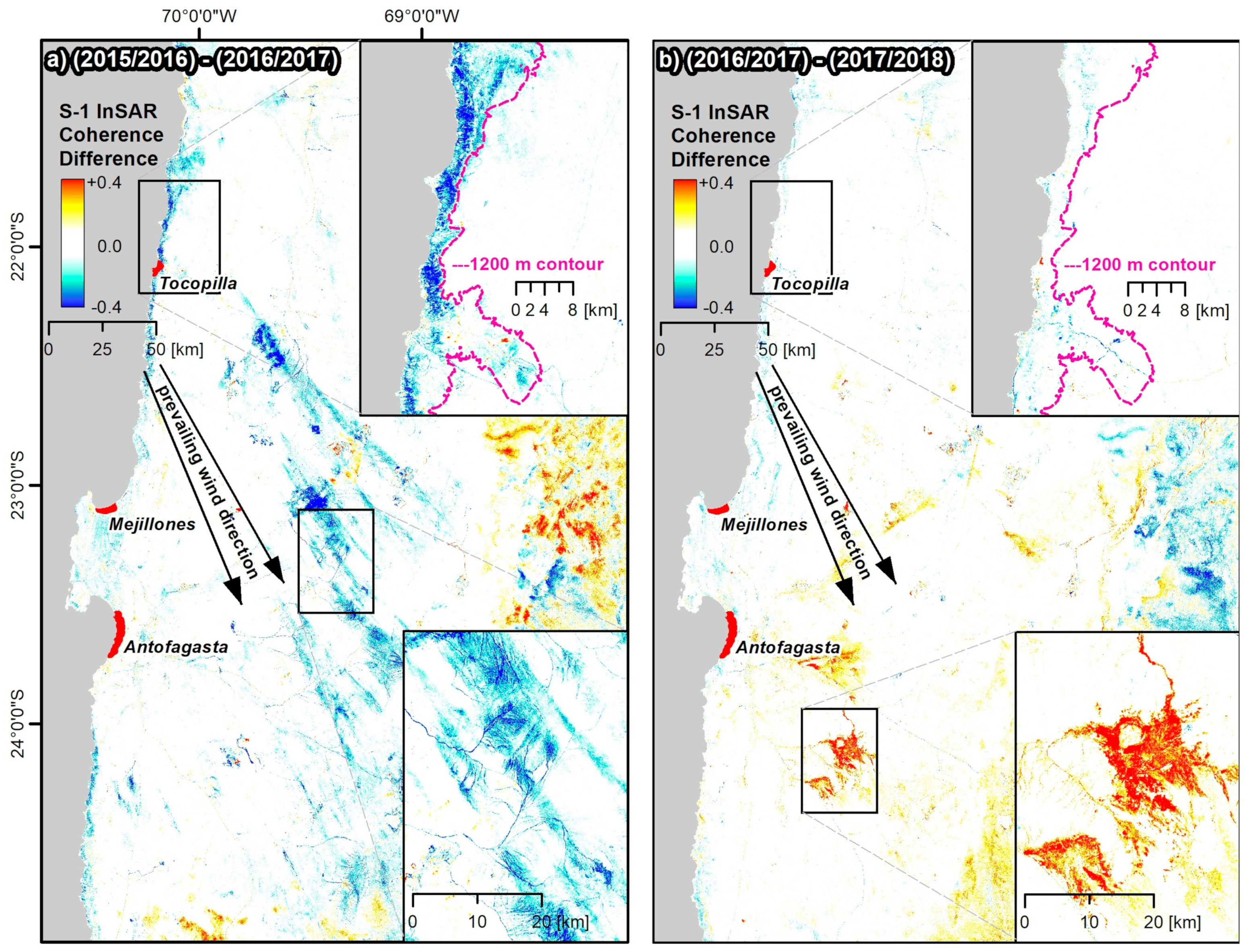
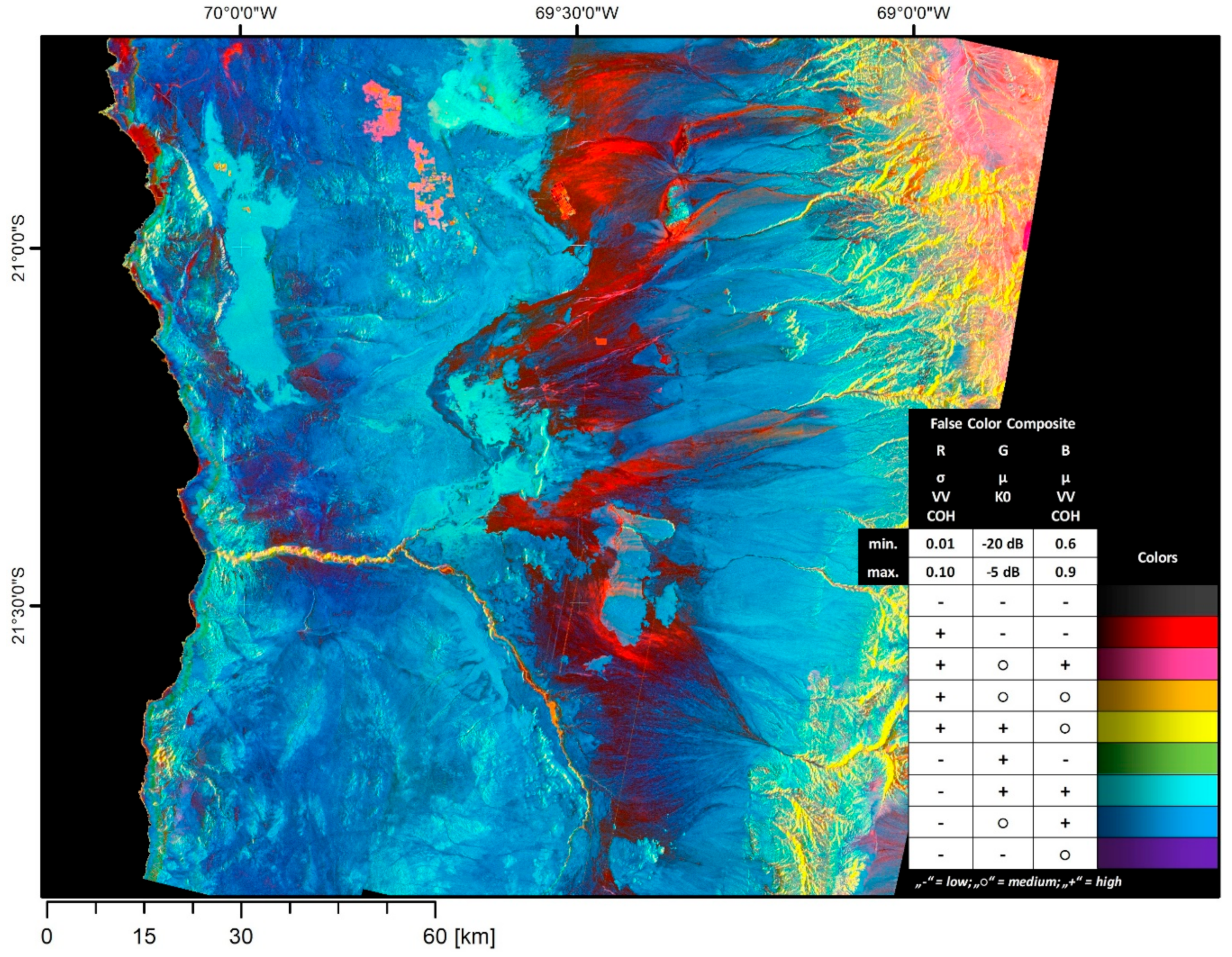
3.1. Sentinel-1—Long Temporal Baselines
3.2. Sentinel-1—Short Temporal Baselines
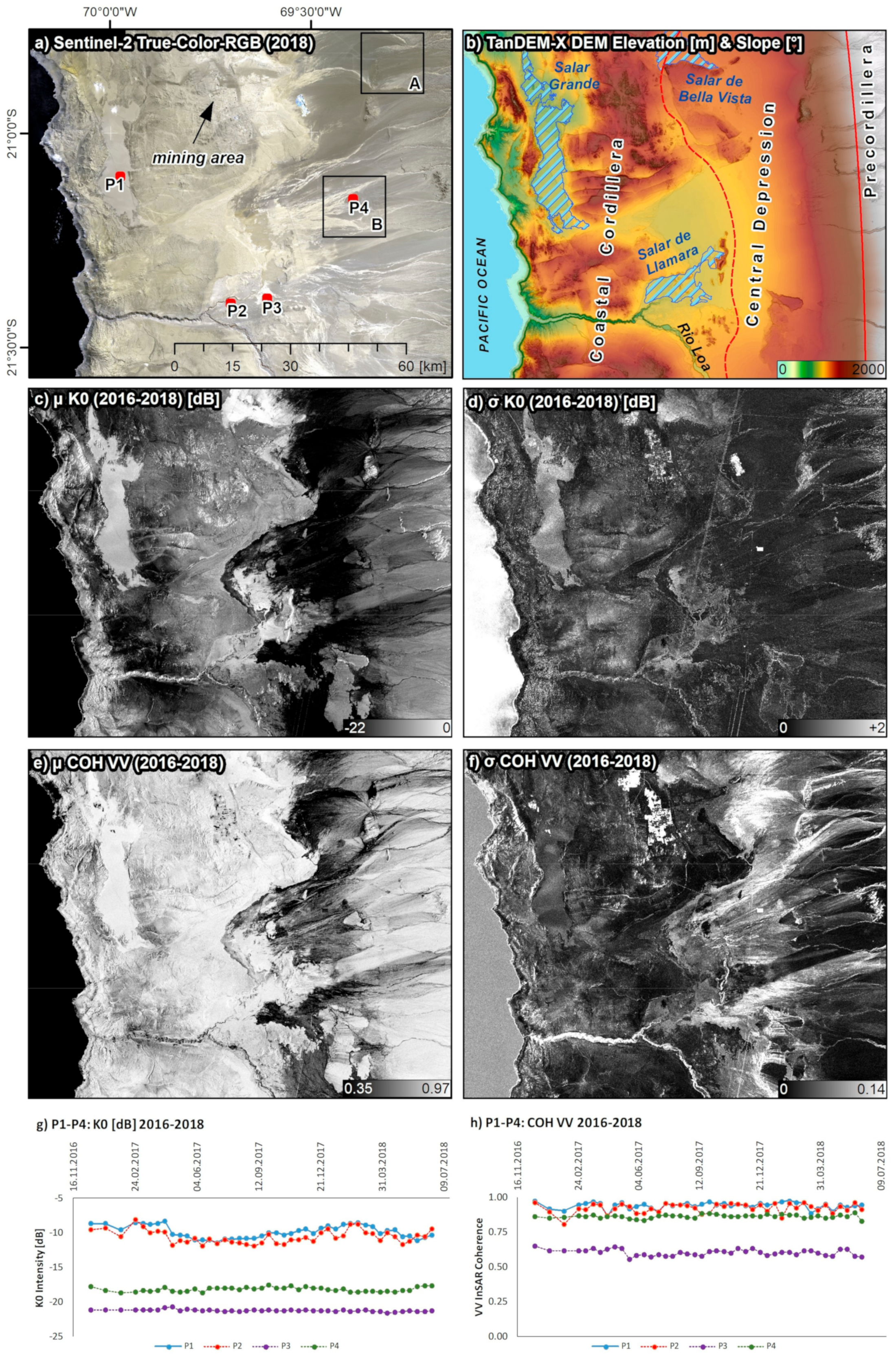
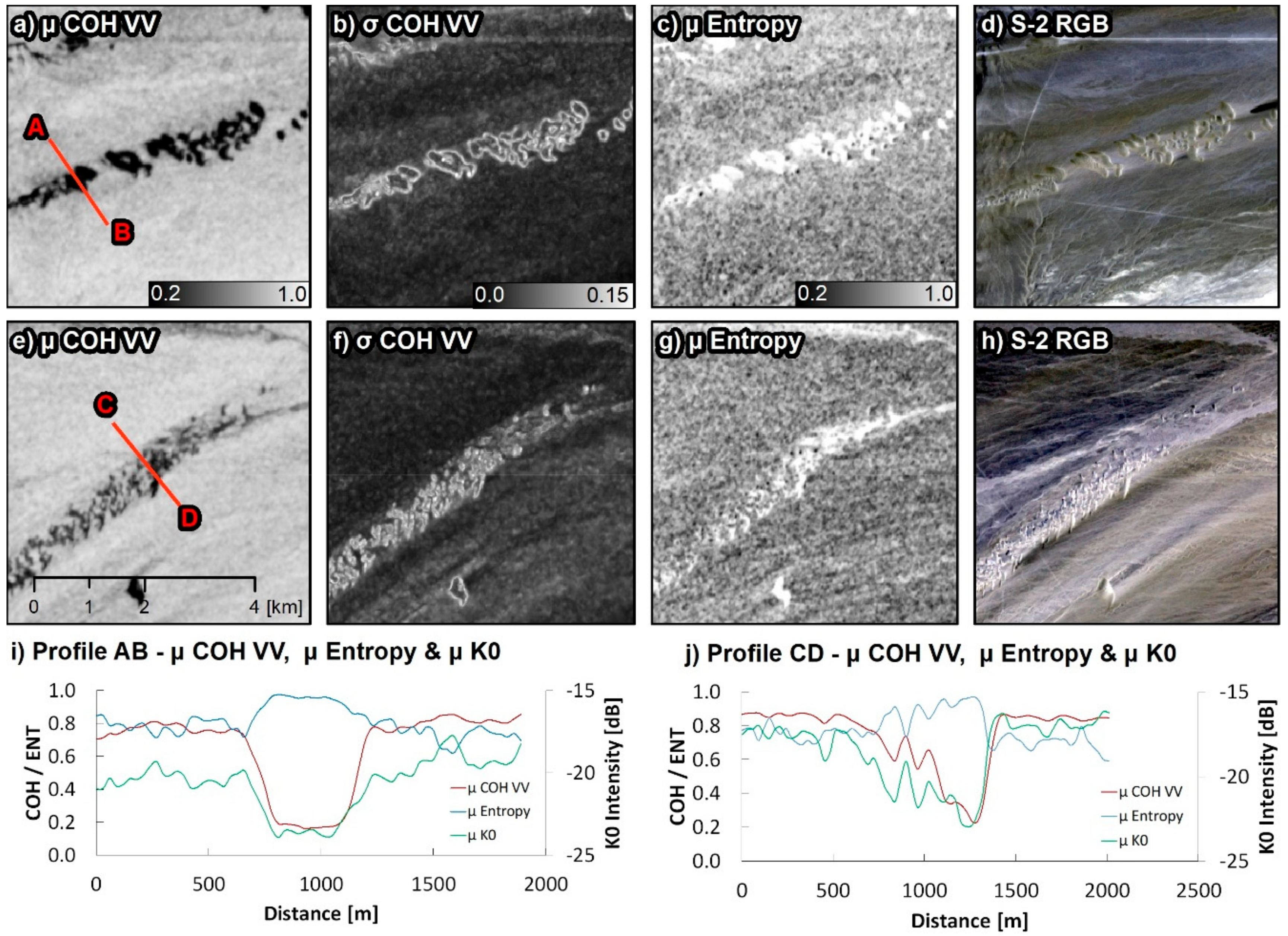
3.2.1. Relation of SAR Time Series Features to Geomorphic Domains
3.2.2. Influence of the Acquisition Geometry
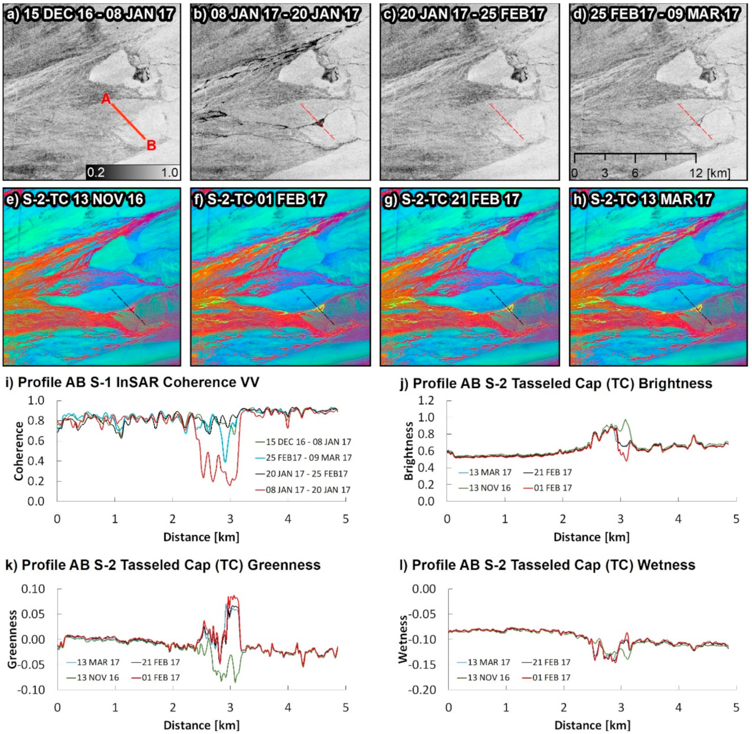
3.2.3. Relation of InSAR Coherence to SAR/DEM Features
4. Discussion
4.1. Long Temporal Baseline Mosaics
4.2. Short Temporal Baseline Time Series
5. Conclusions
Author Contributions
Funding
Acknowledgments
Conflicts of Interest
References
- European Space Agency (ESA). Sentinel-1 ESA’s Radar Observatory Mission for GMES Operational Services 2012; SP-1322/1; ESA Communications: Oakville, ON, Canada, 2012; pp. 1–88. [Google Scholar]
- European Space Agency (ESA). Mission Requirements Document for the European Radar Observatory Sentinel-1; ES-RS-ESA-SY-0007; European Space Agency: Paris, France, 2005; Volume 1, pp. 1–31. [Google Scholar]
- Di Traglia, F.; Nolesini, T.; Ciampalini, A.; Solari, L.; Frodella, W.; Bellotti, F.; Fumagalli, A.; De Rosa, G.; Casagli, N. Tracking morphological changes and slope instability using spaceborne and ground-based SAR data. Geomorphology 2018, 300, 95–112. [Google Scholar] [CrossRef]
- Ichoku, C.; Karnieli, A.; Arkin, Y.; Chorowicz, J.; Fleury, T.; Rudant, J.-P. Exploring the utility potential of SAR interferometric coherence images. Int. J. Remote Sens. 1998, 19, 1147–1160. [Google Scholar] [CrossRef]
- Touzi, R.; Lopes, A.; Bruniquel, J.; Vachon, P.W. Coherence estimation for SAR imagery. IEEE Trans. Geosci. Remote Sens. 1999, 37, 135–149. [Google Scholar] [CrossRef] [Green Version]
- Monti-Guarnieri, A.V.; Brovelli, M.A.; Manzoni, M.; d’Alessandro, M.M.; Molinari, M.E.; Oxoli, D. Coherent change detection for multipass SAR. IEEE Trans. Geosci. Remote Sens. 2018, 56, 6811–6822. [Google Scholar] [CrossRef]
- Scheuchl, B.; Ullmann, T.; Koudogbo, F. Change Detection using high resolution TerraSAR-X data preliminary results. In Proceedings of the ISPRS Hannover Workshop, Hannover, Germany, 2–5 June 2009; pp. 1–4. [Google Scholar]
- Ullmann, T.; Serfas, K.; Büdel, C.; Padashi, M.; Baumhauer, R. Data processing, feature extraction, and time-series analysis of Sentinel-1 synthetic aperture radar (SAR) imagery: Examples from damghan and bajestan playa (Iran). Zeitschrift für Geomorphologie 2019, 62, 9–39. [Google Scholar] [CrossRef]
- Zebker, H.A.; Villasenor, J. Decorrelation in interferometric radar echoes. IEEE Trans. Geosci. Remote Sens. 1992, 30, 950–959. [Google Scholar] [CrossRef] [Green Version]
- Plank, S. Rapid damage assessment by means of multi-temporal SAR—A comprehensive review and outlook to Sentinel-1. Remote Sens. 2014, 6, 4870–4906. [Google Scholar] [CrossRef] [Green Version]
- Oxoli, D.; Boccardo, P.; Brovelli, M.A.; Molinari, M.E.; Monti Guarnieri, A. Coherent change detection for repeated-pass interferometric SAR images: An application to earthquake damage assessment on buildings. In Proceedings of the ISPRS-International Archives of the Photogrammetry, Remote Sensing and Spatial Information Sciences; Copernicus GmbH: Göttingen, Germany, 2018; Volume XLII-3-W4, pp. 383–388. [Google Scholar]
- Washaya, P.; Balz, T.; Mohamadi, B. Coherence change-detection with Sentinel-1 for natural and anthropogenic disaster monitoring in urban areas. Remote Sens. 2018, 10, 1026. [Google Scholar] [CrossRef] [Green Version]
- Wegmuller, U.; Strozzi, T.; Farr, T.; Werner, C.L. Arid land surface characterization with repeat-pass SAR interferometry. IEEE Trans. Geosci. Remote Sens. 2000, 38, 776–781. [Google Scholar] [CrossRef]
- Liu, J.G.; Black, A.; Lee, H.; Hanaizumi, H.; Moore, J.M. Land surface change detection in a desert area in Algeria using multi-temporal ERS SAR coherence images. Int. J. Remote Sens. 2001, 22, 2463–2477. [Google Scholar] [CrossRef]
- Catherine, B.; André, O. The use of SAR interferometric coherence images to study sandy desertification in southeast Niger: Preliminary results. In Proceedings of the Envisat Symposium 2007, Montreux, Switzerland, 23–27 April 2007; pp. 1–5. [Google Scholar]
- Oyen, A.M.; Koenders, R.; Aria, S.E.H.; Lindenbergh, R.C.; Li, J.; Donselaar, M.E. Application of synthetic aperture radar methods for morphological analysis of the Salar De Uyuni distal fluvial system. In Proceedings of the 2012 IEEE International Geoscience and Remote Sensing Symposium, Munich, Germany, 22–27 July 2012; pp. 3875–3878. [Google Scholar]
- Gaber, A.; Abdelkareem, M.; Abdelsadek, I.S.; Koch, M.; El-Baz, F. Using InSAR coherence for investigating the interplay of fluvial and aeolian features in arid lands: Implications for groundwater potential in Egypt. Remote Sens. 2018, 10, 832. [Google Scholar] [CrossRef] [Green Version]
- Ullmann, T.; Büdel, C.; Baumhauer, R.; Padashi, M. Sentinel-1 SAR data revealing fluvial morphodynamics in damghan (Iran): Amplitude and coherence change detection. Int. J. Earth Sci. Geophys. 2016, 2, 1–14. [Google Scholar] [CrossRef] [Green Version]
- Scott, C.P.; Lohman, R.B.; Jordan, T.E. InSAR constraints on soil moisture evolution after the March 2015 extreme precipitation event in Chile. Sci. Rep. 2017, 7, 4903. [Google Scholar] [CrossRef] [PubMed]
- Houston, J.; Hartley, A.J. The central Andean west-slope rainshadow and its potential contribution to the origin of hyper-aridity in the Atacama Desert. Int. J. Climatol. 2003, 23, 1453–1464. [Google Scholar] [CrossRef]
- Hartley, A.J.; Chong, G.; Houston, J.; Mather, A.E. 150 million years of climatic stability: Evidence from the Atacama Desert, northern Chile. J. Geol. Soc. 2005, 162, 421–424. [Google Scholar] [CrossRef]
- Rundel, P.; Dillon, M.; Palma, B.; Mooney, H.; Gulmon, S.; Ehleringer, J. The phytogeography and ecology of the coastal Atacama and Peruvian deserts. Aliso J. Syst. Evol. Bot. 1991, 13, 1–49. [Google Scholar] [CrossRef] [Green Version]
- Dunai, T.J.; López, G.A.G.; Juez-Larré, J. Oligocene–Miocene age of aridity in the Atacama Desert revealed by exposure dating of erosion-sensitive landforms. Geology 2005, 33, 321–324. [Google Scholar] [CrossRef]
- Rech, J.A.; Currie, B.S.; Shullenberger, E.D.; Dunagan, S.P.; Jordan, T.E.; Blanco, N.; Tomlinson, A.J.; Rowe, H.D.; Houston, J. Evidence for the development of the Andean rain shadow from a Neogene isotopic record in the Atacama Desert, Chile. Earth Planet. Sci. Lett. 2010, 292, 371–382. [Google Scholar] [CrossRef]
- de Porras, M.E.; Maldonado, A.; De Pol-Holz, R.; Latorre, C.; Betancourt, J.L. Late Quaternary environmental dynamics in the Atacama Desert reconstructed from rodent midden pollen records. J. Quat. Sci. 2017, 32, 665–684. [Google Scholar] [CrossRef]
- Cereceda, P.; Larrain, H.; Osses, P.; Farías, M.; Egaña, I. The spatial and temporal variability of fog and its relation to fog oases in the Atacama Desert, Chile. Atmos. Res. 2008, 87, 312–323. [Google Scholar] [CrossRef]
- del Río, C.G.; Rivera, D.S.; Siegmund, A.; Wolf, N.; Cereceda, P.; Larraín, H.; Lobos, F.; Garcia, J.L.; Osses, P.; Zanetta, N.; et al. ENSO influence on coastal fog-water yield in the Atacama Desert, Chile. Aerosol Air Qual. Res. 2018, 18, 127–144. [Google Scholar] [CrossRef] [Green Version]
- Cereceda, P.; Osses, P.; Larrain, H.; Farías, M.; Lagos, M.; Pinto, R.; Schemenauer, R.S. Advective, orographic and radiation fog in the Tarapacá region, Chile. Atmos. Res. 2002, 64, 261–271. [Google Scholar] [CrossRef]
- Clarke, J.D.A. Antiquity of aridity in the Chilean Atacama Desert. Geomorphology 2006, 73, 101–114. [Google Scholar] [CrossRef]
- Matmon, A.; Quade, J.; Placzek, C.; Fink, D.; Arnold, M.; Aumaître, G.; Bourlès, D.; Keddadouche, K.; Copeland, A.; Neilson, J.W. Seismic origin of the Atacama Desert boulder fields. Geomorphology 2015, 231, 28–39. [Google Scholar] [CrossRef]
- Owen, J.J.; Dietrich, W.E.; Nishiizumi, K.; Chong, G.; Amundson, R. Zebra stripes in the Atacama Desert: Fossil evidence of overland flow. Geomorphology 2013, 182, 157–172. [Google Scholar] [CrossRef]
- Wilcox, A.C.; Escauriaza, C.; Agredano, R.; Mignot, E.; Zuazo, V.; Otárola, S.; Castro, L.; Gironás, J.; Cienfuegos, R.; Mao, L. An integrated analysis of the March 2015 Atacama floods. Geophys. Res. Lett. 2016, 43, 8035–8043. [Google Scholar] [CrossRef]
- Jordan, T.E.; Herrera, C.; Godfrey, L.V.; Colucci, S.J.; Gamboa, C.; Urrutia, J.; González, G.; Paul, J.F. Isotopic characteristics and paleoclimate implications of the extreme precipitation event of March 2015 in northern Chile. Andean Geol. 2018, 46, 1–31. [Google Scholar] [CrossRef]
- Rech, J.A.; Quade, J.; Hart, W.S. Isotopic evidence for the source of Ca and S in soil gypsum, anhydrite and calcite in the Atacama Desert, Chile. Geochim. Cosmochim. Acta 2003, 67, 575–586. [Google Scholar] [CrossRef]
- Michalski, G.; Böhlke, J.K.; Thiemens, M. Long term atmospheric deposition as the source of nitrate and other salts in the Atacama Desert, Chile: New evidence from mass-independent oxygen isotopic compositions. Geochim. Cosmochim. Acta 2004, 68, 4023–4038. [Google Scholar] [CrossRef]
- Ewing, S.A.; Sutter, B.; Owen, J.; Nishiizumi, K.; Sharp, W.; Cliff, S.S.; Perry, K.; Dietrich, W.; McKay, C.P.; Amundson, R. A threshold in soil formation at Earth’s arid–hyperarid transition. Geochim. Cosmochim. Acta 2006, 70, 5293–5322. [Google Scholar] [CrossRef]
- Wang, F.; Michalski, G.; Luo, H.; Caffee, M. Role of biological soil crusts in affecting soil evolution and salt geochemistry in hyper-arid Atacama Desert, Chile. Geoderma 2017, 307, 54–64. [Google Scholar] [CrossRef]
- Abele, G. Salzkrusten, salzbedingte Solifluktion und Steinsalzkarst in der nordchilenisch-peruanischen Wüste. Mainz. Geogr. Stud. 1990, 34, 23–46. [Google Scholar]
- Quade, J.; Reiners, P.; Placzek, C.; Matmon, A.; Pepper, M.; Ojha, L.; Murray, K. Seismicity and the strange rubbing boulders of the Atacama Desert, northern Chile. Geology 2012, 40, 851–854. [Google Scholar] [CrossRef]
- May, S.M.; Hoffmeister, D.; Wolf, D.; Bubenzer, O. Zebra stripes in the Atacama Desert revisited—Granular fingering as a mechanism for zebra stripe formation? Geomorphology 2019, 344, 46–59. [Google Scholar] [CrossRef]
- Cloude, S.R.; Pottier, E. A review of target decomposition theorems in radar polarimetry. IEEE Trans. Geosci. Remote Sens. 1996, 34, 498–518. [Google Scholar] [CrossRef]
- Cloude, S. The dual polarisation entropy/alpha decomposition: A PALSAR case study. In Proceedings of the 3rd International Workshop on Science and Applications of SAR Polarimetry and Polarimetric Interferom, Frascati, Italy, 22–26 January 2007; pp. 1–6. [Google Scholar]
- Schmitt, A.; Wendleder, A.; Hinz, S. The Kennaugh element framework for multi-scale, multi-polarized, multi-temporal and multi-frequency SAR image preparation. ISPRS J. Photogramm. Remote Sens. 2015, 102, 122–139. [Google Scholar] [CrossRef] [Green Version]
- Zhang, Z.; Wang, C.; Zhang, H.; Tang, Y.; Liu, X. Analysis of permafrost region coherence variation in the Qinghai–Tibet plateau with a high-resolution TerraSAR-X image. Remote Sens. 2018, 10, 298. [Google Scholar] [CrossRef] [Green Version]
- Mullissa, A.; Tolpekin, V.; Stein, A.; Perissin, D. Polarimetric differential SAR interferometry in an arid natural environment. Int. J. Appl. Earth Obs. Geoinf. 2017, 59, 9–18. [Google Scholar] [CrossRef]
- Thomas, K. The tasselled cap—A graphic description of the spectral-temporal development of agricultural crops as seen by Landsat. In Proceedings of the Symposium on Machine Processing of Remotely Sensed Data, West Lafayette, IN, USA, 29 June–1 July 1976; pp. 1–11. [Google Scholar]
- Kauth, C. The tasseled cap de-mystified. Transformations of MSS and TM data. Photogramm. Eng. Remote Sens. 1986, 52, 81–86. [Google Scholar]
- Bozkurt, D.; Rondanelli, R.; Garreaud, R.; Arriagada, A. Impact of warmer eastern tropical pacific SST on the March 2015 Atacama floods. Mon. Weather Rev. 2016, 144, 4441–4460. [Google Scholar] [CrossRef] [Green Version]
- European Space Agency (ESA). Sentinel-2 User Handbook; European Space Agency: Paris, France, 2015; pp. 1–64. [Google Scholar]
- European Space Agency (ESA). S2 MPC Sen2Cor Software Release Note; S2-PDGS-MPC-L2A-SRN-V2.8.0; European Space Agency: Paris, France, 2019; Volume 2, pp. 1–77. [Google Scholar]
- Deutsches Zentrum für Luft-und Raumfahrt (DLR). TanDEM-X Ground Segment DEM Products Specification Document; TD-GS-PS-0021; Deutsches Zentrum für Luft-und Raumfahrt: Cologne, Germany, 2016; pp. 1–46. [Google Scholar]
- Gruber, A.; Wessel, B.; Huber, M.; Roth, A. Operational TanDEM-X DEM calibration and first validation results. ISPRS J. Photogramm. Remote Sens. 2012, 73, 39–49. [Google Scholar] [CrossRef]
- Gonzalez, C.; Braeutigam, B.; Martone, M.; Rizzoli, P. Relative height error estimation method for TanDEM-X DEM products. In Proceedings of the EUSAR 2014; 10th European Conference on Synthetic Aperture Radar, Berlin, Germany, 3–5 June 2014; pp. 1–4. [Google Scholar]
- Pipaud, I.; Loibl, D.; Lehmkuhl, F. Evaluation of TanDEM-X elevation data for geomorphological mapping and interpretation in high mountain environments—A case study from SE Tibet, China. Geomorphology 2015, 246, 232–254. [Google Scholar] [CrossRef]
- Ullmann, T.; Büdel, C.; Baumhauer, R. Characterization of arctic surface morphology by means of intermediated TanDEM-X digital elevation model data. Zeitschrift für Geomorphologie Supplementary Issues 2017, 61, 3–25. [Google Scholar] [CrossRef]
- Kramm, T.; Hoffmeister, D. A relief dependent evaluation of digital elevation models on different scales for northern Chile. ISPRS Int. J. Geo Inf. 2019, 8, 430. [Google Scholar] [CrossRef] [Green Version]
- Gruber, S.; Peckham, S. Chapter 7 land-surface parameters and objects in hydrology. In Developments in Soil Science; Geomorphometry; Hengl, T., Reuter, H.I., Eds.; Elsevier: Amsterdam, The Netherlands, 2009; Volume 33, pp. 171–194. [Google Scholar]
- Pelletier, J.D. Quantitative Modeling of Earth Surface Processes; Cambridge University Press: Cambridge, UK, 2008. [Google Scholar]
- Segerstrom, K. Quaternary geology of Chile: Brief outline. Geol. Soc. Am. Bull. 1964, 75, 157. [Google Scholar] [CrossRef]
- May, S.M.; Meine, L.; Hoffmeister, D.; Brill, D.; Medialdea, A.; Wennrich, V.; Gröbner, M.; Schulte, P.; Steininger, F.; Deprez, M.; et al. Origin and timing of past hillslope activity in the hyper-arid core of the Atacama Desert—The formation of fine sediment lobes along the chuculay fault system, Northern Chile. Glob. Planet. Chang. 2019, 184, 103057. [Google Scholar] [CrossRef]


| DEM | Slope | TWI | µ K0 | σ K0 | µ Entropy | σ Entropy | µ COH VV | σ COH VV | µ COH VH | σ COH VH | |
|---|---|---|---|---|---|---|---|---|---|---|---|
| DEM | 1.00 | 0.53 | −0.58 | 0.41 | 0.28 | −0.19 | 0.08 | 0.14 | 0.22 | 0.23 | 0.25 |
| Slope | 0.53 | 1.00 | −0.69 | 0.49 | 0.42 | −0.14 | 0.09 | 0.05 | 0.42 | 0.28 | 0.35 |
| TWI | −0.58 | −0.69 | 1.00 | −0.36 | −0.25 | 0.21 | 0.03 | −0.22 | −0.10 | −0.33 | −0.16 |
| µ K0 | 0.41 | 0.49 | −0.36 | 1.00 | 0.47 | −0.37 | 0.09 | 0.65 | 0.07 | 0.84 | 0.13 |
| σ K0 | 0.28 | 0.42 | −0.25 | 0.47 | 1.00 | −0.21 | 0.40 | 0.05 | 0.39 | 0.25 | 0.38 |
| µ Entropy | −0.19 | −0.14 | 0.21 | −0.37 | −0.21 | 1.00 | −0.33 | −0.47 | 0.08 | −0.21 | −0.33 |
| σ Entropy | 0.08 | 0.09 | 0.03 | 0.09 | 0.40 | −0.33 | 1.00 | −0.01 | 0.25 | −0.09 | 0.41 |
| µ COH VV | 0.14 | 0.05 | −0.22 | 0.65 | 0.05 | −0.47 | −0.01 | 1.00 | −0.55 | 0.80 | −0.17 |
| σ COH VV | 0.22 | 0.42 | −0.10 | 0.07 | 0.39 | 0.08 | 0.25 | −0.55 | 1.00 | −0.23 | 0.65 |
| µ COH VH | 0.23 | 0.28 | −0.33 | 0.84 | 0.25 | −0.21 | −0.09 | 0.80 | −0.23 | 1.00 | −0.18 |
| σ COH VH | 0.25 | 0.35 | −0.16 | 0.13 | 0.38 | −0.33 | 0.41 | −0.17 | 0.65 | −0.18 | 1.00 |
© 2019 by the authors. Licensee MDPI, Basel, Switzerland. This article is an open access article distributed under the terms and conditions of the Creative Commons Attribution (CC BY) license (http://creativecommons.org/licenses/by/4.0/).
Share and Cite
Ullmann, T.; Sauerbrey, J.; Hoffmeister, D.; May, S.M.; Baumhauer, R.; Bubenzer, O. Assessing Spatiotemporal Variations of Sentinel-1 InSAR Coherence at Different Time Scales over the Atacama Desert (Chile) between 2015 and 2018. Remote Sens. 2019, 11, 2960. https://doi.org/10.3390/rs11242960
Ullmann T, Sauerbrey J, Hoffmeister D, May SM, Baumhauer R, Bubenzer O. Assessing Spatiotemporal Variations of Sentinel-1 InSAR Coherence at Different Time Scales over the Atacama Desert (Chile) between 2015 and 2018. Remote Sensing. 2019; 11(24):2960. https://doi.org/10.3390/rs11242960
Chicago/Turabian StyleUllmann, Tobias, Julia Sauerbrey, Dirk Hoffmeister, Simon Matthias May, Roland Baumhauer, and Olaf Bubenzer. 2019. "Assessing Spatiotemporal Variations of Sentinel-1 InSAR Coherence at Different Time Scales over the Atacama Desert (Chile) between 2015 and 2018" Remote Sensing 11, no. 24: 2960. https://doi.org/10.3390/rs11242960