Evaluating Combinations of Sentinel-2 Data and Machine-Learning Algorithms for Mangrove Mapping in West Africa


1
Department of Geography and Spatial Sciences, University of Delaware, Newark, DE 19716, USA
2
Department of Plant and Soil Sciences, University of Delaware, Newark, DE 19716, USA
3
Center for International Earth Science Information Network (CIESIN), Columbia University, Palisades, NY 10964, USA
4
The Center for Geographic Analysis (CGA), Harvard University, Cambridge, MA 02138, USA
5
NASA Goddard Space Flight Center, Greenbelt, MD 20771, USA
6
Department of Coastal Studies, East Carolina University, Wanchese, NC 27948, USA
*
Author to whom correspondence should be addressed.
Remote Sens. 2019, 11(24), 2928; https://doi.org/10.3390/rs11242928
Submission received: 1 October 2019
/
Revised: 21 November 2019
/
Accepted: 3 December 2019
/
Published: 6 December 2019
(This article belongs to the Special Issue EO Solutions to Support Countries Implementing the SDGs)
Abstract
:Creating a national baseline for natural resources, such as mangrove forests, and monitoring them regularly often requires a consistent and robust methodology. With freely available satellite data archives and cloud computing resources, it is now more accessible to conduct such large-scale monitoring and assessment. Yet, few studies examine the reproducibility of such mangrove monitoring frameworks, especially in terms of generating consistent spatial extent. Our objective was to evaluate a combination of image processing approaches to classify mangrove forests along the coast of Senegal and The Gambia. We used freely available global satellite data (Sentinel-2), and cloud computing platform (Google Earth Engine) to run two machine learning algorithms, random forest (RF), and classification and regression trees (CART). We calibrated and validated the algorithms using 800 reference points collected using high-resolution images. We further re-ran 10 iterations for each algorithm, utilizing unique subsets of the initial training data. While all iterations resulted in thematic mangrove maps with over 90% accuracy, the mangrove extent ranges between 827–2807 km2 for Senegal and 245–1271 km2 for The Gambia with one outlier for each country. We further report “Places of Agreement” (PoA) to identify areas where all iterations for both methods agree (506.6 km2 and 129.6 km2 for Senegal and The Gambia, respectively), thus have a high confidence in predicting mangrove extent. While we acknowledge the time- and cost-effectiveness of such methods for the landscape managers, we recommend utilizing them with utmost caution, as well as post-classification on-the-ground checks, especially for decision making.
Keywords:
mangrove; machine-learning algorithms; google earth engine; random forest; CART; Senegal; The Gambia; Africa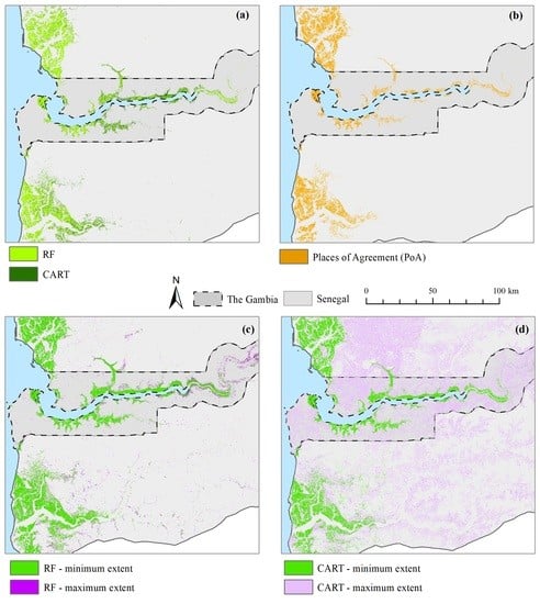
1. Introduction
Mangrove forests cover approximately 0.7% of tropical forest area around the world [1,2,3,4], in more than 118 tropical and sub-tropical countries. Yet, these forests can store three to four times more carbon per equivalent area compared to tropical forests [5]. In particular, mangrove forests in carbonate, peat-dominated settings are likely to store 25–50% more soil organic carbon compared to mangroves in deltaic and estuarine coastal settings [6]. These forests are also known to host 1.6% of the total tropical forest biomass (considering both above- and below-ground biomass) [7].
In Africa, mangrove forests covered approximately 27,465 km2 in 2010 [1] and provide important ecosystem services to vulnerable coastal population, including protection from storm surges, reduction of coastal erosion, water quality, alternate livelihood, etc. [8,9,10,11,12]. However, studies monitoring mangroves in Africa are unevenly distributed in space and time. Several studies documented mangrove extent or changes across Africa [13,14,15,16,17,18,19,20,21,22,23,24,25,26,27], but primarily focusing on a few countries, such as Gambia, Guinea-Bissau, Guinea, Mauritania, Mozambique, Madagascar, Nigeria, Senegal, Sierra Leone, South Africa, and Tanzania. Moreover, most studies do not cover a temporal span suitable for longer-term consistent monitoring, such as those useful for tracking the sustainable development goals (SDG) adopted by the United Nations, especially Goal 15 (‘Life on Land’) indicator 15.1.1 for quantifying “forest area as a proportion of total land area”.
Remote sensing provides a time- and cost-effective approach for natural resource monitoring at any large scale, especially at the national level. Particularly for mangrove mapping, remote sensing methods have been widely used [13,14,15,16,17,18,19,20,21,22,23,24,25,26,27,28,29,30,31,32,33,34,35,36,37,38,39,40,41,42,43,44,45,46,47,48,49,50,51,52,53,54,55,56,57]. Most of these studies use optical satellite data, especially Landsat, due to longer temporal coverage and ease of data accessibility. With the availability of active satellite data, many studies are increasingly utilizing radar data from sensors including the Advanced Land Observing Satellite (ALOS) based Phased Array type L-band Synthetic Aperture Radar (ALOS PALSAR), RADARSAT-2, the Shuttle Radar Topography Mission (SRTM), for quantifying mangrove extent and other biophysical characteristics [15,58,59,60,61,62,63,64,65]. While availability of Sentinel-1 from the European Space Agency (ESA) data has shown promise for continued use of radar data in mangrove mapping in the coming years, historical land cover mapping and monitoring often need to rely solely on optical remote sensing data due to the lack of radar data before the 1990s.
In terms of the methods, prior studies use a range of classification techniques such as the iterative self-organizing data analysis (ISODATA) clustering, maximum likelihood classification (MLC), hybrid, random forest (RF), classification and regression trees (CART), support vector machine (SVM), and object oriented classification among others [16,17,34,37,38,39,40,41,43,66]. With the advent of cloud computing platforms with free access to petabytes of geospatial data, such as Google Earth Engine (GEE), it has now become increasingly accessible and straight-forward to analyze enormous amounts of satellite imagery covering large regions [37,67,68,69,70,71,72]. While GEE offers more than 15 classification techniques, most studies rely on machine-learning algorithms [37,68,69,70,71,72], such as CART and RF, since these have proven to be some of the robust methods for land cover classifications. Such methods based on free data and robust algorithms can be particularly beneficial for regular monitoring, including tracking SDG indicators.
Landscape managers in many developing countries struggle to establish a consistent methodology for SDG monitoring and assessments, both spatial and temporal. This is primarily due to the lack of computing resources required for method development using high-resolution satellite data, limited accessibility to high-resolution satellite data, and challenging physical environment for collecting data required for method calibration and validation. Such systematic monitoring is even more challenging for wetland forests due to the difficult terrain and often remote location. While significant advances have been achieved in satellite-derived monitoring in the recent past, few studies focus on the ease of the landscape managers to adopt the methodology for on-the-ground monitoring, and evaluate the performance of machine-learning algorithms in identifying mangrove extent in fragmented, heterogeneous, and rapidly changing landscapes. In this study, our objective is to evaluate freely available satellite data and machine-learning algorithms, specifically RF and CART, available on GEE to predict mangrove extent in the West African countries of Senegal and The Gambia. We evaluated the performance of these two classifiers by running 10 iterations for each, using Sentinel-2 images for 2017 and comparing the range of mangrove extent and accuracy for each iteration. Our objective was to examine if a simple framework that relies on freely available geospatial resources can provide consistent and reliable mangrove estimates, rather than identifying the best model parameters to generate the most accurate land cover map for the study area.
2. Materials and Methods
2.1. Study Area
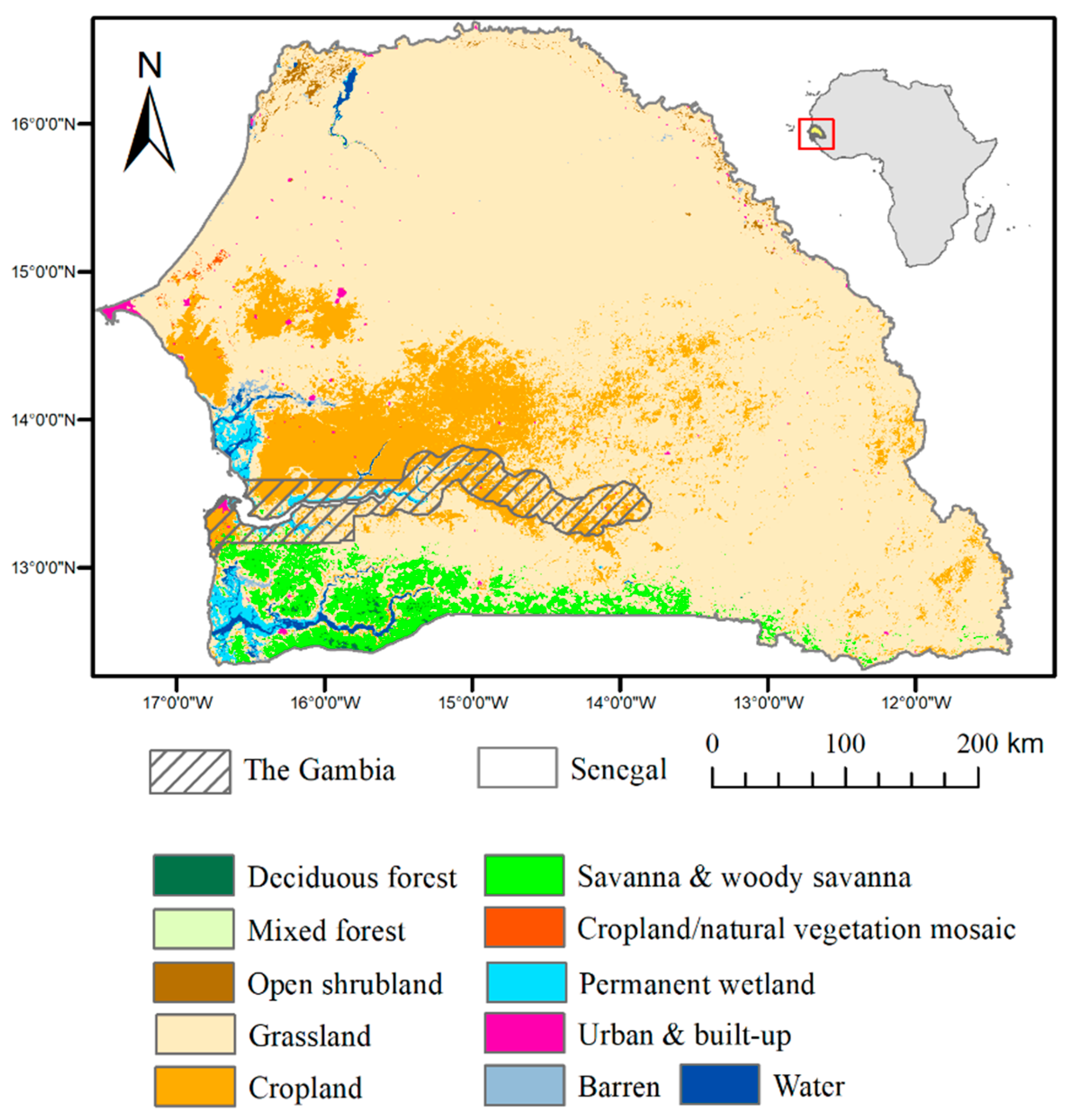
Senegal, covering a land area of 192,530 km2, is home to over 12.7 million people, out of which nearly two-thirds live in the coastal region. The country has a tropical climate and heavier vegetation in the southern part, whereas the northern part is dominated by the desert and grasslands influenced by a Sahelian climate (Figure 1) with projected changes in wet and dry extremes in the coming decades [73]. Approximately 70% of the population depends on agriculture that covers 46% of the land area [74], and is highly vulnerable to ongoing and future climate variability and change. The Gambia is the smallest country in mainland Africa, covering a land area of 10,120 km2. Other than permanent wetlands and grasslands, the country is dominated by croplands (Figure 1), covering approximately 60% of the land area [74]. Table 1 includes estimation of land cover types as extracted from MODIS land cover type global data product (MCD12Q1) [75].
The mangroves in this landscape are primarily located in the Sine-Saloum and Casamance Deltas, but smaller areas are also located near Dakar and in the northern end. The Sine-Saloum Delta is located north of The Gambia in the Sahelian climate zone with an average rainfall of 450–920 mm per year. The Casamance Delta is located south of The Gambia within the Sudanese–Guinean climate zone, with rainfall between 800 and 1700 mm per year. The region experiences monsoonal rainfall that occurs between June and September [76]. The coastal regions of Senegal experience microtidal (<2 m), semi-diurnal tides [77].
The region is dominated by two mangrove species. Rhizophora racemosa occur along the tidal channels while Avicennia germinans are generally located further from the channel in tidal flats that tend to have higher salinities [78]. More recently, R. mangle has been planted during large restoration efforts across the country at a density of 5000 stems per hectare [79]. Just landward of the mangrove margins are barren mud flats with high salinity, creating a distinct separation between the mangroves and upland vegetation [78]. Across the country, the mean mangrove height is 6.9 m with a maximum height of 11.9 m [80].
2.2. Satellite Data
We accessed Sentinel-2 level-1C assets on GEE provided by the European Space Agency (ESA). We used the top-of-atmosphere (TOA) reflectance data that included radiometric and geometric corrections following the methods described in the Sentinel-2 User Handbook [81]. Specifically, we used the GEE function “ee.ImageCollection” to filter the time-series data for the calendar year 2017 and considered all bands with spatial resolution 10 m and 20 m (bands 2–8a, 11,12). The TOA reflectance data used in this study generally retain considerable atmospheric signals. For studies considering biophysical properties of vegetation, TOA reflectance data should be corrected for atmospheric signals and the resulting surface reflectance data should be used. However, we converted TOA reflectance data into categorical land cover map (thematic information) in this study, hence our findings should not be influenced by our data choice. We then calculated the Normalized Difference Vegetation Index (NDVI) and added the NDVI band to each image. A total of 4153 images were considered for the study period and region, with cloud coverage ranging between 0–100% with an average of 34%. An annual composite was generated using a ‘quality mosaic’ that selected cloud-free greenest pixels [82,83,84]. In other words, the maximum NDVI values in the stack of pixels within entire time-series determined the rest of the reflectance band values in the annual composite in order to capture the vegetation pixels at the same phenological stage. This method was repeated for both Senegal and The Gambia. The quality mosaic served as the input image for the classifiers (Section 2.4).
2.3. Training and Testing the Classifiers
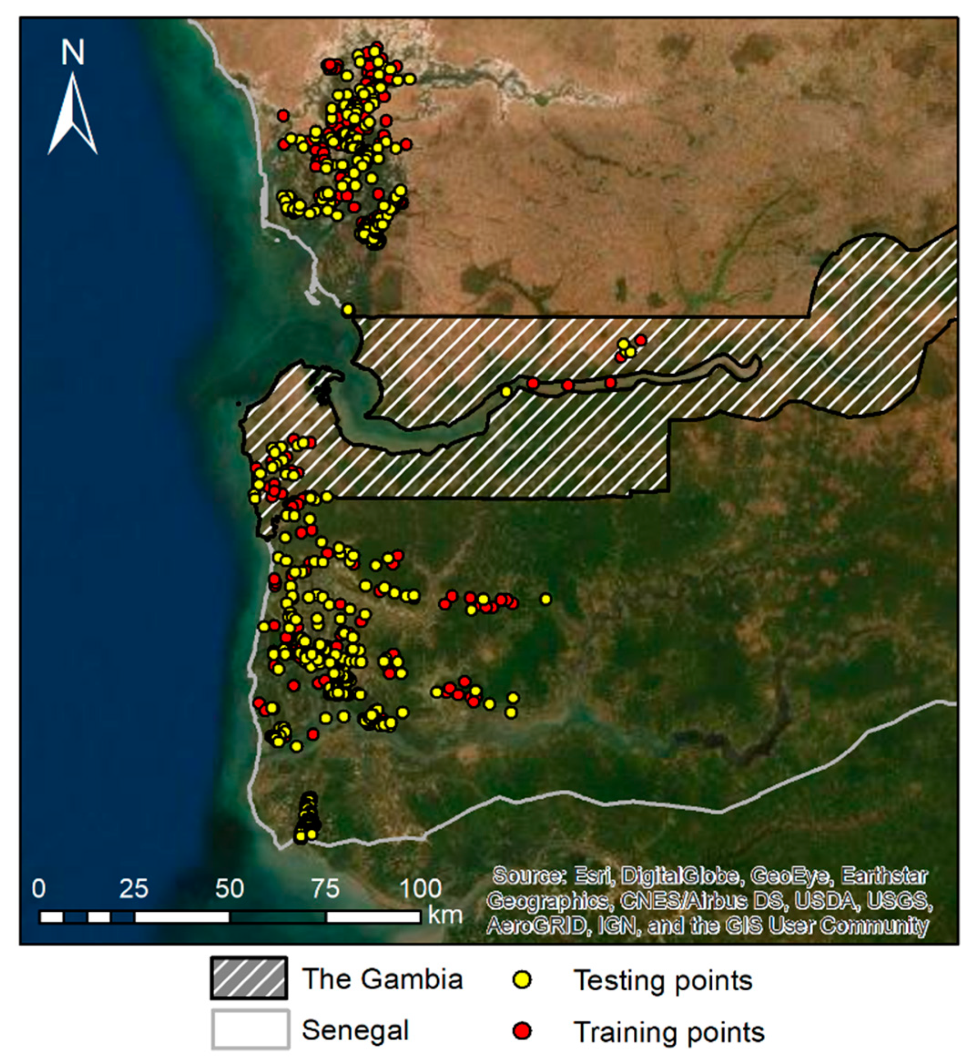
We collected a total of 800 reference points for the four land cover classes (mangrove, water, other vegetation, and sand/soil) for the Senegal–Gambia landscape (Figure 2). We used both high-resolution images available on GEE and the greenest-pixel composite to facilitate reference data collection. We considered homogeneous patches of a specific land cover (i.e., same land cover for at least 9 Sentinel-2 pixels) for collecting reference points. We avoided fragmented landscape to minimize mixed pixel issues, and/or to avoid collecting reference points from the edge of a particular land cover. For this reason, we have fewer points in The Gambia. However, the landscape was classified as a whole, and not for each country separately. Hence, fewer training points in The Gambia should not severely affect the outputs, as long as land covers have similar spectral signatures in both countries. We used a stratified random sampling approach based on a visual assessment of the relative proportion of different land covers in the coastal zone of the study area, and collected 500 points for the mangrove class, and 100 points for each of the other three land covers. We used half of the 800 points collected for training the classifiers (i.e., ‘train’ points on GEE), and the other half for accuracy assessment (i.e., ‘test’ points on GEE). We reported producer’s/user’s/overall accuracy as well as kappa (κ) coefficient [85]. Producer’s accuracy measures the error of omission, i.e., the proportion of pixels in a certain class that is being evaluated that were incorrectly classified in another category and were omitted from the ‘truth’ class as identified by the test points. User’s accuracy measures the error of commission, i.e., the proportion of pixels that were incorrectly included in a class that is being evaluated.
2.4. The Classifiers
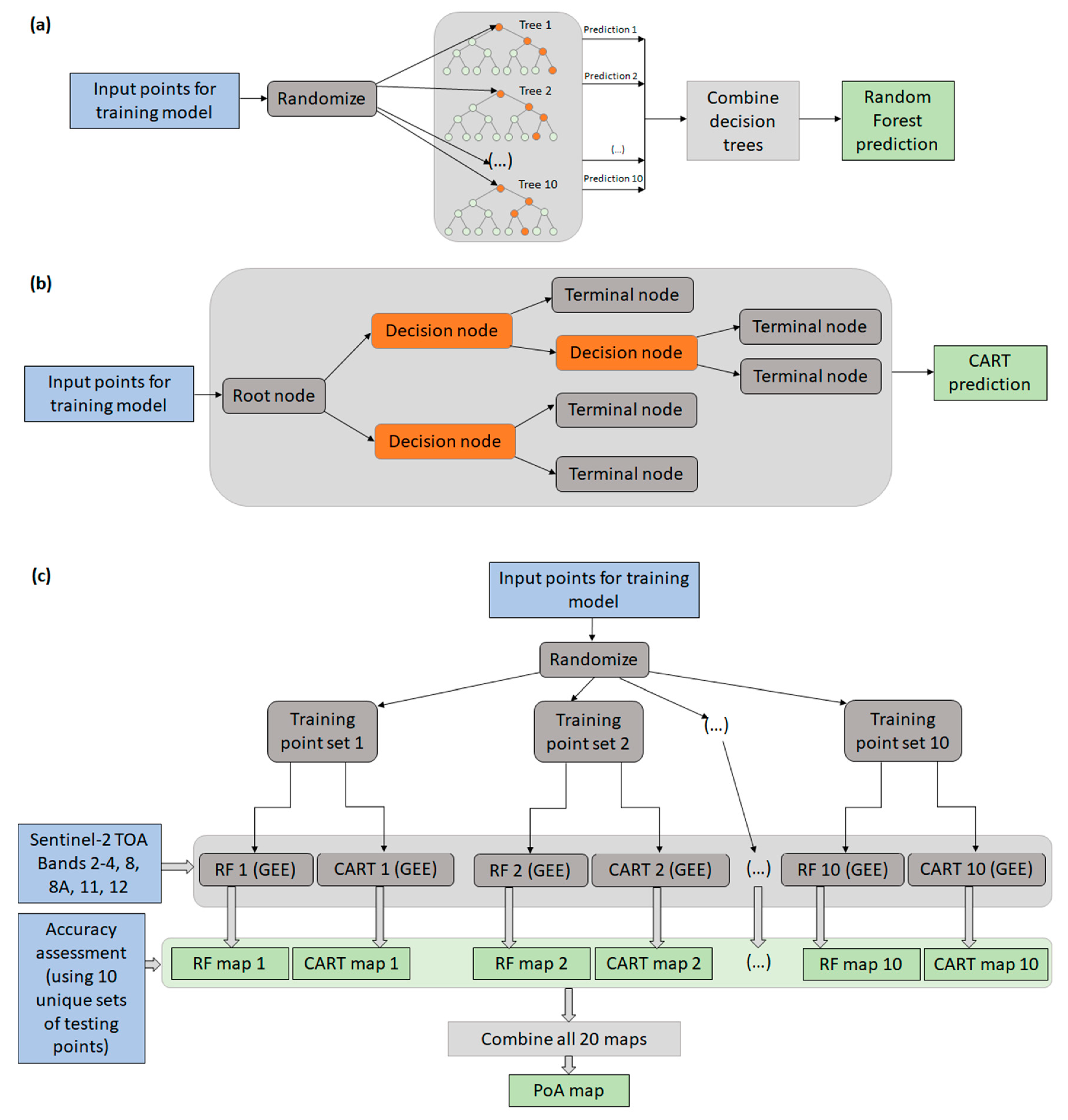
The RF is an ensemble of tree-based classifiers where each classifier uses a random vector sampled independently from the original training set (Figure 3a), and each tree casts a vote to the most popular class [87,88]. The RF uses ‘bootstrap aggregating’ or ‘bagging’ [78], a method to generate random vectors with replacement N examples (where N is the size of the original input training data), to select training data for each class. Each pixel is assigned to a class based on the most popular vote from all tree predictors (Figure 3a). The number of trees and variables per split in a RF classifier is defined by the user. Since the classifier performance is not sensitive to the number of variables per split [89], limiting this value to the square root of the input variables (a default value for RF in GEE and R statistical software) can help with reducing the computational complexity and decreasing correlation among the trees [89]. Unlike decision tree (DT) classifiers (such as CART), pruning is not required for RF. However, RF classifiers are more complex than DT classifiers, are less intuitive due to the inherent complexity, and can be computationally intensive. We used 10 trees and the square root of the number of inputs for variables per split in this study. Since the objective of this study is to evaluate the performance of machine-learning algorithms that can be easily reproducible in developing countries with limited computing resources, and not to find out the best parameters for these algorithms, we decided to generate simple yet robust models with the default parameters available on GEE.
The CART is a decision-rule based classifier that operates in a tree-structured decision space (Figure 3b) and is a modern-day analog to the DT approach [90]. Within CART, input data are recursively split at each decision node (Figure 3b), also known as a greedy splitting approach, based on a statistical test (such as Gini index) to increase the homogeneity of the training data in the resulting nodes. Since a complex tree runs the risk of overfitting, thus reducing the accuracy of the classified output, pruning the tree (i.e., removing the tree sections that do not contribute to increased accuracy) is an important step in a DT classifier. One known limitation of CART is high variance across samples leading to high variability in predicted classes and estimates [91]. For the CART classifiers used in this study, we have used the default values of 10 for both the cross-validation factor for pruning and maximum depth of the tree (i.e., maximum level that the initial tree can grow), in order to minimize the computational resource usage that is often a limitation in many developing countries. The standard error threshold of 0.5 was used to determine the simplest tree with an accuracy comparable to the minimum cost-complexity tree.
The output classified images for both classifiers have a spatial resolution of 20 m. We calculated the area under mangroves by multiplying the number of pixels classified as mangrove by the cell size. We further calculated area under the “places of agreement (PoA)” that were classified as mangrove pixels by both algorithms (Figure 3c). All output images were further clipped for low elevation coastal zone (LECZ) with elevation ≤40 m, a criterion widely used to define LECZ (e.g., see [16]). All analyses were performed using GEE and ArcMap 10.5.1.
2.5. Model Cross-Validation
For each of the two classifiers, we ran 10 iterations to determine the range of accuracies of the classified maps (Figure 3c). In order to do that, we randomly selected 400 training points for each iteration out of the 800 total points collected before running the classifiers using stratified random sampling in ArcMap 10.5.1 and trained the classifiers on GEE. In other words, we created a unique set of 400 points each for training and testing. We utilized the iteration-specific set for training and testing points for both classifiers.
3. Results
3.1. Accuracy Assessment
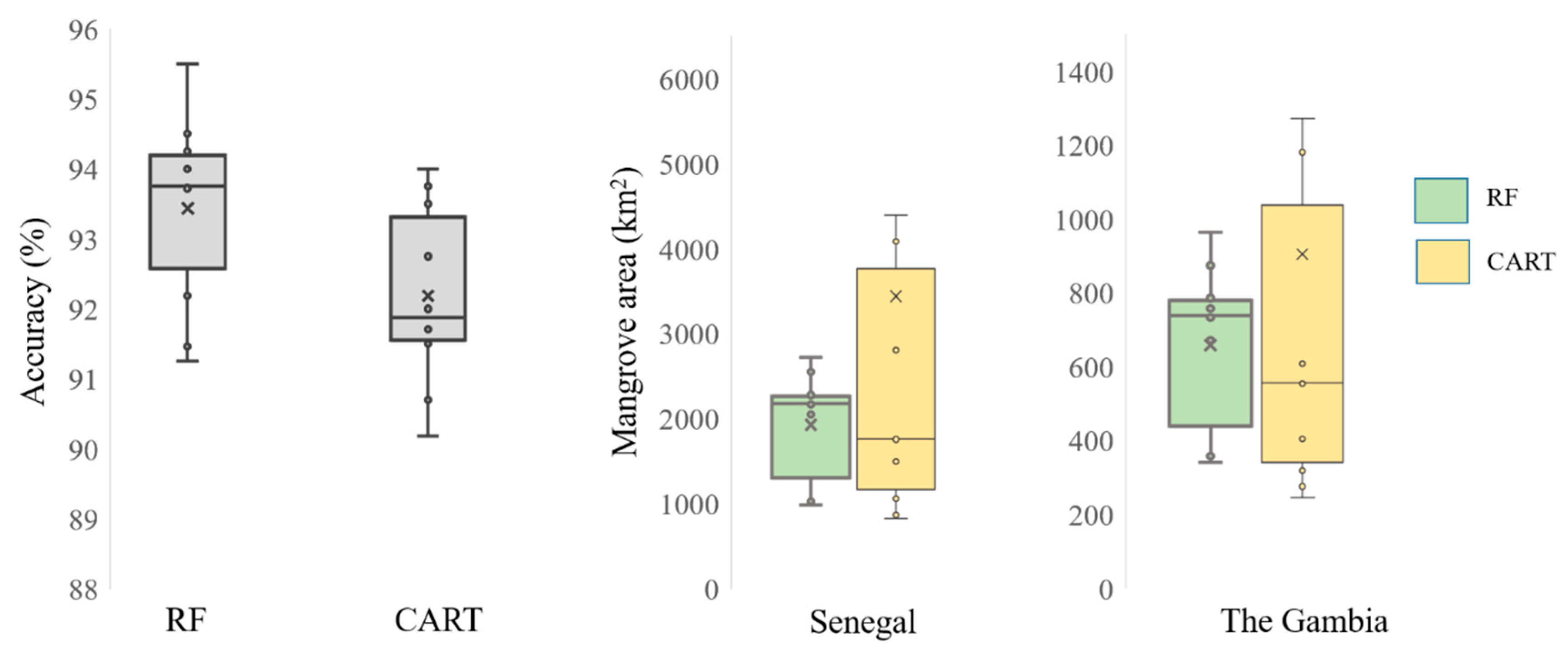
Table 2 lists accuracies per class—both producer’s and user’s accuracy—for the two algorithms used in this study. We report the average accuracy with standard deviations using all 10 iterations for both algorithms (Table 2). The mangrove class has the highest user’s accuracy among the four land cover classes for both algorithms (99.2%–99.56%), closely followed by the ‘other vegetation’ class (95.7%–96.74%). Both classifiers were only moderately successful in distinguishing between water and sandy soil often present along the river (user’s accuracy ranging between 71.49%–75.61% for water and 75.28%–77.53% for sand/soil). The producer’s accuracy follows the same patterns for per class accuracy. The average overall accuracy of the RF-generated classified image is 93.44% (κ = 0.89), while that for the CART-generated image is 92.18% (κ = 0.86) (Figure 4).
3.2. Mangrove Extent in Senegal and The Gambia
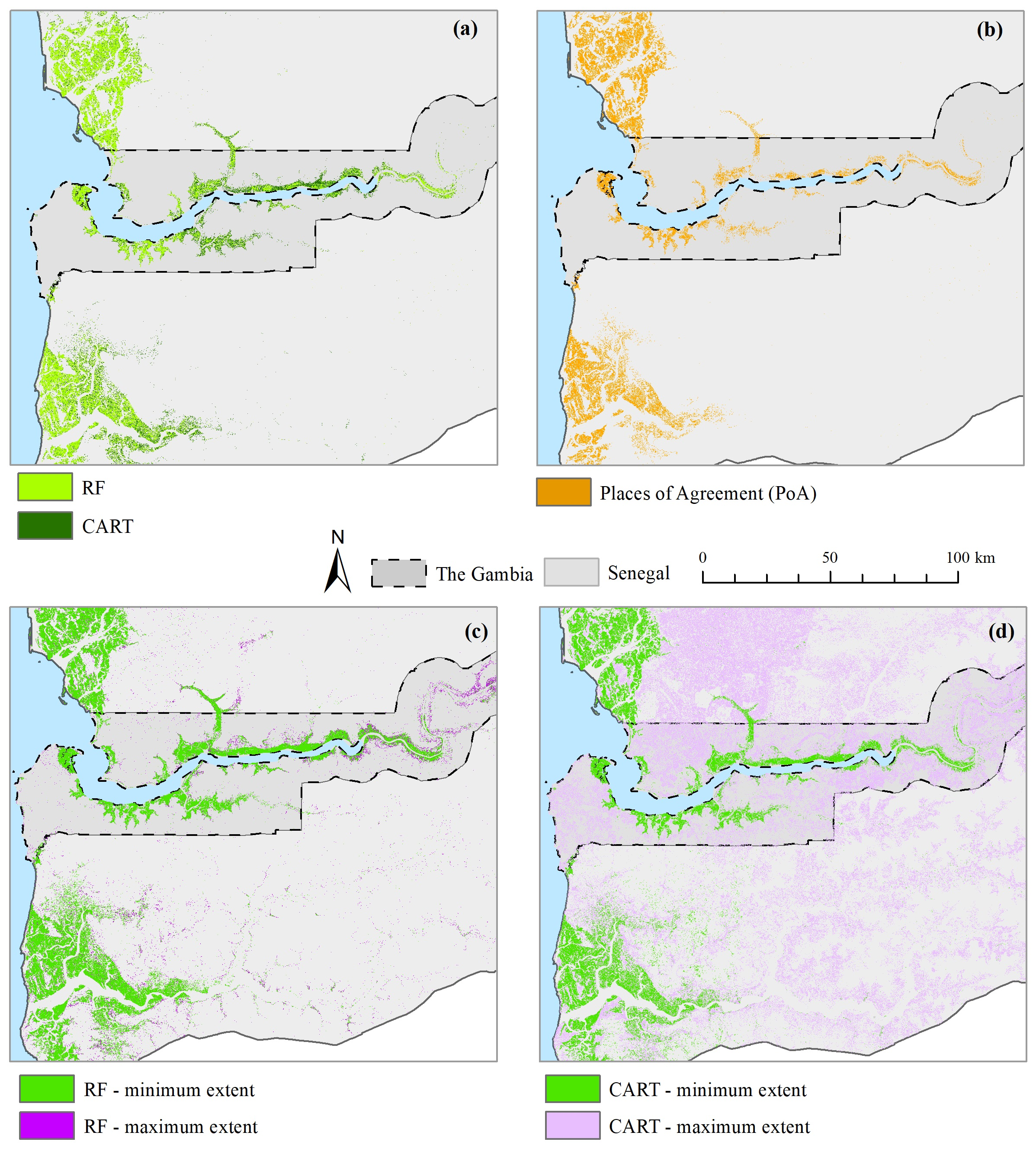
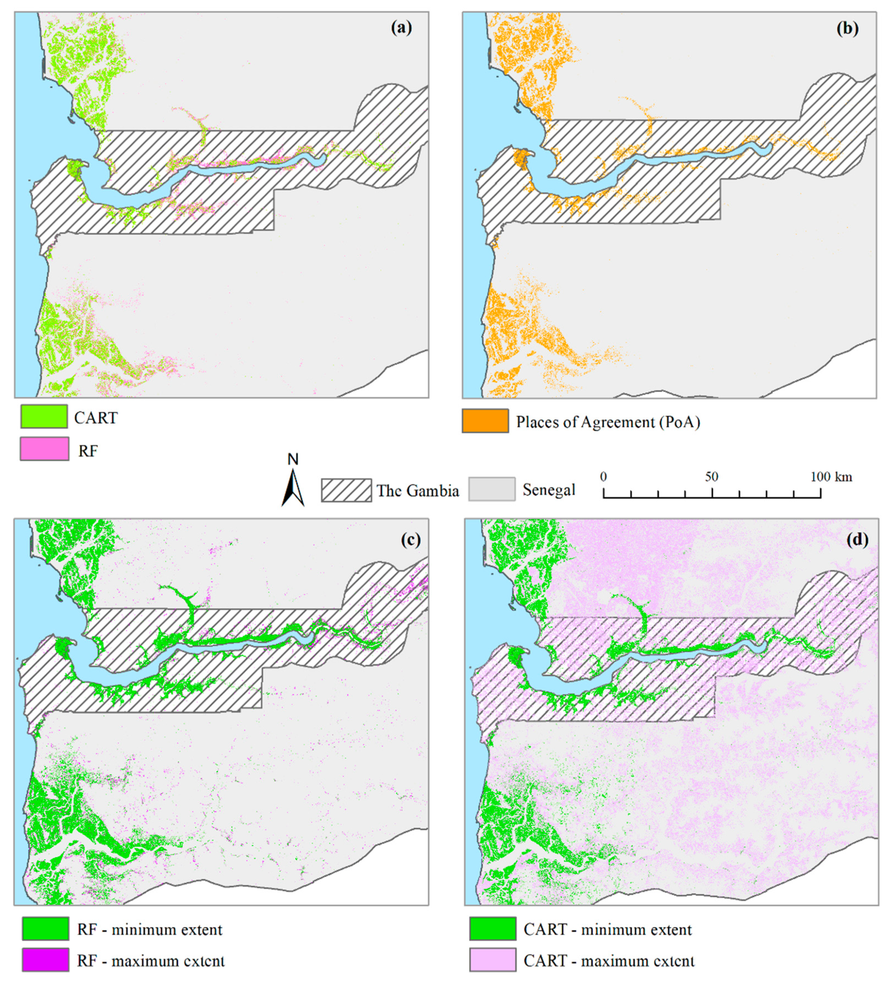
While all 20 iterations for the two classifiers show over 90% overall accuracy, the resulting maps vary widely in terms of mangrove extent (Figure 4). The extent predicted by the CART have a wider range and a lower average compared to those predicted by the RF for both countries (Figure 4). The 10 iterations for the RF and the CART agree on 714.28 km2 and 507.26 km2 of mangroves in Senegal, respectively (Figure 5a). Similarly, the overlapping mangrove areas are 237.14 km2 and 131.05 km2 for The Gambia as per RF and CART, respectively (Figure 5a). Both classifiers agree on approximately 506.59 km2 under mangrove cover in Senegal, whereas the PoA are around 129.64 km2 in The Gambia (Figure 5b).
For Senegal, mangrove extent varies from 990 km2 to 2726 km2 according to the 10 iterations of the RF classifier (Figure 5c), while that for CART vary between 826 km2 to 4396 km2 with an outlier of 15,352 km2 (Figure 5d). For The Gambia, mangrove extent range between 340 km2 to 964 km2 as per RF (Figure 5c), and 245 km2 to 1271 km2 with an outlier of 3630 km2 as per CART (Figure 5d).
4. Discussion
The objective of the current work was to evaluate open data and tools for regular monitoring, especially suitable for in-country technicians who can complete the analysis and share results with the landscape managers and decision-makers who can then make an informed decision. We ran ten iterations for each of the algorithms (total 20) to derive the range of accuracies and mangrove extent generated by these algorithms. In general, this cross-validation indicates agreement among the RF iterations indicating robustness of this classifier. Seven out of ten RF iterations for Senegal predict mangrove extent in the range of 2050–2726 km2, with one iteration predicting less than 1000 km2 (Figure 4). For The Gambia, the RF predictions have a wider range, with three iterations predicting mangrove extent less than 360 km2, five iterations predicting in the range of 670–760 km2, and two iterations predicting over 800 km2 of mangrove cover (Figure 4). The CART iterations predict a wider range of mangrove extent compared to those by RF for both countries. For Senegal, while three iterations predict approximately 1000 km2 of mangroves, three iterations predict in the range of 1500–1800 km2. One CART iteration grossly overestimates mangrove extent (15,352 km2; Figure 5d) even though it had a high overall accuracy (93.5%), likely due to the inherent CART property of wide variability in predicted estimates [91]. This pattern of gross overestimation by at least one CART iteration holds true for The Gambia, while one iteration predicted 3630 km2 of mangrove extent (Figure 5d). Four out of ten iterations predicted ≤400 km2 mangroves in The Gambia, while three iterations predicted mangroves in the range of 550–610 km2. These findings indicate that the same satellite data-classifier combination, based on a discrete classification of Sentinel-2 pixels, can provide a range of estimates for mangrove extent (Figure 4), running into the problem of over- or under-prediction. In this study, this wide range of estimates is an artifact of different sets of training/testing points, which underscores the importance of collecting reference points from ‘pure pixels’ per se, i.e., avoiding mixed environment, such as swampy savannas, or salty bare soils. This lack of consistency across iterations, along with occasional overestimations, also highlights the need for cross-validation in mapping and monitoring natural resources so as to avoid false positives. There are several ways for achieving higher accuracy, including tuning the classifiers by identifying the most accurate parameters, and collecting highly reliable set of training/testing points. However, our findings also highlight the need of examining the outputs more carefully, and not just focusing on the accuracy of the output maps.
One way to avoid false positives would be running multiple iterations of the selected classifier, and then identifying the PoA. In this study, we first quantified PoA for each classifier separately, and then quantified PoA between the two classifiers (Figure 5b). However, for landscape managers, the spatial distribution of PoA might be more meaningful than the overall area. The PoA approach described here can serve as a-priori data set and help the managers by directing their efforts to validating the regions where the iterations did not agree upon. It will be helpful in terms of SDG reporting to include a spatially explicit uncertainty map, with each annual report to highlight regions with high confidence in prediction, but more importantly regions with high uncertainty because of the wide range in model predictions. Another advantage of this PoA approach is its flexibility in terms of input satellite data. While we used Sentinel-2 optical data, Sentinel-1, or radar data from other sources might be better suited for regions with persistent cloud covers, such as tropical countries in Africa or Asia. Decision-makers interested in examining long-term change trajectory might also consider utilizing the entire Landsat record (also available on GEE).
It should be noted that any direct comparison between available datasets using other input data or methods should not be used for tracking national-level progress, or lack thereof. To the best of our knowledge, the most updated mangrove estimates for these countries are from 2016, derived from a 2010 baseline (Table 3) developed under the global mangrove watch (GMW) project [1]. This study used ALOS PALSAR and Landsat data to generate a baseline for 2010, and then used JERS-1, ALOS PALSAR, and ALOS-2 PALSAR-2 to quantify changes between 1996 and 2016 from the 2010 baseline. As per this dataset, mangrove extent in 2016 is 1288.17 km2 and 577.48 km2 in Senegal and The Gambia, respectively. Another recent study [93] provided 2012 mangrove estimates for Senegal and The Gambia (Table 3) among other countries, based on a combined estimation derived from three existing datasets—the global forest gains/losses and fractional cover [94], mangrove forests of the world [38] and terrestrial ecoregions of the world [95]. The primary methodological difference between [93] and other existing data sets (Table 3) is that [93] assigns a sub-pixel percentage value for each mangrove pixel identified by the discrete classification system adopted in other studies, thus reporting only a fraction of mangrove extent compared to other estimates that were based on presence/absence of mangrove pixels.
The authors of [93] pointed out that discrete classification approach is often plagued with overestimation. However, it is challenging, if not almost impossible, to adopt a continuous classification approach for SDG reporting, because such an approach needs a historical comparison where the known accuracy or detailed field data from prior years are often missing. It is also important to consider mangroves as an ecosystem, where mud banks, salty bare soils, and tidal channels are considered integral parts of the ecosystem. However, such detailed mapping often requires prolonged field data collection effort, which might not be a pragmatic recommendation everywhere. The PoA approach presented here relies on input data of a finer spatial scale (20 m) and provides a middle-ground approach between complicated continuous mapping effort and overestimation resulting from discrete classification based on coarser-resolution input data. Even though there are still internet connectivity issues in many countries that might prevent the in-country analysts to generate and/or display maps on GEE, with freely available data, robust methods, and cloud computing platforms, it is easier than ever to conduct regular monitoring for any natural resources. However, our findings indicate that solely reporting estimates, without uncertainty attached to the report, could lead to erroneous decision-making. It is thus our recommendation to consider the spatial distribution of the ecosystem of interest (mangrove forests in this study), and report a confidence map or uncertainty analysis along with the thematic map. Such an approach not only will look beyond the accuracy assessments of thematic maps but can also reduce the necessity for post-classification on-the-ground validation.
5. Conclusions
Landscape managers often need to conduct repeated monitoring of natural resources, such as mangrove forests, on an annual or semi-annual basis. Such monitoring that uses consistent methods is even more important for documenting progress at a national level, e.g., tracking SDG environmental indicators. Satellite data is freely available on cloud computing platforms, along with easily implementable robust methods, such as machine-learning algorithms, including RF and CART, thus offering an unprecedented ease in processing enormous amount of data with no local requirement for advanced computing resources. While many prior studies have used such approaches in quantifying mangroves and other natural resources, our findings indicate that predictions can have a wide range depending on the classifier and the set of training and testing data used. At least one iteration for each of the classifiers used in this study grossly overestimated mangrove extent in Senegal and The Gambia. Hence, such an approach must also include a confidence map to avoid the risk of under- or over-predicting mangrove extent. We acknowledge the potential of utilizing such nearly-automated approaches in decision making over a larger region, but recommend using these with uncertainty analysis, especially in heterogeneous landscapes.
Author Contributions
Conceptualization, P.M. and X.L.; methodology, P.M.; writing—original draft preparation, P.M.; writing—review and editing, X.L., T.E.F., and D.L.; funding acquisition, T.E.F.
Funding
This research was funded by the NASA Carbon Monitoring System Program Project “Estimating Total Ecosystem Carbon in Blue Carbon and Tropical Peatland Ecosystems” (16-CMS16-0073). We furthermore acknowledge funding from the NASA Applied Sciences Program on using Earth Observation in support of the Sustainable Development Goals.
Acknowledgments
We acknowledge constructive feedback from four anonymous reviewers. PM would like to thank colleagues at the University of Delaware for discussion and feedback on an earlier draft.
Conflicts of Interest
The authors declare no conflict of interest.
References
- Bunting, P.; Rosenqvist, A.; Lucas, R.; Rebelo, L.-M.; Hilarides, L.; Thomas, N.; Hardy, A.; Itoh, T.; Shimada, M.; Finlayson, C. The Global Mangrove Watch—A New 2010 Global Baseline of Mangrove Extent. Remote Sens. 2018, 10, 1669. [Google Scholar] [CrossRef] [Green Version]
- Donato, D.C.; Kauffman, J.B.; Murdiyarso, D.; Kurnianto, S.; Stidham, M.; Kanninen, M. Mangroves among the most carbon-rich forests in the tropics. Nat. Geosci. 2011, 4, 293–297. [Google Scholar] [CrossRef]
- Page, S.E.; Rieley, J.O.; Banks, C.J. Global and regional importance of the tropical peatland carbon pool. Glob. Chang. Biol. 2011, 17, 798–818. [Google Scholar] [CrossRef] [Green Version]
- Siikamaki, J.; Sanchirico, J.N.; Jardine, S.L. Global economic potential for reducing carbon dioxide emissions from mangrove loss. Proc. Natl. Acad. Sci. USA 2012, 109, 14369–14374. [Google Scholar] [CrossRef] [PubMed] [Green Version]
- Murdiyarso, D.; Purbopuspito, J.; Kauffman, J.B.; Warren, M.W.; Sasmito, S.D.; Donato, D.C.; Manuri, S.; Krisnawati, H.; Taberima, S.; Kurnianto, S. The potential of Indonesian mangrove forests for global climate change mitigation. Nat. Clim. Chang. 2015, 5, 1089–1092. [Google Scholar] [CrossRef]
- Rovai, A.S.; Twilley, R.R.; Castañeda-Moya, E.; Riul, P.; Cifuentes-Jara, M.; Manrow-Villalobos, M.; Horta, P.A.; Simonassi, J.C.; Fonseca, A.L.; Pagliosa, P.R. Global controls on carbon storage in mangrove soils. Nat. Clim. Chang. 2018, 8, 534–538. [Google Scholar] [CrossRef]
- Hutchison, J.; Manica, A.; Swetnam, R.; Balmford, A.; Spalding, M. Predicting Global Patterns in Mangrove Forest Biomass: Global patterns in mangrove biomass. Conserv. Lett. 2014, 7, 233–240. [Google Scholar] [CrossRef] [Green Version]
- Lee, S.Y.; Primavera, J.H.; Dahdouh-Guebas, F.; McKee, K.; Bosire, J.O.; Cannicci, S.; Diele, K.; Fromard, F.; Koedam, N.; Marchand, C.; et al. Ecological role and services of tropical mangrove ecosystems: A reassessment: Reassessment of mangrove ecosystem services. Glob. Ecol. Biogeogr. 2014, 23, 726–743. [Google Scholar] [CrossRef]
- Gedan, K.B.; Kirwan, M.L.; Wolanski, E.; Barbier, E.B.; Silliman, B.R. The present and future role of coastal wetland vegetation in protecting shorelines: Answering recent challenges to the paradigm. Clim. Chang. 2011, 106, 7–29. [Google Scholar] [CrossRef]
- Giri, C.; Pengra, B.; Zhu, Z.; Singh, A.; Tieszen, L.L. Monitoring mangrove forest dynamics of the Sundarbans in Bangladesh and India using multi-temporal satellite data from 1973 to 2000. Estuar. Coast. Shelf Sci. 2007, 73, 91–100. [Google Scholar] [CrossRef]
- Kuenzer, C.; Tuan, V.Q. Assessing the ecosystem services value of Can Gio Mangrove Biosphere Reserve: Combining earth-observation- and household-survey-based analyses. Appl. Geogr. 2013, 45, 167–184. [Google Scholar] [CrossRef]
- Mondal, P.; Trzaska, S.; de Sherbinin, A. Landsat-Derived Estimates of Mangrove Extents in the Sierra Leone Coastal Landscape Complex during 1990–2016. Sensors 2018, 18, 12. [Google Scholar] [CrossRef] [PubMed] [Green Version]
- Brown, I.; Mwansasu, S.; Westerberg, L.-O. L-Band Polarimetric Target Decomposition of Mangroves of the Rufiji Delta, Tanzania. Remote Sens. 2016, 8, 140. [Google Scholar] [CrossRef] [Green Version]
- Dan, T.T.; Chen, C.F.; Chiang, S.H.; Ogawa, S. Mapping and change analysis in mangrove forest by using Landsat imagery. In Xxiii Isprs Congress, Commission Viii; Halounova, L., Safar, V., Raju, P.L.N., Planka, L., Zdimal, V., Kumar, T.S., Faruque, F.S., Kerr, Y., Ramasamy, S.M., Comiso, J., et al., Eds.; Copernicus Gesellschaft Mbh: Gottingen, Germany, 2016; Volume 3, pp. 109–116. [Google Scholar]
- De Santiago, F.F.; Kovacs, J.M.; Lafrance, P. An object-oriented classification method for mapping mangroves in Guinea, West Africa, using multipolarized ALOS PALSAR L-band data. Int. J. Remote Sens. 2013, 34, 563–586. [Google Scholar] [CrossRef]
- Fatoyinbo, T.E.; Simard, M. Height and biomass of mangroves in Africa from ICESat/GLAS and SRTM. Int. J. Remote Sens. 2013, 34, 668–681. [Google Scholar] [CrossRef]
- Giri, C.; Muhlhausen, J. Mangrove forest distributions and dynamics in Madagascar (1975–2005). Sensors 2008, 8, 2104–2117. [Google Scholar] [CrossRef] [Green Version]
- Hoppe-Speer, S.C.L.; Adams, J.B.; Bailey, D. Present state of mangrove forests along the Eastern Cape coast, South Africa. Wetl. Ecol. Manag. 2015, 23, 371–383. [Google Scholar] [CrossRef]
- Hoppe-Speer, S.C.; Adams, J.B.; Rajkaran, A. Mangrove expansion and population structure at a planted site, East London, South Africa. South. For. A J. For. Sci. 2015, 77, 131–139. [Google Scholar] [CrossRef]
- Kovacs, J.M.; de Santiago, F.F.; Bastien, J.; Lafrance, P. An Assessment of Mangroves in Guinea, West Africa, Using a Field and Remote Sensing Based Approach. Wetlands 2010, 30, 773–782. [Google Scholar] [CrossRef]
- Kuenzer, C.; van Beijma, S.; Gessner, U.; Dech, S. Land surface dynamics and environmental challenges of the Niger Delta, Africa: Remote sensing-based analyses spanning three decades (1986–2013). Appl. Geogr. 2014, 53, 354–368. [Google Scholar] [CrossRef]
- Lagomasino, D.; Fatoyinbo, T.; Lee, S.; Feliciano, E.; Trettin, C.; Shapiro, A.; Mangora, M.M. Measuring mangrove carbon loss and gain in deltas. Environ. Res. Lett. 2019, 14, 025002. [Google Scholar] [CrossRef]
- Macamo, C.C.F.; Massuanganhe, E.; Nicolau, D.K.; Bandeira, S.O.; Adams, J.B. Mangrove’s response to cyclone Eline (2000): What is happening 14 years later. Aquat. Bot. 2016, 134, 10–17. [Google Scholar] [CrossRef]
- Omo-Irabor, O.O.; Olobaniyi, S.B.; Akunna, J.; Venus, V.; Maina, J.M.; Paradzayi, C. Mangrove vulnerability modelling in parts of Western Niger Delta, Nigeria using satellite images, GIS techniques and Spatial Multi-Criteria Analysis (SMCA). Environ. Monit. Assess. 2011, 178, 39–51. [Google Scholar] [CrossRef] [PubMed]
- Otero, V.; Quisthoudt, K.; Koedam, N.; Dahdouh-Guebas, F. Mangroves at Their Limits: Detection and Area Estimation of Mangroves along the Sahara Desert Coast. Remote Sens. 2016, 8, 512. [Google Scholar] [CrossRef] [Green Version]
- Salami, A.T.; Akinyede, J.; de Gier, A. A preliminary assessment of NigeriaSat-1 for sustainable mangrove forest monitoring. Int. J. Appl. Earth Obs. Geoinf. 2010, 12, S18–S22. [Google Scholar] [CrossRef]
- Vasconcelos, M.J.P.; Mussá Biai, J.C.; Araújo, A.; Diniz, M.A. Land cover change in two protected areas of Guinea-Bissau (1956–1998). Appl. Geogr. 2002, 22, 139–156. [Google Scholar] [CrossRef]
- Blasco, F.; Gauquelin, T.; Rasolofoharinoro, M.; Denis, J.; Aizpuru, M.; Caldairou, V. Recent advances in mangrove studies using remote sensing data. Mar. Freshw. Res. 1998, 49, 287–296. [Google Scholar] [CrossRef] [Green Version]
- Giri, C. Observation and Monitoring of Mangrove Forests Using Remote Sensing: Opportunities and Challenges. Remote Sens. 2016, 8, 783. [Google Scholar] [CrossRef] [Green Version]
- Heumann, B.W. Satellite remote sensing of mangrove forests: Recent advances and future opportunities. Prog. Phys. Geogr. 2011, 35, 87–108. [Google Scholar] [CrossRef]
- Almahasheer, H.; Aljowair, A.; Duarte, C.M.; Irigoien, X. Decadal stability of Red Sea mangroves. Estuar. Coast. Shelf Sci. 2016, 169, 164–172. [Google Scholar] [CrossRef] [Green Version]
- Dutta, D.; Das, P.K.; Paul, S.; Sharma, J.R.; Dadhwal, V.K. Assessment of ecological disturbance in the mangrove forest of Sundarbans caused by cyclones using MODIS time-series data (2001–2011). Nat. Hazards 2015, 79, 775–790. [Google Scholar] [CrossRef]
- Dutta, D.; Das, P.K.; Paul, S.; Sharma, J.R.; Dhadwal, V.K. Spatio-temporal assessment of ecological disturbance and its intensity in the mangrove forest using modis derived disturbance index. In ISPRS Technical Commission Viii Symposium; Dadhwal, V.K., Diwakar, P.G., Seshasai, M.V.R., Raju, P.L.N., Hakeem, A., Eds.; Copernicus Gesellschaft Mbh: Gottingen, Germany, 2014; Volume 40, pp. 555–559. [Google Scholar]
- Fatoyinbo, T.E.; Simard, M.; Washington-Allen, R.A.; Shugart, H.H. Landscape-scale extent, height, biomass, and carbon estimation of Mozambique′s mangrove forests with Landsat ETM+ and Shuttle Radar Topography Mission elevation data. J. Geophys. Res. Biogeosci. 2008, 113, G02S06. [Google Scholar] [CrossRef]
- Fromard, F.; Vega, C.; Proisy, C. Half a century of dynamic coastal change affecting mangrove shorelines of French Guiana. A case study based on remote sensing data analyses and field surveys. Mar. Geol. 2004, 208, 265–280. [Google Scholar] [CrossRef]
- Ghosh, M.K.; Kumar, L.; Roy, C. Mapping Long-Term Changes in Mangrove Species Composition and Distribution in the Sundarbans. Forests 2016, 7, 305. [Google Scholar] [CrossRef] [Green Version]
- Giri, C.; Long, J.; Abbas, S.; Murali, R.M.; Qamer, F.M.; Pengra, B.; Thau, D. Distribution and dynamics of mangrove forests of South Asia. J. Environ. Manag. 2015, 148, 101–111. [Google Scholar] [CrossRef]
- Giri, C.; Ochieng, E.; Tieszen, L.L.; Zhu, Z.; Singh, A.; Loveland, T.; Masek, J.; Duke, N. Status and distribution of mangrove forests of the world using earth observation satellite data. Glob. Ecol. Biogeogr. 2011, 20, 154–159. [Google Scholar] [CrossRef]
- Giri, S.; Mukhopadhyay, A.; Hazra, S.; Mukherjee, S.; Roy, D.; Ghosh, S.; Ghosh, T.; Mitra, D. A study on abundance and distribution of mangrove species in Indian Sundarban using remote sensing technique. J. Coast. Conserv. 2014, 18, 359–367. [Google Scholar] [CrossRef]
- Godoy, M.D.P.; de Andrade Meireles, A.J.; de Lacerda, L.D. Mangrove Response to Land Use Change in Estuaries along the Semiarid Coast of Ceará, Brazil. J. Coast. Res. 2018, 34, 524. [Google Scholar] [CrossRef]
- Hamilton, S. Assessing the role of commercial aquaculture in displacing mangrove forest. Bull. Mar. Sci. 2013, 89, 585–601. [Google Scholar] [CrossRef]
- Hirata, Y.; Tabuchi, R.; Patanaponpaiboon, P.; Poungparn, S.; Yoneda, R.; Fujioka, Y. Estimation of aboveground biomass in mangrove forests using high-resolution satellite data. J. For. Res. 2014, 19, 34–41. [Google Scholar] [CrossRef]
- Kamal, M.; Phinn, S.; Johansen, K. Object-Based Approach for Multi-Scale Mangrove Composition Mapping Using Multi-Resolution Image Datasets. Remote Sens. 2015, 7, 4753–4783. [Google Scholar] [CrossRef] [Green Version]
- Kamthonkiat, D.; Rodfai, C.; Saiwanrungkul, A.; Koshimura, S.; Matsuoka, M. Geoinformatics in mangrove monitoring: Damage and recovery after the 2004 Indian Ocean tsunami in Phang Nga, Thailand. Nat. Hazards Earth Syst. Sci. 2011, 11, 1851–1862. [Google Scholar] [CrossRef]
- Kanniah, K.D.; Sheikhi, A.; Cracknell, A.P.; Goh, H.C.; Tan, K.P.; Ho, C.S.; Rasli, F.N. Satellite Images for Monitoring Mangrove Cover Changes in a Fast Growing Economic Region in Southern Peninsular Malaysia. Remote Sens. 2015, 7, 14360–14385. [Google Scholar] [CrossRef] [Green Version]
- Kirui, K.B.; Kairo, J.G.; Bosire, J.; Viergever, K.M.; Rudra, S.; Huxham, M.; Briers, R.A. Mapping of mangrove forest land cover change along the Kenya coastline using Landsat imagery. Ocean Coast. Manag. 2013, 83, 19–24. [Google Scholar] [CrossRef]
- Leimgruber, P.; Kelly, D.S.; Steininger, M.K.; Brunner, J.; Muller, T.; Songer, M. Forest cover change patterns in Myanmar (Burma) 1990–2000. Environ. Conserv. 2005, 32, 356–364. [Google Scholar] [CrossRef] [Green Version]
- LeMarie, M.; van der Zaag, P.; Menting, G.; Bacluete, E.; Schotanus, D. The use of remote sensing for monitoring environmental indicators: The case of the Incomati estuary, Mozambique. Phys. Chem. Earth 2006, 31, 857–863. [Google Scholar] [CrossRef]
- Liu, K.; Liu, L.; Liu, H.X.; Li, X.; Wang, S.G. Exploring the effects of biophysical parameters on the spatial pattern of rare cold damage to mangrove forests. Remote Sens. Environ. 2014, 150, 20–33. [Google Scholar] [CrossRef]
- Manna, S.; Mondal, P.P.; Mukhopadhyay, A.; Akhand, A.; Hazra, S.; Mitra, D. Vegetation cover change analysis from multi-temporal satellite data in Jharkhali Island, Sundarbans, India. Indian J. Geo Mar. Sci. 2013, 42, 331–342. [Google Scholar]
- Misra, A.; Murali, R.M.; Vethamony, P. Assessment of the land use/land cover (LU/LC) and mangrove changes along the Mandovi-Zuari estuarine complex of Goa, India. Arab. J. Geosci. 2015, 8, 267–279. [Google Scholar] [CrossRef]
- Monzon, A.K.; Reyes, S.R.; Veridiano, R.K.; Tumaneng, R.; De Alban, J.D. Synergy of optical and SAR data for mapping and monitoring mangroves. In XXIII ISPRS Congress, Commission VI; Halounova, L., Safar, V., Gong, J., Hanzl, V., Wu, H., Vyas, A., Wang, L., Musikhin, I., Tsai, F., Gruen, A., et al., Eds.; Copernicus Gesellschaft Mbh: Gottingen, Germany, 2016; Volume 41, pp. 259–266. [Google Scholar]
- Reddy, C.S.; Satish, K.V.; Pasha, S.V.; Jha, C.S.; Dadhwal, V.K. Assessment and monitoring of deforestation and land-use changes (1976–2014) in Andaman and Nicobar Islands, India using remote sensing and GIS. Curr. Sci. 2016, 111, 1492–1499. [Google Scholar] [CrossRef]
- Seto, K.C.; Fragkias, M. Mangrove conversion and aquaculture development in Vietnam: A remote sensing-based approach for evaluating the Ramsar Convention on Wetlands. Glob. Environ. Chang. 2007, 17, 486–500. [Google Scholar] [CrossRef]
- Shapiro, A.C.; Trettin, C.C.; Kuchly, H.; Alavinapanah, S.; Bandeira, S. The Mangroves of the Zambezi Delta: Increase in Extent Observed via Satellite from 1994 to 2013. Remote Sens. 2015, 7, 16504–16518. [Google Scholar] [CrossRef] [Green Version]
- Wang, L.; Sousa, W.P.; Gong, P. Integration of object-based and pixel-based classification for mapping mangroves with IKONOS imagery. Int. J. Remote Sens. 2004, 25, 5655–5668. [Google Scholar] [CrossRef]
- Wang, L.; Jia, M.; Yin, D.; Tian, J. A review of remote sensing for mangrove forests: 1956–2018. Remote Sens. Environ. 2019, 231, 111223. [Google Scholar] [CrossRef]
- Abbas, S.; Qamer, F.M.; Hussain, N.; Saleem, R.; Nitin, K.T. National level assessment of mangrove forest cover in Pakistan. In ISPRS Bhopal 2011 Workshop Earth Observation for Terrestrial Ecosystem; Panigrahy, S., Ray, S.S., Huete, A.R., Eds.; Copernicus Gesellschaft Mbh: Gottingen, Germany, 2011; Volume 38, pp. 187–192. [Google Scholar]
- Abdel-Hamid, A.; Dubovyk, O.; Abou El-Magd, I.; Menz, G. Mapping Mangroves Extents on the Red Sea Coastline in Egypt using Polarimetric SAR and High Resolution Optical Remote Sensing Data. Sustainability 2018, 10, 646. [Google Scholar] [CrossRef] [Green Version]
- Cornforth, W.A.; Fatoyinbo, T.E.; Freemantle, T.P.; Pettorelli, N. Advanced Land Observing Satellite Phased Array Type L-Band SAR (ALOS PALSAR) to Inform the Conservation of Mangroves: Sundarbans as a Case Study. Remote Sens. 2013, 5, 224–237. [Google Scholar] [CrossRef] [Green Version]
- Cougo, M.F.; Souza, P.W.M.; Silva, A.Q.; Fernandes, M.E.B.; dos Santos, J.R.; Abreu, M.R.S.; Nascimento, W.R.; Simard, M. Radarsat-2 Backscattering for the Modeling of Biophysical Parameters of Regenerating Mangrove Forests. Remote Sens. 2015, 7, 17097–17112. [Google Scholar] [CrossRef] [Green Version]
- Lagomasino, D.; Fatoyinbo, T.; Lee, S.; Feliciano, E.; Trettin, C.; Simard, M. A Comparison of Mangrove Canopy Height Using Multiple Independent Measurements from Land, Air, and Space. Remote Sens. 2016, 8, 327. [Google Scholar] [CrossRef] [Green Version]
- Thomas, N.; Lucas, R.; Itoh, T.; Simard, M.; Fatoyinbo, L.; Bunting, P.; Rosenqvist, A. An approach to monitoring mangrove extents through time-series comparison of JERS-1 SAR and ALOS PALSAR data. Wetl. Ecol. Manag. 2015, 23, 3–17. [Google Scholar] [CrossRef]
- Thomas, N.; Lucas, R.; Bunting, P.; Hardy, A.; Rosenqvist, A.; Simard, M. Distribution and drivers of global mangrove forest change, 1996–2010. PLoS ONE 2017, 12, e0179302. [Google Scholar] [CrossRef] [Green Version]
- Thomas, N.; Bunting, P.; Lucas, R.; Hardy, A.; Rosenqvist, A.; Fatoyinbo, T. Mapping Mangrove Extent and Change: A Globally Applicable Approach. Remote Sens. 2018, 10, 1466. [Google Scholar] [CrossRef] [Green Version]
- Rahman, M.M.; Lagomasino, D.; Lee, S.; Fatoyinbo, T.; Ahmed, I.; Kanzaki, M. Improved assessment of mangrove forests in Sundarbans East Wildlife Sanctuary using WorldView 2 and TanDEM-X high resolution imagery. Remote Sens. Ecol. Conserv. 2019, 5, 136–149. [Google Scholar] [CrossRef]
- Chen, B.; Xiao, X.; Li, X.; Pan, L.; Doughty, R.; Ma, J.; Dong, J.; Qin, Y.; Zhao, B.; Wu, Z.; et al. A mangrove forest map of China in 2015: Analysis of time series Landsat 7/8 and Sentinel-1A imagery in Google Earth Engine cloud computing platform. ISPRS J. Photogramm. Remote Sens. 2017, 131, 104–120. [Google Scholar] [CrossRef]
- Diniz, C.; Cortinhas, L.; Nerino, G.; Rodrigues, J.; Sadeck, L.; Adami, M.; Souza-Filho, P. Brazilian Mangrove Status: Three Decades of Satellite Data Analysis. Remote Sens. 2019, 11, 808. [Google Scholar] [CrossRef] [Green Version]
- Li, W.; El-Askary, H.; Qurban, M.A.; Li, J.; ManiKandan, K.P.; Piechota, T. Using multi-indices approach to quantify mangrove changes over the Western Arabian Gulf along Saudi Arabia coast. Ecol. Indic. 2019, 102, 734–745. [Google Scholar] [CrossRef]
- Murray, N.J.; Keith, D.A.; Simpson, D.; Wilshire, J.H.; Lucas, R.M. REMAP: An online remote sensing application for land cover classification and monitoring. Methods Ecol. Evol. 2018, 9, 2019–2027. [Google Scholar] [CrossRef] [Green Version]
- Pimple, U.; Simonetti, D.; Sitthi, A.; Pungkul, S.; Leadprathom, K.; Skupek, H.; Som-ard, J.; Gond, V.; Towprayoon, S. Google Earth Engine Based Three Decadal Landsat Imagery Analysis for Mapping of Mangrove Forests and Its Surroundings in the Trat Province of Thailand. J. Comput. Commun. 2018, 06, 247–264. [Google Scholar] [CrossRef] [Green Version]
- Shrestha, S.; Miranda, I.; Kumar, A.; Pardo, M.L.E.; Dahal, S.; Rashid, T.; Remillard, C.; Mishra, D.R. Identifying and forecasting potential biophysical risk areas within a tropical mangrove ecosystem using multi-sensor data. Int. J. Appl. Earth Obs. Geoinf. 2019, 74, 281–294. [Google Scholar] [CrossRef]
- Kendon, E.J.; Stratton, R.A.; Tucker, S.; Marsham, J.H.; Berthou, S.; Rowell, D.P.; Senior, C.A. Enhanced future changes in wet and dry extremes over Africa at convection-permitting scale. Nat. Commun. 2019, 10, 1794. [Google Scholar] [CrossRef] [Green Version]
- Food and Agriculture Organization of the United Nations. Available online: http://www.fao.org/countryprofiles/index/en/ (accessed on 22 July 2019).
- Friedl, M.; Sulla-Menashe, D. MCD12q1 MODIS/Terra+Aqua Land Cover Type Yearly L3 Global 500m SIN Grid V006 [Data Set]. NASA EOSDIS Land Processes DAAC. Available online: https://doi.org/10.5067/MODIS/MCD12Q1.006 (accessed on 20 July 2019).
- Guèye, A.K.; Janicot, S.; Niang, A.; Sawadogo, S.; Sultan, B.; Diongue-Niang, A.; Thiria, S. Weather regimes over Senegal during the summer monsoon season using self-organizing maps and hierarchical ascendant classification. Part II: Interannual time scale. Clim. Dyn. 2012, 39, 2251–2272. [Google Scholar] [CrossRef]
- Diop, E.S. La côte Ouest-Africaine: Du Saloum (Senegal) a la Mellacoree (Rep de Guinee). ′E ditions de l′ORSTOM. ′Etudes et Theses, Institut Français de Recherche Scientifique pour le Développement en Cooperation, Paris, France, 1990. [Google Scholar]
- Tappan, G.G.; Sall, M.; Wood, E.C.; Cushing, M. Ecoregions and land cover trends in Senegal. J. Arid Environ. 2004, 59, 427–462. [Google Scholar] [CrossRef]
- Navarro, J.A.; Algeet, N.; Fernández-Landa, A.; Esteban, J.; Rodríguez-Noriega, P.; Guillén-Climent, M.L. Integration of UAV, Sentinel-1, and Sentinel-2 Data for Mangrove Plantation Aboveground Biomass Monitoring in Senegal. Remote Sens. 2019, 11, 77. [Google Scholar] [CrossRef] [Green Version]
- Simard, M.; Fatoyinbo, L.; Smetanka, C.; Rivera-Monroy, V.H.; Castañeda-Moya, E.; Thomas, N.; Van der Stocken, T. Mangrove canopy height globally related to precipitation, temperature and cyclone frequency. Nat. Geosci. 2019, 12, 40–45. [Google Scholar] [CrossRef]
- SUHET. Sentinel-2 User Handbook. 2015. Available online: https://sentinel.esa.int/documents/247904/685211/Sentinel-2_User_Handbook (accessed on 22 July 2019).
- Holben, B.N. Characteristics of maximum-value composite images from temporal AVHRR data. Int. J. Remote Sens. 1986, 7, 1417–1434. [Google Scholar] [CrossRef]
- Roy, D.P. Investigation of the maximum Normalized Difference Vegetation Index (NDVI) and the maximum surface temperature (Ts) AVHRR compositing procedures for the extraction of NDVI and Ts over forest. Int. J. Remote Sens. 1997, 18, 2383–2401. [Google Scholar] [CrossRef]
- Roy, D.P.; Ju, J.; Kline, K.; Scaramuzza, P.L.; Kovalskyy, V.; Hansen, M.; Loveland, T.R.; Vermote, E.; Zhang, C. Web-enabled Landsat Data (WELD): Landsat ETM+ composited mosaics of the conterminous United States. Remote Sens. Environ. 2010, 114, 35–49. [Google Scholar] [CrossRef]
- Cohen, J. A Coefficient of Agreement for Nominal Scales. Educ. Psychol. Meas. 1960, 20, 37–46. [Google Scholar] [CrossRef]
- World Imagery. Available online: http://goto.arcgisonline.com/maps/World_Imagery (accessed on 15 July 2019).
- Breiman, L. Bagging Predictors. Mach. Learn. 1996, 24, 123–140. [Google Scholar] [CrossRef] [Green Version]
- Breiman, L. Random Forests. Mach. Learn. 2001, 45, 5–32. [Google Scholar] [CrossRef] [Green Version]
- Gislason, P.O.; Benediktsson, J.A.; Sveinsson, J.R. Random Forests for land cover classification. Pattern Recognit. Lett. 2006, 27, 294–300. [Google Scholar] [CrossRef]
- Breiman, L.; Friedman, J.H.; Olshen, R.A.; Stone, C.J. Classification and Regression Trees; Wadsworth & Brooks/Cole Advanced Books & Software: Monterey, CA, USA, 1984; ISBN 978-0-412-04841-8. [Google Scholar]
- Hayes, T.; Usami, S.; Jacobucci, R.; McArdle, J.J. Using Classification and Regression Trees (CART) and random forests to analyze attrition: Results from two simulations. Psychol. Aging 2015, 30, 911–929. [Google Scholar] [CrossRef] [PubMed] [Green Version]
- Malekipirbazari, M.; Aksakalli, V. Risk assessment in social lending via random forests. Expert Syst. Appl. 2015, 42, 4621–4631. [Google Scholar] [CrossRef]
- Hamilton, S.E.; Casey, D. Creation of a high spatio-temporal resolution global database of continuous mangrove forest cover for the 21st century (CGMFC-21): CGMFC-21. Glob. Ecol. Biogeogr. 2016, 25, 729–738. [Google Scholar] [CrossRef]
- Hansen, M.C.; Potapov, P.V.; Moore, R.; Hancher, M.; Turubanova, S.A.; Tyukavina, A.; Thau, D.; Stehman, S.V.; Goetz, S.J.; Loveland, T.R.; et al. High-resolution global maps of 21st-century forest cover change. Science 2013, 342, 850–853. [Google Scholar] [CrossRef] [Green Version]
- Olson, D.M.; Dinerstein, E.; Wikramanayake, E.D.; Burgess, N.D.; Powell, G.V.N.; Underwood, E.C.; D’amico, J.A.; Itoua, I.; Strand, H.E.; Morrison, J.C.; et al. Terrestrial Ecoregions of the World: A New Map of Life on Earth. BioScience 2001, 51, 933. [Google Scholar] [CrossRef]
Figure 1.
Land cover types and remotely sensed surface features in the study area. Data on land cover types were extracted from MODIS land cover type global data product (MCD12Q1.006; spatial resolution: 500 m) following the International Geosphere-Biosphere Programme (IGBP) classification for 2016 using Google Earth Engine (GEE) platform. Inset map shows location of the study area within Africa. Maps were created in ArcGIS 10.5.1.

Figure 2.
Spatial distribution of training and testing points from one of the 10 iterations against the backdrop of very high-resolution satellite data (spatial resolution: 1 m) provided by [86].
Figure 2.
Spatial distribution of training and testing points from one of the 10 iterations against the backdrop of very high-resolution satellite data (spatial resolution: 1 m) provided by [86].

Figure 3.
Methodological framework used in this study. Panels (a) and (b) show internal structures of a random forest (RF) classifier (modified after [92], and classification and regression tree (CART) classifier. Panel (c) shows overall workflow with input data (Sentinel-2 top-of-atmosphere (TOA) reflectance data, along with reference points for model training and testing), Google Earth Engine (GEE) classifiers and output maps, including places of agreement (PoA) map.

Figure 4.
Left panel shows range (n = 10 for each classifier) of overall accuracies for the classified maps generated by the random forest (RF) and the classification and regression trees (CART). Right panel shows range of mangrove estimates generated by RF and CART classifiers for Senegal and The Gambia in 2017.

Figure 5.
Spatial distribution of mangrove forests in Senegal and The Gambia as classified by different iterations of the two classifiers: (a) mangrove extent identified by all iterations in Random Forest (RF) and Classification and Regression Trees (CART) showing places of disagreement; (b) Places of Agreement (PoA) between the two classifiers from a total of 20 iterations; (c) spatial distribution of mangroves from the RF iterations with maximum and minimum extent; (d) spatial distribution of mangroves from the CART iterations with maximum and minimum extent.


Table 1.
Proportion of area under different land cover types in 2016 (in %) as extracted from [75] for Senegal and The Gambia.
Table 1.
Proportion of area under different land cover types in 2016 (in %) as extracted from [75] for Senegal and The Gambia.
| Land Cover Description | Senegal | Gambia |
|---|---|---|
| Deciduous Broadleaf Forests: dominated by deciduous broadleaf trees (canopy > 2 m). Tree cover >60%. | 0.100 | - |
| Mixed Forests: dominated by neither deciduous nor evergreen (40–60% of each) tree type (canopy > 2 m). Tree cover >60%. | 0.003 | - |
| Open Shrublands: dominated by woody perennials (1–2 m height) 10–60% cover. | 0.433 | - |
| Woody Savannas: tree cover 30–60% (canopy >2 m). | 0.004 | - |
| Savannas: tree cover 10–30% (canopy >2 m). | 4.410 | 1.316 |
| Grasslands: dominated by herbaceous annuals (<2 m). | 80.430 | 47.599 |
| Permanent Wetlands: permanently inundated lands with 30–60% water cover and >10% vegetated cover. | 1.023 | 5.792 |
| Croplands: at least 60% of area is cultivated cropland. | 11.999 | 42.788 |
| Urban and Built-up Lands: at least 30% impervious surface area including building materials, asphalt and vehicles. | 0.294 | 0.872 |
| Cropland/Natural Vegetation Mosaics: mosaics of small-scale cultivation 40–60% with natural tree, shrub, or herbaceous vegetation. | 0.078 | 0.082 |
| Barren: at least 60% of area is non-vegetated barren (sand, rock, soil) areas with less than 10% vegetation. | 0.390 | 0.245 |
| Water Bodies: at least 60% of area is covered by permanent water bodies. | 0.838 | 1.307 |
Table 2.
The range of per class, overall, producer’s and user’s accuracy for the classifications generated by random forest (RF) and classification and regression trees (CART).
Table 2.
The range of per class, overall, producer’s and user’s accuracy for the classifications generated by random forest (RF) and classification and regression trees (CART).
| Random Forest (RF) | ||||
| Mangrove | Water | Other Vegetation | Sand/Soil | |
| Producer’s accuracy | 99.2% ± 0.71% | 76.65% ± 8% | 99.4% ± 0.97% | 75.2% ± 6.2% |
| User’s accuracy | 99.56% ± 0.51% | 75.61% ± 5.05% | 96.74% ± 2.47% | 77.53% ± 5.62% |
| Overall | 93.44% ± 1.37% | |||
| κ | 0.89 ± 0.02 | |||
| Classification and Regression Trees (CART) | ||||
| Mangrove | Water | Other Vegetation | Sand/Soil | |
| Producer’s accuracy | 98.48% ± 0.92% | 76.9% ± 5.85% | 97.39% ± 2.85% | 70.6% ± 4.99% |
| User’s accuracy | 99.2% ± 0.62% | 71.49% ± 5.74% | 95.7% ± 1.7% | 75.28% ± 5.37% |
| Overall | 92.18% ± 1.29% | |||
| κ | 0.86 ± 0.02 | |||
Table 3.
Comparison of mangrove extent estimates for Senegal and The Gambia derived from existing data sets and work presented here. The estimates from the existing data sets is an approximation and were extracted from the original data sets using ArcMap 10.5.1.
Table 3.
Comparison of mangrove extent estimates for Senegal and The Gambia derived from existing data sets and work presented here. The estimates from the existing data sets is an approximation and were extracted from the original data sets using ArcMap 10.5.1.
| Data Source | Year of Estimate | Spatial Resolution | Area (km2)—Senegal | Area (km2)—The Gambia |
|---|---|---|---|---|
| Mangrove Forests of the World (MFW) [36] | 1997–2000 | 30 m | 1423.10 | 652.37 |
| Global Mangrove Watch (GMW) [6] | 2010 | 25 m | 1325.52 | 587.08 |
| Global Database of Continuous mangrove Forest Cover for the 21st Century (CGMFC-21) [83] | 2012 | 30 m | 155.34 | 48.05 |
| This study–PoA approach | 2017 | 20 m | 506.59 | 129.64 |
© 2019 by the authors. Licensee MDPI, Basel, Switzerland. This article is an open access article distributed under the terms and conditions of the Creative Commons Attribution (CC BY) license (http://creativecommons.org/licenses/by/4.0/).
Share and Cite
MDPI and ACS Style
Mondal, P.; Liu, X.; Fatoyinbo, T.E.; Lagomasino, D. Evaluating Combinations of Sentinel-2 Data and Machine-Learning Algorithms for Mangrove Mapping in West Africa. Remote Sens. 2019, 11, 2928. https://doi.org/10.3390/rs11242928
AMA Style
Mondal P, Liu X, Fatoyinbo TE, Lagomasino D. Evaluating Combinations of Sentinel-2 Data and Machine-Learning Algorithms for Mangrove Mapping in West Africa. Remote Sensing. 2019; 11(24):2928. https://doi.org/10.3390/rs11242928
Chicago/Turabian StyleMondal, Pinki, Xue Liu, Temilola E. Fatoyinbo, and David Lagomasino. 2019. "Evaluating Combinations of Sentinel-2 Data and Machine-Learning Algorithms for Mangrove Mapping in West Africa" Remote Sensing 11, no. 24: 2928. https://doi.org/10.3390/rs11242928
Note that from the first issue of 2016, this journal uses article numbers instead of page numbers. See further details here.