Evaluation of UAV LiDAR for Mapping Coastal Environments
by
 , , , , ,
Yi-Chun Lin
1 ,
,
Yi-Ting Cheng
1,
Tian Zhou
1,
Radhika Ravi
1,
Seyyed Meghdad Hasheminasab
1,
John Evan Flatt
1,
Cary Troy
1 and 
Ayman Habib
1,2,* 1
Lyles School of Civil Engineering, Purdue University, West Lafayette, IN 47907, USA
2
Civil Engineering Center for Applications of UAS for a Sustainable Environment (CE-CAUSE), Lyles School of Civil Engineering, Purdue University, West Lafayette, IN 47907, USA
*
Author to whom correspondence should be addressed.
Remote Sens. 2019, 11(24), 2893; https://doi.org/10.3390/rs11242893
Submission received: 8 November 2019
/
Revised: 1 December 2019
/
Accepted: 2 December 2019
/
Published: 4 December 2019
Abstract
:Unmanned Aerial Vehicle (UAV)-based remote sensing techniques have demonstrated great potential for monitoring rapid shoreline changes. With image-based approaches utilizing Structure from Motion (SfM), high-resolution Digital Surface Models (DSM), and orthophotos can be generated efficiently using UAV imagery. However, image-based mapping yields relatively poor results in low textured areas as compared to those from LiDAR. This study demonstrates the applicability of UAV LiDAR for mapping coastal environments. A custom-built UAV-based mobile mapping system is used to simultaneously collect LiDAR and imagery data. The quality of LiDAR, as well as image-based point clouds, are investigated and compared over different geomorphic environments in terms of their point density, relative and absolute accuracy, and area coverage. The results suggest that both UAV LiDAR and image-based techniques provide high-resolution and high-quality topographic data, and the point clouds generated by both techniques are compatible within a 5 to 10 cm range. UAV LiDAR has a clear advantage in terms of large and uniform ground coverage over different geomorphic environments, higher point density, and ability to penetrate through vegetation to capture points below the canopy. Furthermore, UAV LiDAR-based data acquisitions are assessed for their applicability in monitoring shoreline changes over two actively eroding sandy beaches along southern Lake Michigan, Dune Acres, and Beverly Shores, through repeated field surveys. The results indicate a considerable volume loss and ridge point retreat over an extended period of one year (May 2018 to May 2019) as well as a short storm-induced period of one month (November 2018 to December 2018). The foredune ridge recession ranges from 0 m to 9 m. The average volume loss at Dune Acres is 18.2 cubic meters per meter and 12.2 cubic meters per meter within the one-year period and storm-induced period, respectively, highlighting the importance of episodic events in coastline changes. The average volume loss at Beverly Shores is 2.8 cubic meters per meter and 2.6 cubic meters per meter within the survey period and storm-induced period, respectively.
1. Introduction
Coastal erosion can cause significant damages to buildings, infrastructure, utilities, and ecosystems, and mitigating its effect has become increasingly important, especially considering recent climate change manifestations. A well-developed understanding of complex shoreline movement, i.e., their spatial distribution at local, regional, and national scale, as well as their temporal distribution at event-, seasonal-, and decadal-scale, serves as the foundation for effective coastal management. To meet the increasing demand for accurate and recurrent monitoring of coastal change, remote sensing techniques are showing superior performance compared to the conventional time and labor-intensive field survey. A wide range of remote sensing techniques have been used to monitor coastal changes, including satellite imagery, aerial photography, Synthetic Aperture Radar (SAR), ground-penetrating radar, airborne and terrestrial LiDAR, and most recently, Unmanned Aerial Vehicles (UAV) imagery. In particular, terrestrial LiDAR and UAV photogrammetry can rapidly acquire topographic data with a spatial and temporal resolution that was previously unachievable, which has led to significant advances in understanding complex erosion processes [1,2,3,4]. While UAV surveys have a clear advantage in terms of low-cost equipment, rapid survey time, and ease of deployment, terrestrial LiDAR has been proven to produce more reliable surface representation in complex geomorphic environments [2,4].
In this paper, we describe the development, evaluation, and application of a UAV-based mobile mapping system equipped with high-resolution topographic LiDAR, Red-Green-Blue (RGB) imaging system, and an integrated Global Navigation Satellite System/Inertial Navigation System (GNSS/INS). The system went through a rigorous system calibration, which is crucial for direct georeferencing, reconstructing accurate LiDAR point clouds, and integrating 3D point clouds with 2D imagery. Field surveys were conducted on Dana Island, Turkey, and along the Indiana beaches of southern Lake Michigan, USA. The former contains a range of topographies and vegetation types, while the latter is an actively eroding beach. This study first demonstrates the ability of UAV LiDAR for mapping coastal environments by evaluating the quality of UAV LiDAR point clouds and comparing it with UAV image-based point clouds using the Dana Island datasets. The capability of UAV LiDAR for quantifying rapid coastal changes at seasonal- and event-scale is further investigated using the Lake Michigan datasets. This paper starts with a review of the remote sensing techniques used for coastal monitoring. We then describe the UAV-based mobile mapping system, along with an introduction of the study sites and field surveys. Further, we discuss the methodology adopted for assessing the quality of UAV LiDAR point clouds, followed by comparison against UAV photogrammetry, and quantitative estimation of shoreline change. Finally, we present the conclusions of this study and recommendations for future work.
2. Related Work
Remote sensing has been the dominant source of geospatial information for detecting and monitoring coastline changes over time, of which the most common techniques include satellite imagery, aerial photography, airborne LiDAR, terrestrial LiDAR, and UAV photogrammetry. These techniques can be categorized into those which provide 2D planimetric data (i.e., ortho-rectified imagery), and those which reconstruct 3D topographic data (i.e., LiDAR and photogrammetric point clouds). Table 1 summarizes these techniques while listing their merits and shortcomings, as well as reporting their spatial resolution and accuracy. This section reviews the remote sensing techniques that have been used for mapping coastal environments. The discussion begins with satellite imagery and aerial photography, followed by LiDAR technology and photogrammetry, and ultimately, emphasizes the recent development of ground-based and UAV-based LiDAR and photogrammetry.
Ortho-rectified satellite imagery and aerial photography provide planimetric data, which uses a 2D simplification to represent a 3D erosion process. Most data providers deliver georeferenced and rectified images that are ready for end-users to perform spatial analyses. Such datasets typically have large spatial coverage and relatively long time-lapse, and therefore are ideal for regional, long-term analyses. Deis et al. [5] used aerial images of northern Barataria Bay, Louisiana, from 1998 to 2013 to determine marsh shoreline retreat during the period between Hurricane Katrina and the Deepwater Horizon oil spill. Eulie et al. [6] used heads-up-digitized aerial photos to quantify sediment accumulation and shoreline change over one decade (1998–2007) in the Tar-Pamlico estuary, North Carolina. In addition to planimetric positional information, satellite images and aerial photos also provide multispectral or hyperspectral data, which allows users to further identify or classify ground features. Rangel-Buitrago et al. [7] incorporated multiple sources of satellite images and aerial photos to quantify coastal erosion along the Caribbean coast of Colombia. In their research, the water line, which serves as an indicator of the shoreline position, was differentiated and digitized using the infrared band of each image. Despite being the most common data source for shoreline monitoring, imagery data suffers from lack of vertical information and has a relatively coarse spatial resolution; thus resulting in a crude and potentially inaccurate indication of the erosion process that restricts its applications at a local scale.
LiDAR technology is an active remote sensing technique capable of mapping 3D topography of the landscape. Point clouds captured by laser scanners provide a detailed description of the terrain. However, due to its uneven distribution, a re-gridding and interpolation process is usually carried out to generate a Digital Surface Model (DSM). The information loss resulting from such rasterization has a major impact on the achieved accuracy of DSM [8,9]. Over the years, airborne LiDAR data has been a standard topographic product for coastal mapping and has been widely used by the community of geoscientists. Obu et al. [10] used airborne LiDAR datasets captured repetitively over a period of one year to study coastal erosion and volumetric change, together with the accompanying geomorphic process. Tamura et al. [11] integrated topographic data obtained by airborne LiDAR and Real-Time Kinematic Global Navigation Satellite Systems (RTK-GNSS) survey along with stratigraphy data collected by ground-penetrating radar to conduct a high-precision morphostratigraphic analysis of beach ridge evolution. Other studies integrated LiDAR-based DSM with satellite images or aerial photos. The elevation information from DSM facilitated the extraction of urban features (like buildings) and thus, improved the accuracy of coastal mapping [12,13]. In addition to 3D topography, airborne LiDAR is also currently the best technique to obtain bathymetric data, which is crucial to coastal science but challenging to acquire through conventional terrestrial field surveys or boat-based acoustic hydrographic surveys. Launeau et al. [14] used full-waveform LiDAR data to map the bathymetry of the sea bottom in moderately turbid bays. In the United States, the Army Corps of Engineers (USACE) utilizes Coastal Zone Mapping and Imaging LiDAR System (CZMIL) to map coastal zone bathymetry, topography, and other properties [15,16]. The U.S. Geological Survey (USGS) has taken advantage of these new techniques to conduct shoreline change assessment with success [17,18,19]. Current studies concluded that the most restricting factor of LiDAR bathymetry is water clarity [14,16] and thus, it is important to conduct the flight during tidal and current conditions that minimize the water turbidity. Considering weather conditions, as well as budget restrictions, manned aircraft-based coastal surveys cannot be carried out frequently, thus preventing the quantification of coastal response to individual storms and rapid water level fluctuations. As the technology evolves, satellite-borne LiDAR is now a new option for mapping underwater bathymetry. In September 2018, NASA’s Ice, Cloud, and Land Elevation Satellite-2 (ICESat-2) was launched. The instrument carried on the satellite—Advanced Topographic Laser Altimeter System (ATLAS)—shows the potential to map bathymetry. Early on-orbit validation of ICESat-2 bathymetry and quantification of the bathymetric mapping performance can be found in Parrish et al. [20].
Increasing deployment of terrestrial LiDAR for coastal erosion monitoring has been seen in the past decade. Terrestrial LiDAR offers a significant improvement in the spatial resolution and accuracy of topographic data over airborne platforms. Smith et al. [21] presented measurements of blowout topography obtained with annual terrestrial LiDAR surveys carried out over a three-year period. With a 10 mm total propagated positional error, they were able to measure rim displacements smaller than 1 meter. Attributed to the nature of laser scanning, LiDAR has the ability to penetrate vegetation and report elevation below the canopy. Several studies suggested that terrestrial LiDAR provides a suitable representation of the ground surface in vegetated coastal dunes [21,22]. Although the spatial resolution of terrestrial LiDAR data is much higher than airborne data, the point density decreases considerably as the scanner-to-object distance increases. Obtaining a dense point cloud over the entire area of interest often requires multiple stations for the terrestrial LiDAR to be placed for scanning. A registration process is required to align the individual scans to a common mapping frame, which involves surveying several Ground Control Points (GCPs) or manually selecting tie points from overlapping point clouds. Considering the increased time of field survey and data processing, terrestrial LiDAR surveys are typically focused on a specific area of concern as wider-scale analyses are not practical.
Photogrammetry is another well-established technique for 3D topographic mapping. The recent developments in photogrammetric mapping and computer vision led to the emergence of Structure from Motion (SfM). SfM allows fine-resolution 3D reconstruction using overlapping images from consumer-grade cameras, and thus opens the gate to an affordable image-based 3D topographic mapping. UAV imagery is of particular interest for its low-cost, maneuverability, and efficient field surveys. A wide range of commercial and open-source tools (e.g., Pix4D, PhotoScan, DroneDeploy, OpenDroneMap, Regard3D, Meshroom, and COLMAP) enable end-users, without requiring a high level of expertise, to generate high-resolution, high-quality DSMs and orthophotos. These advantages have stimulated a wide range of geoscientists to use image-based techniques as a key tool in generating 3D models [1]. With the help of several GCPs, DSMs and orthophotos generated from UAV imagery can be geo-referenced to a global mapping frame. This workflow has been adopted by several studies for quantifying shoreline movement [23,24,25,26,27]. Moreover, UAV photogrammetry produces both 3D DSMs and 2D orthophotos, which can be easily integrated with other 3D or 2D topographic data. For instance, Mateos et al. [28] combined aerial imagery, UAV imagery, and Persistent Scatterer Interferometric Synthetic Aperture Radar (PSInSAR) for monitoring coastal landslide. Nahon et al. [29] operated a UAV and a terrestrial mobile laser scanning vehicle simultaneously, and used UAV images to observe an optical target, which serves as a kinematic ground control point on the vehicle. By doing this, the number of GCPs can be reduced and it is possible to carry out a single pass survey.
Several studies have compared close-range photogrammetry and UAV-based SfM products with LiDAR, RTK-GNSS, and total station surveys [2,3,4,30,31,32]. Compared to terrestrial LiDAR, UAV surveys have a clear advantage in terms of low-cost equipment, rapid survey time, ease of deployment, and fewer limitations for field survey [2,30]. The resolution and accuracy of SfM are comparable to terrestrial LiDAR in general, and both techniques exhibit a good degree of agreement with GNSS ground truths [2,3]. However, UAV photogrammetry is more sensitive to environmental conditions due to the difficulty in reconstructing 3D surfaces using image-based methods in areas with low texture. Studies have pointed out the lack of quality assessment for UAV photogrammetry in different geomorphic environments [2,3]. Guisado-Pintado et al. [4] assessed the applicability, limitations, and effectiveness of terrestrial LiDAR and UAV SfM techniques when used over a complex beach-dune system. Their results showed that in complex vegetated areas, differences among terrestrial LiDAR and UAV SfM derived surfaces can vary considerably, indicating that both environmental and technical factors are responsible. Studies utilizing wheel-based or UAV-based mobile LiDAR are relatively rare. Elsner et al. [31] compared UAV SfM with wheel-based mobile LiDAR and airborne LiDAR over six different surface types. Their results suggested that UAV point clouds were consistently higher than those obtained by mobile LiDAR and airborne LiDAR. A consistent vertical offset of 6 to 9 cm was observed and the variation of elevation differences was observed to be related to surface properties. Similar findings were reported in Shaw et al. [32], where UAV photogrammetry was compared against UAV LiDAR. The results showed that image-based surfaces had a significant positive bias of 4 to 9 cm when compared to the GNSS ground truth, while LiDAR surfaces were consistent with the ground truth. To conclude, LiDAR provides more realistic surface models in general. The surface models derived from UAV SfM are often of poorer quality when dealing with flat, sandy, and low textured surfaces.
With recent developments in UAV and LiDAR technologies and the reduction of the expense in integrating these technologies, UAV LiDAR has been increasingly used for applications including forestry, archaeology, and infrastructure monitoring [36,37,38,39,40]. Sankey et al. [36] showed that UAV LiDAR is capable of mapping the top of vegetation as well as the bare-earth ground surface. Sankey et al. also proved the reliability of UAV LiDAR by showing that DSMs generated from UAV LiDAR are comparable with those from terrestrial LiDAR. In this study, we present UAV LiDAR for monitoring coastline changes. The strength of UAV LiDAR is demonstrated by comparing the quality of LiDAR point clouds against point clouds generated by image-based techniques. Shoreline change over an actively eroding beach is investigated through repeated surveys within a one-year period.
3. UAV-Based Mobile Mapping System Integration and System Calibration
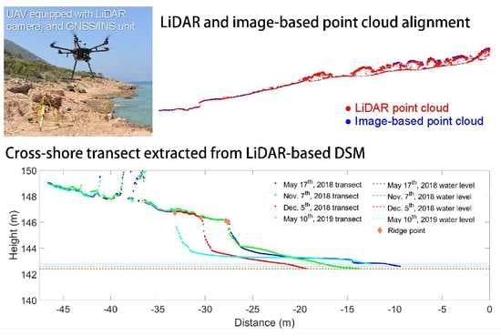
A custom-built UAV-based mobile mapping system is used in this study for simultaneously collecting both LiDAR and imagery data. The system consists of a DJI M600 Pro hexacopter, which carries a laser scanner (Velodyne VLP-32C), a camera (Sony Alpha ILCE-7R), and an integrated GNSS/INS unit (APX-15 UAV V2) for direct georeferencing, as shown in Figure 1. The Velodyne VLP-32C consists of 32 radially oriented laser rangefinders that are aligned vertically from +15˚ to −25˚, thus resulting in a total vertical field of view (FOV) of 40˚. Additionally, the whole laser unit rotates internally to achieve a 360˚ horizontal FOV. The minimum vertical angular resolution is 0.33˚ and the horizontal angular resolution ranges from 0.1˚ to 0.4˚. The point capture rate in a single return mode is around 600,000 points per second. The range accuracy is typically ±3 cm, with a maximum measurement range of 200 m [41]. A Raspberry Pi single-board computer is used to store the LiDAR data in the form of *.pcap files. The Sony Alpha ILCE-7R camera is a 36.4 MP off-the-shelf camera with an image size of 7360 x 4912 pixels. The pixel size is 4.86 μm and the nominal focal length is 35 mm. An Arduino Micro microcontroller board is used to trigger the camera via the Sony multiport at a frame period of 1.5 seconds. Each image event is recorded in the GNSS/INS trajectory via the Alpha 7R hot shoe. For the APX-15 unit, the post-processing positional accuracy is 2 to 5 cm and the accuracy for the roll/pitch and heading is 0.025˚ and 0.08˚, respectively.
System calibration includes the individual sensor calibration and the estimation of the relative position and orientation between each sensor. In this study, the internal characteristics, i.e., the interior orientation parameters (IOPs), of the camera are estimated through a camera calibration procedure similar to the one proposed by He and Habib [42]. The USGS Simultaneous Multi-frame Analytical Calibration (SMAC) distortion model is adopted, which determines the principal distance c, principal point coordinates (xp, yp), and radial and de-centering lens distortion coefficients (K1, K2, P1, P2). The relative position and orientation parameters (hereafter, denoted as mounting parameters) between the onboard sensors (LiDAR and camera) and the GNSS/INS unit are determined through a rigorous system calibration [43,44]. The system calibration simultaneously estimates the mounting parameters by minimizing the discrepancies among conjugate points, linear features, and planar features obtained from LiDAR point clouds and images from different flight lines. The standard deviations of the estimated lever arm components from the system calibration are ±0.9 cm and ±0.6 cm along the x and y directions, respectively, and those of boresight angles are 0.008˚, 0.013˚, and 0.014˚ for roll, pitch, and heading, respectively. The lever arm component along the z direction was determined based on manual measurement and fixed during the system calibration as it would only result in a vertical shift of the point cloud as a whole [43]. Once the mounting parameters are estimated accurately, the captured images and derived LiDAR points by each of the sensors can be directly georeferenced to a common reference frame. More specifically, using the estimated mounting parameters, together with the GNSS/INS trajectory, one can i) reconstruct a georeferenced LiDAR point cloud, and ii) obtain the position and orientation of the camera in a global mapping frame whenever an image is captured. Consequently, both LiDAR point clouds and images are georeferenced to a common reference frame (the UTM coordinate system with the WGS84 as the datum is adopted in this study). It is worth mentioning that no ground control is required in this process.
4. Study Sites and Data Acquisition
Field surveys for this study were carried out on Dana Island, Turkey, and along the Indiana beaches of southern Lake Michigan, USA. The former contains a range of topographies and vegetation types, and thus is selected for assessing the quality of UAV LiDAR point clouds and evaluating the difference between UAV LiDAR and UAV photogrammetry. The latter is an actively eroding beach where we investigate the ability of UAV LiDAR for quantifying rapid coastal changes over one year.
4.1. Dana Island, Turkey
Dana Island is an archaeological site that lies parallel to the south coast of Turkey at 36°11′N33°46′E. The shape of the island is roughly rectangular with dimensions of 2.7 km x 0.8 km. The maximum elevation is 250 m above sea level. The island is covered by limestone and vegetation. Recent research revealed a lower settlement along the northwestern shore and an upper settlement associated with a fortress on the south summit [45]. These settlements can be traced back to the Early Roman period. Ruins of structures with simple rectangular plans and a large number of bell-shaped cisterns are found along the coastline. The field surveys were conducted over the west coast of the island, which is covered by limestone, backed by a densely vegetated hill with an average slope of 20% (as shown in Figure 2).
A total of 1.7 km of coastline was surveyed by five flight missions conducted on July 26th, 27th, 28th, and 29th in 2019. Figure 2 illustrates the surveyed area of each flight mission. In each mission, the UAV-based mobile mapping system collected LiDAR measurements, RGB imagery, and GNSS/INS trajectory. Due to the lack of first-person view, obstacle avoidance concerns, and steep terrain causing difficulties in depth perception, some areas were flown manually to ensure the safety of the aircraft. The mission planning software DJI GS Pro was used for the autonomous flight path programming. Table 2 summarizes the flight configurations of the five flight missions.
4.2. Indiana Shoreline of Southern Lake Michigan, USA
The Great Lakes are experiencing high water levels after a 15-year period of low water levels. With the persistently high water level, storms have much more potential to erode shorelines. Communities have reported erosion that threatens beaches, buildings, and coastal infrastructures. The field surveys took place at two sandy beaches along the Indiana shoreline of Lake Michigan, USA. Both the beaches are small, private residential communities located in the towns of Dune Acres and Beverly Shores. Figure 3 shows the locations and the survey area within the two sites. The length of the beach surveyed is 450 m and 340 m for Dune Acres and Beverly Shores, respectively. Calumet Harbor water level gauge data provided by NOAA (station ID 9087044) [46] was used in this study for determining the water level at the time of the UAV surveys. This is the nearest station to the study sites, and its location is also shown in Figure 3.
A total of seven shoreline surveys were conducted with the UAV-based mobile mapping system. Dune Acres was surveyed on 17 May 2018, 7 November 2018, 5 December 2018, and 10 May 2019. Beverly Shores was surveyed on 19 November 2018, 5 December 2018, and 10 May 2019. Between the November and December surveys, two storms struck the Indiana coastline. Hence, our analysis and discussion focus on the ability of UAV LiDAR for quantifying the annual coastal change, as well as the coastal response to individual storms.
At Dune Acres, the UAV survey covered an extent of approximately 270 m coastline in the 17 May 2018 survey, and approximately 450 m coastline in the 7 November 2018, 5 December 2018, and 10 May 2019 surveys. For Beverly Shores, all the surveys covered approximately 340 m of coastline. The flying altitudes above ground were 10 m to 20 m for Dune Acres and 30 m for Beverly Shores. Flight time was approximately 15 minutes per mission. The system was mostly flown autonomously but was flown manually over areas with nearby obstacles (trees, power lines, etc.). The mission planning software DJI GS Pro was used for the autonomous flight path programming.
5. Methodology
In this section, we present our LiDAR and image-based 3D point cloud reconstruction approaches. We then present the strategies for LiDAR point cloud quality assessment and the qualitative and quantitative comparisons between LiDAR and image-based point clouds. Finally, we describe the strategies for DSM and orthophoto generation and present the metrics for shoreline change quantification.
5.1. LiDAR Point Cloud Reconstruction
Raw LiDAR data includes intensity and range measurements along the direction where the laser beams are pointing to. With the help of the GNSS/INS trajectory, point cloud reconstruction brings all the LiDAR range measurements into one reference frame. By coupling the range and orientation of the laser beams, we can obtain the position of the laser beam footprint relative to the laser unit frame, . The GNSS/INS integration establishes the position, , and orientation, , of the vehicle frame relative to the mapping frame. The laser unit frame and vehicle frame are related using the mounting parameters, which consist of the lever arm, , and the boresight matrix, . Since the laser and the GNSS/INS units are rigidly fixed with respect to each other, the mounting parameters would be time-independent. The 3D coordinates of a ground point, I, in the mapping frame can then be derived as per Equation (1).
The UAV-based mobile mapping system is built in such a way that the rotation axis of the Velodyne laser scanner is approximately parallel to the flying direction, which can be seen in Figure 1b. To exclude points with large sensor-to-object distances, which are assumed to have a lower precision (as will be discussed later), and only focus on the object space, i.e., area below the UAV, we reconstruct a point only when the pointing direction of the laser beam is less than ±70˚ from nadir, which results in a 140˚ FOV across the flying direction. The derived point cloud is georeferenced to the UTM coordinate system using the GNSS/INS trajectory, and no ground control points are required. Figure 4a presents a sample of the LiDAR point cloud at Dana Island.
The above-mentioned reconstruction process reveals that the LiDAR range measurements, GNSS/INS trajectory, and mounting parameters are the factors that affect the precision of the derived point cloud. Based on Equation (1), we observe that the precision decreases as the sensor-to-object distance increases, which indicates that points at the edge of the swath are expected to have lower precision. This might lead to a misalignment between point clouds derived from adjacent tracks if the system is not well-calibrated. As it was previously mentioned in Section 3, a rigorous system calibration [43] is performed in this study. The precision of the reconstructed point cloud can be derived using error propagation based on the range accuracy of the LiDAR unit, position and attitude accuracy of the GNSS/INS unit, and estimated standard deviations of the mounting parameters. The expected precision of the derived point cloud is estimated using the LiDAR Error Propagation calculator developed by Habib et al. [47]. At a flying height of 50 m, the calculator suggests that horizontal and vertical precision values are in the ±5–6 cm range at nadir position. At the edge of the full swath, the horizontal precision is in the ±8–9 cm range, and the vertical precision is in the ±5–6 cm range.
5.2. Image-Based 3D Reconstruction
For a typical GNSS/INS-assisted camera system, the 3D coordinates of a ground point, I, which is captured in multiple images as point i, can be derived in the mapping frame using Equation (2). The point positioning equation includes the coordinates of the image point i in the camera frame, , GNSS/INS-derived position, , and orientation, , of the vehicle frame relative to the mapping frame, lever arm, , and boresight matrix, , that relates the camera frame and vehicle frame, and a scaling factor of the image point i captured by the camera at time t, . The key to uniquely determine the 3D coordinates of a ground point is to identify conjugate points in overlapping images. In this study, the establishment of conjugate point pairs is fully automated based on an SfM workflow. The following paragraph introduces the adopted image-based 3D reconstruction procedure, which is a revised version of the automated aerial triangulation for UAV imagery framework proposed by He et al. [48]. The procedure consists of four steps: i) image matching and relative orientation recovery, ii) exterior orientation estimation, iii) bundle adjustment with self-calibration, and iv) dense matching.
The relative orientation parameters (ROPs) describing the relative position and orientation of stereo-images throughout the entire image block are first estimated using the scale-invariant feature transform (SIFT) detector and descriptors [49] based on the approach developed by He and Habib [50]. Once the ROPs of the stereo-pairs are obtained, the initial estimates of exterior orientation parameters (EOPs) in a local reference coordinate system are recovered using an incremental strategy. An initial image triplet is selected to define a local reference coordinate system, and the remaining images are then sequentially augmented into the image block through a closed-form solution solving for both the rotation and position parameters of the EOPs. For more details regarding this procedure, interested readers can refer to He et al. [48]. To bring the EOPs and generated object points from the local coordinate system to the global mapping frame, we adopt direct georeferencing using the trajectory provided by the GNSS/INS unit. A 3D similarity transformation is adopted to map the local reference frame based EOPs to trajectory-based EOPs. The object points are then transferred from the local coordinate system to the global mapping frame using the transformation parameters. Subsequently, a global bundle adjustment with self-calibration simultaneously refines the EOPs, boresight angles, and object point coordinates. Finally, a dense point cloud is reconstructed using the patch-based multi-view stereopsis approach [51], which enforces the local photometric consistency and global visibility constraints. Starting with detecting features in each image to generate a sparse set of patches, the algorithm matches the patches across multiple images, expands them to obtain a denser set of patches, and filters false matches using visibility constraints. The output point cloud consists of small rectangular patches covering the surfaces visible in the images. Figure 4b depicts a sample of the dense image-based point cloud at Dana Island.
5.3. Point Cloud Quality Assessment and Comparison
The quality of the UAV-based LiDAR point cloud is evaluated based on a comparison against UAV photogrammetry. Prior to the comparison, the quality of the LiDAR point cloud is evaluated qualitatively based on investigating the alignment between different LiDAR strips. The comparative quality assessment of LiDAR and photogrammetric point clouds is carried out using the following criteria: i) spatial coverage, ii) point density, iii) horizontal and vertical alignment at selected profiles, and iv) overall elevation differences between point clouds.
The spatial coverage of the point cloud is estimated by projecting the point cloud to the XY plane (the X and Y directions are referenced to the mapping frame) and finding the convex hull of the projected point set. Once the points comprising the convex hull are found, the area of the convex hull can be calculated using Equation (3), where and are the coordinates of the ith point in the convex set.
The point density is defined as the number of points within a given area. Due to the uneven distribution of the points in the point cloud, the point density can vary greatly across the surveyed area. To illustrate the point density variation over the surveyed area, the point density is evaluated based on a uniform grid and is then visualized as a grayscale map. In this study, we used a 0.5 by 0.5 meter grid for both LiDAR and image-based point clouds. One should note that changing the grid size would not affect the ratio between the point density of image-based and LiDAR point clouds.
To evaluate the horizontal and vertical alignment of two point clouds, we extracted profiles along the X and Y directions of the mapping frame every 50 meters. The iterative closest point (ICP) algorithm [52] was performed to estimate the transformation parameters between LiDAR and image-based profiles. For the profiles along the X direction, we evaluated the X (horizontal) shift, Z (vertical) shift, and the rotation around the Y axis using a 2D similarity transformation. Similarly, the Y shift, Z shift, and rotation around the X axis were computed for profiles along the Y direction.
The overall elevation differences between two point clouds are evaluated on a point-by-point basis. The point correspondence between two point clouds is established by first, selecting a point cloud as the reference and then, searching for the closest point in the other point cloud, denoted as the source point cloud, for each point in the reference point cloud. The elevation difference (i.e., Z coordinate difference) is calculated between each reference point and its corresponding source point. The result can be illustrated as a map for further investigation of any spatial discrepancy patterns. Using the closest point to form the correspondence is valid under the assumption that the change between two point clouds is relatively small. Although the assumption is valid for most areas where the LiDAR and image-based surfaces are consistent, the elevation difference could vary greatly in vegetated areas. To deal with this problem, we only used the closest point within a pre-defined distance threshold (MaxDistThreshold) as a corresponding point. If the closest point has a distance larger than the MaxDistThreshold, we set the elevation difference to be either maximum, if the reference point is above the closest source point, or minimum, if the reference point is below the closest source point. Therefore, these points will display as extreme values on the map but will not affect the overall statistics. More specifically, differences below the threshold would be related to the precision of point cloud generation or artifacts associated with image matching; both scenarios should be taken into account in the comparison. Differences beyond the threshold, in contrast, would have been caused by the two point clouds representing different surfaces (e.g., ground and top of the vegetation canopy), and thus should be excluded from the comparison. In this study, the image-based point cloud was selected as the reference point cloud because its spatial coverage is smaller (as will be shown later in Section 6.2). The distance threshold was set to be 1 m considering that: i) the precision of the point cloud is estimated to be ±0.10 m, and ii) the image matching or LiDAR reconstruction artifacts would not cause more than 1 m difference.
5.4. DSM, Orthophoto, and Color-Coded Point Cloud Generation
Upon verifying the quality of UAV LiDAR, we proceed to generate DSMs and orthophotos, which are the main sources used for mapping shoreline environments. In contrast to the spatial irregularity of the point cloud, the DSM presents a uniform gridded terrain surface from which spatial subtraction and integration can be performed in a computationally efficient manner. To generate a DSM from a point cloud, we start by creating 2D grids along the XY plane over the area of interest. All the points that lie within a grid cell are then sorted by height. To mitigate the influence of noisy points on the resultant DSM, the 90th percentile (rather than the maximum height) is assigned as the grid elevation. The nearest neighbor approach is carried out to fill the gaps within a window of user-defined size. Finally, a median filter is applied to ensure neighborhood consistency in the DSM. Although rasterization facilitates a quicker spatial analysis, the interpolation process would lead to, no doubt, a loss of accuracy and can potentially obscure the spatial complexity of the topography. Therefore, the resolution of DSM should be chosen carefully according to the overall point density in order to retain the required level of spatial information. Figure 5a presents a LiDAR-based DSM generated at a 4 cm resolution for mission 1 of the Dana Island survey. In this study, the point density of the LiDAR point cloud is generally higher than 2000 pt/m2, which implies an average point spacing of approximately 2 cm. A 4 cm resolution ensures that there would be more than 2 points in one grid, eliminating the need for interpolation to fill empty grids while retaining centimeter-level resolution.
An orthophoto mosaic is a geometrically corrected image that can be utilized as a map. Orthophoto generation requires overlapping images, IOPs, EOPs, and a DSM, where the DSM can be either LiDAR-based or image-based. In this study, the EOPs are established through the previously discussed SfM strategy while considering the GNSS/INS trajectory and refined mounting parameters. The orthophoto generation is based on object-to image backward and forward projection using collinearity equations [53]. For each pixel in the orthophoto, we find the corresponding object point in the DSM, and then backproject the object point to the image to acquire the RGB information. The backprojection is a 3D to 2D mapping process. In other words, given an object point, , one can derive the corresponding image point, , using Equation (2). If a pixel is visible in multiple images, we use the RGB value from the image that is the closest to the object point. Combining the RGB information from the orthophoto mosaic with the elevation information in the LiDAR-based DSM produces a color-coded DSM. The color-coded DSM provides a large scale overview of the ground surface (water, bare ground, vegetation, etc.) from which we can easily identify ground features and determine their locations and elevations Figure 5b,c display a sample of an orthophoto and corresponding color-coded DSM derived from data acquired by the UAV-based mobile mapping system over Dana Island.
5.5. Shoreline Change Quantification
Spatial data provided by UAV-based mobile mapping systems allow for several types of shoreline change quantification. In this study, we quantify shoreline changes using three metrics: i) elevation changes, ii) volume integrals, and iii) cross-shore transects.
Elevation differences () can be obtained by performing spatial subtraction of the DSMs using Equation (4), where and are the elevations at location for two successive surveys.
The volumes of eroded sand were calculated as the change in volume under the DSM from one survey to another via Equation (5), where is the volume of sand gained or lost, and are the elevations at location , and are the grid dimensions along the X and Y directions, respectively.
Cross-shore transects are a traditional metric of shoreline change in coastal engineering. The transects resolve the elevations along lines perpendicular to the coast, providing a cross-sectional view of shoreline change. These transects can be easily extracted from the DSM. In this study, we used the water level gauge measurement to determine the limit of the transects as our topographic LiDAR does not provide underwater information. A notable feature in the UAV-derived transects was the ridge point topping of the actively eroding, steep face of the foredune. This ridge point location was determined manually.
6. Experimental Results
In this section, we first assess the ability of UAV LiDAR for mapping coastal environments using Dana Island datasets. The quality of the LiDAR point clouds is evaluated by examining the alignment between point clouds reconstructed from different flight lines. Qualitative and quantitative comparisons between LiDAR and image-based point clouds are carried out to show the level of information acquired by the two techniques. Then, we analyze the shoreline change at Dune Acres and Beverly Shores using UAV LiDAR data.
6.1. LiDAR Point Cloud Alignment
The quality assessment of the LiDAR point cloud is based on across flight line profiles. Fight mission 1 in Dana Island is used to investigate the alignment of the point cloud between different tracks (i.e., flight lines). This flight mission contains eight flight lines, as shown in Figure 6a, with a flying height of 40–50 m above ground. The lateral distance between flight lines is approximately 15 m, which results in approximately 85% sidelap between adjacent strips considering the ±70˚ off-nadir scan angle used for reconstruction.
Three profiles, P1P3, oriented perpendicular to the flying direction, as shown in Figure 6a, were extracted from the LiDAR point cloud with a width of 0.2 m. Figure 6b shows a side view of each profile, which exhibits a good overall alignment between all tracks. For each profile, we selected a two-meter ground surface segment to further examine the point cloud quality. Three segments, S1S3, are illustrated in Figure 6b, where S1 and S2 contain points from tracks 2 to 7, and S3 contains points from tracks 3 to 8. These segments show that the point clouds from different tracks are in agreement even for such wide cross-flight angular field of view. This alignment reflects the quality of the laser measurements, GNSS/INS trajectory, and system calibration parameters. In addition, we can see from Figure 6b that the noise level (i.e., the spread of the point cloud in the vertical direction) is approximately 0.15 m, which supports our prediction that the precision of the derived point cloud is ±0.10 m.
6.2. Comparative Quality Assessment of LiDAR and Image-Based Point Clouds
In order to evaluate the overall quality of UAV LiDAR, a comparison against image-based point cloud was performed in terms of spatial coverage, point density, horizontal and vertical alignment at selected profiles, and overall elevation differences. Throughout the entire missions, the LiDAR and imagery data were collected simultaneously. Therefore, the flight configuration and morphological changes can be eliminated from the potential factors for any discrepancy patterns between these modalities. Prior research has verified the absolute accuracy of image-based point clouds. More specifically, the UAV system used in this study is similar to the systems used in He et al. [48], where the absolute horizontal and vertical accuracies of image-based point clouds were reported to be ±13 cm and ±24 cm, respectively. Therefore, the comparison in this study focuses on the relative differences between the LiDAR and image-based point clouds.
Point cloud reconstruction revealed that the LiDAR point cloud covers a larger area and has a higher point density when compared to the image-based point cloud. Figure 4 presents the LiDAR and image-based point cloud over the area of interest. The number of points in LiDAR and image-based point clouds are 478,313,717 and 131,178,714, respectively. The area covered by the LiDAR point cloud is 0.23 km2, which is substantially larger than the 0.12 km2 spatial coverage of the image-based point cloud. The spatial coverage of the LiDAR point cloud depends on the reconstruction parameters. As we increase the across-scan FOV, the spatial coverage will increase, however, the precision of the point clouds at the edges of the swath might degrade depending on the accuracy of the system calibration and will also be impacted by the inherent accuracy of the sensors being used. Therefore, one should choose the reconstruction parameters based on the application of interest which in turn dictates the desired accuracy of the data. In this study, a relatively wide across-scan FOV (±70˚) is chosen, and as discussed in Section 6.1, the alignment between strips is within the noise level of the point cloud even at the edge of the swath, which again demonstrates the strength of system calibration.
The point density maps for LiDAR and image-based point clouds (displayed in Figure 7) suggest that in addition to higher point density, LiDAR point cloud distributes more uniformly over the terrain. Comparing Figure 7a and b, we can see that the LiDAR point cloud has similar coverage on the ground surface and vegetation, while image-based point cloud mostly covers the ground surface, and is relatively sparse over the vegetation. The point density of the LiDAR point cloud depends more on technical factors, including flying speed, sensor-to-object distance, across-scan FOV, sidelap percentage between adjacent strips, and laser pulse repetition rate. While the laser pulse repetition rate remains constant throughout the field surveys, the impact of other factors can be seen in Figure 7a. The flying speed affects the point density along the flight lines. In our field survey, the UAV was mostly flying at a constant flying speed, which guarantees a relatively uniform point density along the flying direction. The dark strips across the flying direction, i.e., high point density areas, in mission 2 in particular, appear to be where the UAV slowed down for turning. The sidelap percentage between adjacent strips, which has an effect on the point density across the flight lines, depends on i) the lateral distance between adjacent flight lines, ii) the across-scan FOV, and iii) the sensor-to-object distance which is defined by the flying height. In Figure 7a, mission 4 has the highest point density because it has two different flying heights and thus more flight lines within the surveyed area. In mission 5, the flying height is approximately 50 m on the west side and gradually increases to 90 m on the east side, and therefore results in a slightly higher point density over the shore on the west side. Figure 7b, in contrast, reveals that the environmental factors have a crucial impact on the point density of the image-based point cloud. As can be seen in Figure 7b, image-based 3D reconstruction yields poor results over vegetated surfaces. In particular, only sparse points can be found near the tops of tree crowns and sizeable gaps are present near the sides of tree crowns. This finding is consistent with the results obtained in previous studies [54,55]. According to previous work in this area [54,55], near-nadir-oriented images can only reconstruct sparse point cloud on top of the tree crowns, whereas oblique and horizontal view images have to be included in order to generate a realistic representation of trees. Although for coastal monitoring we focus on the ground surface and thus, oblique images are not necessary, it is evident that dense vegetation precludes the reconstruction of the occluded ground surface.
Prior to investigating the alignment between LiDAR and image-based profiles, which is essentially a 3D to 3D comparison, we inspected the point cloud to image geo-referencing as a 2D to 3D qualitative quality control. As mentioned earlier, the data acquired by the LiDAR unit and camera are georeferenced to a common mapping frame defined by the GNSS/INS trajectory and the mounting parameters estimated through the system calibration procedure. The integration of data derived from different sensors is not only a key strength of the used mobile mapping system but provides a way for assessing the quality of the GNSS/INS trajectory and system calibration parameters. Given a point in the point cloud, we can locate it on the orthophoto, and more importantly, backproject it onto the images that captured the point. The quality of backprojection would indicate the accuracy level of the system calibration together with the GNSS/INS trajectory. Figure 8 shows the qualitative quality control result in an area with some ruins in the Dana Island. Here, an intersection of walls is selected in the LiDAR point cloud, shown in the orthophoto, and backprojected onto the image which captured the point from the closest position. The correct location of the resultant 2D point on the orthophoto and from backprojection validates the quality of the GNSS/INS trajectory, as well as the mounting parameters from system calibration. The registration quality also validates the accuracy of the estimated IOPs of the camera.
Profiles along the X and Y directions (referenced to the mapping frame) were extracted every 50 meters to evaluate the horizontal and vertical alignment between LiDAR and image-based point clouds. Figure 9a depicts the profile locations for flight mission 1, where Px1Px4 are profiles along X direction, and Py1Py4 are profiles along the Y direction. Figure 9b displays the side view of profiles Px2 and Py2. Table 3 lists the shift and rotation between the LiDAR and image-based profiles for all flight missions (using image-based profiles as reference), where Px1Px22 are profiles along the X direction, and Py1Py22 are profiles along the Y direction. Despite the considerable difference in spatial coverage and point density, the profiles illustrate good alignment between LiDAR and image-based point clouds. The overall discrepancy along the X and Y direction are 0.2 cm and 0.1 cm, respectively. A larger but still acceptable discrepancy is observed along the Z direction, where the shift ranges from 8.9 cm to 8.6 cm, with an average of 0.2 cm. The rotations around the X and Y axes are 0.0051 degrees and 0.0050 degrees, respectively, which can be transformed to a 0.4 cm shift at a distance of 50 m. Examples of the profiles displayed in Figure 9b further demonstrate the potential of UAV LiDAR in mapping coastal environments. Compared to the image-based point cloud, the LiDAR point cloud is significantly denser and captures more details of the terrain. While the image-based approach can only reconstruct points on the visible surface, the LiDAR shows an ability to penetrate the vegetation and capture points below the canopy, which facilitates reliable digital terrain model (DTM) generation.
The elevation differences between the LiDAR and image-based point clouds were calculated to evaluate the overall discrepancy between the two point clouds as well as to investigate any spatial patterns. The area where the comparison is carried out contains full swaths of LiDAR data with an overlap up to 80% between adjacent LiDAR strips. As mentioned previously, the misalignment between overlapping LiDAR strips is most likely to happen at the edge of the swath as the precision is lower. Since the area covered by photogrammetric data contains full swaths and overlapping strips, it has similar characteristics to the whole area (which is not covered by the corresponding images) from a LiDAR point of view. Therefore, any problem/disagreement between the LiDAR-based and image-based point clouds will be reflected in the results obtained by comparing the overlapping areas obtained from the two modalities, which can be considered representative of all possible problems/misalignments over the entire area captured by either of the sensors. Figure 10 illustrates the elevation difference map along with the histogram at Dana Island. Based on the map and the histogram, the majority of elevation differences are close to zero, with an average of 0.020 m and a standard deviation of ±0.065 m. Looking into any spatial discrepancy patterns, large elevation differences in missions 1, 3, and 5 are distributed over the entire site rather than being concentrated on specific locations. On the contrary, large elevation differences in missions 2 and 4 are more concentrated on areas where the UAV slowed down or stopped for turning, which points to the poor image reconstruction due to narrow baselines between camera locations. In the field survey, different UAV flight configurations were applied: in missions 2 and 4, the UAV slowed down for changing direction and came to a full stop in order to make turns, while the UAV basically maintained a constant speed in missions 1, 3, and 5. Figure 11 shows the camera locations in missions 1 and 2, where we can see the short distances between camera locations at the turning parts and at the two ends of the flight lines. This narrow baseline would lead to poor image reconstruction results as reported in a previous study [56]. To investigate the elevation differences in different geomorphic environments, we used the orthophoto as a reference and manually divided the study site into zone 1 (intertidal area and dry beach with no vegetation) and zone 2 (steep slope with dense vegetation). Table 4 lists the mean and standard deviation of the elevation differences in each zone for each flight mission, where flight mission 2 only captured data in the vegetated area. Based on Table 4, LiDAR and image-based point clouds in different environments/flight missions are well-aligned in general. The mean and standard deviation of the elevation differences range from ±0.6 cm to ±3.1 cm and ±4.5 cm to ±10.1 cm, respectively. While zone 2 has a larger mean of elevation differences than zone 1 in missions 1 and 3, the mean and standard deviation of elevation differences between the two zones are similar in missions 4 and 5. For missions 2 and 4, which suffer from the narrow baseline problem, larger standard deviations are observed, which suggests that flight configuration could have a major impact. The analyses of the elevation difference reveal that both environmental factors and technical factors have an influence on the quality of the image-based point cloud. Overall, the point clouds generated by both techniques are compatible within a 5 to 10 cm range.
6.3. Shoreline Change Estimation
Prior to quantifying shoreline change, we first assess the agreement between the LiDAR datasets collected at different dates by manually picking and extracting a portion of point cloud capturing a structure (building, street light, etc.), which presumably remained stationary between subsequent data collections, and checked the alignment across multiple dates. Figure 12a shows point cloud alignment over a building at Dune Acres between 17 May 2018, 7 November 2018, 5 December 2018, and 10 May 2019. We performed plane fitting over a planar segment on the roof for the combined dataset. The root-mean-square error (RMSE) of the normal distances of the roof points from the best-fitting plane is 0.05 m, indicating that all datasets are in agreement within a 0.05 m range. Figure 12b shows point cloud alignment over a wooden stair at Beverly Shores as captured on 19 November 2018, 5 December 2018, and 10 May 2019. The plane fitting RMSE over a planar segment on the wooden stair for the combined dataset is 0.03 m, suggesting that the three datasets are compatible within a 0.03 m range. These results show that the point clouds collected at different dates are consistent in elevation. Moreover, these reported RMSE values support our prediction that the precision of the derived point cloud is ±0.10 m.
The UAV surveys at Dune Acres revealed substantial shoreline erosion both over the one-year period, as well as from the two storms between the 7 November and 5 December surveys. Figure 13a shows the DSM of Dune Acres (using the 10 May 2019 dataset as an example) and the 45 cross-shore transect locations. The foredune can be clearly seen in the DSM as a sudden change in elevation. Figure 13b depicts the corresponding orthophoto, from which the coastline can be easily identified. Comparing Figure 13a and b, we can see that the orthophoto has a much smaller spatial coverage as it is limited by the ground coverage of the images. The elevation change maps over the entire survey period and the two storm periods are presented in Figure 14. According to the change map, most of the shoreline erosion was concentrated at the tall face of the foredune, which was marked as the region of interest (ROI) for volumetric loss calculation. Four sample transects where the erosion was concentrated are selected and shown in Figure 15, from which the transects and ridge points at different epochs can be clearly seen and demonstrated. These transects capture the variability in erosion patterns seen across the beach. The water levels at the time of the field surveys were obtained by averaging the NOAA gauge measurements within the flight time (there were typically three measurements within a 15-minute flight since the gauge takes a measurement every six minutes). These water levels are depicted in Figure 15 to indicate the ends of the transects. The ridge points (orange diamonds in Figure 14) were manually identified and their coordinates were recorded. Table 5 lists the foredune ridge recession amounts, eroded volume per unit length of the shoreline, and the total eroded volume. Foredune ridge recession amounts are between 2 m and 9 m over the entire survey period, and between 0 m to 6 m within the storm-induced period (November 2018 to December 2018). The total volume of eroded sand within the one-year period is 3998.6 m3, equating to an average volume loss of 18.2 cubic meters per meter of beach shoreline (the length of the ROI is 220 m). For the storm-induced period, the volume change is 2673.9 m3, equating to an average volume loss of 12.2 cubic meters per meter of beach shoreline.
The surveys at Beverly Shores showed a smaller but still significant magnitude of storm-induced erosion over the one-month period between the November and December surveys. Figure 16 shows the DSM (using May 10th, 2019 dataset as an example), along with the locations of 35 cross-shore transects, and the orthophoto. Similar to Dune Acres, the DSM provides precise information over the beach and foredune, and the coastline can be identified in the orthophoto. Figure 17 depicts the elevation change map over the entire survey period and storm-induced period. Figure 18 shows four sample transects, demonstrating the erosion patterns across the beach. The foredune ridge recession amounts, eroded volume per meter shoreline, and total eroded volume at Beverly Shores are shown in Table 6. Erosion at Beverly Shores also concentrated at the steep face of the foredune, causing foredune ridge recession magnitudes in the range from 0 m to 4 m, and a total volume loss of 938.4 m3 (equating to an average volume loss of 2.8 cubic meters per meter of beach shoreline as the length of ROI is 340 m) over the entire survey period (November 2018 to May 2019). Between the November and December surveys, the total volume of sand eroded from the storms was approximately 883.8 m3 over the 340 m length of beach surveyed, equating to an average volume loss of 2.6 cubic meters per meter of beach shoreline.
7. Discussion
7.1. Comparative Performance of UAV LiDAR and UAV Photogrammetry
The capability of UAV LiDAR for mapping shoreline environments is evaluated based on a comparison against UAV photogrammetry. Throughout the entire missions, the LiDAR and imagery data were collected simultaneously. The main findings of these analyses are as follows:
- The point cloud alignment between different LiDAR strips is good (within the noise level of the point cloud) and the overall precision of the derived point cloud is ±0.10 m.
- LiDAR provides a considerable larger spatial coverage when compared to photogrammetric products.
- Profiles along X and Y directions show that the overall discrepancies along the X and Y directions between LiDAR and image-based point clouds are 0.2 cm and 0.1 cm, respectively. The discrepancy along Z direction ranges from 8.9 cm to 8.6 cm, with an average of 0.2 cm, suggesting that the image-based surface is slightly higher than the LiDAR-based surface.
- The elevation difference between LiDAR and image-based point clouds is 0.020 ± 0.065 m. In this study, technical factors (e.g., the narrow baseline problem for image reconstruction when UAV slowed down to make turns) has a major impact on the discrepancy between LiDAR and image-based point clouds, and environmental factors have a minor impact. Overall, the point clouds generated by both techniques are compatible within a 5 to 10 cm range.
In summary, based on our analyses, UAV LiDAR has a clear advantage in terms of large and uniform ground coverage over different surface types, higher point density, and the ability to penetrate through vegetation to capture points over the ground surface. Image-based reconstruction, on the contrary, is more sensitive to technical factors (e.g., flight configuration) and environmental factors (e.g., surface characteristics).
7.2. UAV LiDAR for Shoreline Change Quantification
The UAV LiDAR is utilized to quantify the magnitude of shoreline erosion in two beaches along southern Lake Michigan. The key findings of the analyses are as follows:
- The compatibility of the point clouds collected over the one-year period is evaluated quantitatively and qualitatively. The result shows that the point clouds are compatible within a 0.05 m range.
- Substantial shoreline erosion is observed both over the one-year period (May 2018 to May 2019) and from the storm-induced period (November 2018 to December 2018).
- The storm-induced coastal change captured by the UAV system highlights the ability to resolve coastal changes over episodic timescales, at a low cost.
- Foredune ridge recession at Dune Acres and Beverly Shores ranges from 2 m to 9 m and 0 m to 4 m, respectively.
- Volume loss at Dune Acres is 3998.6 m3 (equating an average volume loss of 18.2 cubic meters per meter of beach shoreline) within the one-year period and 2673.9 m3 (equating an average volume loss of 12.2 cubic meters per meter of beach shoreline) within the storm-induced period. Volume loss at Beverly Shores is 938.4 m3 (equating an average volume loss of 2.8 cubic meters per meter of beach shoreline) within the survey period and 883.8 m3 (equating an average volume loss of 2.6 cubic meters per meter of beach shoreline) within the storm-induced period.
To conclude, a considerable volume loss and ridge point retreat over an extended period of one year as well as a short storm-induced period of one month were captured by the UAV LiDAR surveys.
8. Conclusions and Recommendations for Future Work
This paper presents the evaluation and application of UAV LiDAR for coastal change monitoring. The aims of the study are: i) evaluating the relative performance of UAV LiDAR in mapping coastal environment when compared to the widely used UAV photogrammetry, and ii) quantifying the coastal change along the Indiana shoreline of southern Lake Michigan using UAV LiDAR. The quality of the UAV LiDAR point cloud was first assessed and compared with the image-based point cloud along a 1.7 km coastal area, which contains bare ground surface as well as heavily vegetated areas. The result suggests that both UAV LiDAR and image-based techniques generate point clouds that exhibit a good degree of agreement with an overall precision of ±5-10 cm. UAV LiDAR has a clear advantage in terms of large and uniform ground coverage, higher point density, and the ability to penetrate through vegetation to capture points over the ground surface. In contrast, image-based reconstruction is more sensitive to technical factors (e.g., flight configuration) and environmental factors (e.g., surface characteristics). Using UAV LiDAR, we quantified the magnitude of shoreline erosion in two beaches along southern Lake Michigan. Significant volume loss and ridge point retreat were found over the entire one-year survey period as well as a short storm-induced period of one month. Foredune ridge recession amounts at Dune Acres and Beverly Shores range from 2 m to 9 m and 0 m to 4 m, respectively. The average volume loss at Dune Acres is 18.2 cubic meters per meter and 12.2 cubic meters per meter within the one-year period and the storm-induced period, respectively, highlighting the importance of episodic events in coastline changes. The average volume loss at Beverly Shores Acres is 2.8 cubic meters per meter and 2.6 cubic meters per meter within the survey period and the storm-induced period, respectively. In the future, we aim to automate the process of detecting the eroding area and identifying the ridge points. Furthermore, we plan to integrate the UAV LiDAR data with airborne or satellite-borne LiDAR data to obtain baseline information for quantifying long-term change as well as additional bathymetric information. This capability will facilitate the development of a high temporal resolution hydrologic model and support the decision making for coastal management.
Author Contributions
Conceptualization, C.T. and A.H.; Formal analysis, Y.-C.L., Y.-T.C., T.Z., C.T., and A.H.; Data acquisition, J.E.F., T.Z., S.M.H., and A.H.; Methodology, Y.-C.L., Y.-T.C., T.Z., R.R., S.M.H., C.T., and A.H.; supervision, C.T. and A.H.; Writing–original draft, Y.-C.L.; Writing–review & editing, A.H., R.R., S.M.H., Y.-T.C., T.Z., J.E.F., and C.T.
Funding
The work was partially supported by the Civil Engineering Center for Applications of UAS for a Sustainable Environment (CE-CAUSE) and the College of Liberal Arts at Purdue University. The research was also funded in part by the Advanced Research Projects Agency-Energy (ARPA-E), U.S. Department of Energy, under Award Number DE-AR0000593. The views and opinions of authors expressed herein do not necessarily state or reflect those of the United States Government or any agency thereof.
Acknowledgments
We would like to thank Günder Varinlioğlu and the Bogsak Archaeological Survey team for facilitating the data acquisition on Dana Island. We are also grateful for the support of the Dune Acres and Beverly Shores communities, who facilitated access to the beaches.
Conflicts of Interest
The authors declare no conflict of interest.
References
- Eltner, A.; Kaiser, A.; Castillo, C.; Rock, G.; Neugirg, F.; Abellán, A. Image-based surface reconstruction in geomorphometry–merits, limits and developments. Earth Surf. Dyn. 2016, 4, 359–389. [Google Scholar] [CrossRef] [Green Version]
- Moloney, J.G.; Hilton, M.J.; Sirguey, P.; Simons-Smith, T. Coastal Dune Surveying Using a Low-Cost Remotely Piloted Aerial System (RPAS). J. Coast. Res. 2017, 34, 1244–1255. [Google Scholar] [CrossRef]
- Mancini, F.; Dubbini, M.; Gattelli, M.; Stecchi, F.; Fabbri, S.; Gabbianelli, G. Using unmanned aerial vehicles (UAV) for high-resolution reconstruction of topography: The structure from motion approach on coastal environments. Remote Sens. 2013, 5, 6880–6898. [Google Scholar] [CrossRef] [Green Version]
- Guisado-Pintado, E.; Jackson, D.W.; Rogers, D. 3D mapping efficacy of a drone and terrestrial laser scanner over a temperate beach-dune zone. Geomorphology 2019, 328, 157–172. [Google Scholar] [CrossRef]
- Deis, D.R.; Mendelssohn, I.A.; Fleeger, J.W.; Bourgoin, S.M.; Lin, Q. Legacy effects of Hurricane Katrina influenced marsh shoreline erosion following the Deepwater Horizon oil spill. Sci. Total Environ. 2019, 672, 456–467. [Google Scholar] [CrossRef]
- Eulie, D.O.; Corbett, D.R.; Walsh, J.P. Shoreline erosion and decadal sediment accumulation in the Tar-Pamlico estuary, North Carolina, USA: A source-to-sink analysis. Estuar. Coast. Shelf Sci. 2018, 202, 246–258. [Google Scholar] [CrossRef]
- Rangel-Buitrago, N.G.; Anfuso, G.; Williams, A.T. Coastal erosion along the Caribbean coast of Colombia: Magnitudes, causes and management. Ocean Coast. Manag. 2015, 114, 129–144. [Google Scholar] [CrossRef]
- Hancock, G.R. The impact of different gridding methods on catchment geomorphology and soil erosion over long timescales using a landscape evolution model. Earth Surf. Process. Landf. 2006, 31, 1035–1050. [Google Scholar] [CrossRef]
- Bater, C.W.; Coops, N.C. Evaluating error associated with lidar-derived DEM interpolation. Comput. Geosci. 2009, 35, 289–300. [Google Scholar] [CrossRef]
- Obu, J.; Lantuit, H.; Grosse, G.; Günther, F.; Sachs, T.; Helm, V.; Fritz, M. Coastal erosion and mass wasting along the Canadian Beaufort Sea based on annual airborne LiDAR elevation data. Geomorphology 2017, 293, 331–346. [Google Scholar] [CrossRef] [Green Version]
- Tamura, T.; Oliver, T.S.N.; Cunningham, A.C.; Woodroffe, C.D. Recurrence of extreme coastal erosion in SE Australia beyond historical timescales inferred from beach ridge morphostratigraphy. Geophys. Res. Lett. 2019, 46, 4705–4714. [Google Scholar] [CrossRef] [Green Version]
- Elaksher, A.F. Fusion of hyperspectral images and lidar-based dems for coastal mapping. Opt. Lasers Eng. 2008, 46, 493–498. [Google Scholar] [CrossRef] [Green Version]
- Awad, M.M. Toward robust segmentation results based on fusion methods for very high resolution optical image and lidar data. IEEE J. Sel. Top. Appl. Earth Obs. Remote Sens. 2017, 10, 2067–2076. [Google Scholar] [CrossRef]
- Launeau, P.; Giraud, M.; Robin, M.; Baltzer, A. Full-Waveform LiDAR Fast Analysis of a Moderately Turbid Bay in Western France. Remote Sens. 2019, 11, 117. [Google Scholar] [CrossRef] [Green Version]
- Reif, M.K.; Wozencraft, J.M.; Dunkin, L.M.; Sylvester, C.S.; Macon, C.L. A review of US Army Corps of Engineers airborne coastal mapping in the Great Lakes. J. Great Lakes Res. 2013, 39, 194–204. [Google Scholar] [CrossRef]
- Klemas, V. Beach profiling and LIDAR bathymetry: An overview with case studies. J. Coast. Res. 2011, 27, 1019–1028. [Google Scholar] [CrossRef]
- Hapke, C.J.; Himmelstoss, E.A.; Kratzmann, M.G.; List, J.H.; Thieler, E.R. National Assessment of Shoreline Change: Historical Shoreline Change Along the New England and Mid-Atlantic Coasts. US. Geological Survey Open-File Report; 2010. Available online: https://pubs.usgs.gov/of/2010/1118/ (accessed on 4 December 2019).
- Fletcher, C.H.; Romine, B.M.; Genz, A.S.; Barbee, M.M.; Dyer, M.; Anderson, T.R.; Lim, S.C.; Vitousek, S.; Bochicchio, C.; Richmond, B.M. National Assessment of Shoreline Change: Historical Shoreline Change in the Hawaiian Islands. U.S. Geological Survey Open-File Report; 2011. Available online: https://pubs.usgs.gov/of/2011/1051 (accessed on 4 December 2019).
- Ruggerio, P.; Kratzmann, M.G.; Himmelstoss, E.A.; Reid, D.; Allan, J.; Kaminsky, G. National Assessment of Shoreline Change: Historical Shoreline Change along the Pacific Northwest Coast. No. 2012-1007; U.S. Geological Survey Open-File Report; 2012. Available online: http://dx.doi.org/10.3133/ofr20121007 (accessed on 4 December 2019).
- Parrish, C.E.; Magruder, L.A.; Neuenschwander, A.L.; Forfinski-Sarkozi, N.; Alonzo, M.; Jasinski, M. Validation of ICESat-2 ATLAS Bathymetry and Analysis of ATLAS’s Bathymetric Mapping Performance. Remote Sens. 2019, 11, 1634. [Google Scholar] [CrossRef] [Green Version]
- Smith, A.; Gares, P.A.; Wasklewicz, T.; Hesp, P.A.; Walker, I.J. Three years of morphologic changes at a bowl blowout, Cape Cod, USA. Geomorphology 2017, 295, 452–466. [Google Scholar] [CrossRef] [Green Version]
- Montreuil, A.L.; Bullard, J.E.; Chandler, J.H.; Millett, J. Decadal and seasonal development of embryo dunes on an accreting macrotidal beach: North Lincolnshire, UK. Earth Surf. Process. Landf. 2013, 38, 1851–1868. [Google Scholar] [CrossRef]
- Guillot, B.; Pouget, F. UAV application in coastal environment, example of the Oleron island for dunes and dikes survey. Int. Arch. Photogramm. Remote Sens. Spat. Inf. Sci. 2015, XL-3/W3, 321–326. [Google Scholar] [CrossRef] [Green Version]
- Gonçalves, J.A.; Henriques, R. UAV photogrammetry for topographic monitoring of coastal areas. ISPRS J. Photogramm. Remote Sens. 2015, 104, 101–111. [Google Scholar] [CrossRef]
- Turner, I.L.; Harley, M.D.; Drummond, C.D. UAVs for coastal surveying. Coast. Eng. 2016, 114, 19–24. [Google Scholar] [CrossRef]
- Papakonstantinou, A.; Topouzelis, K.; Pavlogeorgatos, G. Coastline zones identification and 3D coastal mapping using UAV spatial data. ISPRS Int. J. Geo Inf. 2016, 5, 75. [Google Scholar] [CrossRef] [Green Version]
- Scarelli, F.M.; Cantelli, L.; Barboza, E.G.; Rosa, M.L.C.; Gabbianelli, G. Natural and Anthropogenic coastal system comparison using DSM from a low cost UAV survey (Capão Novo, RS/Brazil). J. Coast. Res. 2016, 75, 1232–1237. [Google Scholar] [CrossRef]
- Mateos, R.M.; Azañón, J.M.; Roldán, F.J.; Notti, D.; Pérez-Peña, V.; Galve, J.P.; Pérez-García, J.L.; Colomo, C.M.; Gómez-López, J.M.; Montserrat, O.; et al. The combined use of PSInSAR and UAV photogrammetry techniques for the analysis of the kinematics of a coastal landslide affecting an urban area (SE Spain). Landslides 2017, 14, 743–754. [Google Scholar] [CrossRef]
- Nahon, A.; Molina, P.; Blázquez, M.; Simeon, J.; Capo, S.; Ferrero, C. Corridor Mapping of Sandy Coastal Foredunes with UAS Photogrammetry and Mobile Laser Scanning. Remote Sens. 2019, 11, 1352. [Google Scholar] [CrossRef] [Green Version]
- Westoby, M.J.; Lim, M.; Hogg, M.; Pound, M.J.; Dunlop, L.; Woodward, J. Cost-effective erosion monitoring of coastal cliffs. Coast. Eng. 2018, 138, 152–164. [Google Scholar] [CrossRef]
- Elsner, P.; Dornbusch, U.; Thomas, I.; Amos, D.; Bovington, J.; Horn, D. Coincident beach surveys using UAS, vehicle mounted and airborne laser scanner: Point cloud inter-comparison and effects of surface type heterogeneity on elevation accuracies. Remote Sens. Environ. 2018, 208, 15–26. [Google Scholar] [CrossRef]
- Shaw, L.; Helmholz, P.; Belton, D.; Addy, N. Comparison of UAV LiDAR and imagery for beach monitoring. Int. Arch. Photogramm. Remote Sens. Spat. Inf. Sci. 2019, XLII-2/W13, 589–596. [Google Scholar] [CrossRef] [Green Version]
- Aguilar, M.A.; del Mar Saldana, M.; Aguilar, F.J. Assessing geometric accuracy of the orthorectification process from GeoEye-1 and WorldView-2 panchromatic images. Int. J. Appl. Earth Obs. 2013, 21, 427–435. [Google Scholar] [CrossRef]
- WorldView-2 Satellite Sensor. (n.d.) Available online: https://www.satimagingcorp.com/satellite-sensors/worldview-2/ (accessed on 21 November 2019).
- National Agriculture Imagery Program. (n.d.). Available online: https://www.fsa.usda.gov/programs-and-services/aerial-photography/imagery-programs/naip-imagery/ (accessed on 21 November 2019).
- Sankey, T.; Donager, J.; McVay, J.; Sankey, J.B. UAV lidar and hyperspectral fusion for forest monitoring in the southwestern USA. Remote Sens. Environ. 2017, 195, 30–43. [Google Scholar] [CrossRef]
- Zhu, X.; Hou, Y.; Weng, Q.; Chen, L. Integrating UAV optical imagery and LiDAR data for assessing the spatial relationship between mangrove and inundation across a subtropical estuarine wetland. ISPRS J. Photogramm. Remote Sens. 2019, 149, 146–156. [Google Scholar] [CrossRef]
- Miura, N.; Yokota, S.; Koyanagi, T.F.; Yamada, S. Herbaceous Vegetation Height Map on Riverdike Derived from UAV LiDAR Data. In Proceedings of the IGARSS 2018–2018 IEEE International Geoscience and Remote Sensing Symposium, Valencia, Spain, 22–27 July 2018; pp. 5469–5472. [Google Scholar]
- Khan, S.; Aragão, L.; Iriarte, J. A UAV–lidar system to map Amazonian rainforest and its ancient landscape transformations. Int. J. Remote Sens. 2017, 38, 2313–2330. [Google Scholar] [CrossRef]
- Pu, S.; Xie, L.; Ji, M.; Zhao, Y.; Liu, W.; Wang, L.; Zhao, Y.; Yang, F.; Qiu, D. Real-time powerline corridor inspection by edge computing of UAV Lidar data. Int. Arch. Photogramm. Remote Sens. Spat. Inf. Sci. 2019, 4213, 547–551. [Google Scholar] [CrossRef] [Green Version]
- Velodyne. UltraPuck Data Sheet. Available online: https://hypertech.co.il/wp-content/uploads/2016/05/ULTRA-Puck_VLP-32C_Datasheet.pdf (accessed on 10 October 2019).
- He, F.; Habib, A. Target-based and Feature-based Calibration of Low-cost Digital Cameras with Large Field-of-view. In Proceedings of the ASPRS 2015 Annual Conference, Tampa, FL, USA, 4–8 May 2015. [Google Scholar]
- Ravi, R.; Lin, Y.J.; Elbahnasawy, M.; Shamseldin, T.; Habib, A. Simultaneous System Calibration of a Multi-LiDAR Multicamera Mobile Mapping Platform. IEEE J. Sel. Top. Appl. Earth Obs. Remote Sens. 2018, 11, 1694–1714. [Google Scholar] [CrossRef]
- Ravi, R.; Shamseldin, T.; Elbahnasawy, M.; Lin, Y.J.; Habib, A. Bias Impact Analysis and Calibration of UAV-Based Mobile LiDAR System with Spinning Multi-Beam Laser Scanner. Appl. Sci. 2018, 8, 297. [Google Scholar] [CrossRef] [Green Version]
- Varinlioğlu, G.; Kaye, N.; Jones, M.R.; Ingram, R.; Rauh, N.K. The 2016 Dana Island Survey: Investigation of an Island Harbor in Ancient Rough Cilicia by the Boğsak Archaeological Survey. Near East. Archaeol. 2017, 80, 50–59. [Google Scholar] [CrossRef]
- NOAA. Calumet Harbor, IL—Station ID: 9087044. (n.d.). Available online: https://tidesandcurrents.noaa.gov/stationhome.html?id=9087044 (accessed on 21 November 2019).
- Habib, A.; Lay, J.; Wong, C. Specifications for the quality assurance and quality control of lidar systems. Submitted to the Base Mapping and Geomatic Services of British Columbia. 2006. Available online: https://engineering.purdue.edu/CE/Academics/Groups/Geomatics/DPRG/files/LIDARErrorPropagation.zip (accessed on 1 December 2019).
- He, F.; Zhou, T.; Xiong, W.; Hasheminnasab, S.; Habib, A. Automated aerial triangulation for UAV-based mapping. Remote Sens. 2018, 10, 1952. [Google Scholar] [CrossRef] [Green Version]
- Lowe, D.G. Distinctive image features from scale-invariant keypoints. Int. J. Comput. Vision 2004, 60, 91–110. [Google Scholar] [CrossRef]
- He, F.; Habib, A. Automated relative orientation of UAV-based imagery in the presence of prior information for the flight trajectory. Photogramm. Eng. Remote Sens. 2016, 82, 879–891. [Google Scholar] [CrossRef]
- Furukawa, Y.; Ponce, J. Accurate, dense, and robust multiview stereopsis. IEEE Trans. Pattern Anal. Mach. Intell. 2009, 32, 1362–1376. [Google Scholar] [CrossRef]
- Besl, P.J.; McKay, N.D. Method for registration of 3-D shapes. In Sensor Fusion IV: Control Paradigms and Data Structures; International Society for Optics and Photonics: Bellingham, WA, USA, 1992; Volume 1611, pp. 586–606. [Google Scholar]
- Gharibi, H.; Habib, A. True Orthophoto Generation from Aerial Frame Images and LiDAR Data: An Update. Remote Sens. 2018, 10, 581. [Google Scholar] [CrossRef] [Green Version]
- Gatziolis, D.; Lienard, J.F.; Vogs, A.; Strigul, N.S. 3D tree dimensionality assessment using photogrammetry and small unmanned aerial vehicles. PLoS ONE 2015, 10, e0137765. [Google Scholar] [CrossRef] [Green Version]
- Zarco-Tejada, P.J.; Diaz-Varela, R.; Angileri, V.; Loudjani, P. Tree height quantification using very high resolution imagery acquired from an unmanned aerial vehicle (UAV) and automatic 3D photo-reconstruction methods. Eur. J. Agron. 2014, 55, 89–99. [Google Scholar] [CrossRef]
- Koch, T.; Körner, M.; Fraundorfer, F. Automatic and Semantically—Aware 3D UAV Flight Planning for Image-Based 3D Reconstruction. Remote Sens. 2019, 11, 1550. [Google Scholar] [CrossRef] [Green Version]
Figure 1.
The Unmanned Aerial Vehicle (UAV)-based mobile mapping system used in this study: (a) the sensors mounted on the UAV, and (b) the orientation of the vehicle frame (yellow), Global Navigation Satellite System/Inertial Navigation System (GNSS/INS) body frame (cyan), laser unit frame (green), and camera frame (red) coordinate systems.

Figure 2.
Study site at Dana Island: (a) site map and surveyed area of each flight mission, and (b) photograph of the study site showing the beach, UAV, and GNSS base station.
Figure 2.
Study site at Dana Island: (a) site map and surveyed area of each flight mission, and (b) photograph of the study site showing the beach, UAV, and GNSS base station.

Figure 3.
The location and survey area at Dune Acres and Beverly Shores, and the location of Calumet Harbor gauge (aerial photos adapted from 2016 Google Earth images).
Figure 3.
The location and survey area at Dune Acres and Beverly Shores, and the location of Calumet Harbor gauge (aerial photos adapted from 2016 Google Earth images).

Figure 4.
Dense point cloud: (a) reconstructed from LiDAR data, and (b) generated using an image-based technique.
Figure 4.
Dense point cloud: (a) reconstructed from LiDAR data, and (b) generated using an image-based technique.

Figure 5.
Spatial products from mission 1 of the Dana Island survey: (a) LiDAR-based DSM, (b) orthophoto, and (c) color-coded DSM.
Figure 5.
Spatial products from mission 1 of the Dana Island survey: (a) LiDAR-based DSM, (b) orthophoto, and (c) color-coded DSM.

Figure 6.
Point cloud alignment using mission 1 at Dana Island as an example: (a) flight lines and profiles locations, (b) side view of the profiles and two-meter segments.
Figure 6.
Point cloud alignment using mission 1 at Dana Island as an example: (a) flight lines and profiles locations, (b) side view of the profiles and two-meter segments.

Figure 7.
Point density maps for: (a) LiDAR point cloud, and (b) image-based point cloud.

Figure 8.
3D to 2D backprojection: the point of interest (a) selected in the point cloud, (b) shown in the orthophoto, and (c) backprojected onto the image.
Figure 8.
3D to 2D backprojection: the point of interest (a) selected in the point cloud, (b) shown in the orthophoto, and (c) backprojected onto the image.

Figure 9.
An example of the selected profiles: (a) profile locations, and (b) side view of Px2 and Py2.
Figure 9.
An example of the selected profiles: (a) profile locations, and (b) side view of Px2 and Py2.

Figure 10.
Elevation differences between LiDAR and image-based point clouds: the elevation difference map where the black line indicates the boundary between zone 1 and zone 2, and the histogram of elevation differences.
Figure 10.
Elevation differences between LiDAR and image-based point clouds: the elevation difference map where the black line indicates the boundary between zone 1 and zone 2, and the histogram of elevation differences.

Figure 11.
Camera locations in mission 1 and mission 2 while showing the impact of UAV-flight setting while making a turn: (a) smooth turn while maintaining speed, and (b) stop and turn approach (refer to the red boxes).
Figure 11.
Camera locations in mission 1 and mission 2 while showing the impact of UAV-flight setting while making a turn: (a) smooth turn while maintaining speed, and (b) stop and turn approach (refer to the red boxes).

Figure 12.
Point cloud compatibility and photo of the corresponding object for (a) Dune Acres and (b) Beverly Shore.
Figure 12.
Point cloud compatibility and photo of the corresponding object for (a) Dune Acres and (b) Beverly Shore.

Figure 13.
Topographic products at Dune Acres generated from 10 May 2019 dataset: (a) the LiDAR-based DSM and the locations of 45 cross-shore transects, and (b) the corresponding orthophoto.
Figure 13.
Topographic products at Dune Acres generated from 10 May 2019 dataset: (a) the LiDAR-based DSM and the locations of 45 cross-shore transects, and (b) the corresponding orthophoto.

Figure 14.
Elevation change map at Dune Acres for: (a) entire survey period, and (b) storm-induced period.
Figure 14.
Elevation change map at Dune Acres for: (a) entire survey period, and (b) storm-induced period.

Figure 15.
Cross-shore transects at Dune Acres showing transect #24, transect #28, transect #32, and transect #40 (the IDs are corresponding to those shown in Figure 13).
Figure 15.
Cross-shore transects at Dune Acres showing transect #24, transect #28, transect #32, and transect #40 (the IDs are corresponding to those shown in Figure 13).


Figure 16.
Topographic products at Beverly Shores generated from 10 May 2019 dataset: (a) the LiDAR-based DSM and the locations of 35 cross-shore transects, and (b) the corresponding orthophoto.
Figure 16.
Topographic products at Beverly Shores generated from 10 May 2019 dataset: (a) the LiDAR-based DSM and the locations of 35 cross-shore transects, and (b) the corresponding orthophoto.

Figure 17.
Elevation change map at Beverly Shores for: (a) entire survey period, and (b) storm-induced period.
Figure 17.
Elevation change map at Beverly Shores for: (a) entire survey period, and (b) storm-induced period.

Figure 18.
Cross-shore transects at Beverly Shores showing transect #17, transect #26, transect #30, and transect #34 (the IDs are corresponding to those shown in Figure 16).
Figure 18.
Cross-shore transects at Beverly Shores showing transect #17, transect #26, transect #30, and transect #34 (the IDs are corresponding to those shown in Figure 16).


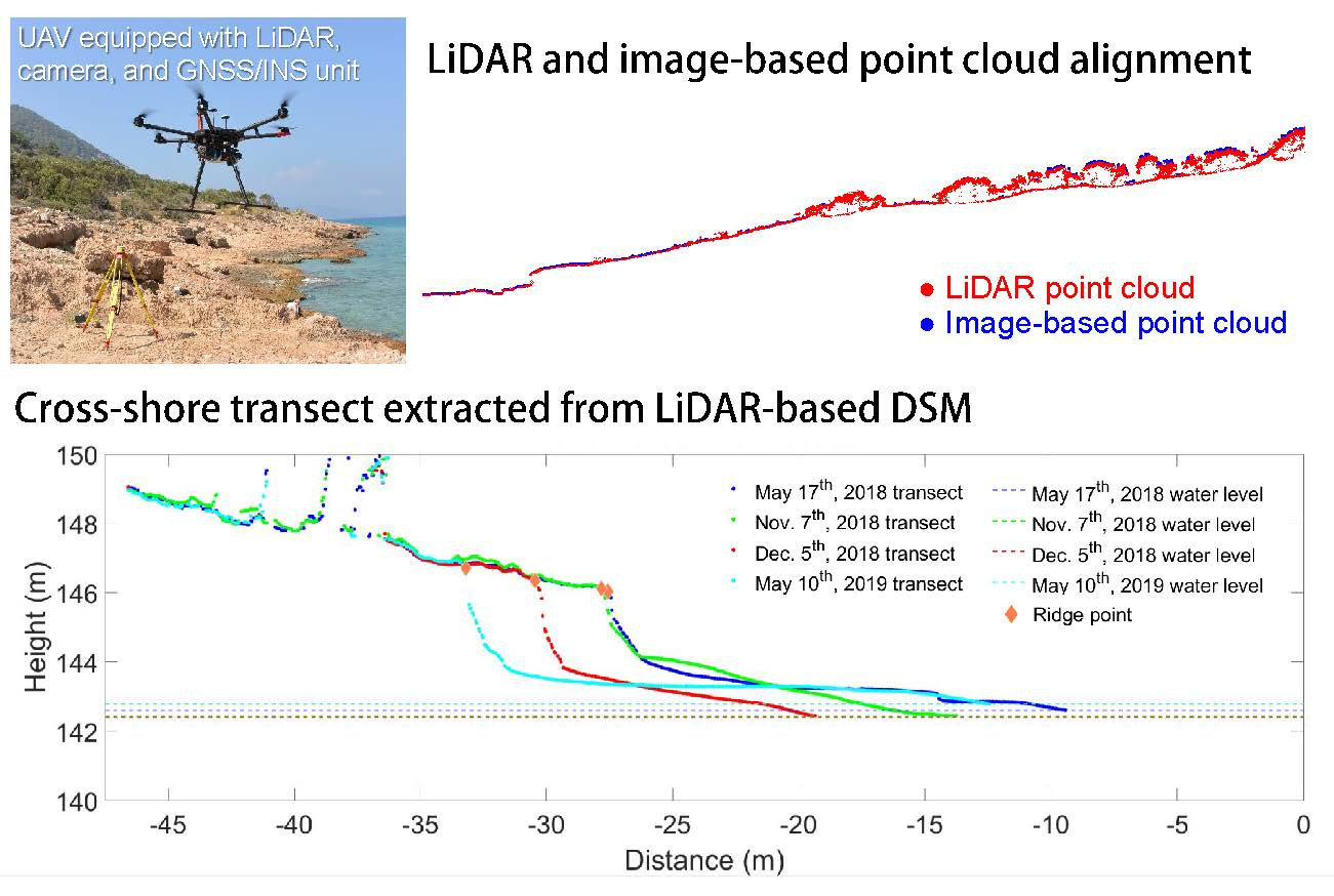
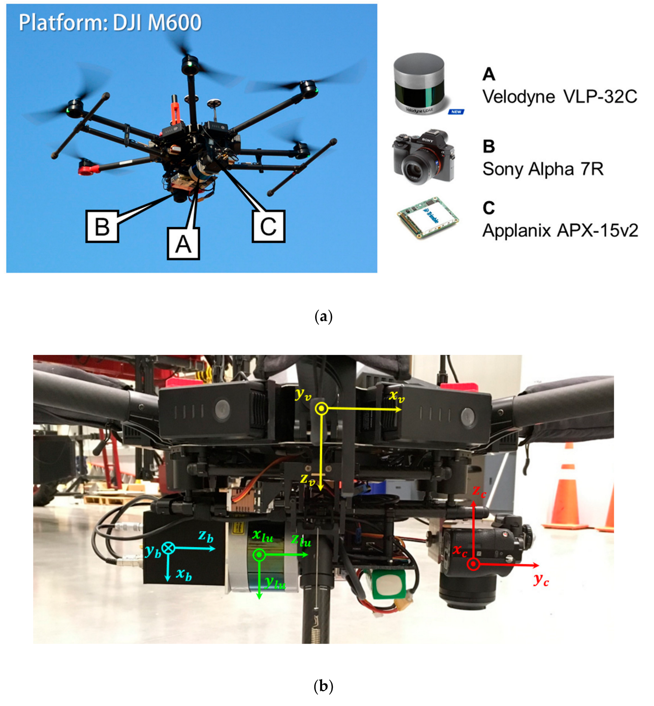
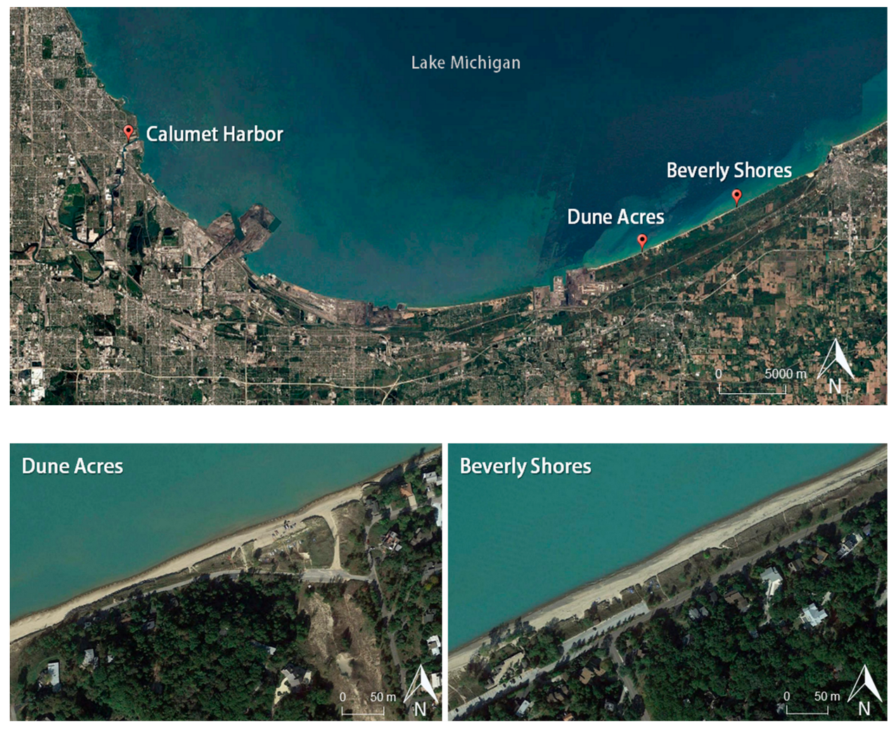
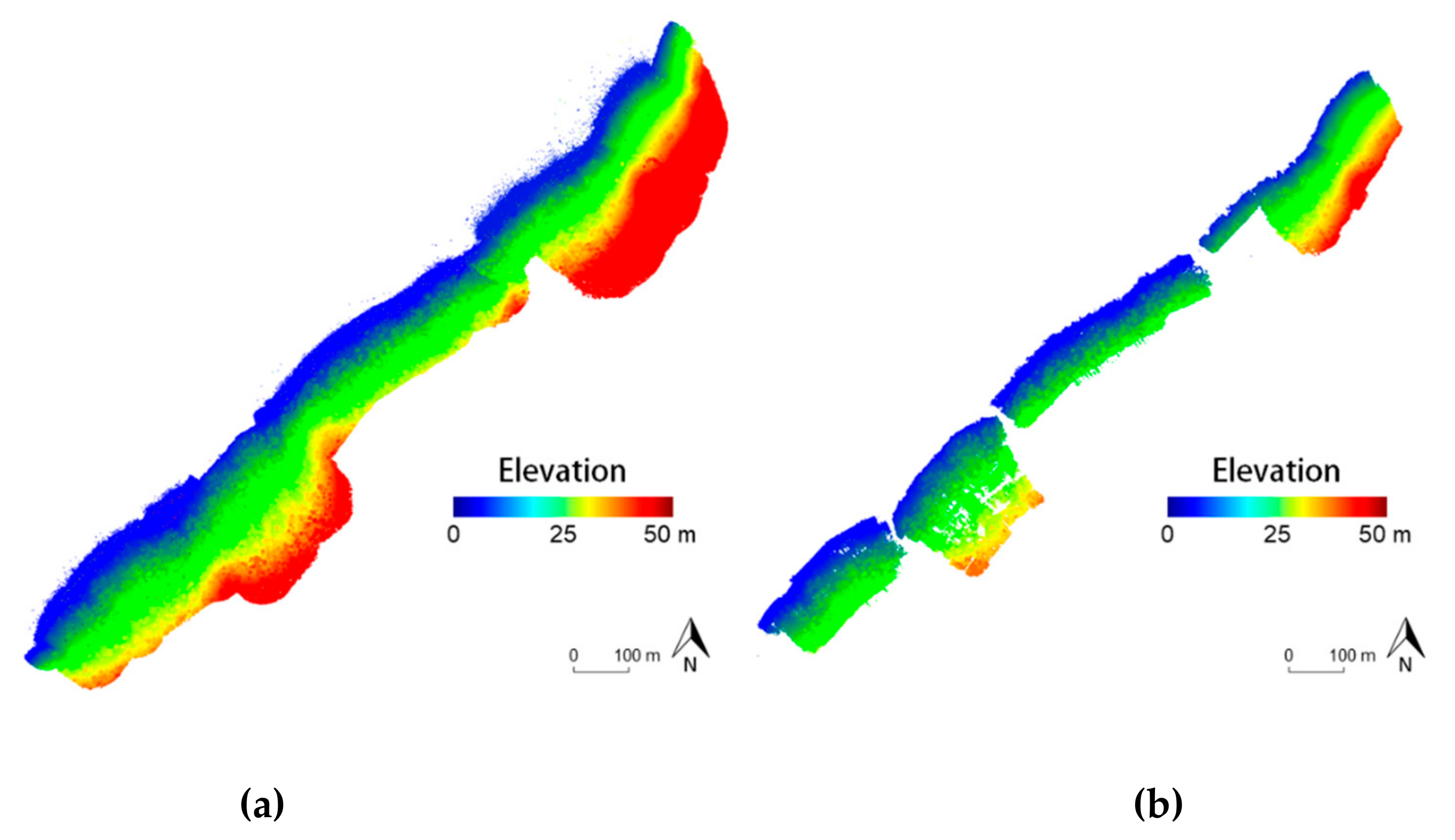
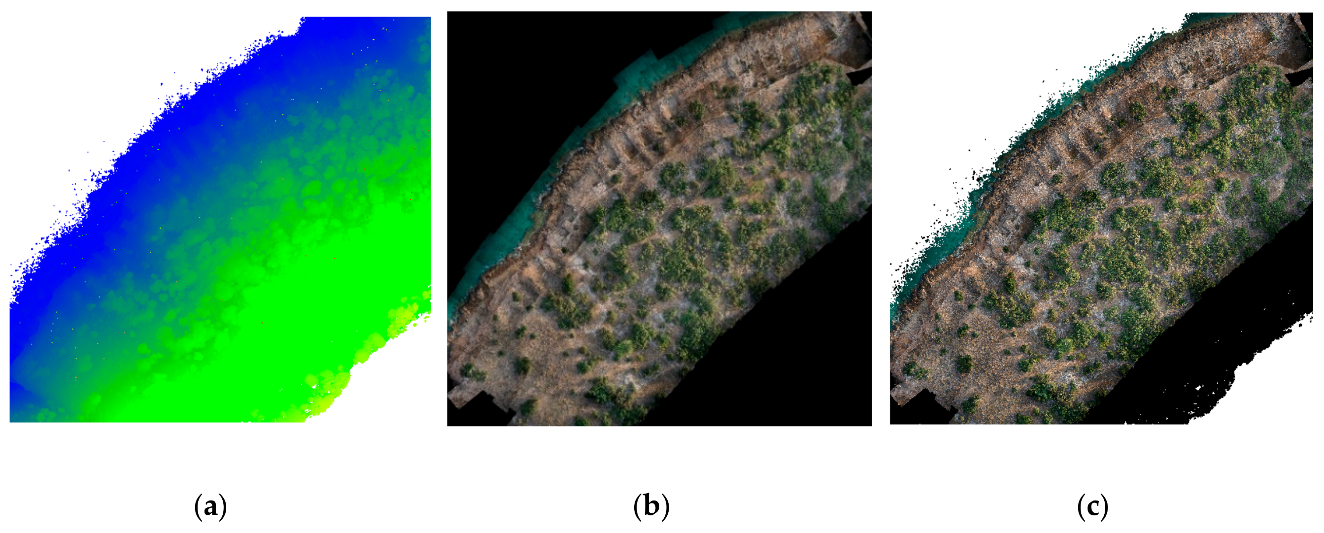
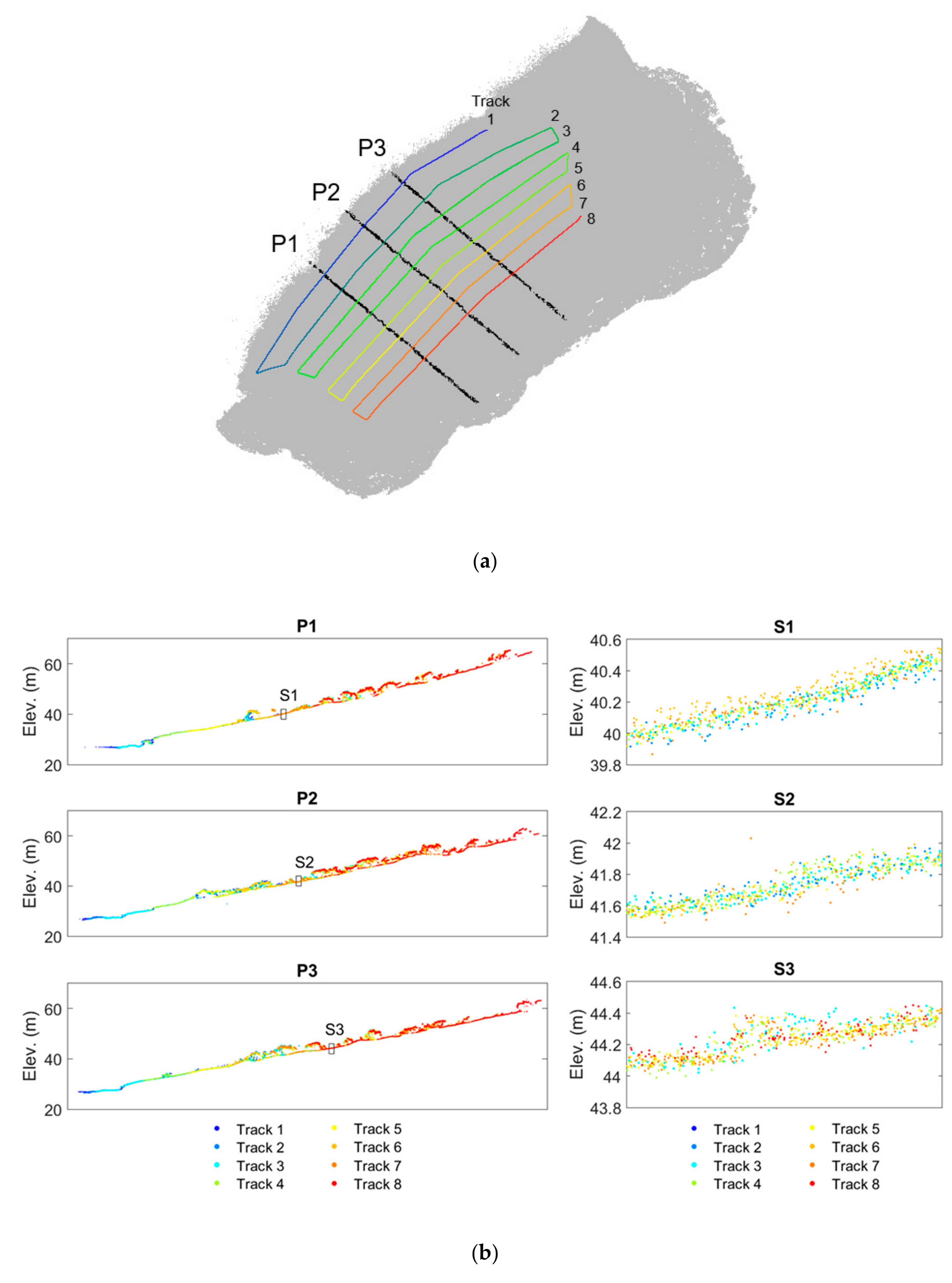
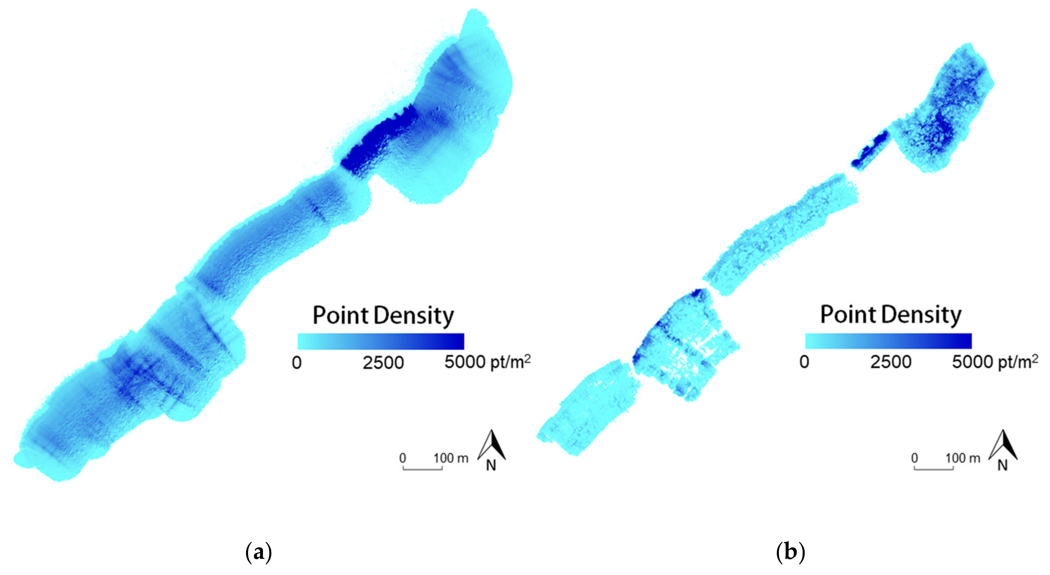
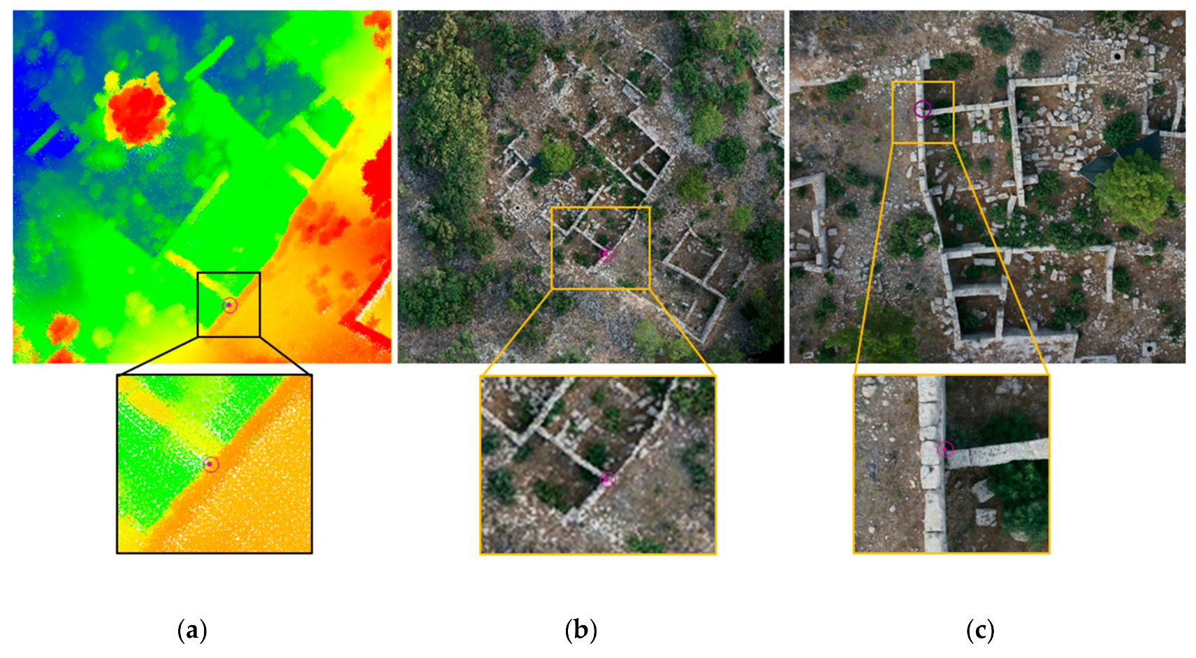
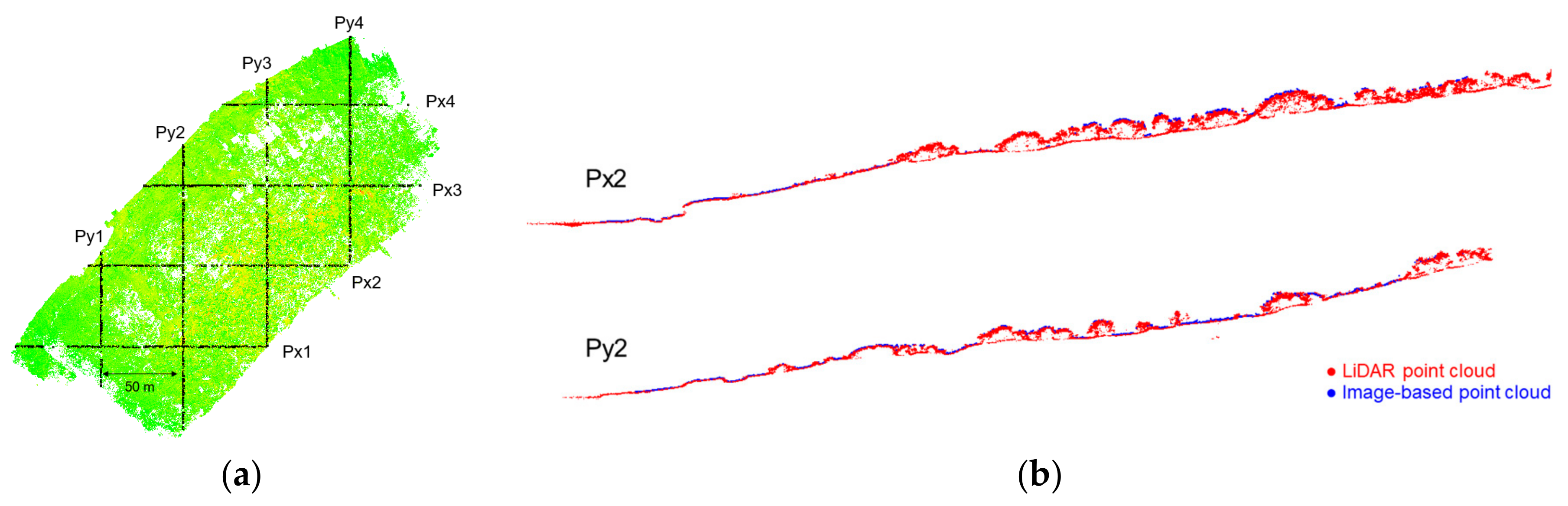
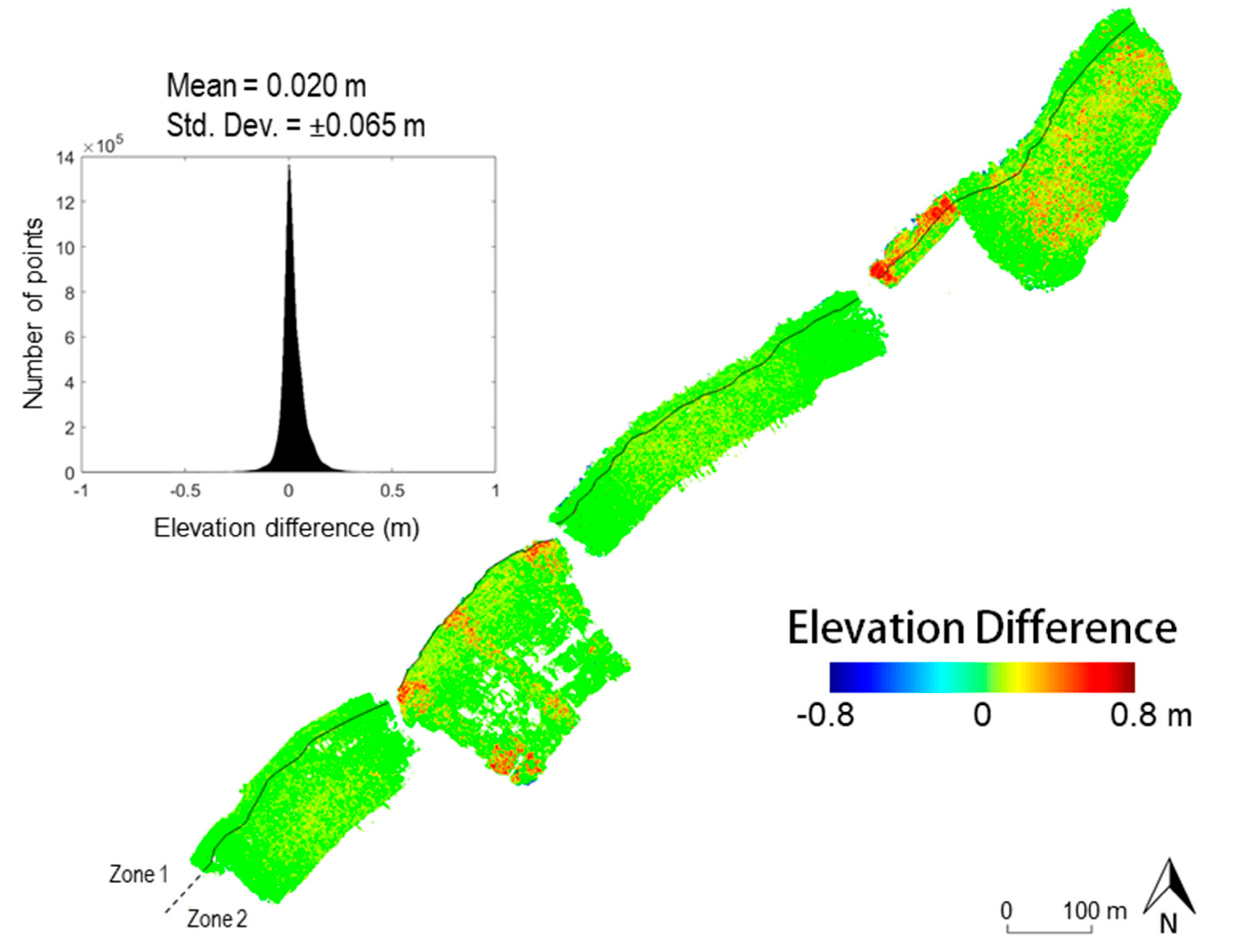
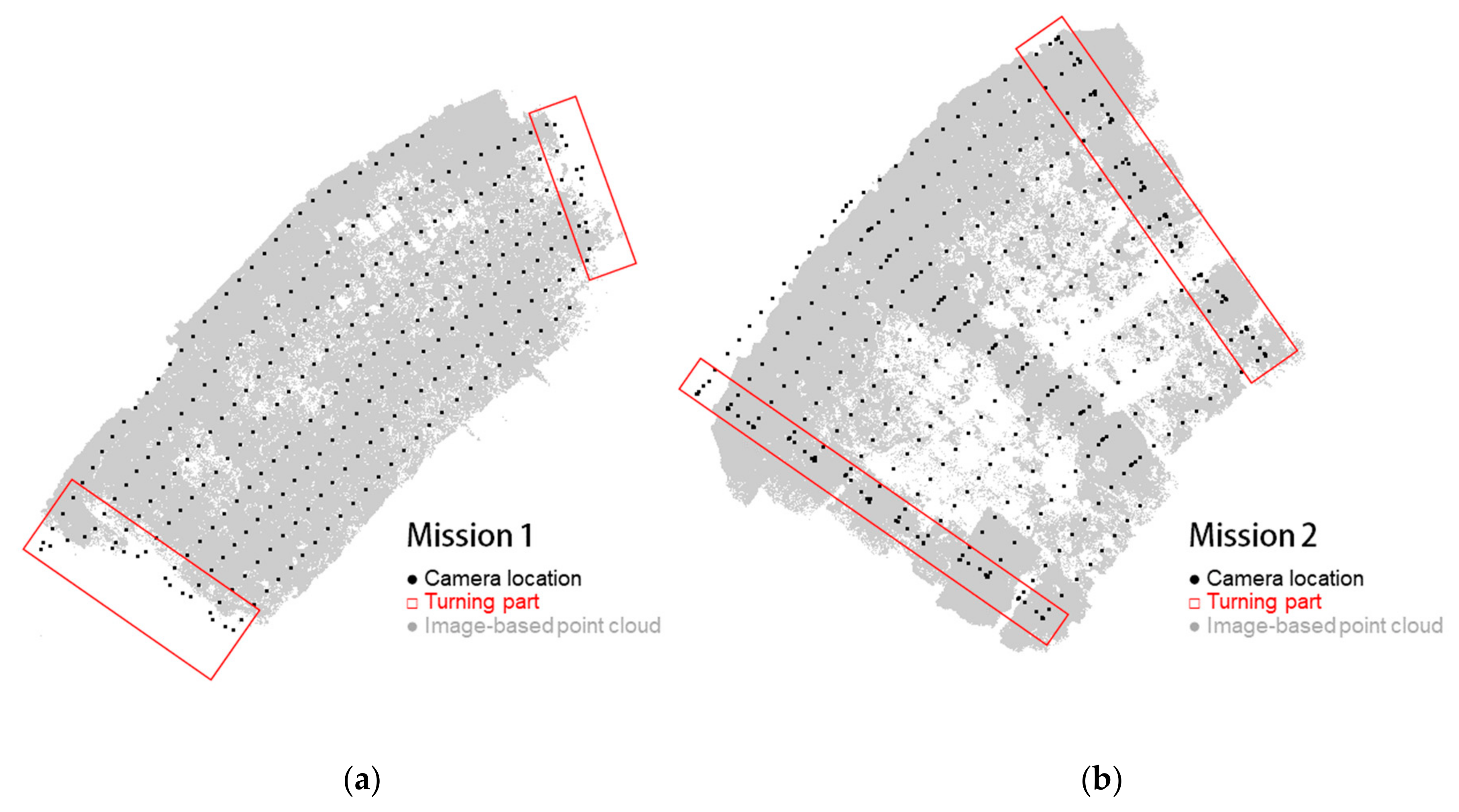
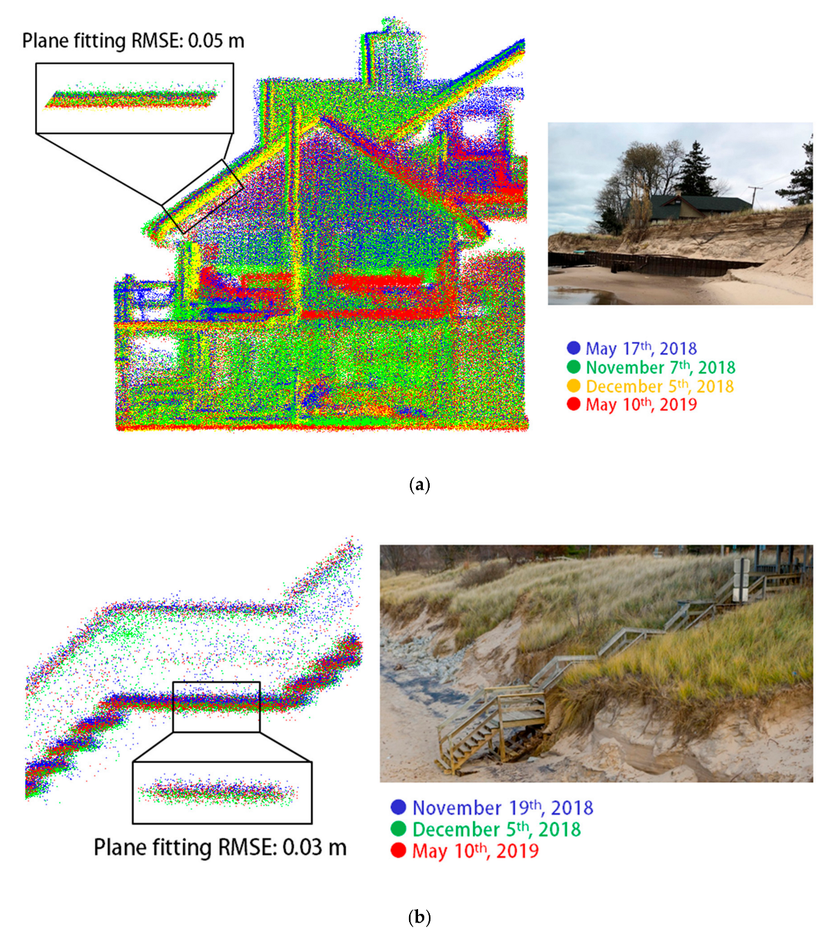
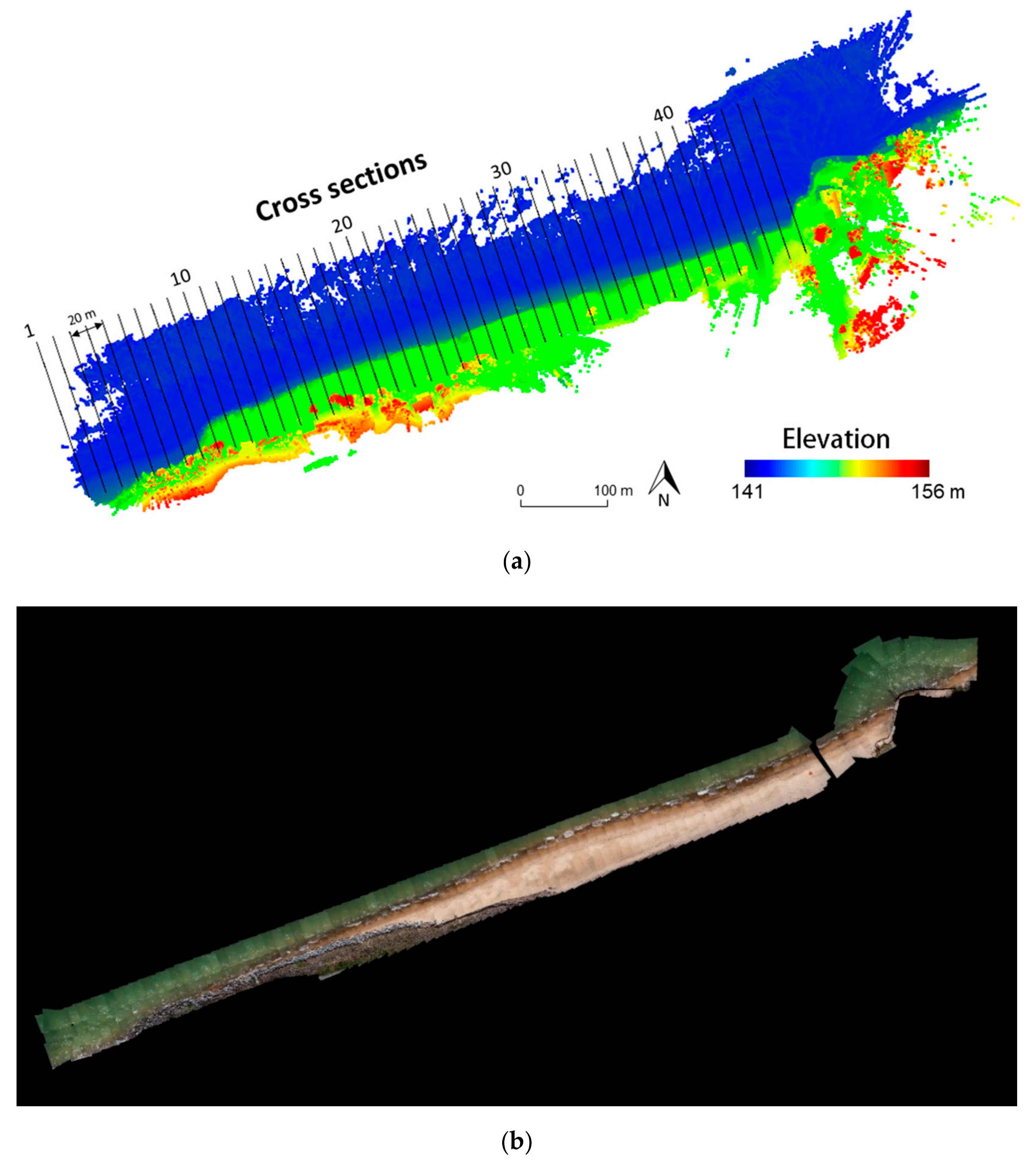
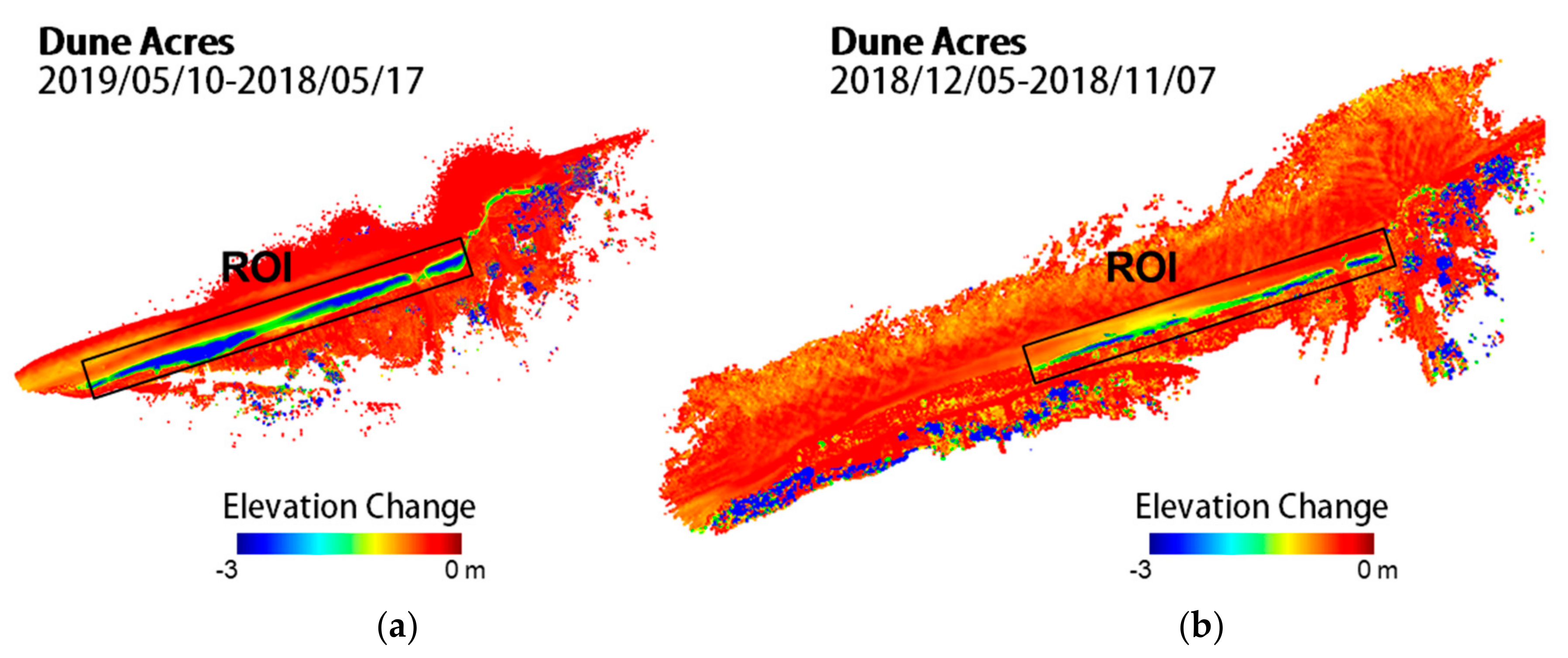
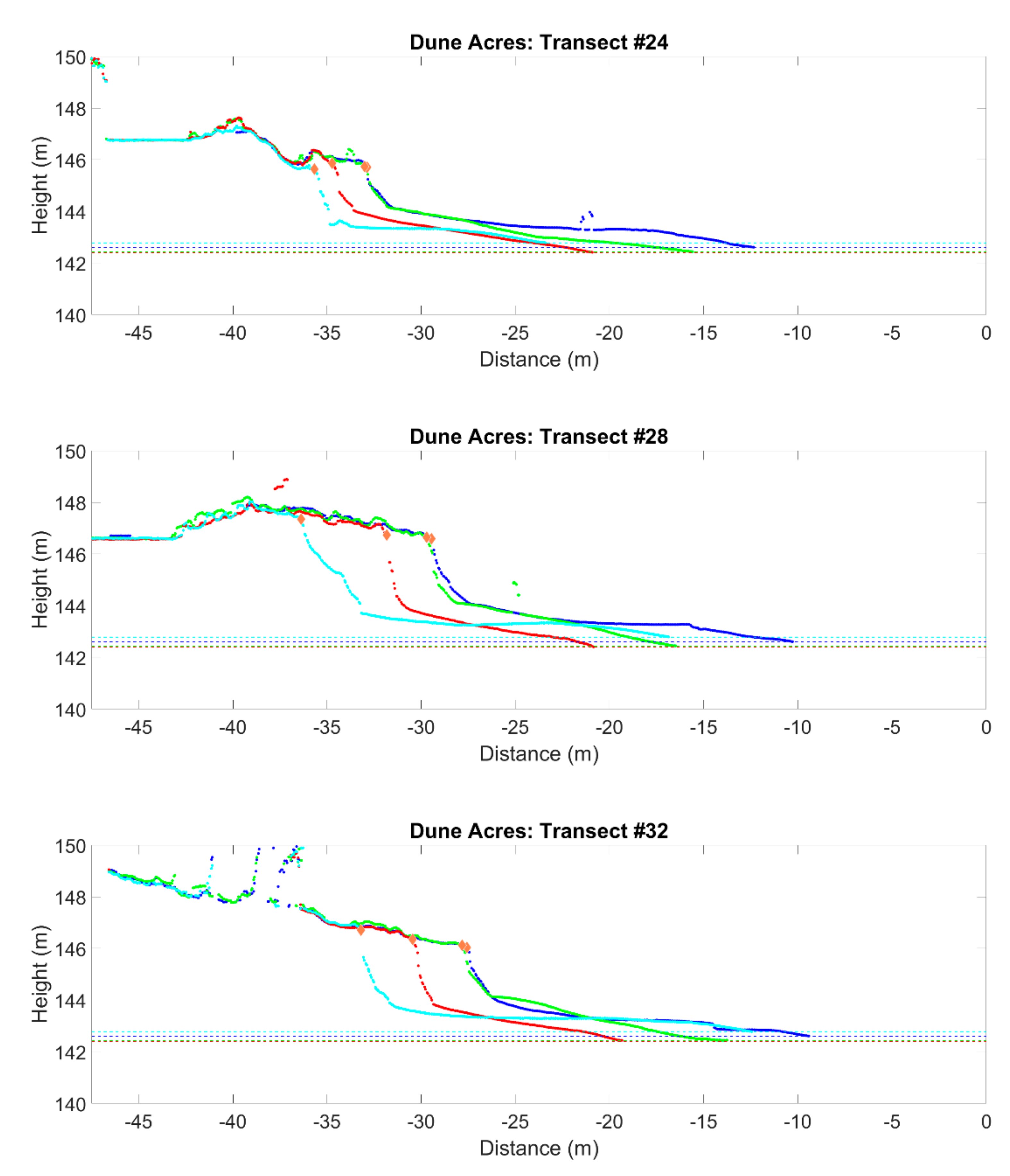
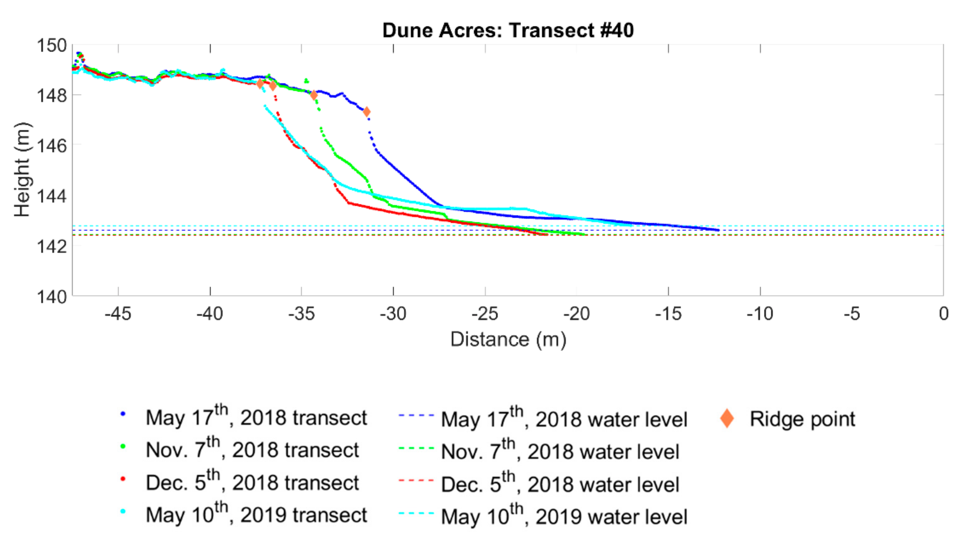
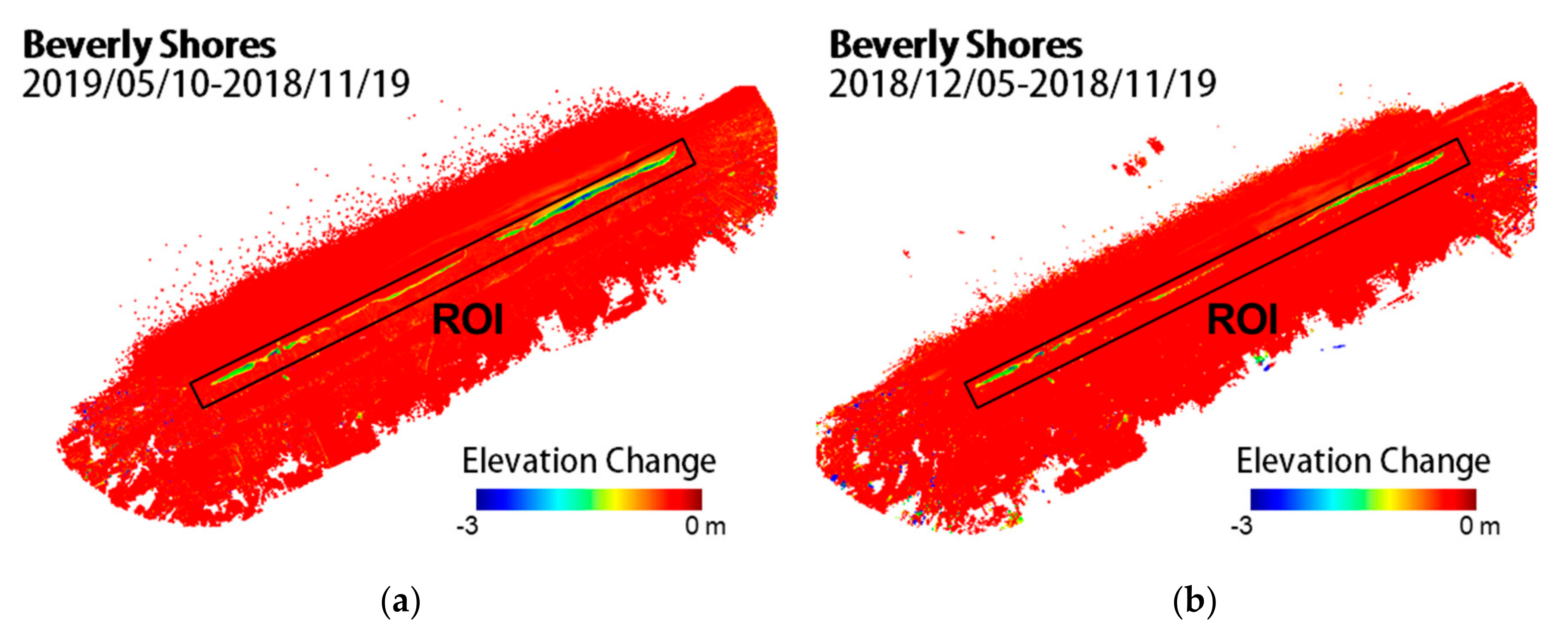
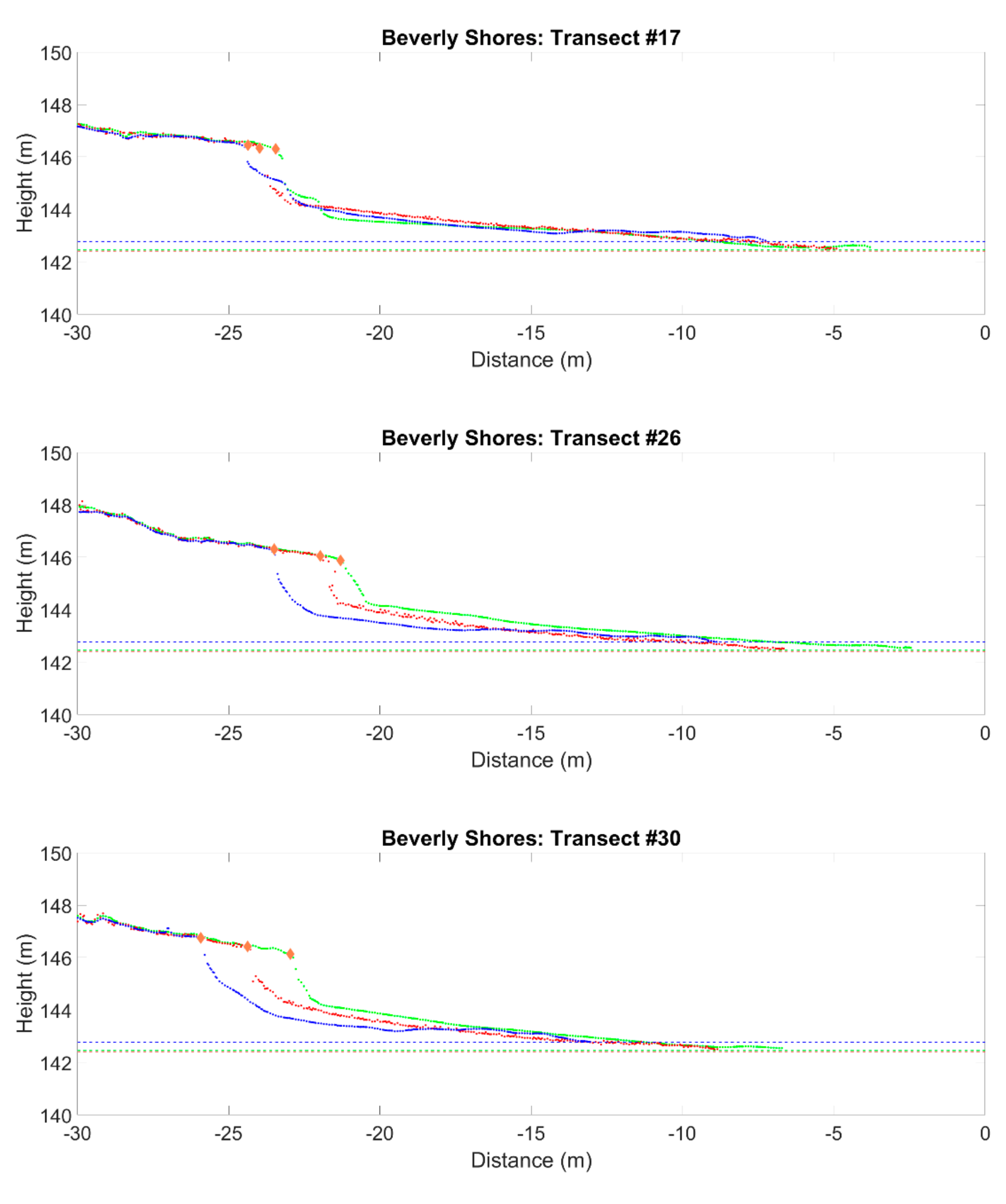
Table 1.
Merits, shortcomings, spatial resolution, and accuracy of currently existing remote sensing techniques used for coastal monitoring.
Table 1.
Merits, shortcomings, spatial resolution, and accuracy of currently existing remote sensing techniques used for coastal monitoring.
| Technique | Pros | Cons | Spatial Resolution | Accuracy | Example References |
|---|---|---|---|---|---|
| Satellite imagery |
|
| 0.46 m 2 | 2 m 2 | [7,20] |
| Aerial photography |
|
| 1 m 3 | 6 m 3 | [5,6,12,13] |
| Airborne LiDAR |
|
| 1 m 4 | Horizontal 0.50 m Vertical 0.15 m 4 | [10,11,12,13,14,15,16,17,18,19] |
| Terrestrial LiDAR |
|
| Higher than 0.1 m 5 | Centimeter-level 0.02–0.05 m | [21,22] |
| UAV photogrammetry |
|
| Higher than 0.1 m 5 | Centimeter-level 0.02–0.05 m | [23,24,25,26,27,28,29,30,31,32] |
Table 2.
Flight configurations for field surveys in Dana Island.
| Mission 1 | Mission 2 | Mission 3 | Mission 4 | Mission 5 | |
|---|---|---|---|---|---|
| Date | 28 July 2019 | 26 July 2019 | 27 July 2019 | 29 July 2019 | 29 July 2019 |
| Number of images | 590 | 514 | 597 | 663 | 587 |
| Flying height (m) | 45–50 | 45–65 | 45 | 22/40 | 50–90 |
| Average speed (m/s) | 5.5 | 6.0 | 5.0 | 3.0 | 5.0 |
| Overlap (%) | 73 | 80 | 75 | 70 | 78–88 |
| Sidelap (%) | 67 | 73 | 75 | 74 | 75–86 |
| GSD 1 (cm) | 0.63 | 0.77 | 0.63 | 0.30 | 0.70–1.20 |
| Flight time (min) | 15 | 13 | 15 | 17 | 15 |
1 Ground sample distance.
Table 3.
The shift and rotation between LiDAR-based profiles and image-based profiles.
| Profiles along X Direction | Profiles along Y Direction | ||||||
|---|---|---|---|---|---|---|---|
| ID | Horizontal Shift (m) | Vertical Shift (m) | Rotation (deg) | ID | Horizontal Shift (m) | Vertical Shift (m) | Rotation (deg) |
| Px1 | 0.0143 | 0.0590 | 0.0464 | Py1 | 0.0114 | 0.0347 | 0.0623 |
| Px2 | 0.0052 | 0.0353 | 0.0192 | Py2 | 0.0103 | 0.0182 | 0.0112 |
| Px3 | 0.0067 | 0.0472 | 0.0101 | Py3 | 0.0080 | 0.0866 | 0.0127 |
| Px4 | 0.0055 | 0.0533 | 0.0414 | Py4 | 0.0130 | 0.0550 | 0.0447 |
| Px5 | 0.0008 | 0.0072 | 0.0110 | Py5 | 0.0107 | 0.0054 | 0.0144 |
| Px6 | 0.0011 | 0.0041 | 0.0050 | Py6 | 0.0025 | 0.0133 | 0.0091 |
| Px7 | 0.0048 | 0.0503 | 0.0097 | Py7 | 0.0026 | 0.0086 | 0.0009 |
| Px8 | 0.0121 | 0.0384 | 0.0058 | Py8 | 0.0069 | 0.0328 | 0.0127 |
| Px9 | 0.0146 | 0.0590 | 0.0394 | Py9 | 0.0008 | 0.0092 | 0.0141 |
| Px10 | 0.0280 | 0.0894 | 0.0590 | Py10 | 0.0024 | 0.0522 | 0.0300 |
| Px11 | 0.0075 | 0.0124 | 0.0302 | Py11 | 0.0059 | 0.0348 | 0.0007 |
| Px12 | 0.0086 | 0.0515 | 0.0020 | Py12 | 0.0121 | 0.0658 | 0.0141 |
| Px13 | 0.0023 | 0.0525 | 0.0048 | Py13 | 0.0041 | 0.0833 | 0.0272 |
| Px14 | 0.0091 | 0.0661 | 0.0812 | Py14 | 0.0002 | 0.0498 | 0.0186 |
| Px15 | 0.0115 | 0.0146 | 0.1119 | Py15 | 0.0114 | 0.0325 | 0.0367 |
| Px16 | 0.0002 | 0.0001 | 0.0059 | Py16 | 0.0199 | 0.0173 | 0.0588 |
| Px17 | 0.0019 | 0.0107 | 0.0281 | Py17 | 0.0015 | 0.0120 | 0.0194 |
| Px18 | 0.0000 | 0.0002 | 0.0001 | Py18 | 0.0046 | 0.0012 | 0.0109 |
| Px19 | 0.0024 | 0.0110 | 0.0041 | Py19 | 0.0010 | 0.0008 | 0.0011 |
| Px20 | 0.0093 | 0.0124 | 0.0008 | Py20 | 0.0052 | 0.0292 | 0.0175 |
| Px21 | 0.0009 | 0.0102 | 0.0017 | Py21 | 0.0015 | 0.0030 | 0.0007 |
| Px22 | 0.0017 | 0.0082 | 0.0050 | Py22 | 0.0031 | 0.0179 | 0.0098 |
| Avg. | 0.0019 | 0.0139 | 0.0050 | Avg. | 0.0009 | 0.0195 | 0.0051 |
Table 4.
Elevation difference in different environments and flight missions.
| Mission 1 | Mission 2 | Mission 3 | Mission 4 | Mission 5 | All Missions | ||
|---|---|---|---|---|---|---|---|
| Zone 1 | Mean (m) | 0.006 | n/a | 0.006 | 0.031 | 0.014 | 0.014 |
| Std. Dev. (m) | 0.055 | n/a | 0.053 | 0.072 | 0.045 | 0.056 | |
| Zone 2 | Mean (m) | 0.027 | 0.019 | 0.026 | 0.030 | 0.019 | 0.021 |
| Std. Dev. (m) | 0.055 | 0.101 | 0.063 | 0.069 | 0.053 | 0.066 | |
| Overall | Mean (m) | 0.022 | 0.019 | 0.020 | 0.030 | 0.019 | 0.020 |
| Std. Dev. (m) | 0.056 | 0.101 | 0.061 | 0.070 | 0.052 | 0.065 |
Table 5.
Shoreline change measurements at Dune Acres.
| Foredune Ridge Recession (m) | Eroded Volume per m Shoreline (m3/m) | Total Eroded Volume (m3) | |||
|---|---|---|---|---|---|
| Average | Min. | Max. | |||
| May 2018November 2018 | 1.2 | 2.5 | 4.2 | 10.2 | 2243.2 |
| November 2018December 2018 | 1.2 | 0.2 | 5.6 | 12.2 | 2673.9 |
| December 2018May 2019 | 1.1 | 0.6 | 6.2 | 4.2 | 925.7 |
| Total | 5.1 | 1.6 | 8.9 | 18.2 | 3998.6 |
Table 6.
Shoreline change measurements at Beverly Shores.
| Foredune Ridge Recession (m) | Eroded Volume per m Shoreline (m3/m) | Total Eroded Volume (m3) | |||
|---|---|---|---|---|---|
| Average | Min. | Max. | |||
| November 2018December 2018 | 0.8 | 0.2 | 3.4 | 2.6 | 883.8 |
| December 2018May 2019 | 0.7 | 0.2 | 2.5 | 0.2 | 80.5 |
| Total | 1.6 | 0.2 | 4.0 | 2.8 | 938.4 |
© 2019 by the authors. Licensee MDPI, Basel, Switzerland. This article is an open access article distributed under the terms and conditions of the Creative Commons Attribution (CC BY) license (http://creativecommons.org/licenses/by/4.0/).
Share and Cite
MDPI and ACS Style
Lin, Y.-C.; Cheng, Y.-T.; Zhou, T.; Ravi, R.; Hasheminasab, S.M.; Flatt, J.E.; Troy, C.; Habib, A. Evaluation of UAV LiDAR for Mapping Coastal Environments. Remote Sens. 2019, 11, 2893. https://doi.org/10.3390/rs11242893
AMA Style
Lin Y-C, Cheng Y-T, Zhou T, Ravi R, Hasheminasab SM, Flatt JE, Troy C, Habib A. Evaluation of UAV LiDAR for Mapping Coastal Environments. Remote Sensing. 2019; 11(24):2893. https://doi.org/10.3390/rs11242893
Chicago/Turabian StyleLin, Yi-Chun, Yi-Ting Cheng, Tian Zhou, Radhika Ravi, Seyyed Meghdad Hasheminasab, John Evan Flatt, Cary Troy, and Ayman Habib. 2019. "Evaluation of UAV LiDAR for Mapping Coastal Environments" Remote Sensing 11, no. 24: 2893. https://doi.org/10.3390/rs11242893
Note that from the first issue of 2016, this journal uses article numbers instead of page numbers. See further details here.