Transferred Multi-Perception Attention Networks for Remote Sensing Image Super-Resolution

Abstract

Image super-resolution (SR) reconstruction plays a key role in coping with the increasing demand on remote sensing imaging applications with high spatial resolution requirements. Though many SR methods have been proposed over the last few years, further research is needed to improve SR processes with regard to the complex spatial distribution of the remote sensing images and the diverse spatial scales of ground objects. In this paper, a novel multi-perception attention network (MPSR) is developed with performance exceeding those of many existing state-of-the-art models. By incorporating the proposed enhanced residual block (ERB) and residual channel attention group (RCAG), MPSR can super-resolve low-resolution remote sensing images via multi-perception learning and multi-level information adaptive weighted fusion. Moreover, a pre-train and transfer learning strategy is introduced, which improved the SR performance and stabilized the training procedure. Experimental comparisons are conducted using 13 state-of-the-art methods over a remote sensing dataset and benchmark natural image sets. The proposed model proved its excellence in both objective criterion and subjective perspective.

1. Introduction

Super-resolution (SR), which aims at restoring the missing high-frequency information from lower-resolution images in order to increase the apparent spatial resolution [1], is a crucial field of research in the remote sensing community. Different from the common imaging devices (e.g., camera), imagery resolution of the space-borne imaging system is always limited by factors such as orbit altitude, revisit cycle, instantaneous field of view, optical sensor, and the like [2,3,4]. Undoubtedly, once a remote sensing satellite is launched, the super-resolving reconstruction is needed to exceed those limitations and improve the image resolution from a post-processing perspective.

SR, as a key image processing technique, has gained increasing attention for decades. Its core idea is to reconstruct a high-resolution (HR) image from its low-resolution (LR) counterpart. Many traditional algorithms have been proposed to handle this issue [4,5,6]. Recently, with the booming of deep learning-based methods and the satisfying results they gained, traditional algorithms are outperformed by them. Deep learning-based super-resolving networks could be categorized into two groups according to their structures: linear networks and skip connection-based networks.

Linear network indicates a simple single-path structure consisting of only convolutional layers without any skip connections or multiple branches. Dong et al. [7] first demonstrated that a convolutional neural network (CNN) can be used to learn mapping from LR space to HR space in an end-to-end manner. Their model, SRCNN, successfully adopts a deep learning technique into the SR community and shows outstanding performance. However, it would have to first interpolate the inputs to the desired size. This early up-sampling design is memory-intensive since the network structure parameter grows in proportion to cope with high-dimension input. Contrary to SRCNN, Shi et al. [8] proposed to perform feature extraction in LR space and increase the resolution from low-dimension space to high-dimension space only at the very end of the network. Their network, efficient sub-pixel convolutional neural network (ESPCN) [8], introduces an efficient sub-pixel convolutional layer at the end to predict a HR output from LR feature maps directly, with one up-sampler for each feature map. Their late up-sampling design significantly reduces the memory and computational requirements, but it still employs a shallow linear structure.

Considering the limited representational ability of the simple linear structure, the skip connection-based network uses residual connections to promote gradients’ propagation and makes it feasible to build very deep networks. He et al. [9] first demonstrated the advantages of the residual design. Kim et al. [10] then introduced residual learning into SR reconstruction. They pointed out that SRCNN [7] relies on the contextual information of small regions, and it converges slowly during training. Also, SRCNN works only for a single scale at a time. Therefore, they proposed a model named very deep convolutional network (VDSR) [10]. Unlike the shallow architecture used in SRCNN, VDSR exploits contextual feature priors over large image regions by cascading small size filters many times in the network. To speed up the training, it learns residuals only and uses extremely high learning rates enabled by a strategy named adjustable gradient clipping. They also extended VDSR to deal with the multi-scale super-resolving problem jointly in a single network. The deeply recursive convolutional network (DRCN) [11] is another model proposed by Kim et al., which applies the same convolutional layers multiple times, as the name indicates. Based on a similar idea of using recursive units, Tai et al. later introduced recursive block in the deep recursive residual network (DRRN) [12] and memory block in the persistent memory network (MemNet) [13]. Note that References [10,11,12,13] still require bicubic interpolated images as input. As for post-up-sampling networks, Ledig et al. [14] introduced the residual network (ResNet) [9], which is proposed to solve high-level image processing problems, such as image classification and target detection, into their model, SRResNet. Lai et al. employed a novel pyramidal framework within their network laplacian pyramid super-resolution network (LapSRN) [15], which consists of three sub-networks to predict the residual features under large SR factors in a progressive manner. Other recent work like the information distillation network (IDN) [16], adopts an information distillation block, which is made up of enhancement units and compression units. Super-resolution network for multiple degradations (SRMD) [17] takes multiple degradations into account simultaneously, which offers a unique capability. The cascading residual network (CARN) [18] uses multiple cascading connections to incorporate local-level and global-level representations. This strategy makes information and gradient propagate efficiently, but it neglects the information difference between different levels.

As for the remote sensing community, the authors of Reference [1] explored enhancing high-frequency content and image-to-image translation based on Reference [14]. Huang et al. [2] combined SRCNN [7] and VDSR [10] and achieved superior SR performance on Sentinal-2A data. Luo et al. [19] then improved the work of Reference [10] with a mirroring reflection method in the light of image self-similarity. Lei et al. [20] explored a multi-fork design, named local-global combined network, to learn multi-level feature information of remote sensing images including local details and global environmental information. Xu et al. [21] argued that Reference [20] ignores the local information produced by lower layers and further proposed the deep memory connected network [21], which employs local and global memory connections to further leverage local details and global priors learned in different convolutional layers. In fact, the image information they utilized are still limited. Furthermore, considering the insufficiency of the good-qualified HR remote sensing training samples, Huat et al. [22] studied a deep generative network to learn mapping between LR space and HR space without external HR training data. They super-resolved remote sensing images from an unsupervised perspective.

In a word, deep learning-based methods achieved significantly satisfying performance in the SR problem, and the skip-connection design further optimized the learning process and improved the hierarchical representation ability of the networks. Nonetheless, these networks still have some deficiencies when super-resolving remote sensing data.

First, the aforementioned methods forgot that all prior knowledge learned by their networks are useful for reconstructing. Even though References [18,20,21] took pattern information at the local-level and global-level into account, what they utilized is still limited. Also, none of them [7,8,10,11,12,13,14,15,16,17,18,19,20,21,22] attempt to build a model with multiple perceptual scales, which could learn information at diverse context scales adaptively. Remote sensing images have highly complex spatial distribution and the ground objects exhibited usually share diverse ranges of their scales. Therefore, extracting as much prior knowledge as possible at different levels is critical to coping with the complexity and variability of the remote sensing data and reconstructing images with high fidelity.

Second, all methods previously discussed treat the learned feature equally in the SR process, which lacks scalability in processing information at different levels. To be specific, some studies tried to learn local and global information [18,20,21] or multi-scale features [23], but they neglected the channel-wise constituent differences across those feature maps and failed to use them reasonably. Actually, information obtained from different levels are usually full of components (e.g., edges, textures, and smooth regions) with different proportions, which are unequally important for reconstructing an image.

To solve these problems, based on the idea of “the more complementary prior information we capture the better reconstructions we get”, a multi-perception attention network (MPSR) is developed for remote sensing image super-resolution. The main contribution of this study is:

• Present MPSR, a parallel two-branch structure, which achieves multi-perception learning in image patterns and multi-level information adaptive weighted fusion simultaneously.
• Propose residual channel attention group (RCAG), where the enhanced residual block (ERB) serves as the main building block to fully capture the prior information from diverse perception levels and the attention mechanism allows the group to focus on more informative feature maps adaptively.
• Train the proposed model with a supervised transfer learning strategy to cope with the lack of real HR remote sensing training samples and further boost the reconstruction ability of the proposed network toward remote sensing images.

In this article, we first analyze the proposed methods in Section 2. In Section 3, we clarify the experimental settings, demonstrate the effectiveness of the proposed methods, study the relations between SR performance and the factors such as the number of the enhanced residual blocks and the number of residual channel attention groups, and compare the proposed MPSR with recent works in objective criterion and subjective perspective. Further discussion is given in Section 4, and the conclusion is provided in Section 5.

2. Materials and Methods

2.1. Network Architecture

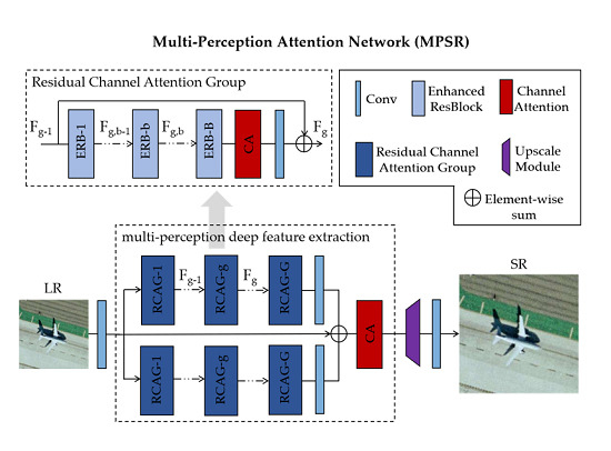
As shown in Figure 1, MPSR employs a well-designed two-branch structure, which is capable to learn a diverse set of priors at multiple context scales. Since the multi-level information obtained has varying importance for reconstruction due to the channel-wise constituent differences, the attention mechanism [24,25,26,27] is introduced to rescale it. The whole network mainly consists of three parts: shallow feature learning, multi-perception deep feature extraction, and reconstruction.

Here, the LR input image is denoted as $I_{LR}$. One convolutional (Conv) layer is used to extract shallow feature $F_0$ from $I_{LR}$. Formally, the first layer is expressed as a function $f_{SF}(\cdot )$:

$$F_0=f_{SF}(I_{LR}),$$

(1)

$F_0$ is used for multi-level information extraction. Then:

$$F_{\mathrm{ML}}=f_{MP}(F_0),$$

(2)

where $f_{MP}(\cdot )$ denotes the parallel two-branch multi-perception structure, which further contains G RCAGs in each branch. Since the proposed structure achieves learning prior information at multiple levels, its output is treated as $F_{ML}$. More details about the multi-perception part are provided in Section 2.3. $F_{ML}$ is then sent to the reconstruction part, which is composed of an upscale module and a Conv layer:

$$F_{\mathrm{UP}}=f_{UP}(F_{ML}),$$

(3)

where $f_{UP}(\cdot )$ and $F_{UP}$ denote upscale module and upscaled feature map, respectively. The sub-pixel Conv layer [8] is chosen as the upscaler, which can aggregate LR images and project them to high-dimensional space. The upscaled feature is reconstructed via the last Conv layer:

$$I_{\mathrm{SR}}=f_{REC}(F_{UP}),$$

(4)

where $I_{SR}$ indicates the reconstruction result of MPSR.

Finally, the whole SR process is defined as:

$$I_{\mathrm{SR}}=f_{MPSR}(I_{LR})=f_{REC}(f_{UP}(f_{MP}(f_{SF}(I_{LR})))),$$

(5)

where $f_{MPSR}(\cdot )$ represents the function of MPSR.

2.2. Loss Function

MPSR is optimized with loss function. There are several choices to serve as a loss function, such as $L_2$ loss, $L_1$ loss, perceptual, and adversarial losses. $L_1$ loss is chosen to be minimized, for it has been demonstrated to be more suitable for SR tasks [28]. Considering a given training dataset $\left\{{I_{LR}^{\mathrm{i}},I_{HR}^{\mathrm{i}}}_{\mathrm{i}=1}^{\mathrm{n}}\right\}$, which contains n HR training samples and their degenerated LR versions, the goal of training MPSR is to optimize the $L_1$ loss to recover from $I_{\mathrm{LR}}$, an image $I_{\mathrm{SR}}=f_{MPSR}(I_{LR})$ which is as similar as possible to the ground truth image $I_{\mathrm{HR}}$:

$$L(\Theta )=\frac{1}{n}{\displaystyle \sum _{i=1}^n||f_{MPSR}}(I_{LR}^i)-I_{HR}^i|{|}_1,$$

(6)

where $\Theta$ indicates the weight set of MPSR. More details about training are given in Section 3.1.

2.3. Multi-Perception Learning

Multi-perception learning and multi-level information adaptive weighted fusion are achieved by combining ERBs and RCAGs. Hence, details about these two basic modules are given first in the following subsections.

2.3.1. Enhanced Residual Block

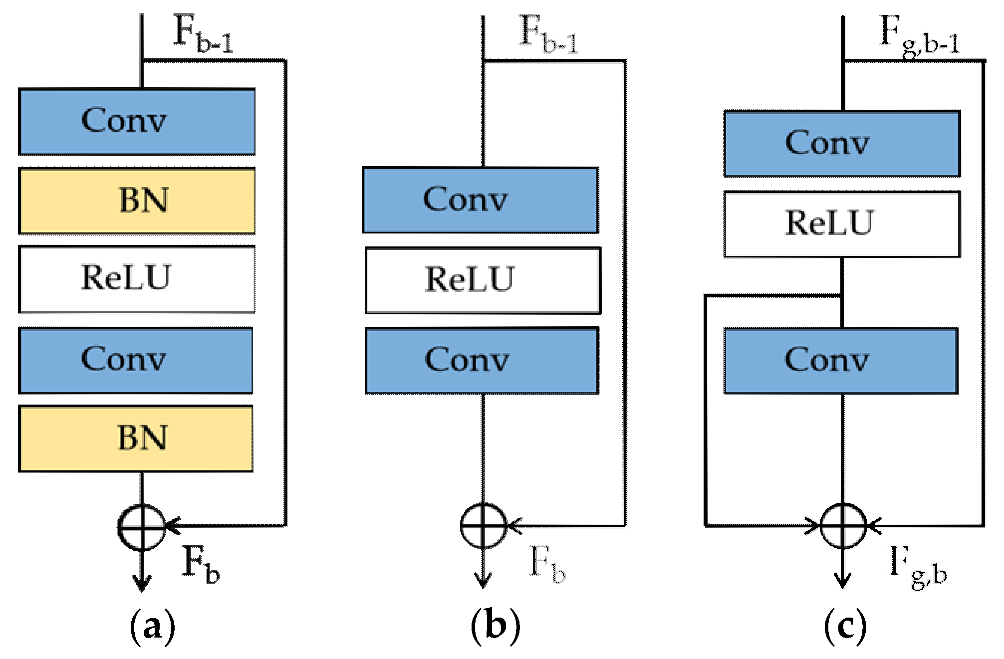
Residual designs exhibit excellent performance from low-level tasks (e.g., SR [10,11,12,13,14,16,18,19,21,22,23,25,26,27]) to high-level tasks (e.g., image classification [9]). Ledig et al. [14] successfully applied the residual block architecture (Figure 2a) [9] to resolve the SR problem without much modification. Some researchers [21,29] further removed the batch normalization (BN) layers from the residual blocks in their network (Figure 2b) and experimentally showed that this simple modification can improve the super-resolving performance. Tong et al. [30] then pointed out that skip connections between Conv layers provide an effective way to jointly employ the low-level information and high-level information to enhance the super-resolving performance.

To fully capture the feature information at different levels, we further optimized the common residual block architecture (Figure 2b) by introducing a short residual connection (Figure 2c). This block structure, named the enhanced residual block (ERB), is the basic constituent unit of the proposed RCAG introduced in Section 2.3.2.

As shown in Figure 2c, the later Conv layer in an ERB takes the output of the former Conv layer as input, assuming that filters of the same size (i.e., 3 × 3) are used for these two Conv layers. For the first layer, the receptive field is of size:

$$(2\times 1+1)\times (2\times 1+1)=3\times 3,$$

(7)

For the next layer, the size of the receptive field is:

$$(2\times 2+1)\times (2\times 2+1)=5\times 5.$$

(8)

That is, Conv layers of the same spatial size form relatively different receptive fields. Thus, two perceptual scales can be achieved in each ERB.

In general, a large receptive field means that the Conv layer can collect and analyze more neighbor pixels to predict feature maps which would contain more contextual information. In other words, the output feature maps of the later Conv layer contain more contextual feature priors, which can be exploited to predict high-frequency components, than those of the former Conv layer. Moreover, the two short residual connections within the ERB carry the input and the output of the former Conv layer to the end, that is, information from three different levels serve as the total output of an ERB (e.g., ERB_g,b, the b-th ERB in g-th RCAG):

$$F_{\mathrm{g},\mathrm{b}}=F_{g,b-1}+f_1(F_{g,b-1})+f_2(f_1(F_{g,b-1}))=f_{ER{B}_{g,b}}(F_{g,b-1}),$$

(9)

where $f_1(\cdot )$, $f_2(\cdot )$, and $f_{ER{B}_{g,b}}(\cdot )$ denote the combination of the former Conv layer and ReLU [31], the later Conv, and the function of ERB_g,b, respectively. $F_{g,b-1}$ and $F_{g,b}$ are the input and output of ERB_g,b. It should be noted that if the short residual connection added is removed, like the block structure shown in Figure 2b, the feature information generated by the former Conv layer would be discarded.

In brief, the ERB not only achieves two perceptual scales but also fully utilizes the prior information at three different levels by itself. The effectiveness of the ERB surpassing the common residual block (Figure 2b) is shown quantitatively in Section 3.2.

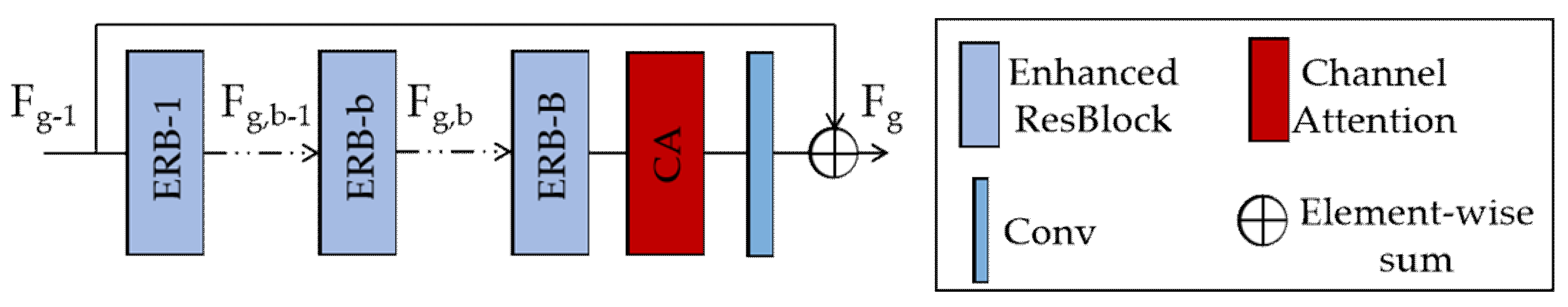
2.3.2. Residual Channel Attention Group

It has been demonstrated that stacked residual blocks and one global residual connection can be used to construct a deep network in Reference [14]. Actually, simply stacking residual blocks to build a very deep network would suffer training difficulties (e.g., vanishing gradients) and can hardly achieve performance improvements. Therefore, a residual channel attention group (RCAG) structure is proposed here.

As shown in Figure 3, one RCAG (e.g., RCAG_g, the g-th RCAG in a branch) contains B ERBs. As discussed in Section 2.3.1, the b-th ERB in RCAG_g can be formulated as:

$$F_{\mathrm{g},\mathrm{b}}=f_{ER{B}_{g,b}}(F_{g,b-1})=F_{g,b-1}+f_1(F_{g,b-1})+f_2(f_1(F_{g,b-1})),$$

(10)

where $F_{g,b-1}$, the input of ERB_g,b, is composed of responses generated by ERB_g,b-1.

Specifically, each ERB in RCAG_g receives three different levels of image information output by the former ERB and generates information at three other levels as the input of the later ERB, except ERB_g,1. The multi-level feature information obtained by all stacked ERBs in RCAG_g can be described as:

$$F_{{\mathrm{ERBS}}_{\mathrm{g}}}=F_{\mathrm{g},\mathrm{B}}=f_{ER{B}_{g,\mathrm{B}}}(F_{g,B-1})=f_{ER{B}_{g,\mathrm{B}}}(f_{ER{B}_{g,B-1}}(\dots f_{ER{B}_{g,1}}(F_{g-1})\dots )),$$

(11)

where $F_{g-1}$ represents the input of RCAG_g, and the output of RCAG_g-1.

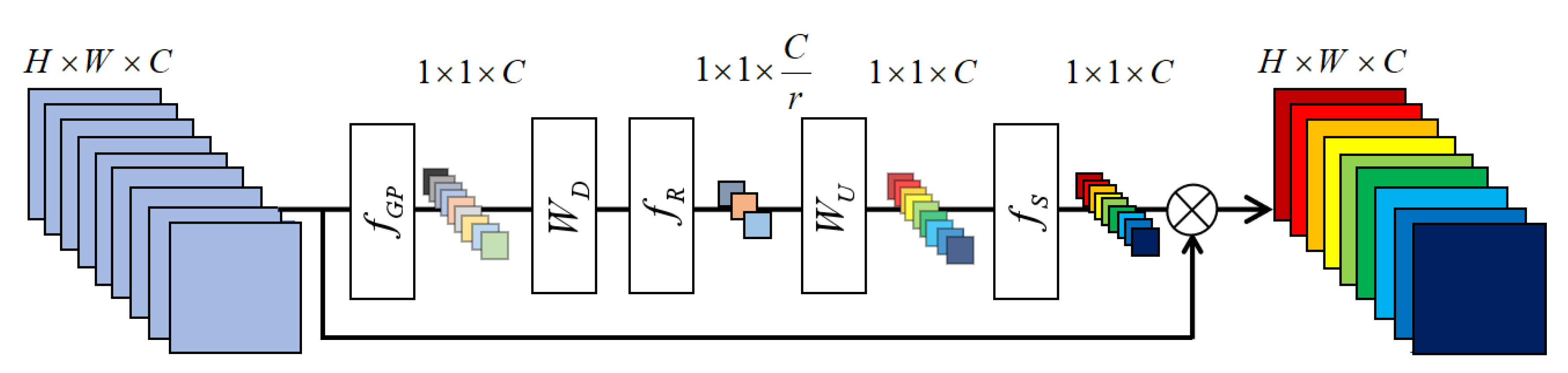
Considering channel-wise differences among the obtained multi-level information $F_{{\mathrm{ERBS}}_{\mathrm{g}}}$, the attention mechanism [24,25,26,27] is further integrated into every RCAG.

The channel attention (CA) mechanism [27] generates different attention for each channel-wise feature map it receives. As shown in Figure 4, the input, which contains C feature maps of a size H × W. Vector $z\in R^C$, a channel-wise statistic of size 1 × 1 × C, can be obtained by performing global average pooling to $X.$ The c-th element of $z$ is determined by:

$$z_c=f_{GP}(x_c)=\frac{1}{H\times W}{\displaystyle \sum _{i=1}^H{\displaystyle \sum _{j=1}^W{x}_c(i,j)}},$$

(12)

where $x_c(i,j)$ denotes the pixel value at position $(i,j)$ of the c-th feature map $x_c$ and $f_{GP}(\cdot )$ represents the global average pooling function. Such channel-wise statistic, $z=[z_1,\dots ,z_c\dots ,z_C]$, can be viewed as a collection of the local descriptors, whose statistics contribute to the expression of the whole image [24,27].

As studied in References [26,27], a gating mechanism with sigmoid function is adopted to extract channel-wise dependencies from the information aggregated by the global average pooling function:

$$s=f_S(W_U\otimes f_R(W_D\otimes z)),$$

(13)

where $f_S(\cdot )$ and $f_R(\cdot )$ indicate the sigmoid function and ReLU, respectively. $W_D$ denotes the weights of a Conv layer, which serves as channel-downscaler with a reduction ratio, $r$[27]. After channel-downscaling and being activated by $f_R(\cdot )$, the low-dimension vector $z_1=f_R(W_D\cdot z)$ of size 1 × 1 × C/r is later upscaled with factor $r$ by a channel-upscaling Conv layer, whose parameter set is $W_U.$ Finally, the statistic $s=[s_1,\dots ,s_c\dots ,s_C]$ is outputted by sigmoid gating $f_S(\cdot )$, which is employed to perform channel-wise rescaling to the input $X$:

$${x^{\prime }}_c=s_c\cdot x_c,$$

(14)

$$X^{\prime }=[{x^{\prime }}_1,\dots ,{x^{\prime }}_c\dots ,{x^{\prime }}_C],$$

(15)

where ${x^{\prime }}_c$ is the rescaled c-th feature map.

In this case, the multi-level information obtained by all stacked ERBs in a RCAG can be adaptively rescaled with the CA mechanism by considering constituent differences among channels. The function of CA is denoted as $f_{CA}(\cdot )$, and could further have:

$${F^{\prime }}_{{\mathrm{ERBS}}_{\mathrm{g}}}=f_{CA}(F_{ERB{S}_g}).$$

(16)

Then, the total output of RCAG_g is formulated as:

$$F_{\mathrm{g}}=f_{RCA{G}_g}(F_{g-1})=F_{g-1}+Conv({F^{\prime }}_{ERB{S}_g}).$$

(17)

As discussed above, a RCAG achieves multi-level information extraction and adaptive weighted fusion by combining B stacked ERBs and a CA module. Moreover, with this modular design, the network depth can be easily controlled by modifying the number of blocks or groups. The quantitative comparison between the performance of RCAG and simple residual group (residual group composed of stacked residual blocks, without CA) is provided in Section 3.2.

2.3.3. Multi-Perception Learning Overview

Reviewing Figure 1, the proposed multi-perception deep feature extraction part has two branches. Each branch has G RCAGs and one RCAG further contains B ERBs.

As analyzed in the previous two subsections, B stacked ERBs in one RCAG have B × 2 different perceptual scales in all. RCAGs in one branch share different receptive fields with each other due to the depth they are located. Furthermore, the kernel size of all filters located in the upper-branch is set to 3 × 3 while all filters located in the lower-branch are of size 5 × 5. Also, every Conv layer in the two branches has its own scale-specific receptive field. Further enhancement of the perception capacity can be done by adding a branch in which the kernel size is larger, or by increasing the network depth. For example, kernel 7 × 7, the parameter number of one ERB is 5.44 times and 1.96 times larger than an ERB of kernel 3 × 3 and 5 × 5, respectively [32]. Adding a branch with larger convolution kernel size will introduce a great number of additional parameters, then, overfitting can arise [11]. Hence, the network ability is improved by adding modules, as shown in Section 3.2. As a result, the whole two-branch multi-perception part achieved a diverse set of perceptual scales that sums to:

$$N=2\times (G\times (B\times 2+1)+1).$$

(18)

The final multiple levels prior information $F_{ML}$ learned by MPSR is expressed as:

$$F_{ML}=f_{CA}(F_0+f_{branc{h}_1}(F_0)+f_{branc{h}_2}(F_0)),$$

(19)

$$f_{branc{h}_1}(F_0)=C\mathrm{onv}(F_{G_1}){|}_{3\times 3}=C\mathrm{on}v(f_{RCA{G}_G}(\dots f_{RCA{G}_1}(F_0)\dots )){|}_{3\times 3},$$

(20)

$$f_{branc{h}_2}(F_0)=C\mathrm{onv}(F_{G_2}){|}_{5\times 5}=C\mathrm{on}v(f_{RCA{G}_G}(\dots f_{RCA{G}_1}(F_0)\dots )){|}_{5\times 5},$$

(21)

where $f_{branc{h}_1}(\cdot )$ and $f_{branc{h}_2}(\cdot )$ are functions of the upper-branch and the lower-branch, respectively. $F_{G_1}$ and $F_{G_2}$ represent the output information of the G-th RCAG in the upper-branch and the lower-branch, correspondingly.

With this multi-perception design, the proposed network can consider feature representations from diverse receptive fields by different attention when reconstructing an image.

2.4. Transfer Training Strategy

Currently, there is no standard training set used for image SR reconstruction in the remote sensing community. As a matter of fact, it is difficult to collect a large amount of remote sensing images with clear edges and textures which are suitable for training a SR model. However, the performance of deep learning-based SR methods always benefits from a sufficient volume of good-qualified HR and LR training sample pairs. Thus, a transfer training strategy to deal with the insufficiency of training samples is introduced here. The core of transfer learning is assuming that individual models for related tasks share parameters or prior distributions of hyperparameters [33], which means to solve tasks in one domain based on the shared knowledge obtained from other related domains.

Hence, the proposed MPSR is pre-trained with the natural image set DIV2K [34] as an external knowledge set when conducting experiments. Generally speaking, the low-level feature information learned from DIV2K (e.g., point-like components, local texture and color, and point-line distribution) can be shared. In order to learn high-level feature information specific to remote sensing data, the pre-trained network is re-trained by using images randomly selected from UC MERCED [35] (a remote sensing scenes classification dataset). This training strategy further boosts the model performance on super-resolving remote sensing images. Relevant experimental results are provided in Section 3.2.

3. Results

3.1. Experiment Settings

In this section, the experiment settings on datasets, degradation model, training, and evaluation metrics are clarified.

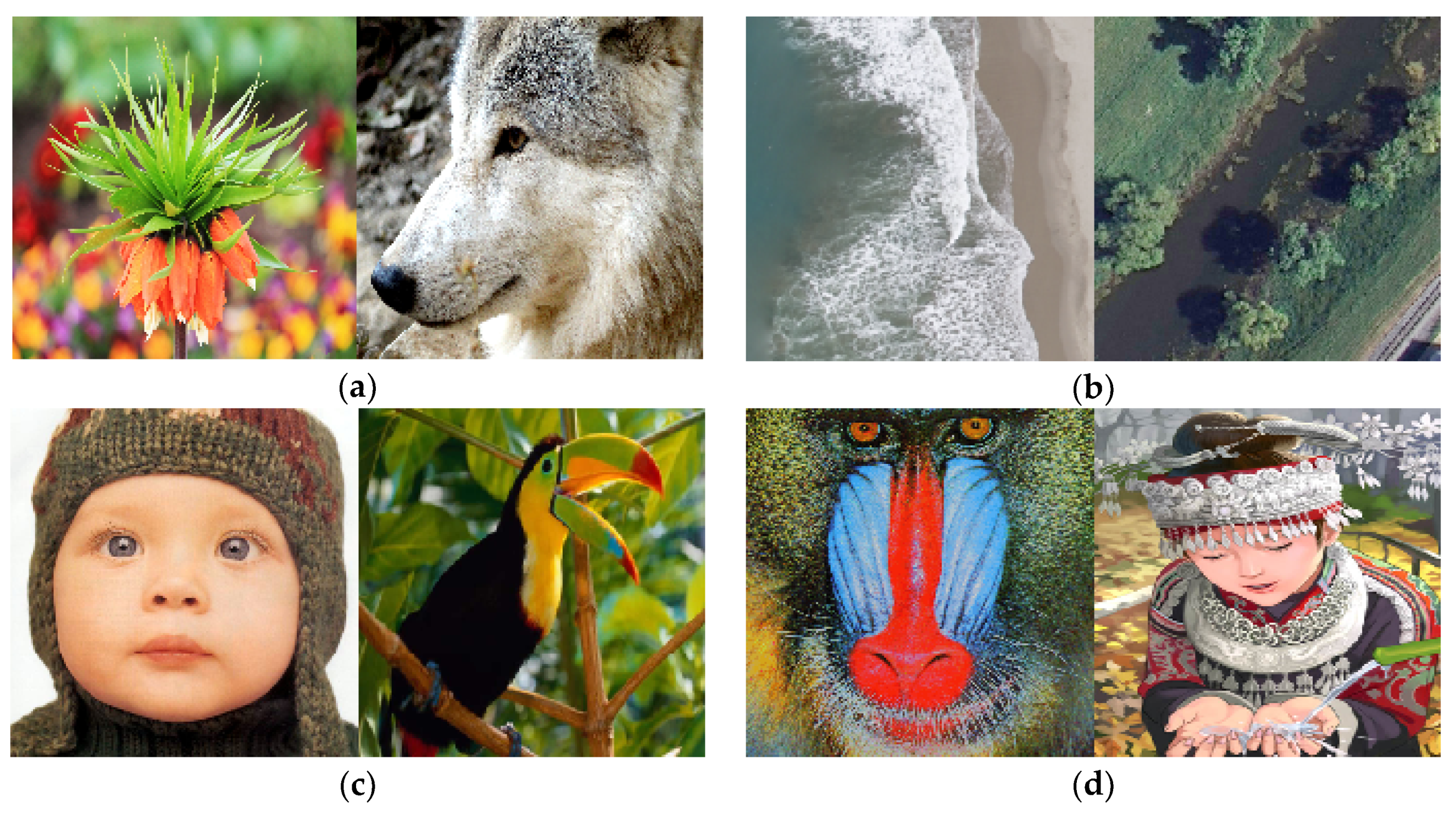
Datasets: 800 training samples from the DIV2K dataset [34] are used as the pre-training set, and 800 images are selected randomly from the UC MERCED [35] for transfer training. For testing, 120 images from the UC MERCED are chosen at random, which are different from transfer training samples, to form a test set named UCtest. To further demonstrate the effectiveness of the proposed model, it is compared with the state-of-the-art algorithms on publicly available benchmark natural datasets, including Set5 [36], Set14 [37], BSD100 [38], and Urban100 [39]. The representative images from these datasets are shown in Figure 5.

• DIV2K [34] contains 800 natural images for training. The image resolution is of around 2K.
• UC MERCED [35] contains 2100 images in size of 256 × 256 pixel. The pixel resolution is 0.3 m.
• Set5 [36] is a classical dataset which only consists of 5 test images.
• Set14 [37] has 14 test images which contain more categories compared to Set5.
• BSD100 [38] has 100 rich and delicate images ranging from natural to object-specific.
• Urban100 [39] is a relatively more recent dataset composed of 100 images, the focus of which is on urban scenes.

Degradation model: Experiments are conducted with the bicubic interpolation degradation model and three down-sampling scales (×2, ×3, ×4) [17]. Specifically, a LR version is generated from its corresponding HR counterpart by bicubic interpolation with a specific downscaling factor. For example, a three-fold down-sampling LR image can be generated from its corresponding HR counterpart by bicubic interpolation with a factor of 1/3.

Training: Data augmentation is performed on both 800 pre-training images and 800 transfer training images, including rotation of 90°, 180°, 270°, and horizontal flipping [27]. In each training batch, 16 LR input patches of size 48 × 48 and the corresponding HR patches are used. The proposed model is trained with the Adam optimizer [40] by setting β₁ = 0.9, β₂ = 0.999, and ϵ = 10^-8 [27]. The learning rate is initially set as 10^-4 and decreases to half every 2 × 10⁵ batches [26].

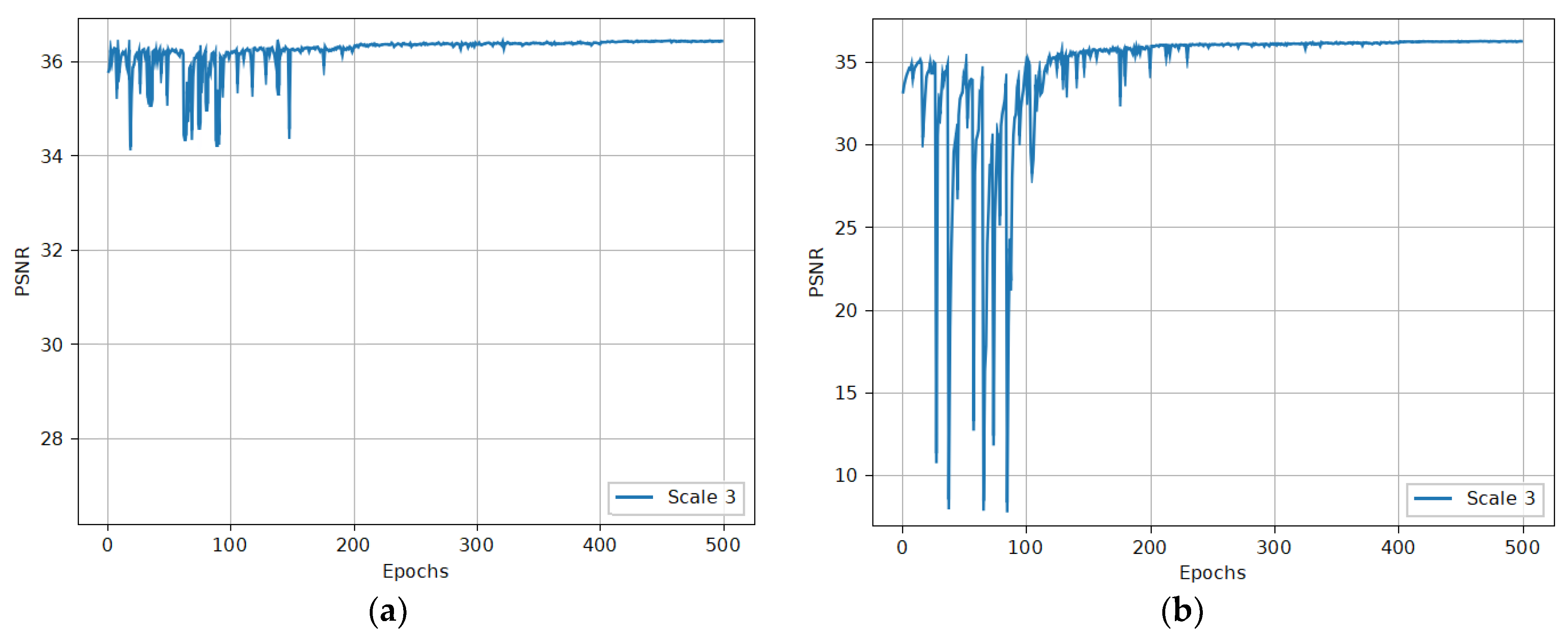
All models go through 500 epochs of pre-training, and 100 epochs of transfer training. The ×2 network is trained from scratch. After it is converged, it is used as a pre-trained model for factors ×3 and ×4 [29]. As shown in Figure 6, this pre-training strategy stabilizes the training process and further improves the network performance.

The proposed models are implemented with PyTorch [41] and 4 NVIDIA GTX 1080Ti GPUs.

Evaluation metrics: Experimental results are quantitatively evaluated with peak signal- to-noise ratio (PSNR) and the structural similarity index (SSIM) [42] on the Y channel (i.e., luminance) in transformed YCbCr space. This is due to human vision being more sensitive to details in intensity space than in color [10]. Higher PSNR and SSIM values represent better reconstruction quality.

3.2. Model Design and Performance

The effectiveness of using ERB, RCAG, and the transfer training strategy, as well as the relations between SR performance and factors, such as the number of ERBs and RCAGs, are studied in this section. Additionally, the configuration details of the final model are specified.

ERB and RCAG: To demonstrate the effects of these two proposed structures, the networks are set with B = 6 (the number of ERBs) and G = 3 (the number of RCAGs). In

Table 1. Investigations of the proposed ERB, RCAG, and transfer training strategy. The average PSNR (dB) of ×2 test results on UCtest is observed.

ERB	RCAG	Transferred	PSNR
×	×	×	39.510
√	×	×	39.540
√	√	×	39.604
√	√	√	39.728

ERB and RCAG represent the proposed enhanced resiudal block and residual channel attention group, respectively.

, the first row represents MPSR composed of a common RB (residual block with only one short residual connection, as shown in Figure 2b) and RG (residual group composed of stacked residual blocks, without CA), the PSNR value it gained is relatively low (39.510 dB). After adding ERB, the performance reached 39.540 dB, as shown in the second row. After adding RCAG, a similar trend is observed—the performance improved from 39.540 dB to 39.604 dB. These findings firmly demonstrate the effectiveness of widely extracting and reasonably leveraging multi-level prior information by introducing the proposed ERB and RCAG.

Transfer training: MPSR with 6 ERBs and 3 RCAGs is used to verify the significance of adopting the transfer learning strategy mentioned in Section 2.3. As shown in Table 1, after transfer training, the gain of MPSR-transferred (row 4) over MPSR-notransfer (row 3) reaches 0.124 dB. This improvement shows that the transferred MPSR achieves better reconstruction performance.

ERB number and RCAG number: B (the ERB number) and G (the RCAG number) of MPSR-notransfer is modified progressively to obtain the most suitable values of B and G. First, G is set to three. In terms of the results shown in

Table 2. The results of using different ERB numbers in MPSR-notransfer (G = 3). The average PSNR (dB) and average running time (sec) on UCtest (×2 test results) is observed. Best results are in bold.

	B = 6	B = 7	B = 8	B = 9	B = 10
PSNR	39.604	39.621	39.627	39.570	39.573
TIME	0.14	0.16	0.18	0.20	0.21

, B is set to eight to get a reasonable trade-off between reconstruction performance and speed. The changed value of G is shown in

Table 3. The results of using different RCAG numbers in MPSR-notransfer (B = 8). The average PSNR (dB) and average running time (sec) on UCtest (×2 test results) is observed. Best results are in bold.

	G = 3	G = 4	G = 5
PSNR	39.627	39.608	39.630
TIME	0.18	0.23	0.28

.

Generally, the reconstruction performance would further improve if the network depth kept on increasing, i.e., adding more ERBs and RCAGs, at the cost of training time. Actually, not only the running time is sacrificed but also the GPU memory usage due to the huge amount of calculations and parameters. In the end, a trade-off is made between the performance and speed for the model: i.e., B = 8 and G = 5.

Final model configuration: With regard to the final model, G is set to five in each branch and B is set to eight in each RCAG. The kernel size of channel-downscaling the Conv layer and channel-upscaling the Conv layer in the CA module are 1 × 1. The kernel size of Conv layers in the lower branch is 5 × 5 (as described in Section 2.3.3), and the kernel sizes of all the rest of the Conv layers in the network are 3 × 3. For Conv layers with filters of 3 × 3 and 5 × 5, the zero-padding strategy [10] is used to keep the sizes of all feature maps the same. Furthermore, all Conv layers in the shallow feature extraction part and multi-perception deep feature extraction part have 64 filters (C = 64), expect for the channel-downscaling layers. The filter number of channel-downscaling Conv layers as C/r is set to four, which indicates that the reduction ratio $r$ mentioned in Section 2.3.2 is 16. The setting of this value is similar to that in References [24,27]. As for the reconstruction part, the sub-pixel Conv layer [8] is used as an upscaler, and the last Conv in the network has 3 filters in order to output color images. In the following experiments, the final model without transfer training is named as MPSR, and the transferred one as MPSR-T.

3.3. Comparisons to State-of-the-Art Methods

In this section, the quantitative and qualitative results of the final model in comparison to recent state-of-the-art models, on the remote sensing dataset [35], benchmark natural image sets [36,37,38,39], and data from GaoFen-1 satellite and GaoFen-2 satellite, are provided.

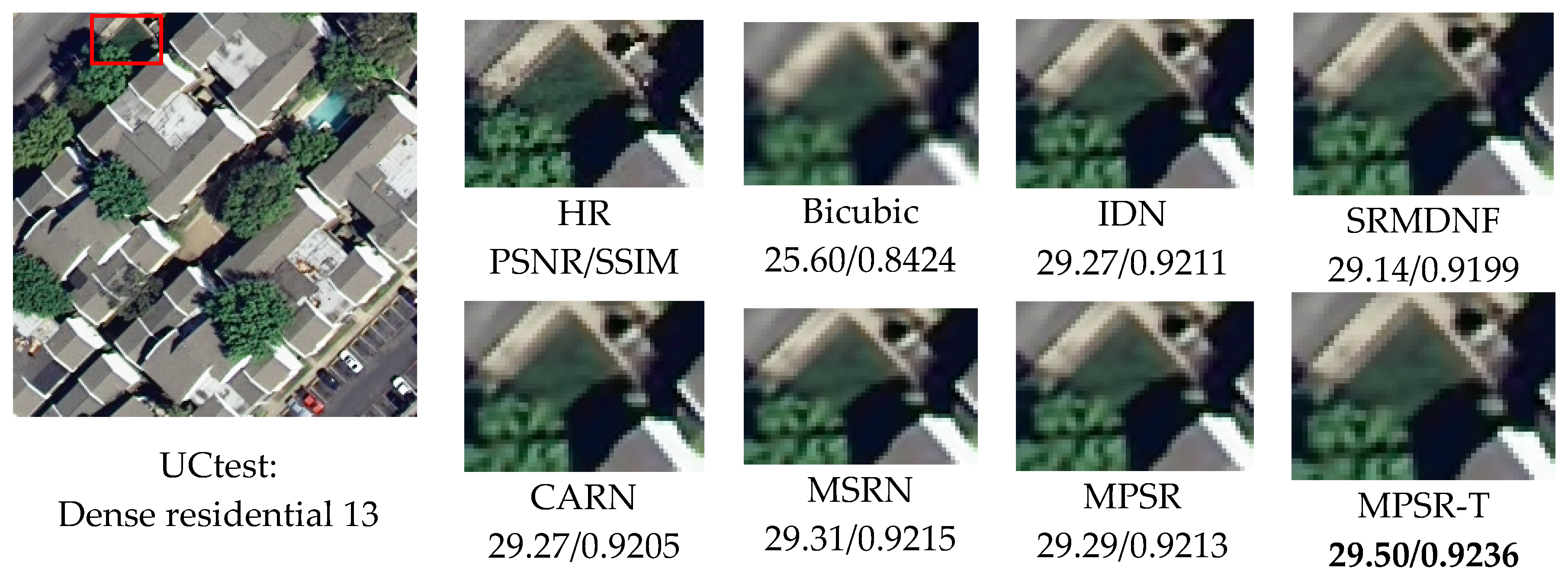
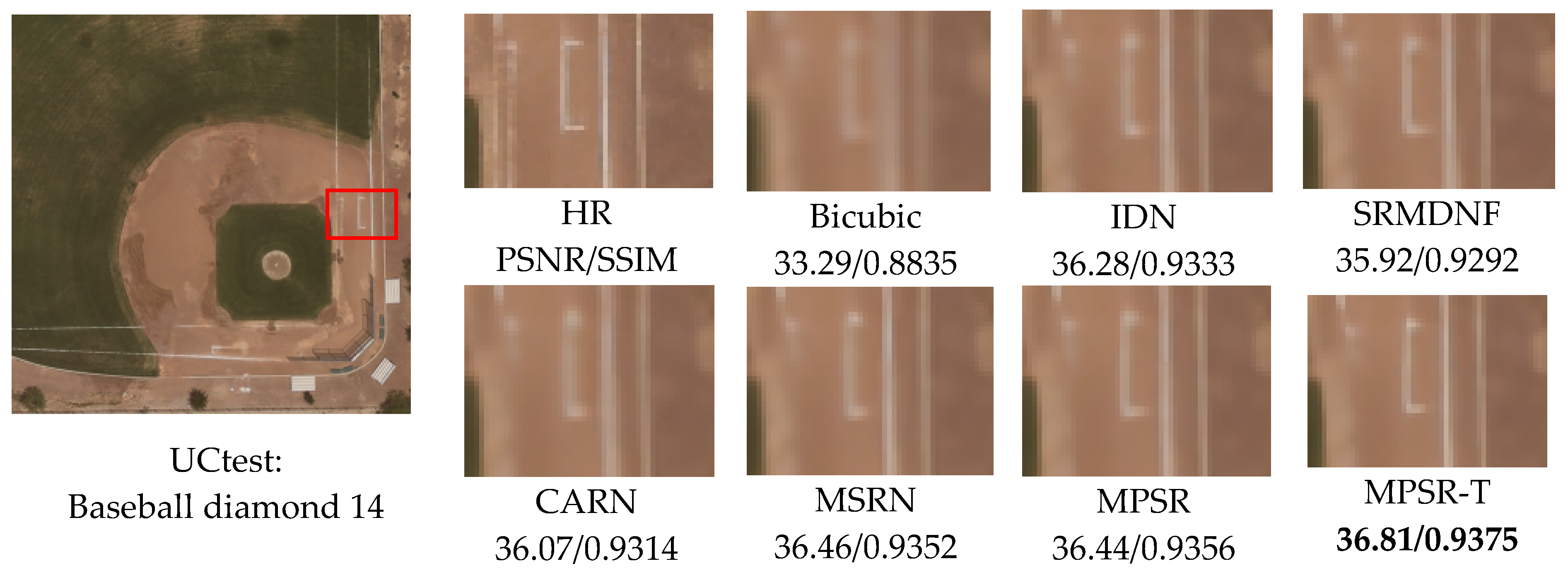
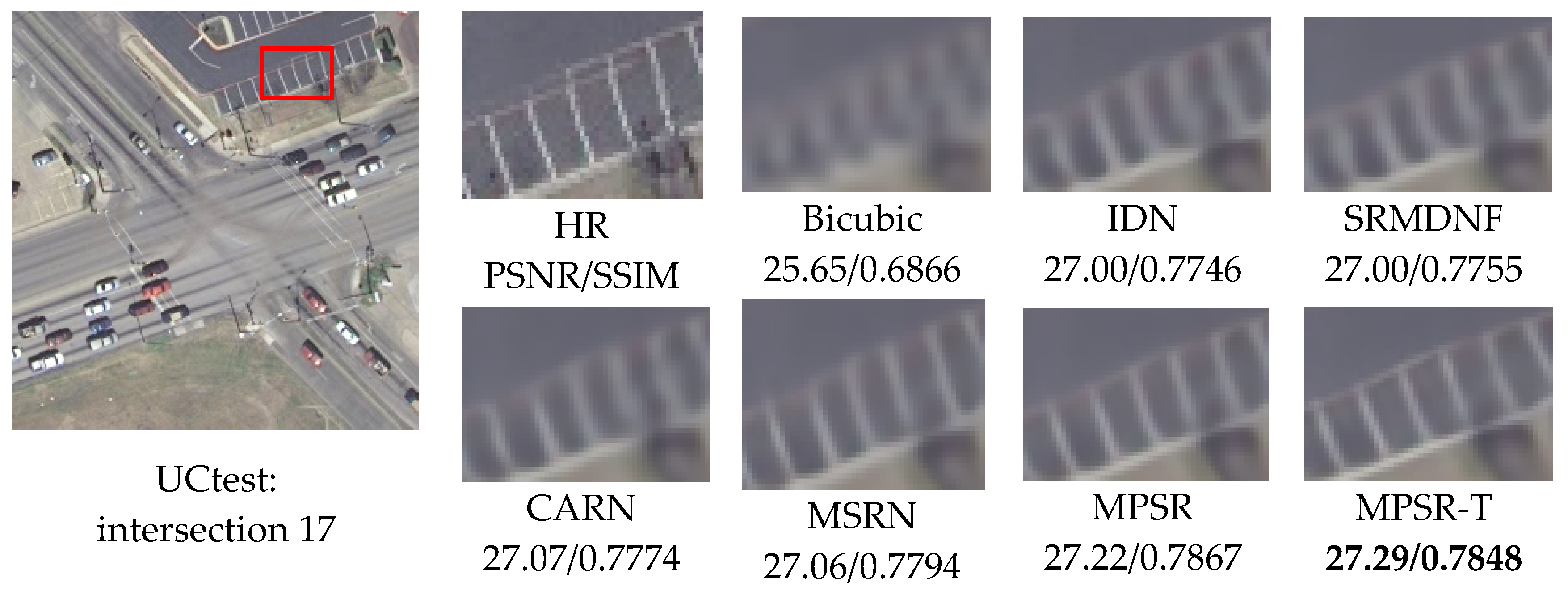
Evaluation on UCtest: MPSR and MPSR-T are adopted to super-resolve images from the UCtest. As described in Section 3.1, the UCtest is composed of 120 images randomly selected from the UC Merced land use dataset [35], which are different from transfer training samples. The reconstruction results are compared with four recent state-of-the-art methods, including IDN [16], SRMD for noise-free degradation (SRMDNF) [17], CARN [18], and MSRN [23]. All these SR algorithms were published at the world’s top computer vision conference—CVPR 2018 and ECCV 2018. Note that the MPSR is only pre-trained by the DIV2K dataset [34], a widely used SR dataset in the computer vision community. That is to say, it is fair enough to do comparisons. Also, transfer training is not performed on the state-of-the-art models.

As shown in

Table 4. UCtest ×2, ×3 and ×4 test results. Mean PSNR (the first row) and SSIM (the second row). Best results are in bold.

	Bicubic	IDN	SRMDNF	CARN	MSRN	MPSR	MPSR-T
×2	35.05	39.20	39.03	39.22	39.55	39.63	39.78
	0.9450	0.9696	0.9695	0.9695	0.9704	0.9705	0.9709
×3	29.92	33.35	32.99	33.38	33.47	33.71	33.93
	0.8627	0.9154	0.9131	0.9156	0.9163	0.9183	0.9199
×4	27.07	29.95	29.71	29.96	29.90	30.20	30.34
	0.7739	0.8528	0.8498	0.8533	0.8527	0.8571	0.8584

PSNR and SSIM represent peak signal-to-noise ratio and structural similarity index, respectively.

, the proposed MPSR and MPSR-T yield the highest scores and the second-best scores in all experiments, respectively. The gains on PSNR obtained by MPSR-T are 0.23 dB, 0.46 dB, and 0.38 dB higher than the third best approach, on the three up-sampling factors.

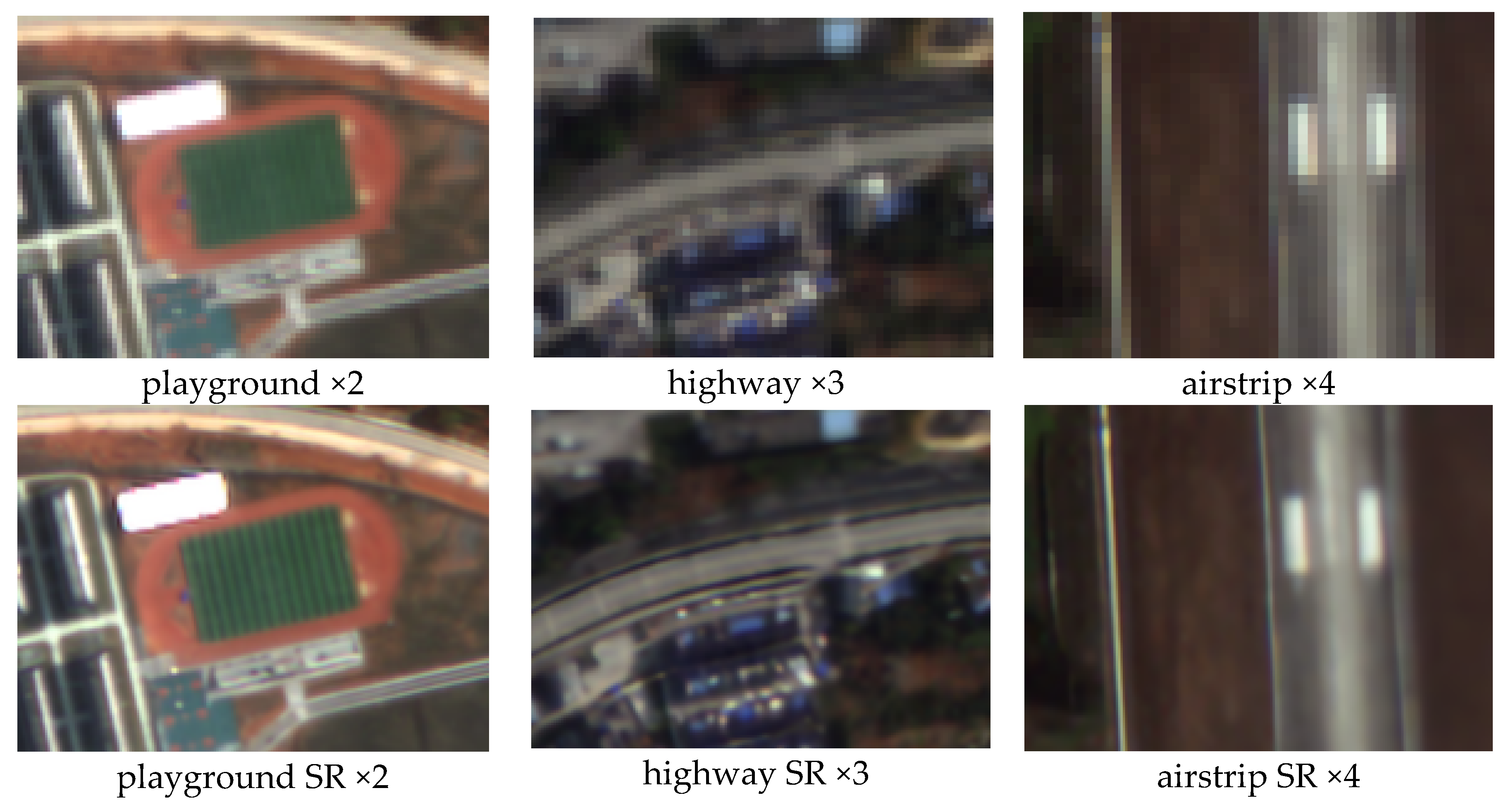
Figure 7, Figure 8, Figure 9 show the SR results with upscaling factor ×2, ×3, and ×4 of different approaches. To carry out better comparisons, some regions of original HR images and the corresponding SR reconstruction results are displayed in an enlarged scale. For example, in Figure 7, the area within the red box of the original image dense residential 13 is zoomed in by factor ×2 and named as ‘HR’. The patch named ‘Bicubic’ in the first row, which is a part of the image reconstructed by bicubic interpolation, represents the same area as patch ‘HR’. It can be seen that the left edge of the greenbelt in patch ‘MPSR-T’ is sharper than those in other reconstructed results (e.g., patch ‘MSRN’). Figure 8 shows a similar trend. As for Figure 9, the lines in some patches are blurred out while the models yield superior results.

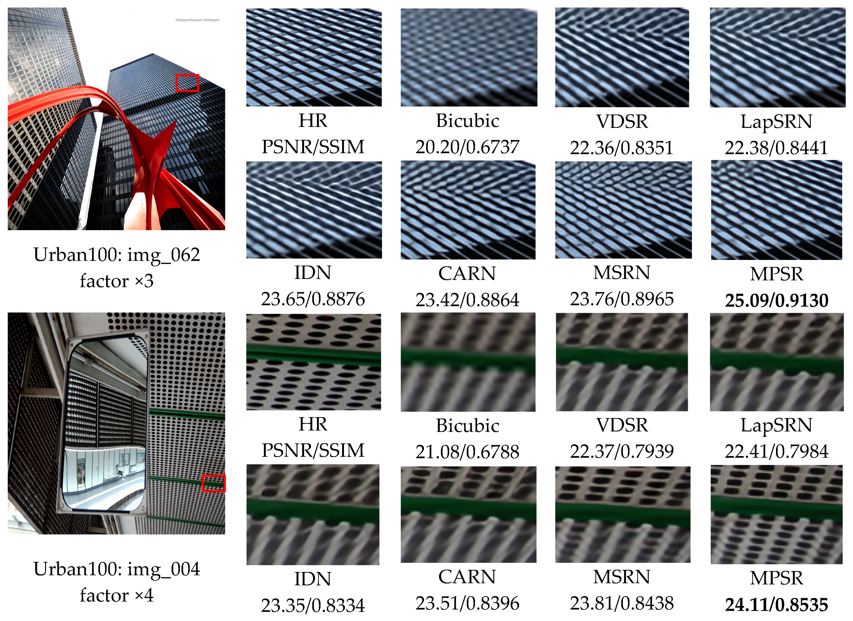
Benchmark results: To further validate the effectiveness of the proposed network, MPSR (without transfer training) is compared with 13 state-of-the-art algorithms, including SRCNN [7], VDSR [10], DRCN [11], DRRN [12], MemNet [13], LapSRN [15], IDN [16], SRMDNF [17], CARN [18], MSRN [23], SelNet [25], SRRAM [26], and SRDenseNet [30] on publicly available benchmark datasets [35,36,37,38].

In Figure 10, only two SR results of reconstructed factor ×3 and ×4 on the Urban100 dataset is provided. The difference with Figure 7, Figure 8, Figure 9 is that patches which are part of the original super-resolved images are exhibited without zooming in. As can be seen in img_062 and img_004, the five state-of-the-art methods for comparison [10,15,16,18,23] cannot clearly reconstruct the lattices and generate blurring artifacts [27]. In contrast, the MPSR can overcome the blurring artifacts better and recover image details of high fidelity and shows a significant improvement.

In a more comprehensive comparison, quantitative evaluations for reconstruction factor ×2, ×3, and ×4 on dataset Set5 [36], Set14 [37], BSD100 [38], and Urban100 [39] are provided in

Table 5. ×2, ×3, and ×4 test results on benchmark natural image sets (average PSNR and SSIM). Best results are in bold. The ‘-’ indicates the method is unsuitable to handle the images of the dataset.

Method	Set5		Set14		BSD100		Urban100
	PSNR	SSIM	PSNR	SSIM	PSNR	SSIM	PSNR	SSIM
× 2
Bicubic	33.66	0.9299	30.24	0.8688	29.56	0.8431	26.88	0.8403
SRCNN	36.66	0.9542	32.45	0.9067	31.36	0.8879	29.50	0.8946
VDSR	37.53	0.9587	33.05	0.9127	31.90	0.8960	30.77	0.9141
DRCN	37.63	0.9588	33.06	0.9121	31.85	0.8942	30.76	0.9133
DRRN	37.74	0.9591	33.23	0.9136	32.05	0.8973	31.23	0.9188
LapSRN	37.52	0.9591	33.08	0.9124	31.80	0.8949	30.41	0.9101
MemNet	37.78	0.9597	33.28	0.9142	32.08	0.8978	31.31	0.9195
IDN	37.83	0.9600	33.30	0.9148	32.08	0.8985	31.27	0.9196
SRMDNF	37.79	0.9601	33.32	0.9159	32.05	0.8985	31.33	0.9204
CARN	37.76	0.9590	33.52	0.9166	32.09	0.8978	31.92	0.9256
SelNet	37.89	0.9598	33.61	0.9160	32.08	0.8984	-	-
SRRAM	37.82	0.9592	33.48	0.9171	32.12	0.8983	32.05	0.9264
MSRN	38.08	0.9605	33.74	0.9170	32.23	0.9013	32.22	0.9326
MPSR (ours)	38.09	0.9607	33.73	0.9187	32.25	0.9005	32.49	0.9314
× 3
Bicubic	30.39	0.8682	27.55	0.7742	27.21	0.7385	24.46	0.7349
SRCNN	32.75	0.9090	29.29	0.8215	28.41	0.7863	26.24	0.7991
VDSR	33.66	0.9213	29.78	0.8318	28.83	0.7976	27.14	0.8279
DRCN	33.82	0.9226	29.77	0.8314	28.80	0.7963	27.15	0.8277
DRRN	34.03	0.9244	29.96	0.8349	28.95	0.8004	27.53	0.8377
LapSRN	33.82	0.9227	29.79	0.8320	28.82	0.7973	27.07	0.8271
MemNet	34.09	0.9248	30.00	0.8350	28.96	0.8001	27.56	0.8376
IDN	34.11	0.9253	29.99	0.8354	28.95	0.8013	27.42	0.8359
SRMDNF	34.12	0.9254	30.04	0.8382	28.97	0.8025	27.57	0.8398
CARN	34.29	0.9255	30.29	0.8407	29.06	0.8034	28.06	0.8493
SelNet	34.27	0.9257	30.30	0.8399	28.97	0.8025	-	-
SRRAM	34.30	0.9256	30.32	0.8417	29.07	0.8039	28.12	0.8507
MSRN	34.38	0.9262	30.34	0.8395	29.08	0.8041	28.08	0.8554
MPSR (ours)	34.55	0.9284	30.47	0.8450	29.18	0.8072	28.57	0.8606
× 4
Bicubic	28.43	0.8104	26.00	0.7027	25.96	0.6675	23.14	0.6577
SRCNN	30.48	0.8628	27.50	0.7513	26.90	0.7103	24.52	0.7226
VDSR	31.35	0.8838	28.02	0.7678	27.29	0.7252	25.18	0.7525
DRCN	31.53	0.8854	28.03	0.7673	27.24	0.7233	25.14	0.7511
DRRN	31.68	0.8888	28.21	0.7720	27.38	0.7284	25.44	0.7638
LapSRN	31.54	0.8866	28.19	0.7694	27.32	0.7264	25.21	0.7553
MemNet	31.74	0.8893	28.26	0.7723	27.40	0.7281	25.50	0.7630
SRDenseNet	32.02	0.8934	28.50	0.7782	27.53	0.7337	26.05	0.7819
IDN	31.82	0.8903	28.25	0.7730	27.41	0.7297	25.41	0.7632
SRMDNF	31.96	0.8925	28.35	0.7787	27.49	0.7337	25.68	0.7731
CARN	32.13	0.8937	28.60	0.7806	27.58	0.7349	26.07	0.7837
SelNet	32.00	0.8931	28.49	0.7783	27.44	0.7325	-	-
SRRAM	32.13	0.8932	28.54	0.7800	27.56	0.7350	26.05	0.7834
MSRN	32.07	0.8903	28.60	0.7751	27.52	0.7273	26.04	0.7896
MPSR (ours)	32.30	0.8968	28.74	0.7856	27.66	0.7389	26.43	0.7969

PSNR and SSIM represent peak signal-to-noise ratio and structural similarity index, respectively.

. The results of state-of-the-art methods involved are cited from their papers. It is worth pointing out that MPSR performs the best on all the benchmark natural image sets with all scaling factors. In other words, the proposed model is also a competitive candidate for super-resolving other kinds of images, not just remote sensing images.

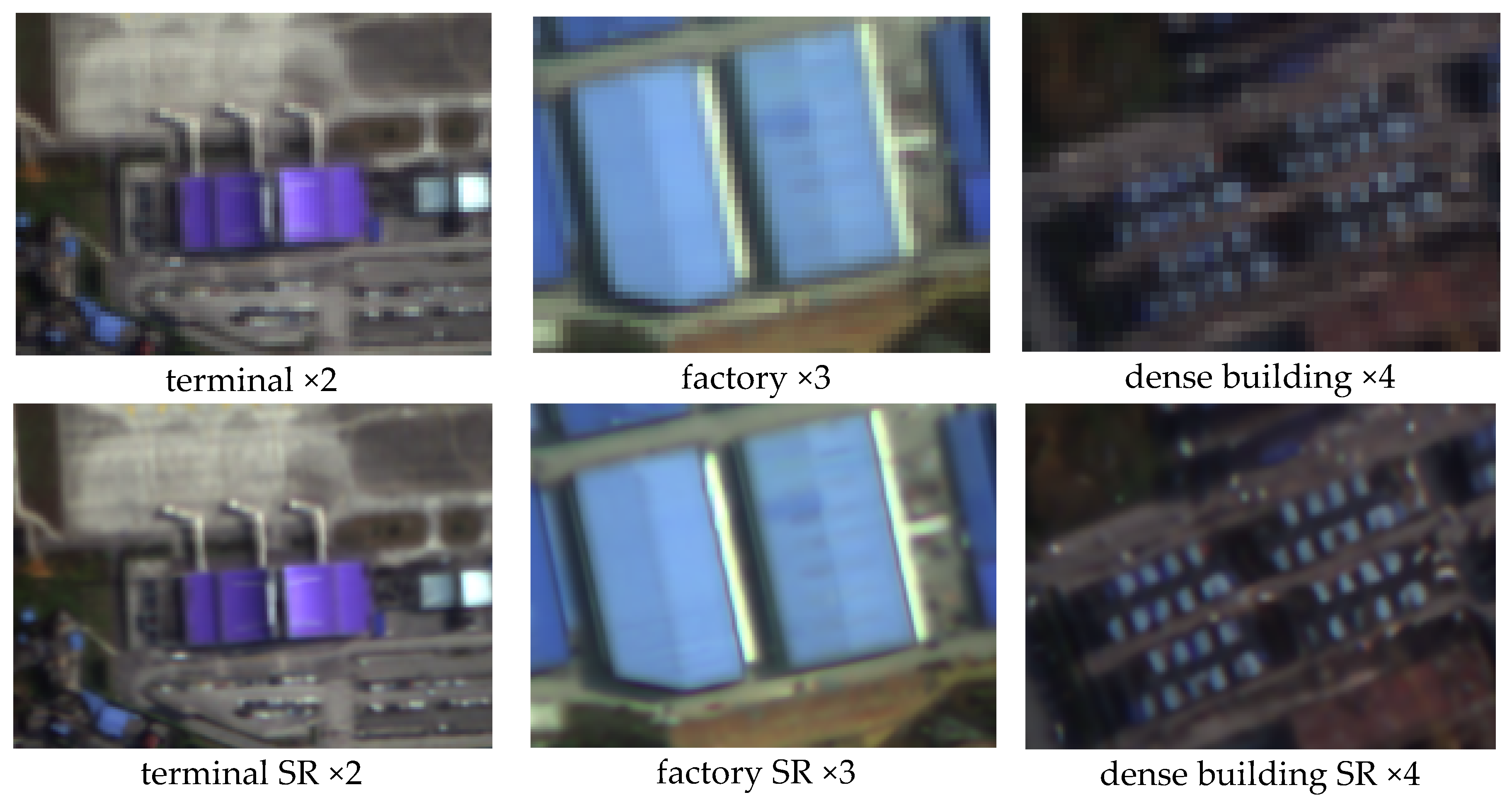
Validation by using GaoFen-1 and GaoFen-2 data: To verify the robustness of MPSR-T, some experiments are performed on multispectral remote sensing data from the GaoFen-1 satellite (medium-resolution, 8 m per pixel) and the GaoFen-2 satellite (relatively high resolution, 4 m per pixel).

Band 1, band 2, and band 3 are selected to stack into true color images before conducting the experiments, and original GaoFen-1 data and GaoFen-2 data are taken directly as LR input. Some of the test results are provided in Figure 11 and Figure 12. In Figure 11, patch ‘mountain ×2’ represents an enlarged version of the original terminal area, and ‘mountain SR ×2’ is the corresponding result of MPSR-T. It is impossible to carry out an objective evaluation with PSNR and SSIM for these reconstructed images because the real HR image is unknown. However, MPSR-T shows impressive performance when coping with remote sensing images with highly complex spatial distribution and varied-scale ground objects. For both small-scale ground features (e.g., the slight textures or edges of the playground, highway, airstrip, and mountain) and large-scale ground objects (e.g., terminal, factory, dense building, small town), satisfactory super-resolved results are obtained and the spatial resolution is significantly improved, which proved that the multi-perception network proposed achieved promising SR capacity.

4. Discussion

The methods proposed in this paper are proven to have convincing performance with extensive experimental results. In Section 3.2, the gains after adding ERBs and RCAGs clearly clarify the effectiveness of the multiple perceptual scales within the design and the rationality of treating information from different levels with unequal attentions. Then, a reasonable network structure was given by progressively modifying the number of ERBs and RCAGs, and further improving it with a transfer training strategy. In order to explore the SR capacities of the models, tests were conducted over public remote sensing data and benchmark natural image sets in Section 3.3. The results encouraged us that the models achieved pretty good performance in comparison to the world’s top SR methods and obtained satisfactory super-resolved results even when dealing with the complex and varied remote sensing images from the GaoFen-1 satellite and the GaoFen-2 satellite. From the slight lines on the playground to the indistinct but dense buildings, and so on (Figure 11), all the SR results demonstrate excellent image processing capability of the multi-perception learning-based network once again.

However, some problems were found through this research. In general, the CNN-based method could benefit from increasing the network depth, while worse test results were received when going deeper by adding ERBs (e.g., B = 9 and B = 10, see Table 2), and something similar happened when G = 4 (Table 3). This phenomenon could be related to the input images. Compared with natural images, the input images from the UC Merced dataset’s [35] lacked a high-frequency component, though they had spatial resolution of 0.3 m per pixel. Moreover, after the degradation operation before testing, the image quality gets worse. The low initial input gradients may lead to vanishing gradients during the SR process and are unsuitable for a deep network to learn or extract information. Therefore, making a good trade-off between super-resolving performance and the network setting according to the practical situation is of great importance.

In addition, an objective evaluation on super-resolved GaoFen-1 data and GaoFen-2 data could not be performed, since the real HR image is unknown. How can a more reasonable and relatively objective evaluation be performed in such case without a standard reference? It is an open issue that needs to be solved. Besides, existing CNN-based SR works mostly using a bicubic down-sampler to generate LR images. Actually, learning multiple degradations [17] or exploring real-world degradation [43] helps to train super-resolving models since the true degradation does not always follow the bicubic interpolation-based assumption. Furthermore, a high-quality dataset dedicated to remote sensing SR research is also a core issue to be solved.

5. Conclusions

In this paper, a novel multi-perception attention network (MPSR) was presented, by fully considering the complex spatial distribution of the remote sensing data and diverse spatial scales of ground objects. By incorporating the enhanced residual blocks (ERBs) and residual channel attention groups (RCAGs), MPSR achieved multi-perceptual scale learning and multi-level information adaptive weighted fusion. Also, a pre-train and transfer strategy was adopted to further improve the SR ability of the network toward remote sensing images. Extensive experimental results over remote sensing data and benchmark natural image sets demonstrated that the proposed MPSR achieves superior performance compared to the state-of-the-art methods. It is worth mentioning that MPSR is also a competitive candidate for super-resolving other kinds of images.

6. Patents

The patent 201911140450.X results from the work reported in this manuscript.

References

- Beaulieu, M.; Foucher, S.; Haberman, D.; Stewart, C. Deep image-to-image transfer applied to resolution enhancement of Sentinel-2 images. In Proceedings of the IEEE International Geoscience and Remote Sensing Symposium, Valencia, Spain, 22–27 July 2018; pp. 2611–2614. [Google Scholar]
- Huang, N.; Yang, Y.; Liu, J.; Gu, X.; Cai, H. Single-image super-resolution for remote sensing data using deep residual-learning neural network. In Proceedings of the International Conference on Neural Information Processing, Guangzhou, China, 14–18 November 2017. [Google Scholar]
- Liebel, L.; Körner, M. Single-image super resolution for multispectral remote sensing data using convolutional neural networks. In Proceedings of the International Archives of the Photogrammetry, Remote Sensing and Spatial Information Sciences, Prague, Czech Republic, 12–19 July 2016. [Google Scholar]
- Li, F.; Xin, L.; Guo, Y.; Gao, D.; Kong, X.; Jia, X. Super-resolution for GaoFen-4 remote sensing images. IEEE Geosci. Remote Sens. Lett. 2018, 15, 28–32. [Google Scholar] [CrossRef]
- Li, F.; Xin, L.; Guo, Y.; Gao, J.; Jia, X. A framework of mixed sparse representations for remote sensing images. IEEE Trans. Geosci. Remote Sens. 2017, 55, 1210–1221. [Google Scholar] [CrossRef]
- Yuan, Q.; Zhang, L.; Shen, H. Multiframe super-resolution employing a spatially weighted total variation model. IEEE Trans. Circuits Syst. Video Technol. 2012, 22, 379–392. [Google Scholar] [CrossRef]
- Dong, C.; Loy, C.C.; He, K.; Tang, X. Image super-resolution using deep convolutional networks. IEEE Trans. Pattern Anal. Mach. Intell. 2016, 38, 295–307. [Google Scholar] [CrossRef] [PubMed]
- Shi, W.; Caballero, J.; Huszár, F.; Totz, J.; Aitken, A.P.; Bishop, R.; Rueckert, D.; Wang, Z. Real-time single image and video super-resolution using an efficient sub-pixel convolutional neural network. In Proceedings of the IEEE Conference on Computer Vision and Pattern Recognition, Las Vegas, NV, USA, 27–30 June 2016; pp. 1874–1883. [Google Scholar]
- He, K.; Zhang, X.; Ren, S.; Sun, J. Deep residual learning for image recognition. In Proceedings of the IEEE Conference on Computer Vision and Pattern Recognition, Las Vegas, NV, USA, 27–30 June 2016; pp. 770–778. [Google Scholar]
- Kim, J.; Lee, J.K.; Lee, K.M. Accurate image super-resolution using very deep convolutional networks. In Proceedings of the IEEE Conference on Computer Vision and Pattern Recognition, Las Vegas, NV, USA, 27–30 June 2016; pp. 1646–1654. [Google Scholar]
- Kim, J.; Lee, J.K.; Lee, K.M. Deeply-recursive convolutional network for image super-resolution. In Proceedings of the IEEE Conference on Computer Vision and Pattern Recognition, Las Vegas, NV, USA, 27–30 June 2016; pp. 1637–1645. [Google Scholar]
- Tai, Y.; Yang, J.; Liu, X. Image super-resolution via deep recursive residual network. In Proceedings of the IEEE Conference on Computer Vision and Pattern Recognition, Honolulu, HI, USA, 21–26 July 2017; pp. 2790–2798. [Google Scholar]
- Tai, Y.; Yang, J.; Liu, X.; Xu, C. MemNet: A Persistent Memory Network for Image Restoration. In Proceedings of the IEEE International Conference on Computer Vision, Venice, Italy, 22–29 October 2017; pp. 4549–4557. [Google Scholar]
- Ledig, C.; Theis, L.; Huszar, F.; Caballero, J.; Cunningham, A.; Acosta, A.; Aitken, A.; Tejani, A.; Totz, J.; Wang, Z.; et al. Photo-realistic single image super-resolution using a generative adversarial network. In Proceedings of the IEEE Conference on Computer Vision and Pattern Recognition, Honolulu, HI, USA, 21–26 July 2017; pp. 105–114. [Google Scholar]
- Lai, W.S.; Huang, J.B.; Ahuja, N.; Yang, M.H. Deep laplacian pyramid networks for fast and accurate super-resolution. In Proceedings of the IEEE Conference on Computer Vision and Pattern Recognition, Honolulu, HI, USA, 21–26 July 2017; pp. 5835–5843. [Google Scholar]
- Hui, Z.; Wang, X.; Gao, X. Fast and accurate single image super-resolution via information distillation network. In Proceedings of the IEEE Conference on Computer Vision and Pattern Recognition, Salt Lake City, UT, USA, 18–22 June 2018; pp. 723–731. [Google Scholar]
- Zhang, K.; Zuo, W.; Zhang, L. Learning a single convolutional super-resolution network for multiple degradations. In Proceedings of the IEEE Conference on Computer Vision and Pattern Recognition, Salt Lake City, UT, USA, 18–22 June 2018; pp. 3262–3271. [Google Scholar]
- Ahn, N.; Kang, B.; Sohn, K.A. Fast, accurate, and lightweight super-resolution with cascading residual network. In Proceedings of the European Conference on Computer Vision, Munich, Germany, 8–14 September 2018. [Google Scholar]
- Luo, Y.; Zhou, L.; Wang, S.; Wang, Z. Video satellite imagery super resolution via convolutional neural networks. IEEE Geosci. Remote Sens. Lett. 2017, 14, 2398–2402. [Google Scholar] [CrossRef]
- Lei, S.; Shi, Z.; Zou, Z. Super-resolution for remote sensing images via local–global combined network. IEEE Geosci. Remote Sens. Lett. 2017, 14, 1243–1247. [Google Scholar] [CrossRef]
- Xu, W.; Xu, G.; Wang, Y.; Sun, X.; Lin, D.; Wu, Y. High quality remote sensing image super-resolution using deep memory connected network. In Proceedings of the IEEE International Geoscience and Remote Sensing Symposium, Valencia, Spain, 22–27 July 2018; pp. 8889–8892. [Google Scholar]
- Mario, H.J.; Ruben, F.B.; Paoletti, M.E.; Javier, P.; Antonio, P.; Filiberto, P. A new deep generative network for unsupervised remote sensing single-image super-resolution. IEEE Trans. Geosci. Remote Sens. 2018, 56, 6792–6810. [Google Scholar]
- Li, J.; Fang, F.; Mei, K.; Zhang, G. Multi-scale residual network for image super-resolution. In Proceedings of the European Conference on Computer Vision, Munich, Germany, 8–14 September 2018; pp. 527–542. [Google Scholar]
- Hu, J.; Shen, L.; Albanie, S.; Sun, G.; Wu, E. Squeeze-and-excitation networks. In Proceedings of the IEEE Conference on Computer Vision and Pattern Recognition, Salt Lake City, UT, USA, 18–22 June 2018; pp. 7132–7141. [Google Scholar]
- Choi, J.S.; Kim, M. A deep convolutional neural network with selection units for super-resolution. In Proceedings of the IEEE Conference on Computer Vision and Pattern Recognition Workshops, Honolulu, HI, USA, 21–26 July 2017; pp. 1150–1156. [Google Scholar]
- Kim, J.H.; Choi, J.H.; Cheon, M.; Lee, J.S. Ram: Residual attention module for single image super-resolution. arXiv 2018, arXiv:1811.12043. [Google Scholar]
- Zhang, Y.; Li, K.; Li, K.; Wang, L.; Zhong, B.; Fu, Y. Image super-resolution using very deep residual channel attention networks. In Proceedings of the European Conference on Computer Vision, Munich, Germany, 8–14 September 2018; pp. 286–301. [Google Scholar]
- Zhao, H.; Gallo, O.; Frosio, I.; Kautz, J. Loss functions for image restoration with neural networks. IEEE Trans. Comput. Imaging 2017, 3, 47–57. [Google Scholar] [CrossRef]
- Lim, B.; Son, S.; Kim, H.; Nah, S.; Lee, K.M. Enhanced deep residual networks for single image super-resolution. In Proceedings of the IEEE Conference on Computer Vision and Pattern Recognition Workshops, Honolulu, HI, USA, 21–26 July 2017; pp. 1132–1140. [Google Scholar]
- Tong, T.; Li, G.; Liu, X.; Gao, Q. Image super-resolution using dense skip connections. In Proceedings of the IEEE International Conference on Computer Vision, Venice, Italy, 22–29 October 2017; pp. 4809–4817. [Google Scholar]
- Nair, V.; Hinton, G.E. Rectified linear units improve restricted Boltzmann machines. In Proceedings of the 27th International Conference on Machine Learning, Haifa, Israel, 21–25 June 2010. [Google Scholar]
- Dong, C.; Loy, C.C.; Tang, X. Accelerating the super-resolution convolutional neural network. In Proceedings of the European Conference on Computer Vision, Berlin, Germany, 27–30 June 2016; pp. 391–407. [Google Scholar]
- Pan, S.J.; Qiang, Y. A survey on transfer learning. IEEE Trans. Knowl. Data Eng. 2010, 22, 1345–1359. [Google Scholar] [CrossRef]
- Timofte, R.; Lee, K.M.; Wang, X.; Tian, Y.; Ke, Y.; Zhang, Y.; Wu, S.; Dong, C.; Lin, L.; Qiao, Y.; et al. NTIRE 2017 challenge on single image super-resolution: Methods and results. In Proceedings of the IEEE Conference on Computer Vision and Pattern Recognition Workshops, Honolulu, HI, USA, 21–26 July 2017; pp. 1110–1121. [Google Scholar]
- Yang, Y.; Newsam, S. Bag-of-visual-words and spatial extensions for land-use classifification. In Proceedings of the 18th SIGSPATIAL International Conference On Advances in Geographic Information Systems, Seattle, WA, USA, 2–5 November 2010; pp. 270–279. [Google Scholar]
- Bevilacqua, M.; Roumy, A.; Guillemot, C.; Morel, M.L.A. Low-complexity single-image super-resolution based on nonnegative neighbor embedding. In Proceedings of the British Machine Vision Conference, Guildford, UK, 3–7 September 2012. [Google Scholar]
- Zeyde, R.; Elad, M.; Protter, M. On single image scale-up using sparse-representations. In Proceeding of the 7th International Conference on Curves and Surfaces, Avignon, France, 24–30 June 2010. [Google Scholar]
- Martin, D.; Fowlkes, C.; Tal, D.; Malik, J. A database of human segmented natural images and its application to evaluating segmentation algorithms and measuring ecological statistics. In Proceedings of the 8th IEEE International Conference on Computer Vision, Vancouver, BC, Canada, 7–14 July 2001. [Google Scholar]
- Huang, J.B.; Singh, A.; Ahuja, N. Single image super-resolution from transformed self-exemplars. In Proceedings of the IEEE Conference on Computer Vision and Pattern Recognition, Boston, MA, USA, 8–10 June 2015; pp. 5197–5206. [Google Scholar]
- Kingma, D.P.; Ba, J. Adam: A method for stochastic optimization. In Proceedings of the 3rd International Conference for Learning Representations, San Diego, CA, USA, 7–9 May 2015. [Google Scholar]
- Paszke, A.; Gross, S.; Chintala, S.; Chanan, G.; Yang, E.; DeVito, Z.; Lin, Z.; Desmaison, A.; Antiga, L.; Lerer, A. Automatic differentiation in pytorch. In Proceedings of the 31st Conference on Neural Information Processing Systems, Long Beach, CA, USA, 4–9 December 2017. [Google Scholar]
- Wang, Z.; Bovik, A.C.; Sheikh, H.R.; Simoncelli, E.P. Image quality assessment: From error visibility to structural similarity. IEEE Trans. Image Process. 2004, 13, 600–612. [Google Scholar] [CrossRef] [PubMed] [Green Version]
- Bulat, A.; Yang, J.; Tzimiropoulos, G. To learn image super-resolution, use a gan to learn how to do image degradation first. In Proceedings of the European Conference on Computer Vision, Munich, Germany, 8–14 September 2018; pp. 185–200. [Google Scholar]
Figure 1.
Multi-perception attention network (MPSR).
Figure 2.
Comparison of residual blocks: (a) the residual block in SRResNet, (b) common residual block structure (RB), and (c) proposed enhanced residual block (ERB).
Figure 3.
Residual channel attention group (RCAG).
Figure 4.
Channel attention (CA). represents the element-wise product.
Figure 5.
Representative images from the datasets used for comparing and evaluating algorithms. (a) DIV2K, (b) UC MERCED, (c) Set5, (d) Set14, (e) BSD100, (f) Urban100.
Figure 6.
Effect of using the pre-training strategy. (a) Performance of training ×3 MPSR by using the pre-trained ×2 model. (b) Performance of training ×3 MPSR from scratch. Image 0801 to 0805 from the DIV2K dataset are used for validation during training.
Figure 7.
Visual comparison of ×2 SR results of the UCtest. The best results are in bold.
Figure 8.
Visual comparison of ×3 SR results of the UCtest. The best results are in bold.
Figure 9.
Visual comparison of ×4 SR results of the UCtest. The best results are in bold.
Figure 10.
Visual comparisons of Urban100. The best results are in bold.
Figure 11.
×2, ×3, and ×4 SR results of the GaoFen-1 data.
Figure 12.
×2, ×3, and ×4 SR results of the GaoFen-2 data.