Synergy of Satellite Remote Sensing and Numerical Ocean Modelling for Coastal Geomorphology Diagnosis

Abstract

Sediment dynamics is the primary driver of the evolution of the coastal geomorphology and of the underwater shelf clinoforms. In this paper, we focus on mesoscale and sub-mesoscale processes, such as coastal currents and river plumes, and how they shape the sediment dynamics at regional or basin spatial scales. A new methodology is developed that combines observational data with numerical modelling: the aim is to pair satellite measurements of suspended sediment with velocity fields from numerical oceanographic models, to obtain an estimation of the sediment flux. A numerical divergence of this flux is then computed. The divergence field thus obtained shows how the aforementioned mesoscale processes distribute the sediments. The approach was applied and discussed on the Adriatic Sea, for the winter of 2012, using data provided by the ESA Coastcolour project and the output of a run of the MIT General Circulation Model.

1. Introduction

The morphological evolution of shoreline, coastal features, lagoons, deltas and clinoforms on continental shelves, in absence of relative sea level changes, due to either eustacy or local tectonism, is primarily driven by the sediment dynamics and the sediment transport [1,2,3,4,5]. Seminal studies, indeed, highlight the role of coastal plumes or river runoff, and their sediment loads, in contributing to sediment availability for coastal and continental shelf morphodynamics [5,6].

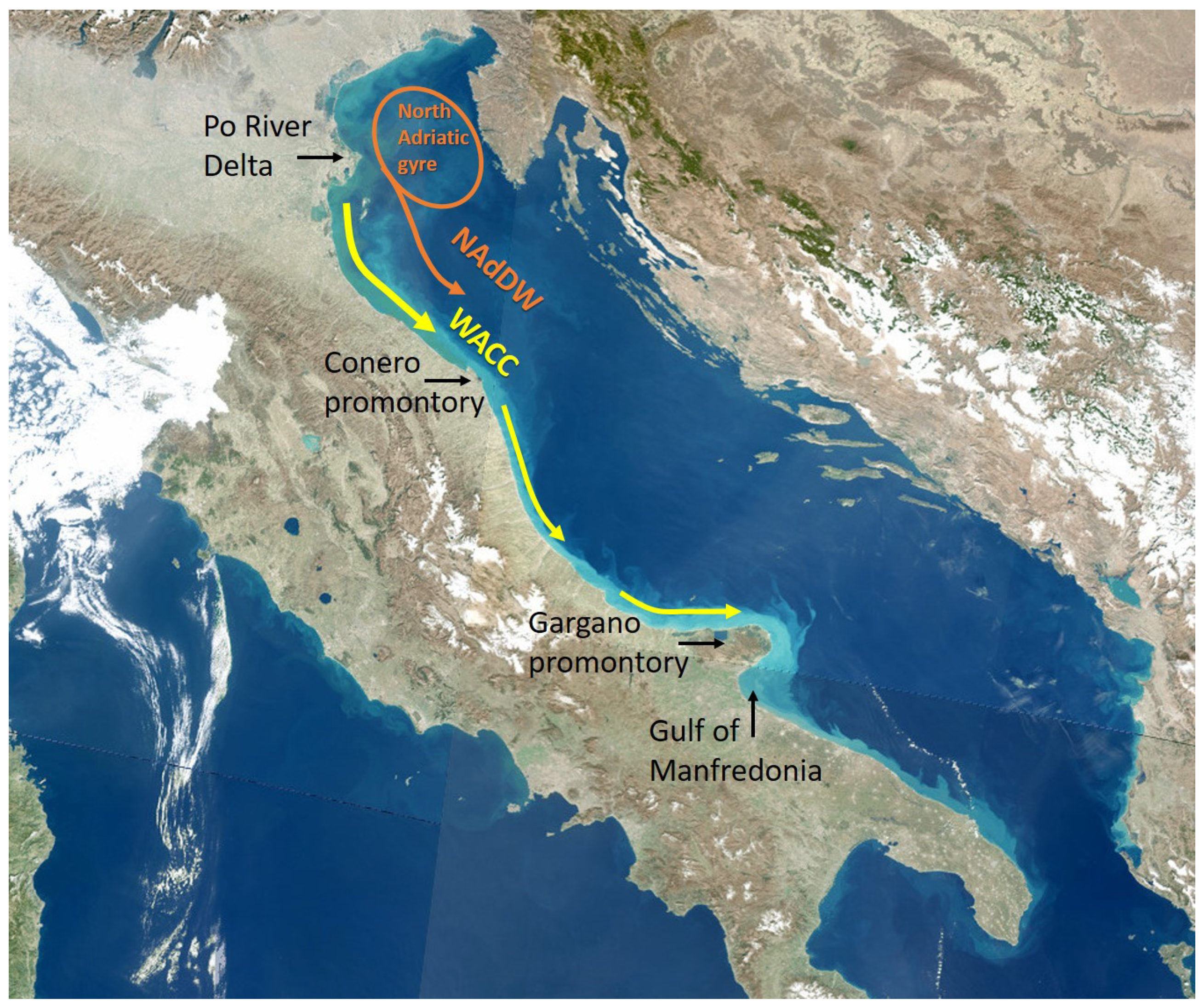
In particular, in the Adriatic sub-basin (Mediterranean Sea; Figure 1), Bignami et al. [7] investigated the variability of the Western Adriatic Coastal Current (WACC), and its turbid, Case 2 waters, in relation to circulation patterns and to wind regimes. Brando et al. [8] investigated river plumes at mesoscale and submesoscale in the North Adriatic Sea (NAS), by means of coupled satellite data and numerical modelling. On the other hand, Cattaneo et al. [9] and Sherwood et al. [10] focused on the sediment erosion, transport and deposition in the Adriatic Sea. The Adriatic Sea, especially its western side, the Italian east coast, is a case study for this kind of phenomena, because of its characteristic coastal flow dynamics and the significant role of river sediment inputs on the northwest side of the basin [7,9,10,11].

Indeed, the circulatory regime of this basin, as described in [12], is dominated by:

• a cyclonic gyre with a component that flows parallel to the western shoreline (Figure 1), mainly generated by the wind patterns;
• the North Adriatic Dense Water (NAdDW; Figure 1) that forms in the northern Adriatic through winter cooling and then, once a density threshold is reached, flows southward until cascading toward the deep southern Adriatic Basin; and
• the Levantine Intermediate Water (LIW), a salty water that forms in the Eastern Mediterranean Sea and intrudes in the Adriatic basin flowing at depths of 200–600 m.

An intensified western boundary current, the Western Adriatic Coastal Current (WACC), flows southward with long-term average speeds that reach 0.20 m s${}^{-1}$ at some locations [13]. The overall thermohaline circulation runs along the Italian coast, constraining the main sediment flux to deposit in a prism parallel to the coast. The investigation of sediment dynamics along the coastal Adriatic currents, besides the use of in-situ measurements and numerical modelling, is largely improved by remote sensing observations and analyses [4,14,15].

Figure 1 shows a combination of the views acquired on 28 February 2019 by the OLCI sensors on board of the Sentinel-3A and Sentinel-3B spacecrafts. In this true colour picture the Western Adriatic Coastal Current (WACC) is clearly visible, by means of its suspended sediment load, which is transported along the coast. The sediment laden plume originates from river inputs at the northwest sector of the sub-basin [8] and receives the contribution of other small rivers in the central part. Sediment dynamics does not reduce to the settling of the sediment suspended in the coastal plume [16]. Longshore sediment transport in the littoral and coastal plume systems are the main cause of the sediment load distribution along the coast, without, or with a limited, net sediment offshore export. The redistribution of the sediment load over the entire inner shelf is instead caused by the action of meteorological events, varying currents and wind waves, which resuspend and transport sediments in deeper water.

The link between the sediment dynamics and the most general model for morphodynamics is provided by the Exner equation. Exner [17,18] proposed that the change in time of the local elevation $\eta (x,t)$ of the bed of a river or channel is proportional to the spatial rate of change of the average flow velocity:

$$\frac{\partial \eta }{\partial t}=-A\frac{\partial v}{\partial x}$$

(1)

In the text describing the equation, Exner explained that he intended the flow velocity v as a proxy for the sediment flux [19].

Thus, the Exner equation, in its general formulation, is now written as a classical conservation law:

$$\frac{\partial \eta }{\partial t}=-\frac{1}{{ϵ}_0}\nabla ·{\overrightarrow{q}}_s$$

(2)

that relates the seabed elevation ($\eta$), relative to a fixed datum, with the sediment that is transported by water (${\overrightarrow{q}}_s$ is the sediment flux). The bed elevation increases ($\frac{\partial \eta }{\partial t}>0$) proportionally to the sediment that is dropping out of the transport (negative sediment flux divergence, $\nabla ·{\overrightarrow{q}}_s<0$). Conversely, the bed elevation decreases proportionally to the sediment that becomes entrained by the flow (positive sediment flux divergence, $\nabla ·{\overrightarrow{q}}_s>0$). The proportionality factor is the inverse of the grain packing density, ${ϵ}_0$.

Paola and Voller [19] provided a complete generalisation of the Exner equation to address several different processes over a wide array of temporal scales.

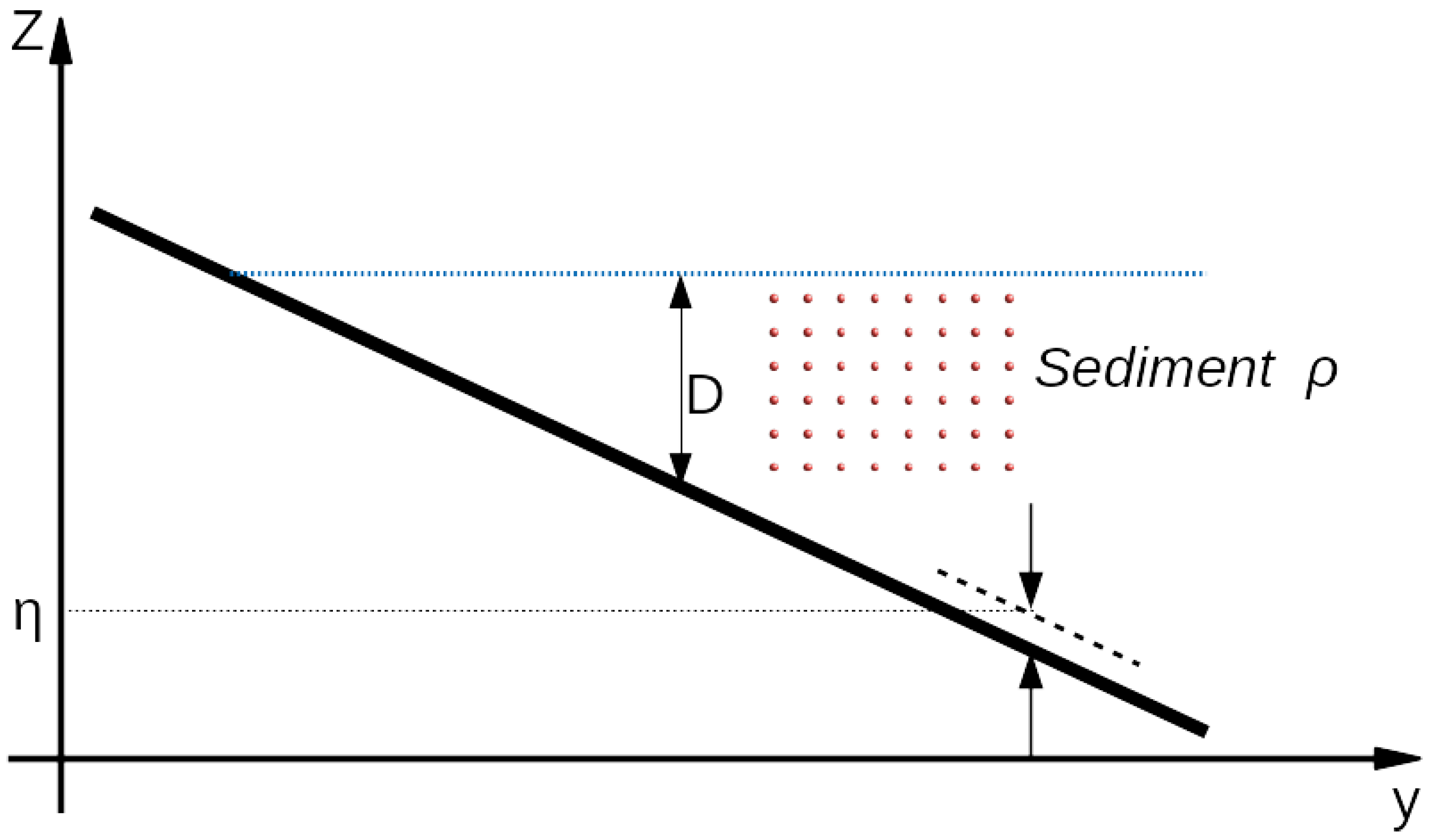
Equation (2) can be related to coastal geomorphology and, in particular, to sediment availability along the inner shelf, since a positive divergence of sediment flux suggests sediment erosion, while a negative divergence suggests sediment deposition. Figure 2 sketches a simplified geometry that can be adopted to represent the seabed near the shoreline. The x-axis is usually taken parallel to the shoreline itself, and it is possibly a curvilinear coordinate, while the y-axis is usually taken seaward, orthogonal to the shoreline. The z-axis is usually the vertical, with the positive direction pointing up and the zero value at the sea surface. The seabed height $\eta$ is clearly indicated. $\rho$ represents the sediment concentration in the water.

The practical application of the Exener equation (Equation (2)) relies on a proper estimation of the sediment flux ${\overrightarrow{q}}_s$. At local scale, sediment dynamics is primarily dominated by waves and wave-induced currents, especially during strong meteorological events. Several empirical or semi-empirical relations have been proposed to correlate the sediment flux to the wave field parameters and to the sediment grain size [20,21,22,23]. All these approaches, however, when considering time scales longer than the single meteorological event, lead to considering only a prevalent wave field, or a small set of prevalent wave fields that could happen in the time frame under investigation. While they are able to produce good estimations of erosion vs. deposition in local spatial and temporal scales, or to stable vs. unstable shoreline profiles, they are usually not applied to wider scales.

The scope of our work, instead, is to investigate the sediment dynamics at larger spatial and temporal scales, by analysing coastal sediment plumes and coastal currents with a synergic approach, combining observational data with numerical modelling. Marine coastal currents are strongly influenced by the input of fresh waters, tides, topographic features and winds. Moreover, hydrodynamics typically observed in coastal areas involves processes interacting on a wide range of spatial and temporal scales. In our work, we make use of a suitable numerical run that is able to capture the coastal processes, such as buoyant plume formation and propagation, as well as associated coastal upwelling and downwelling [24].

We envisage the need to move from an empirical to an observational approach, and thus we look for alternative estimations of the sediment flux. As a general statement, the flux of sediment in the water, can be expressed in terms of the suspended sediment concentration in the water $\rho$ and the water velocity $\overrightarrow{u}$:

$${\overrightarrow{q}}_{3D}=\rho \overrightarrow{u}$$

(3)

As better explained in Section 2, optical observations are able to estimate physical, chemical and biological properties of the water. IOPs (Inherent Optical Properties), AOPs (Apparent Optical Properties) and water constituents can be retrieved by means of proven algorithms from remote sensing observations in the visible and in the near-infrared spectrum. The concentration of suspended matter is one the water constituent that can be retrieved from such observations [25,26,27]. Spaceborne sensors are one of the most important sources of optical observations, due to their great temporal and spatial coverage.

It is then natural to plug the remotely-sensed TSM (Total Suspended Matter) as the sediment concentration $\rho$ in Equation (3). In the same way, a water velocity field derived from an oceanographic model can be plugged as the velocity $\overrightarrow{u}$ in Equation (3).

2. Materials and Methods

To show the feasibility of our approach, we need to combine a remotely sensed sediment concentration field with a velocity field from an oceanographic model to obtain a sediment flux to feed in the Exner equation (Equation (2)) and thus estimate the sediment erosion and deposition processes (i.e., the temporal evolution of the seabed height $\eta$). The data sources we chose for our first experiments are:

• for the TSM fields, the ESA Coastcolour project [28]; and
• for the velocity field, a MITgcm (Massachusetts Institute of Technology General Circulation Model [29])-based model for the Adriatic Sea, run by ENEA-ISMAR

The reasons for such a choice were the quality and the ready availability of these two datasets. As better explained in the following paragraphs, these two datasets overlap for a small time window. Actually the model availability time frame (just four months) almost entirely lies within the ESA Coastcolour project time frame (nine years).

2.1. Remote Sensing Data

The Coastcolour project [28], launched by ESA to fully exploit the potential of the MERIS instrument, provides us a complete (from 4 January 2003 to 7 April 2012, when the mission ended) series of ocean optics observation of a set of basins where the presence of Case 2, optically complex waters is important. The whole Mediterranean, and thus the Adriatic Sea, is among these basins. The Coastcolour project provides three levels of products:

• The Level 1P product (L1P) provides top of atmosphere radiance, with geolocation, equalisation to reduce coherent noise, smile correction, pixel characterisation information (cloud, snow, etc.) and a precise coastline.
• The Level 2R (L2R) product is the result of a neural network based atmospheric correction, which is applicable for a large range of water type, from clear to extreme scattering waters; it contains water leaving reflectance, normalised water leaving reflectance and different information about atmospheric properties.
• The Level 2W (L2W) product provides information about water properties such as IOPs (Inherent Optical Properties) and water constituent concentrations.

Among the water constituent concentrations provided by L2W product, there is the concentration of the Total Suspended Matter variable (conc_tsm) that we use as an estimation of the sediment concentration in water, $\rho$. As per the “Validation Report” from the “Publication” section of the Coastcolour website [28], the correlation coefficient and the coefficient of determination ($R^2$) of the (conc_tsm) versus the in-situ validation dataset ([30]) are, respectively, 0.831 and 0.691. Refer to the “Publication” section of the Coastcolour website [28] for the complete documentation on the algorithms and on the validation processes that have been used to create and validate all the Coastcolour products.

2.2. Numerical Model Outputs

In this work we make use of a MITgcm run that has been setup to investigate coastal upwelling and downwelling processes in the Adriatic Sea during a strong dense water event that occurred in winter 2012 [24]. The model domain, which covers the entire Adriatic Sea, is discretised by a non-uniform curvilinear orthogonal grid of 432 × 1296 points, with 100 vertical levels. This grid has a variable resolution, ranging from less than 500 m in the nearshore area up to 1000–2000 m offshore. Furthermore, it is orthogonal, or almost orthogonal, to most of the coastline. Regarding the vertical resolution, the grid has 100 vertical z levels with a thickness of 1 m in the upper 23 m gradually increasing to a maximum of 17 m for the remaining 64 levels.

The model simulations started at the beginning of December 2011 and finished at the end of April 2012. Simulated fields and diagnostic were produced every three simulated hours. The bathymetry used by MITgcm is provided by the National Group of Operational Oceanography (GNOO; http://gnoo.bo.ingv.it/bathymetry/). As in [31,32], an implicit linear formulation of the free surface is used. The river runoff was considered explicitly and modelled as a lateral open-boundary condition. Rivers were included by introducing small channels in the bathymetry that simulate the river bed close to the coast. Velocity was imposed at the upstream end of each channel, with the prescribed discharge rate being obtained by multiplying the velocity by the cross sectional area of the channel. No flux conditions for either momentum or tracers and no slip conditions for momentum were imposed at the solid boundaries. Bottom drag was expressed as a quadratic function of the mean flow in the bottom layer. The net transport through the southern open boundary was corrected during run-time at each time step to balance the effects of river discharge and of the evaporation minus precipitation budget on the surface level. This solution prevented any unrealistic drift in the sea surface elevation. Tides were imposed as a barotropic velocity at the southern boundary. At the surface, the wind drag coefficient was computed following the default MITgcm formulation:

$$C_d=\frac{0.0027}{U_{10}}+0.000142+0.0000764·U_{10}$$

(4)

where $U_{10}$ is the wind speed at 10 m. The wind speed and direction, together with the other surface forcings (air temperature, relative humidity, and cloud cover), were provided by means of hourly meteorological forecasts from the MOLOCH (MOdello LOCale in H coordinates) model, developed and run at the ISAC (Institute of Atmospheric Sciences and Climate—National Research Council) CNR, Bologna, Italy [33,34,35]. The numerical run was finally validated by using time series of surface and bottom temperature as well as surface salinity from the VIDA buoy [24]. Refer to McKiver et al. [24] for the full description of the model set-up, the experiments and their validation. The model has been geared to investigate coastal processes, and the MITgcm capabilities in capturing them. This feature and its horizontal resolution that, near the shore, is comparable with the Coastcolour TSM field, are the key advantage of this model in our study. Other models and other velocity fields (e.g., from reanalysis products) we tested did not provide meaningful divergence fields. Hereafter, we call Winter2012 this model run as well as its grid.

2.3. Combining Marine Currents and TSM Upstream Data

As aforesaid, these two datasets (i.e., Coastcolour TSM satellite product and the Winter2012 MITgcm run for marine currents) overlap for only a four-month time window; however we considered this sufficient to test our approach. The TSM concentration field $\rho$ from the satellite data is inherently bidimensional, while the velocity field $\overrightarrow{u}$ from the model is tridimensional. We have to consider this aspect when formulating our sediment flux: ${\overrightarrow{q}}_s=\rho \overrightarrow{u}$. Furthermore, the two datasets are referred to two different spatial grids as well as to two different temporal grids.

Time-wise, the model data are available every 3 h while the satellite data are available with a variable period, roughly close to 24 h, depending on the satellite overflying times. We chose to pick one single model result per day, i.e., the closest to the satellite observation. In this way, we used the coarsest temporal resolution between the two datasets, thus we could avoid temporal interpolations of any sort. We therefore remapped the model time-grid to the satellite time-grid.

Space-wise, on the other hand, we remapped the satellite data on the model grid.

In both cases, the remapping of the data from one grid to another was performed with a “nearest-point” algorithm. “Nearest-point” algorithms are computationally efficient and correctly handle the quantities that need to be conserved. To remap the data from one spatial grid to another we used the pyresample package, which is part of the PyTroll suite [36].

Dimension-wise, we wanted to converge to a 2D approach: the formulation of our problem is indeed bi-dimensional. We therefore assumed that the sediment concentration is constant along the water column, and identical to the value provided by the Coastcolour product, i.e.,

$$\rho (x,y,z)=\rho (x,y)=\mathrm{conc}\_\mathrm{tsm}(x,y)$$

(5)

This is justified by the fact that the north- and central-west Adriatic shelf is very shallow (i.e., 5–20 m depth) and the water column depth is comparable with optical penetration depth. Thus, we define the 3D sediment flux vector as:

$${\overrightarrow{q}}_{3D}=\rho (x,y,z)\overrightarrow{u}$$

(6)

with $\overrightarrow{u}$:

$$\overrightarrow{u}=\left(u,v,w\right)$$

A 2D sediment flux can, therefore, be defined as:

$${\overrightarrow{q}}_s={\int }_{b(x,y)}^0{\overrightarrow{q}}_{3D}\mathrm{d}z$$

(7)

where $b(x,y)$ is the bathymetry of point $(x,y)$. The bathymetry used in this study is the EMODnet Digital Bathymetry (DTM) [37], which provides the water depth (referring to the Lowest Astronomical Tide Datum, LAT) in gridded form on a DTM grid of $1/8\times 1/8$ arc minute of longitude and latitude (ca. $230\times 230$ m).

From now on, our ${\overrightarrow{q}}_s$ is a bi-dimensional sediment flux and all the considerations and computations we produced are on the bi-dimensional space of the sea (earth) surface. The horizontal divergence of the sediment flux is simply defined as:

$${\nabla }_H·{\overrightarrow{q}}_s=\left(\frac{\partial }{\partial x},\frac{\partial }{\partial y}\right)·\left(q_{sx},q_{sy}\right)=\frac{\partial q_{sx}}{\partial x}+\frac{\partial q_{sy}}{\partial y}$$

(8)

Its vertical component is zero:

$$q_{sz}={\int }_{b(x,y)}^0\rho w\mathrm{d}z=\rho {\int }_{b(x,y)}^{0}w\mathrm{d}z\approx 0$$

(9)

or negligible with respect to the other components because, for the timescale we dealt with (3 or 24 h time-steps), we can safely assume that the sea surface displacement (${\int }_b^{0}w\mathrm{d}z$) averages to zero in the time step. Of course, we also neglected the vertical currents and the vertical transport of the sediment. Our horizontal divergence term ${\nabla }_H·{\overrightarrow{q}}_s$ actually takes into account the settling and re-suspension of the sediment besides its transport by the water velocity. The approximation in Equation (9) we made on vertical transport refers only to sediment transport by water velocity, not to sediment motion due to gravity and waves. As we have density measurements only from the satellite, thus inherently bidimensional, and we applied the approximation in Equation (9), the divergence ${\nabla }_H·{\overrightarrow{q}}_s$ we estimated is actually the sum of the seventh and the eighth terms of Equation 17b of Paola and Voller [19]:

$${\nabla }_H·{\overrightarrow{q}}_s=\frac{\partial }{\partial t}{\int }_{\eta }^{\eta +h_f}{\alpha }_f\mathrm{d}z+{\nabla }_H{\overrightarrow{\Phi }}_f$$

(10)

where $\eta$ is the seabed height, $h_f$ is the sea bathymetry, ${\alpha }_f$ is the density of the sediment laden seawater, and ${\Phi }_f$ is the line flux, i.e., the bi-dimensional, vertically integrated, flux.

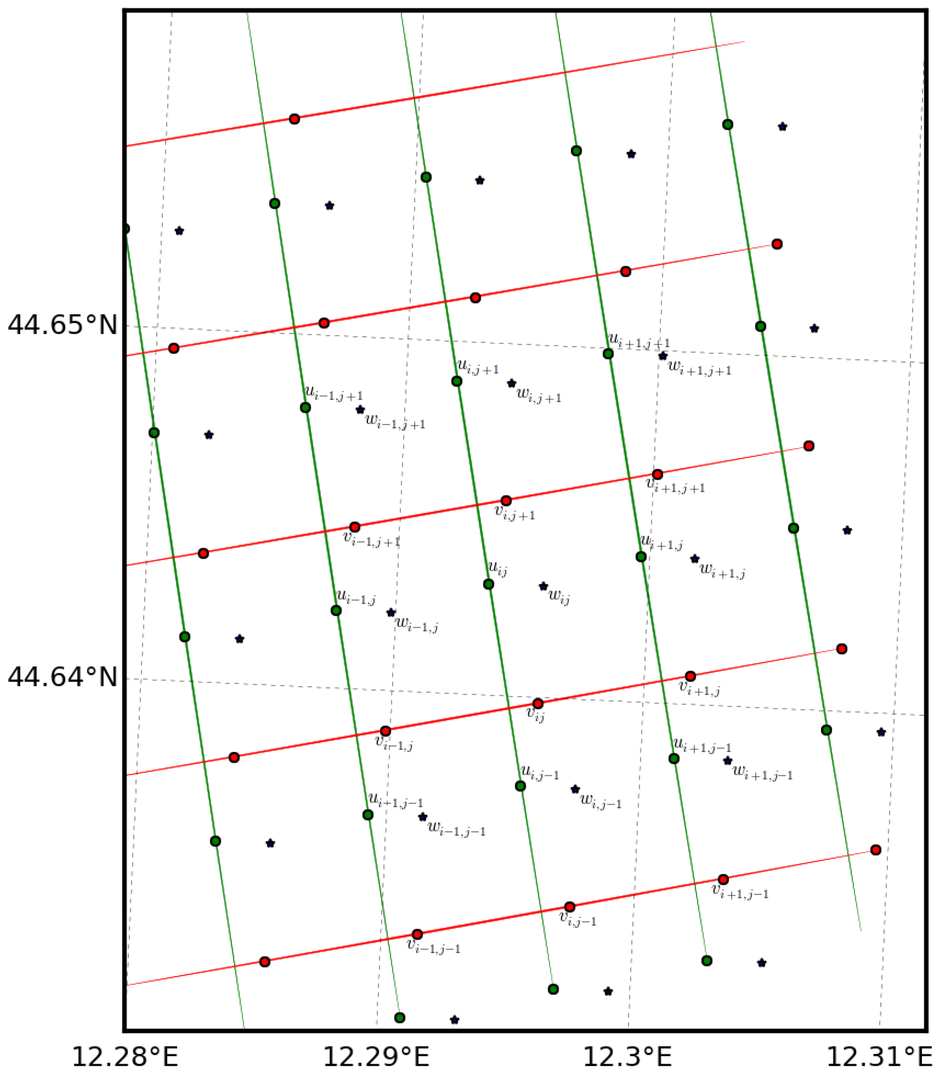
The model data are available in an Arakawa-C grid, with vector quantities, i.e., meridional and zonal components of the velocity, located on the edges of the cell, while the scalar quantities and the vertical component of the velocity are located inside the cell (Figure 3).

On the other hand, the Level-2 MERIS data are available on a swath-based grid. To harmonise all the quantities, we projected the $\rho$ concentration field on all three different grids: the grid of the u-points, on the “west” and “east” edges of the cells; the grid of the v-points, on the “north” and “south” edges of the cells; and the grid of the w-points, in the centres of the cells. The vertical component of the velocity (w) is considered by the model as one of the scalar quantities, such as temperature, salinity and elevation.

The computation of the x and y components of the 2D sediment flux, i.e., the vertical integrals

$$q_{sx}={\int }_{b(x,y)}^0\rho u\mathrm{d}z$$

$$q_{sy}={\int }_{b(x,y)}^0\rho v\mathrm{d}z$$

were performed on the cells’ edges, by means of a simple trapezoidal rule, on every point $(x,y)$ of the horizontal grid:

$$\begin{array}{cc}\hfill & q_{sx}={\int }_{b(x,y)}^0\rho u\mathrm{d}z=\rho {\int }_{b(x,y)}^{0}u\mathrm{d}z\approx -\rho \sum _{k=0}^{N-1}\frac{u\left(z_{k+1}\right)+u\left(z_k\right)}{2}\left(z_{k+1}-z_k\right)\hfill \\ \hfill & q_{sy}={\int }_{b(x,y)}^0\rho v\mathrm{d}z=\rho {\int }_{b(x,y)}^{0}v\mathrm{d}z\approx -\rho \sum _{k=0}^{N-1}\frac{v\left(z_{k+1}\right)+v\left(z_k\right)}{2}\left(z_{k+1}-z_k\right)\hfill \end{array}$$

(11)

where $N=100$ is the number of vertical levels of the grid. The minus sign is because $k=0$ means the surface, thus we integrated from surface downwards.

We now have a 2D sediment flux, whose components were computed on the cells’ edges: the zonal component on the u-points and the meridional component on the v-points.

According to Hyman et al. [38], to approximate the divergence of the sediment flux, we used a local version of the divergence theorem, applied at every single cell of the grid:

$${\left(\overline{\overline{{\nabla }_H·{\overrightarrow{q}}_s}}\right)}_{ij}=\frac{1}{A_{ij}}{\int }_{{\Omega }_{ij}}{\nabla }_H·{\overrightarrow{q}}_s\mathrm{d}\Omega =\frac{1}{A_{ij}}{\int }_{\partial {\Omega }_{ij}}{\overrightarrow{q}}_s·\overrightarrow{n}\mathrm{d}l$$

(12)

where ${\Omega }_{ij}$ is the $ij$ 2D cell, $A_{ij}$ is its area, $\partial {\Omega }_{ij}$ is its frontier, and ${\overrightarrow{q}}_s$ is the 2D sediment flux.

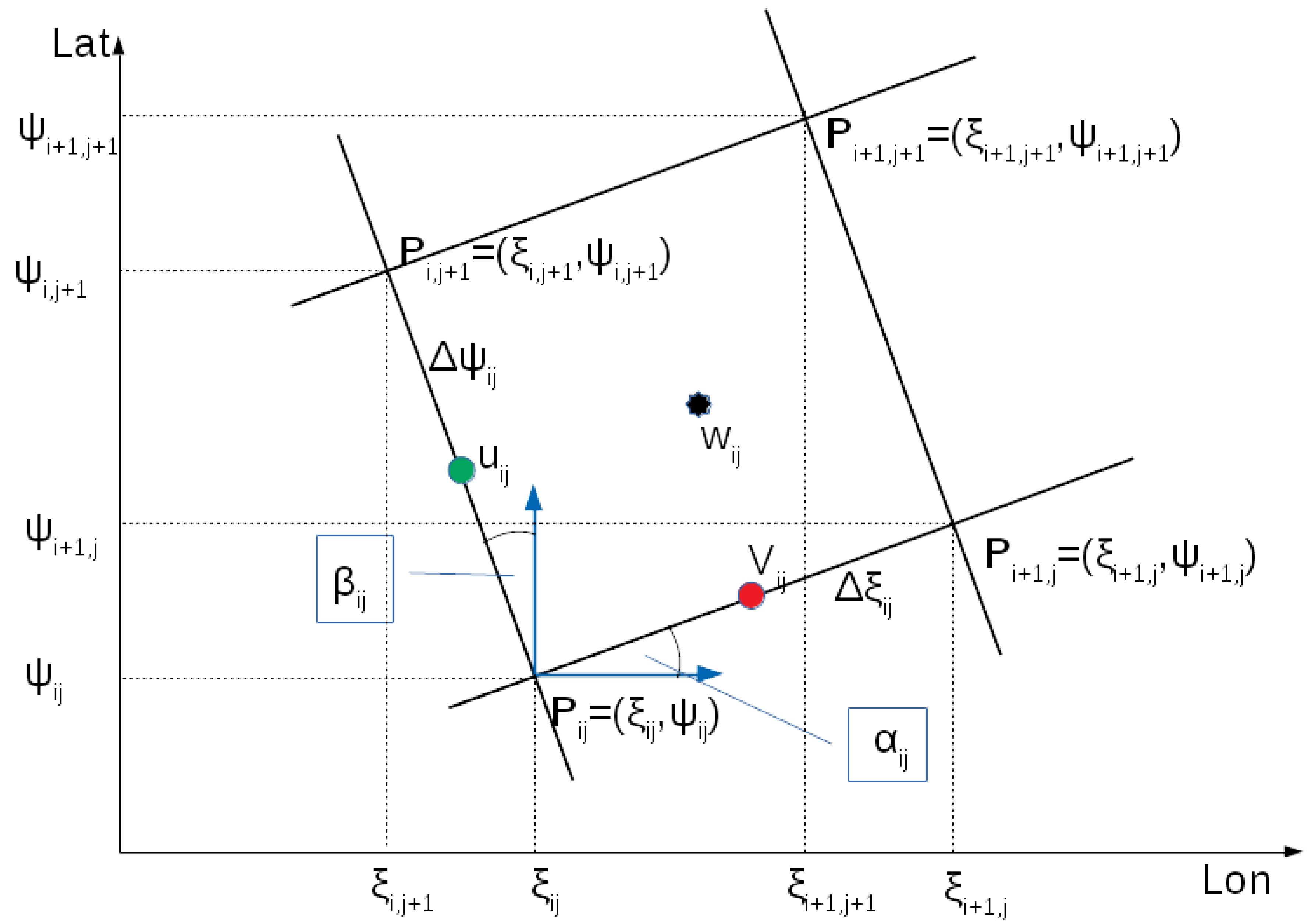
According to Figure 4, we call ${\mathbf{P}}_{ij}=({\xi }_{ij},{\psi }_{ij})$ the southern-most vertex of the $ij$ cell, and ${\xi }_{ij}$ and ${\psi }_{ij}$ its longitude and its latitude.

Let us call also

$$\begin{array}{cc}\hfill & \Delta {\xi }_{ij}=∥{\mathbf{P}}_{i+1,j}-{\mathbf{P}}_{ij}∥\hfill \\ \hfill & \Delta {\psi }_{ij}=∥{\mathbf{P}}_{i,j+1}-{\mathbf{P}}_{ij}∥\hfill \end{array}$$

(13)

the length of the edges of cell $ij$, again as depicted in Figure 4.

Let us call ${\alpha }_{ij}$ the angle between the edge $\overline{{\mathbf{P}}_{ij}{\mathbf{P}}_{i+1,j}}$ and the parallel passing by ${\mathbf{P}}_{ij}$ and ${\beta }_{ij}$ the angle between the edge $\overline{{\mathbf{P}}_{ij}{\mathbf{P}}_{i,j+1}}$ and the meridian passing by ${\mathbf{P}}_{ij}$

The area of the cell $A_{ij}$ can be calculated by:

$$A_{ij}=\Delta {\xi }_{ij}\Delta {\psi }_{ij}sin\left({\widehat{\mathbf{P}}}_{ij}\right)=\Delta {\xi }_{ij}\Delta {\psi }_{ij}cos({\alpha }_{ij}-{\beta }_{ij})$$

(14)

where ${\widehat{\mathbf{P}}}_{ij}$ is the angle in ${\mathbf{P}}_{ij}$ between the segments $\overline{{\mathbf{P}}_{ij}{\mathbf{P}}_{i+1,j}}$ and $\overline{{\mathbf{P}}_{ij}{\mathbf{P}}_{i,j+1}}$. The Winter2012 grid is non-uniform and curvilinear but locally orthogonal, thus ${\alpha }_{ij}=\beta ij$, but in general this may not be the case.

The flux across the border of the $ij$ cell can be decomposed in the four fluxes across the four different edges of the cell. As the edges of the cells are not parallel to meridians and parallels, we have to take into account both components of the velocity field on any edge. Thus, to compute the divergence we rewrite Equation (12) as:

$$\begin{array}{cc}\hfill & A_{ij}·{\left(\overline{\overline{{\nabla }_H·{\overrightarrow{q}}_s}}\right)}_{ij}=\Delta {\xi }_{ij}\Delta {\psi }_{ij}cos({\alpha }_{ij}-{\beta }_{ij}){\left(\overline{\overline{{\nabla }_H·{\overrightarrow{q}}_s}}\right)}_{ij}=\hfill \\ \hfill =& {\int }_{\partial {\Omega }_{ij}}{\overrightarrow{q}}_s·\overrightarrow{n}\mathrm{d}l=\hfill \\ \hfill =& +(-u_{ij}cos{\beta }_{ij}-v_{ij}sin{\beta }_{ij}){\rho }_{ij}^{\left(u\right)}\Delta {\psi }_{ij}+\hfill \\ \hfill & +(-v_{ij}cos{\alpha }_{ij}+u_{ij}sin{\alpha }_{ij}){\rho }_{ij}^{\left(v\right)}\Delta {\xi }_{ij}+\hfill \\ \hfill & +(u_{i+1,j}cos{\beta }_{i+1,j}+v_{i+1,j}sin{\beta }_{i+1,j}){\rho }_{i+1,j}^{\left(u\right)}\Delta {\psi }_{i+1,j}+\hfill \\ \hfill & +(v_{i,j+1}cos{\alpha }_{i,j+1}-u_{i,j+1}sin{\alpha }_{i,j+1}){\rho }_{i,j+1}^{\left(v\right)}\Delta {\xi }_{i+1,j}\hfill \end{array}$$

(15)

where ${\rho }_{ij}^{\left(u\right)}$ and ${\rho }_{ij}^{\left(v\right)}$ are the projection of the tsm_conc field on the u-point and on the v-point, respectively, of cell $ij$; and and $u_{ij}$ and $v_{ij}$ are the bi-dimensional velocities, i.e., the vertically integrated velocities computed in Equation (11), again for cell $ij$:

$$\begin{array}{cc}\hfill & u_{ij}=-\sum _{k=0}^{N-1}\frac{u_{i,j,k+1}+u_{ijk}}{2}\left(z_{k+1}-z_k\right)\hfill \\ \hfill & v_{ij}=-\sum _{k=0}^{N-1}\frac{v_{i,j,k+1}+v_{ijk}}{2}\left(z_{k+1}-z_k\right)\hfill \end{array}$$

(16)

The whole computation is than arranged as per the following flow:

• Vompute ${\xi }_{ij}$ and ${\psi }_{ij}$, coordinates of the vertexes ${\mathbf{P}}_{ij}$ of the cells.
• Compute angles ${\alpha }_{ij}$ and ${\beta }_{ij}$.
• Start a DAILY cycle: at each day compute $u_{ij}$ and $v_{ij}$ according to Equation (16) and then compute the flux divergence ${\left(\overline{\overline{{\nabla }_H·{\overrightarrow{q}}_s}}\right)}_{ij}$ according to Equation (15).
• Compute temporal average of the flux divergence ${\left(\overline{\overline{{\nabla }_H·{\overrightarrow{q}}_s}}\right)}_{ij}$.

3. Results and Discussion

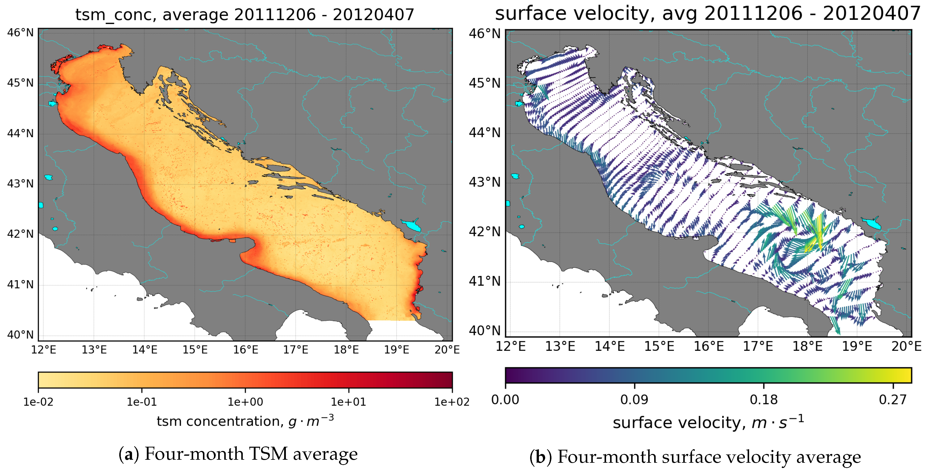
By using a sediment mass balance approach (i.e. the Exner equation, Equation (2)), and thus, by mapping the divergence of the sediment flux, we intend to recognise those zones that are characterised by sediment deposition or erosion. All this does not depend on the specific grain-size (i.e., settling velocity) of the suspended sediment. That is, if a sediment laden pixel does not conserve its sediment concentration along its motion (regardless its grain-size), this necessarily means that some sediment has been lost or gained. In Figure 5, we show the average, over the whole time frame under investigation (four months, from 6 December 2011 to 7 April 2012), of our input fields: the satellite TSM (Total Suspended Matter) concentration field and the surface velocity field. The Western Adriatic Coastal Current (WACC) is clearly visible along the Italian shoreline, from both the TSM and the velocity patterns.

We notice that the TSM satellite product, for the study period, highlights the riverine input along the northern Adriatic coast (see Figure 5a), which significantly contributes in driving a southeastward current along the Italian coast. In particular, Figure 5a shows that the Po, along with all the other North Adriatic river inputs, produces an almost single river plume, contributing 84% of the total freshwater discharge delivered to the basin [39,40]. We recognise the presence of mid-to-high TSM concentration waters, in the entire northern basin and, partly, in the middle part of the Adriatic Sea. For the cold period we analysed, high TSM values are also recorded at the exit to the Ionian Sea, through the Otranto Strait [7]. Finally, we remark that the spatial distribution of optically complex waters, marked by high turbidity parameters such as TSM or a diffusion attenuation coefficient, closely matches slow-settling particle deposition patterns of the Adriatic Sea [7], and thus highlights zones that are affected by sedimentary processes.

Accordingly, the highly resolved marine currents, provided by the MITgcm numerical outputs, show the correct alongshore momentum (Figure 5b), where the inclusion of lateral freshwater inputs affects the capability to reproduce buoyant processes in the coastal area. The model output confirms, for the winter season, a basin-wide cyclonic circulation with a strong southward currents along the Italian Peninsula on the western side (i.e., the WACC). Such a geostrophic pattern is known to be due to the estuarine circulation [41], forced by river inputs, mainly the Po River, and by strong air–sea fluxes. In particular, the Po River input results in a wide extension of surface freshwater, particularly evident along the northern littoral of the basin [24]. Between the Po River mouth and the Conero Promontory (Figure 5b), the WACC width is about 40 km and its maximum speed reaches 0.25 $\mathrm{m} {\mathrm{s}}^{-1}$. This well-recognisable, southeastward current along the Italian coast (i.e., the WACC), overlays the TSM pattern, providing a comforting agreement between the satellite and the numerical upstream data. Moreover, for the study period, the effect of surface wind stress (i.e., the Bora event recorded from 25 January to 14 February 2012) led to a more confined strip of freshwater [24].

On the western Adriatic coast, Bora is a downwelling favourable wind and can generate large waves with significant wave heights of 1 m, and period of 5 s [42]. Wave-driven sediment resuspension is an important resuspension mechanism in the shallow coastal areas of the NAS [43], and contributes significantly to the complexity of the sediment distribution and flux features in the region. Therefore, waves should not be neglected in the study of dynamics of sediment transport and resuspension in the shallow coastal seas. However, the fact that the hydrologic model we used does not include waves did not affect our ability to estimate suspended sediment concentration, which is directly retrieved from satellite, regardless of the mechanism that keep the sediment in suspension. Moreover, sediment transport is known to be insensitive to the angle between directions of wave propagation and current in the NAS, where large waves were generated by the Bora storm for strong wave conditions [44,45]. This suggests that wave-induced currents, not included in the MITgcm runs, have no significant effect on the southward sediment flux along the western Adriatic coast. Finally, it is worth mentioning that the effect of mixing due to wave breaking on sediment distribution and fluxes in the NAS is not significant since the water column is well mixed due to strong current shear driven by the Bora winds and shallow water depth [45].

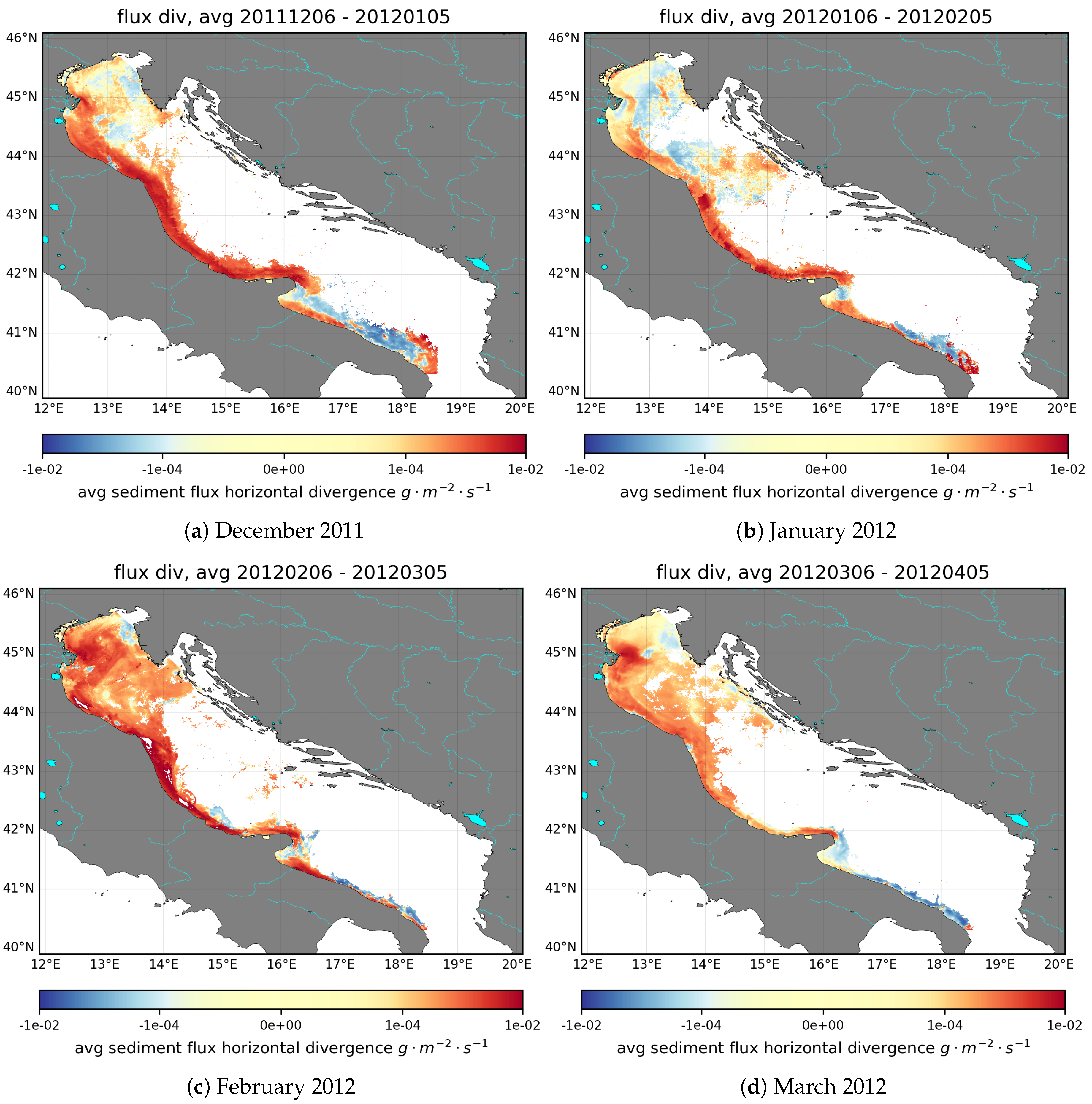
In Figure 6, from Figure 6a to Figure 6d, on the other hand, we show the sediment flux divergence fields obtained with the methodology introduced in Section 2.3. For an easier readability of the computed maps, monthly averages are shown, i.e., one map for each of the months under investigation: December 2011, January 2012, February 2012 and March 2012. From Equation (2), a pixel (a cell) with positive divergence (a yellow or a red pixel) means a sediment erosion point, or, more correctly, a point where we have sediment from the bottom layer entrained into the water flow. Conversely a pixel (a cell) with negative divergence (a blue or light blue pixel) means a sediment deposition point, or a point where suspended sediment is precipitating on the bottom layer.

A long-time scale persistence of erosive or depositional pattern along the coastal plume can be related to sediment starvation or sediment availability over the inner shelf (Figure 6). Indeed, for the time frame under observation, we found a persistent sediment erosion condition along the coast traits between the Po river delta and the Conero promontory and between the Conero and Gargano rocky promontories (Figure 6). This, in general, is in agreement with the overall shoreline retrograding shape reported by ISPRA [46] and ISPRA [47], found in [48]. On the other hand, there are depositional patterns in the Gulf of Manfredonia, likely due to recirculation of the southern Adriatic currents around the Gargano promontory, as depicted in [49,50]. The Po river delta shows depositional and erosive behaviours, depending on the season. In this area, the availability of long time series of both observation and model data would help identify the predominant long-term behaviour.

A further confirmation of our results can be obtained from the knowledge of the subaqueous clinoform anatomy [51]. In particular, we can use our computed divergence patterns as a proxy for the thickness of subaqueous clinoform: clinoform thicknesses are expected to decrease within our computed erosional zones and to increase where we estimate sediment deposition. According to Correggiari et al. [51] (see Figure 2 in [51], reported also in [12,45]), we infer that our depositional areas, e.g., south of the Po River delta and south of the Gargano promontory, correspond to those areas where the highest clinoform thickness is observed to be attached to the shoreline.

Finally, we remark that, in the Adriatic Sea, the majority of horizontal structures that are observed in the coastal zone are characterised by Rossby and Richardson numbers of around 1 (sub-mesoscale), representing areas where vertical fluxes and buoyancy are enhanced [52]. In such a complex environment, sudden changes in the wind forcing can trigger strong hydrodynamic events, such as the formation of dense water (DW) and wind driven upwelling. In the model we used, the direct effect of wind forcing is assimilated in order to reproduce DW formation events [24] as well as a number of small scale features that show high horizontal variability of vertical processes. This proves that the high resolution of MITgcm allows for the reproduction of more small scale vortical structures, identifying a wider spatial range of processes. Therefore, pairing high resolution TSM fields from remote sensing with the MITgcm outputs, which well represent submesoscale processes, made us confident in capturing coastal sediment transport dynamics.

As already pointed out, waves play a major role in sediment suspension and resuspension (see [45] for a study on the Adriatic sea). While MITgcm based simulations do not include waves, their effect in sediment suspension is taken into account in the observation dataset, i.e., in the satellite provided TSM maps. The availability of such dataset, furthermore, allows us to avoid the execution of a sediment dynamics model. The goal of our work is to investigate the feasibility of an operative product that, with a low computational effort, can represent the sediment dynamics at basin or regional spatial scales, and at decadal time scales. The observational-numerical approach we propose, at these spatial and temporal scales, with these spatial and temporal resolutions, appears quite adequate to fulfil this objective.

4. Conclusions

This work proposes a new approach to investigate the sediment erosive and depositional patterns that occur at regional or basin scale, and that are driven by mesoscale and sub-mesoscale processes, such as coastal currents and fluvial plumes. Our approach is based on a synergy between satellite observations and numerical simulations. The computed maps of the sediment flux divergence show patterns of sediment erosion and deposition that are in agreement with the general knowledge of the sediment dynamics and coastal geomorphology in the Adriatic Sea.

The main agents in the sediment distribution on the shore, and the subsequent morphodynamics, are waves and wave-induced currents. However, the daily Total Suspended Matter as retrieved from Ocean Colour remote sensing is able to capture the material resuspended by a large variety of phenomena (including wave-induced resuspension). We therefore believe that the divergence of the sediment flux, estimated from the synergy of remote sensing and high resolution horizontal marine currents, is able to highlight both depositional and erosive areas resulting from mass conservation, i.e., those pixel where we can expect sediment deposition/erosion over the continental shelf, regardless of what caused its deposition or entrainment.

Our investigation was limited by the short intersection of the two time domains: the Coastcolour project time domain (from 4 January 2003 to 7 April 2012) and the Winter2012 model run time domain (from 6 December 2011 to 30 April 2012). The short duration of this intersection (i.e., four months) did not allow us to provide statistical analyses and further validation of our results. However, the use of the two upstream datasets, as well as the remapping and interpolation schemes, resulted to be suitable tools for the detection of realistic depositional or erosive spatial patterns, which were confirmed by the authors of [12,49,50]. We finally remark that the goal of our work is to provide a potential operative product that might be suitable for long-term analyses and monitoring programmes.

A longer, multi-year duration would allow one to extract trend analysis that could be matched with the long time series of in-situ information on the Adriatic shoreline. This time series of in-situ information is the “ground truth” that can validate and tell the accuracy of the methodology that has been introduced.

In envisioning a longer time frame, a suitable observational part (i.e., spaceborne remotely sensed data) can be represented by the 2002–2012 and 2016-onward TSM time series from either Coastcolour [28] or OLCI [53], with daily time resolution and 300-m spatial resolution. A further application of our approach could also be the design and use of ad hoc models, which could assimilate the sediment concentration from the satellite measurements, as done by Stroud et al. [15] for Lake Michigan, and that directly output the divergence field.

Finally, it would be promising to consider the assimilation of two other kinds of spaceborne sensors: geostationary satellite and hyperspectral missions. Geostationary sensors such as SEVIRI–Meteosat [54] and their successors show a very high temporal resolution (15 min–1 h), at the expenses of a very coarse spatial resolution, e.g., 4 km × 6 km at our latitudes). On the contrary, hyper-spectral missions (PRISMA [55] and EnMAP [56]) show coarser temporal resolution, but much finer spatial and spectral resolutions. The high temporal resolution of geostationary satellites can enhance the near daily temporal resolution of Low Earth Orbit satellites and mitigate the presence of cloud coverage, while the high spectral resolution of hyperspectral sensors can give insight on the chemical composition of the sediment as well as on its size distribution.

References

- Dyer, K. Coastal and Estuarine Sediment Dynamics; Wiley: New York, NY, USA, 1986. [Google Scholar]
- Masselink, G.; Hughes, M.G. An Introduction to Coastal Processes and Geomorphology; Routledge: Abingdon, UK, 2014. [Google Scholar]
- Syvitski, J.P.M.; Harvey, N.; Wolanski, E.; Burnett, W.C.; Perillo, G.M.E.; Gornitz, V. Dynamics of the coastal zone. In Coastal Change and the Anthropocene: The Land-Ocean Interactions in the Coastal Zone Project of the International Geosphere-Biosphere Programme; Crossland, C.J., Kremer, H.H., Lindeboom, H.J., Crossland, J.I.M., Le Tissier, M.D.A., Eds.; Global Change—The IGBP Series; Springer: Texel, The Netherlands, 2005; pp. 39–94. [Google Scholar]
- Carniello, L.; Silvestri, S.; Marani, M.; D’Alpaos, A.; Volpe, V.; Defina, A. Sediment dynamics in shallow tidal basins: In situ observations, satellite retrievals, and numerical modeling in the Venice Lagoon. J. Geophys. Res. Earth Surf. 2014, 119, 802–815. [Google Scholar] [CrossRef]
- Parker, G.; Garcia, M. Theory for a clinoform of permanent form on a continental margin emplaced by weak, dilute muddy turbidity currents. In Proceedings of the 4th IAHR Symposium on River, Coastal and Estuarine Morphodynamics (RCEM 2005), Urbana, IL, USA, 4–7 October 2005; Taylor and Frances: Philadelphia, PA, USA, 2006; pp. 553–561. [Google Scholar]
- Fagherazzi, S.; Overeem, I. Models of deltaic and inner continental shelf landform evolution. Annu. Rev. Earth Planet. Sci. 2007, 35, 685–715. [Google Scholar] [CrossRef]
- Bignami, F.; Sciarra, R.; Carniel, S.; Santoleri, R. Variability of Adriatic Sea coastal turbid waters from SeaWiFS imagery. J. Geophys. Res. Oceans 2007, 112. [Google Scholar] [CrossRef]
- Brando, V.; Braga, F.; Zaggia, L.; Giardino, C.; Bresciani, M.; Matta, E.; Bellafiore, D.; Ferrarin, C.; Maicu, F.; Benetazzo, A.; et al. High-resolution satellite turbidity and sea surface temperature observations of river plume interactions during a significant flood event. Ocean Sci. 2015, 11, 909–920. [Google Scholar] [CrossRef]
- Cattaneo, A.; Trincardi, F.; Asioli, A.; Correggiari, A. The Western Adriatic shelf clinoform: energy-limited bottomset. Cont. Shelf Res. 2007, 27, 506–525. [Google Scholar] [CrossRef]
- Sherwood, C.R.; Book, J.W.; Carniel, S.; Cavaleri, L.; Chiggiato, J.; Das, H.; Doyle, J.D.; Harris, C.K.; Niedoroda, A.W.; Perkins, H. Sediment Dynamics in the Adriatic Sea Investigated with Coupled Models. Oceanography 2004, 17, 58–69. [Google Scholar] [CrossRef]
- Harris, C.K.; Sherwood, C.R.; Signell, R.P.; Bever, A.J.; Warner, J.C. Sediment dispersal in the northwestern Adriatic Sea. J. Geophys. Res. Oceans 2008, 113. [Google Scholar] [CrossRef]
- Pellegrini, C.; Maselli, V.; Cattaneo, A.; Piva, A.; Ceregato, A.; Trincardi, F. Anatomy of a compound delta from the post-glacial transgressive record in the Adriatic Sea. Mar. Geol. 2015, 362, 43–59. [Google Scholar] [CrossRef]
- Poulain, P.M. Adriatic Sea surface circulation as derived from drifter data between 1990 and 1999. J. Mar. Syst. 2001, 29, 3–32. [Google Scholar] [CrossRef]
- Ouillon, S.; Douillet, P.; Andréfouët, S. Coupling satellite data with in situ measurements and numerical modeling to study fine suspended-sediment transport: a study for the lagoon of New Caledonia. Coral Reefs 2004, 23, 109–122. [Google Scholar]
- Stroud, J.R.; Lesht, B.M.; Schwab, D.J.; Beletsky, D.; Stein, M.L. Assimilation of satellite images into a sediment transport model of Lake Michigan. Water Resour. Res. 2009, 45. [Google Scholar] [CrossRef]
- Niedoroda, A.W.; Reed, C.W.; Das, H.; Fagherazzi, S.; Donoghue, J.F.; Cattaneo, A. Analyses of a large-scale depositional clinoformal wedge along the Italian Adriatic coast. Mar. Geol. 2005, 222, 179–192. [Google Scholar] [CrossRef]
- Exner, F.M. Uber die wechselwirkung zwischen wasser und geschiebe in flussen. Akad. Wiss. Wien Math. Naturwiss. Klasse 1925, 134, 165–204. [Google Scholar]
- Exner, F.M. Zur Physik der Dünen; Hölder: Wien, Austria, 1920. [Google Scholar]
- Paola, C.; Voller, V. A generalized Exner equation for sediment mass balance. J. Geophys. Res. Earth Surf. 2005, 110. [Google Scholar] [CrossRef]
- Komar, P.D. The mechanics of sand transport on beaches. J. Geophys. Res. 1971, 76, 713–721. [Google Scholar] [CrossRef]
- Rosati, J.; Walton, T.; Bodge, K. Longshore sediment transport. In Coastal Engineering Manual; USACE: Washington, DC, USA, 2002. [Google Scholar]
- Ashton, A.; Murray, A.B.; Arnoult, O. Formation of coastline features by large-scale instabilities induced by high-angle waves. Nature 2001, 414, 296–300. [Google Scholar] [CrossRef] [PubMed]
- Ashton, A.D.; Murray, A.B. High-angle wave instability and emergent shoreline shapes: 1. Modeling of sand waves, flying spits, and capes. J. Geophys. Res. Earth Surf. (2003–2012) 2006, 111. [Google Scholar] [CrossRef]
- McKiver, W.; Sannino, G.; Braga, F.; Bellafiore, D. Investigation of model capability in capturing vertical hydrodynamic coastal processes: A case study in the north Adriatic Sea. Ocean Sci. 2016, 12, 51. [Google Scholar] [CrossRef]
- D’Sa, E.J.; Miller, R.L.; McKee, B.A. Suspended particulate matter dynamics in coastal waters from ocean color: Application to the northern Gulf of Mexico. Geophys. Res. Lett. 2007, 34. [Google Scholar] [CrossRef]
- Dogliotti, A.I.; Ruddick, K.; Nechad, B.; Doxaran, D.; Knaeps, E. A single algorithm to retrieve turbidity from remotely-sensed data in all coastal and estuarine waters. Remote Sens. Environ. 2015, 156, 157–168. [Google Scholar] [CrossRef]
- Nechad, B.; Ruddick, K.; Park, Y. Calibration and validation of a generic multisensor algorithm for mapping of total suspended matter in turbid waters. Remote Sens. Environ. 2010, 114, 854–866. [Google Scholar] [CrossRef]
- ESA. MERIS Instrument for Remote Sensing of the Coastal Zone. Available online: http://www.coastcolour.info (accessed on 18 June 2019).
- MITgcm Group. MITgcm Website. Available online: http://mitgcm.org (accessed on 19 July 2019).
- ESA. MERMAID—Meris Matchup In-Situ Database. Available online: http://mermaid.acri.fr/ (accessed on 15 July 2019).
- Sánchez-Garrido, J.C.; Sannino, G.; Liberti, L.; García Lafuente, J.; Pratt, L. Numerical modeling of three-dimensional stratified tidal flow over Camarinal Sill, Strait of Gibraltar. J. Geophys. Res. Oceans 2011, 116. [Google Scholar] [CrossRef]
- Sannino, G.; Sanchez Garrido, J.; Liberti, L.; Pratt, L. Exchange Flow through the Strait of Gibraltar as Simulated by a σ-Coordinate Hydrostatic Model and az-Coordinate Nonhydrostatic Model. In The Mediterranean Sea: Temporal Variability and Spatial Patterns; John Wiley & Sons: New York, NY, USA; pp. 25–50.
- Drofa, O.; Malguzzi, P. In Proceedings of the 14th International Conference on Clouds and Precipitation, Bologna, Italy, 19–23 July 2004. Available online: https://www.sciencedirect.com/journal/atmospheric-research/vol/82/issue/1 (accessed on 13 May 2019).
- Malguzzi, P.; Grossi, G.; Buzzi, A.; Ranzi, R.; Buizza, R. The 1966 “century” flood in Italy: A meteorological and hydrological revisitation. J. Geophys. Res. Atmos. 2006, 111. [Google Scholar] [CrossRef]
- Ferrarin, C.; Roland, A.; Bajo, M.; Umgiesser, G.; Cucco, A.; Davolio, S.; Buzzi, A.; Malguzzi, P.; Drofa, O. Tide-surge-wave modelling and forecasting in the Mediterranean Sea with focus on the Italian coast. Ocean Model. 2013, 61, 38–48. [Google Scholar] [CrossRef] [Green Version]
- Raspaud, M.; Hoese, D.; Dybbroe, A.; Lahtinen, P.; Devasthale, A.; Itkin, M.; Hamann, U.; rum Rasmussen, L.; Nielsen, E.S.; Leppelt, T.; et al. PyTroll: An open source, community driven Python framework to process Earth Observation satellite data. Bull. Am. Meteorol. Soc. 2018, 99, 1329–1336. [Google Scholar] [CrossRef] [Green Version]
- EMODnet Bathymetry Consortium. EMODnet Digital Bathymetry (DTM). EMODnet Bathymetry 2016. 2016. Available online: https://doi.org/10.12770/c7b53704-999d-4721-b1a3-04ec60c87238 (accessed on 19 July 2019).
- Hyman, J.M.; Knapp, R.J.; Scovel, J.C. High order finite volume approximations of differential operators on nonuniform grids. Phys. D Nmiscar Phenomena 1992, 60, 112–138. [Google Scholar] [CrossRef]
- Cozzi, S.; Giani, M. River water and nutrient discharges in the Northern Adriatic Sea: Current importance and long term changes. Cont. Shelf Res. 2011, 31, 1881–1893. [Google Scholar] [CrossRef]
- Falcieri, F.M.; Benetazzo, A.; Sclavo, M.; Russo, A.; Carniel, S. Po River plume pattern variability investigated from model data. Cont. Shelf Res. 2014, 87, 84–95. [Google Scholar] [CrossRef]
- Hopkins, T.; Artegiani, A.; Kinder, C.; Pariante, R. A discussion of the northern Adriatic circulation and flushing as determined from the ELNA hydrography. In The Adriatic Sea; European Commission: Brussels, Belgium, 1999; Volume 32, pp. 85–106. [Google Scholar]
- Cavaleri, L.; Bertotti, L. In search of the correct wind and wave fields in a minor basin. Mon. Weather Rev. 1997, 125, 1964–1975. [Google Scholar] [CrossRef]
- Wang, X.; Pinardi, N. Modeling the dynamics of sediment transport and resuspension in the northern Adriatic Sea. J. Geophys. Res. Oceans 2002, 107. [Google Scholar] [CrossRef]
- Grant, W.D.; Madsen, O.S. Combined wave and current interaction with a rough bottom. J. Geophys. Res. Oceans 1979, 84, 1797–1808. [Google Scholar] [CrossRef]
- Wang, X.; Pinardi, N.; Malacic, V. Sediment transport and resuspension due to combined motion of wave and current in the northern Adriatic Sea during a Bora event in January 2001: A numerical modelling study. Cont. Shelf Res. 2007, 27, 613–633. [Google Scholar] [CrossRef]
- ISPRA. MARE E AMBIENTE COSTIERO. Available online: http://www.isprambiente.gov.it/files/pubblicazioni/statoambiente/tematiche2011/05_%20Mare_e_ambiente_costiero_2011.pdf (accessed on 13 May 2019).
- ISPRA. MARE E AMBIENTE COSTIERO. Available online: http://www.isprambiente.gov.it/files/pubblicazioni/statoambiente/tematiche-2012/Cap.5_Mare_ambiente_costiero.pdf (accessed on 13 May 2019).
- ISPRA. Pubblicazioni ISPRA—Stato Ambiente. Available online: http://www.isprambiente.gov.it/files/pubblicazioni/statoambiente (accessed on 13 May 2019).
- Artegiani, A.; Paschini, E.; Russo, A.; Bregant, D.; Raicich, F.; Pinardi, N. The Adriatic Sea general circulation. Part II: baroclinic circulation structure. J. Phys. Oceanogr. 1997, 27, 1515–1532. [Google Scholar] [CrossRef]
- Limic, N.; Orlic, M. Objective analysis of geostrophic currents in the Adriatic Sea. Geofizika 1986, 3, 75–84. [Google Scholar]
- Correggiari, A.; Trincardi, F.; Langone, L.; Roveri, M. Styles of failure in late Holocene highstand prodelta wedges on the Adriatic shelf. J. Sediment. Res. 2001, 71, 218–236. [Google Scholar] [CrossRef]
- Thomas, L.N.; Tandon, A.; Mahadevan, A. Submesoscale processes and dynamics. Ocean Model. Eddying Regime 2008, 177, 17–38. [Google Scholar]
- ESA. OLCI Instrument. 2016. Available online: https://sentinel.esa.int/web/sentinel/technical-guides/sentinel-3-olci/olci-instrument (accessed on 13 June 2019).
- Aminou, D. MSG’s SEVIRI instrument. ESA Bull. (0376-4265) 2002, 111, 15–17. [Google Scholar]
- Lopinto, E.; Ananasso, C. The Prisma Hyperspectral Mission. In Proceedings of the 33rd EARSeL Symposium Towards Horizon 2020, Matera, Italy, 3–6 June 2013. [Google Scholar]
- Stuffler, T.; Kaufmann, C.; Hofer, S.; Förster, K.; Schreier, G.; Mueller, A.; Eckardt, A.; Bach, H.; Penne, B.; Benz, U.; et al. The EnMAP hyperspectral imager—An advanced optical payload for future applications in Earth observation programmes. Acta Astronaut. 2007, 61, 115–120. [Google Scholar] [CrossRef]
Figure 1.
True Colour (bands 9,6,4) image of the Adriatic Sea, 28 February 2019, by the OLCI sensors on board of the Sentinel-3A and Sentinel-3B spacecrafts. The Western Adriatic Coastal Current (yellow arrows) is clearly visible, due to its suspended sediment load, transported along the coast [13]. The North Adriatic Gyre and the subsequent path of the North Adriatic Dense Water are highlighted in orange [13]. The black arrows indicate the geographic locations mentioned in the text.
Figure 2.
Schematic representation of the seabed geometry: represents the sediment concentration in water; D represents the “closure depth”, i.e., the maximum depth at which the waves are able to generate sediment resuspension from the seabed; and represents the seabed height, relative to a fixed datum.
Figure 3.
Grid detail: cell and edge points.
Figure 4.
Geometry of cell.
Figure 5.
Source data: Four-month averages (from 6 December 2011 to 7 April 2012) of surface TSM concentration (a) and surface velocity field (b).
Figure 6.
Monthly averages of sediment flux divergence: (a) December 2011; (b) January 2012; (c) February 2012; and (d) March 2012.
© 2019 by the authors. Licensee MDPI, Basel, Switzerland. This article is an open access article distributed under the terms and conditions of the Creative Commons Attribution (CC BY) license (http://creativecommons.org/licenses/by/4.0/).
Share and Cite
MDPI and ACS Style
Benincasa, M.; Falcini, F.; Adduce, C.; Sannino, G.; Santoleri, R. Synergy of Satellite Remote Sensing and Numerical Ocean Modelling for Coastal Geomorphology Diagnosis. Remote Sens. 2019, 11, 2636. https://doi.org/10.3390/rs11222636
AMA Style
Benincasa M, Falcini F, Adduce C, Sannino G, Santoleri R. Synergy of Satellite Remote Sensing and Numerical Ocean Modelling for Coastal Geomorphology Diagnosis. Remote Sensing. 2019; 11(22):2636. https://doi.org/10.3390/rs11222636
Chicago/Turabian StyleBenincasa, Mario, Federico Falcini, Claudia Adduce, Gianmaria Sannino, and Rosalia Santoleri. 2019. "Synergy of Satellite Remote Sensing and Numerical Ocean Modelling for Coastal Geomorphology Diagnosis" Remote Sensing 11, no. 22: 2636. https://doi.org/10.3390/rs11222636
Note that from the first issue of 2016, this journal uses article numbers instead of page numbers. See further details here.