Purifying SLIC Superpixels to Optimize Superpixel-Based Classification of High Spatial Resolution Remote Sensing Image


1
School of Computer Science, China University of Geosciences, Lumo Road 388, Wuhan 430074, China
2
Department of Geodesy and Geomatics Engineering, CRC-Laboratory in Advanced Geomatics Image Processing, University of New Brunswick, 15 Dineen Drive, Fredericton, NB E3B 5A3, Canada
*
Author to whom correspondence should be addressed.
Remote Sens. 2019, 11(22), 2627; https://doi.org/10.3390/rs11222627
Submission received: 3 October 2019
/
Revised: 1 November 2019
/
Accepted: 7 November 2019
/
Published: 10 November 2019
(This article belongs to the Special Issue Robust Multispectral/Hyperspectral Image Analysis and Classification)
Abstract
:Fast and accurate classification of high spatial resolution remote sensing image is important for many applications. The usage of superpixels in classification has been proposed to accelerate the speed of classification. However, although most superpixels only contain pixels from single class, there are still some mixed superpixels, which mostly locate near the edge of different classes, and contain pixels from more than one class. Such mixed superpixels will cause misclassification regardless of classification methods used. In this paper, a superpixels purification algorithm based on color quantization is proposed to purify mixed Simple Linear Iterative Clustering (SLIC) superpixels. After purifying, the mixed SLIC superpixel will be separated into smaller superpixels. These smaller superpixels are pure superpixels which only contain a single kind of ground object. The experiments on images from the dataset BSDS500 show that the purified SLIC superpixels outperform the original SLIC superpixels on three segmentation evaluation metrics. With the purified SLIC superpixels, a classification scheme in which only edge superpixels are selected to be purified is proposed. The strategy of purifying edge superpixels not only improves the efficiency of the algorithm, but also improves the accuracy of the classification. The experiments on a remote sensing image from WorldView-2 satellite demonstrate that purified SLIC superpixels at all scales can generate classification result with higher accuracy than original SLIC superpixels, especially at the scale of , for which the accuracy increase is higher than 4%.
1. Introduction
In recent decades, the available technologies for Earth observation generate a lot of high spatial resolution airplane and satellite images. However, the huge number of generated remote sensing image data needs to be processed and analyzed for various purposes [1,2,3]. The classification of high spatial resolution remote sensing data is a crucial step for processing these data. Nonetheless, it is still a challenge to classify the data accurately and efficiently in practical applications.
In the high spatial resolution remote sensing images, the spatial information is abundant and the spectral information is complex [4]. Therefore, the traditional pixel based classification algorithm that cannot make full use of the spatial information is not the best choice for the classification task. The object based image analysis (OBIA), which replaces the pixel with the object containing a group of connected homogeneous pixels, has been developed to better exploit the spatial information in the image [4,5,6]. The object based classification has a lot of advantages over the pixel based classification in dealing with high spatial resolution imagery [7]. However, the performance of object based classification depends on the segmentation quality. Many segmentation algorithms have been proposed, but segmentation is still a problem in OBIA [5,8,9]. Many segmentation algorithms including the popular multiresolution segmentation [10] have trouble in finding optimal parameters [9,11]. Even objects from the same class may present in different scales. If the scale parameter is too large, under-segmented objects, which negatively influence the classification, will be generated. Therefore, the classification based on over-segmented objects can be a viable alternative to objects, even though the over-segmented objects cannot make good use of the shape information.
Superpixel is a good choice for over-segmentation [12,13]. It was first introduced as a preprocessing step to over-segment an image into small superpixels for simplifying the computation in subsequent stages [14]. The superpixel can carry more information than pixels and adhere better to the natural image boundaries [15,16]. In addition, superpixels can decrease the computation complexity and speed up the subsequent processing [12,13,14]. Moreover, superpixels reduce the susceptibility to noise and outliers, capturing image redundancy [17]. In the field of remote sensing image processing, superpixels have been applied in a diverse range of applications and data types [18,19,20,21,22,23,24,25]. In [13], a classification framework using a superpixel-based graphical model to capture the contextual information and the spatial dependence between the superpixels is proposed. In [26], superpixels were used to define the neighborhood similarity of a pixel adapted to the local characteristics of each image. In [27], a scheme for superpixel description based on Bag of visual Words, which includes information from adjacent superpixels, is introduced. In [28], edge-based processing and superpixel processing were combined for automatic generation of thematic maps for small agricultural parcels. In [29], the Superpixel Contour algorithm was introduced to generate a set of different levels of segmentation for a semi-automatic optimization of object-based classification of multitemporal data. In [1], superpixels were applied in the segmentation and classification of very high resolution remote sensing data.
Many algorithms for generating superpixels have been developed [30]. Among them, six algorithms [12,31,32,33,34,35] were recommended in [30] because these algorithms can be considered stable according to their superior performance regarding boundary recall, under-segmentation error and explained variation. Contour relaxed superpixels [32], Superpixels Extracted via Energy-Driven Sampling [34] and Extended Topology Preserving Segmentation [35] are based on an energy optimization process in which the image is partitioned into a regular grid as initial superpixel segmentation and pixels are exchanged between neighboring superpixels to optimize a formulated energy [30]. Entropy Rate Superpixels [31] is a graph-based algorithm that treats the image as undirected graph and partition this graph based on edge-weights which are often computed as color differences or similarities [30]. Eikonal Region Growing Clustering [33] represents superpixels as evolving contours starting from initial seed pixels [30]. SLIC [12] is a clustering based algorithm inspired by k-means initialized by seed pixels and combining color information and spatial information [30].
However, these algorithms still generate some mixed superpixels which stretch across different objects. The reasons for the mixed superpixels are various. For example, in SLIC algorithm, if the initial cluster centers locate near the boundary, the superpixels related to these cluster centers will include nearby pixels from different objects because the spatial distance and spectral distance are both considered in the clustering process. The classification on mixed superpixels certainly generated incorrect result for some pixels because only one label is assigned to all pixels in the mixed superpixel.
In this paper, a purification algorithm is proposed to purify SLIC superpixels for reducing misclassifications caused by mixed superpixels in the superpixel-based classification. In addition, an efficient scheme to apply the purified SLIC superpixels in the classification is proposed. The mixed SLIC superpixels are divided into small pure superpixels by applying the proposed purification algorithm, which is based on the color quantization [36]. The result of color quantization provides the information for judging whether the SLIC superpixel should be purified and locating new cluster centers for the purifying. With the proposed purification algorithm, the generated superpixels are purer and can preserve more accurate boundary information. The purified SLIC superpixels and original SLIC superpixels generated on images from Berkeley Segmentation Dataset 500 (BSDS500) were compared in three different evaluation metrics to validate the effectiveness of the proposed purification algorithm. The experimental results show that the purified SLIC superpixels perform better than original SLIC superpixels for all evaluation metrics. As for the classification scheme, purifying all superpixels in a large high spatial resolution remote sensing image is unnecessary and some unnecessary purifying may cause misclassification. In the proposed classification scheme, only superpixels which are in the group of edge superpixels are considered for purifying. In this way, most superpixels that do not need to be purified can be excluded for purifying process. To demonstrate that the purified SLIC superpixels can provide a more accurate basis for subsequent process, the proposed classification scheme was compared with the classification based on the SLIC superpixels in classification accuracy. In addition, the classification accuracy of the proposed scheme and the scheme which purifies all SLIC superpixels were compared to show that purifying all SLIC superpixels is unnecessary and may cause the loss of classification accuracy. The experimental results show that the classification based on purified SLIC superpixels in different scales can get higher accuracy than classification based on original SLIC superpixels and the scheme of purifying all SLIC superpixels indeed causes the loss of classification accuracy.
2. Background and Methods
2.1. Simple Linear Iterative Clustering (SLIC) Superpixels
Among various algorithms proposed to generate superpixels, SLIC has been proved to be on the list of algorithms showing superior performance [30] regarding metrics such as boundary recall, under-segmentation error, and explained variation. It also shows advantages in simplicity, adherence to boundaries, computational speed and memory efficiency. SLIC is a clustering based algorithm inspired by methods such as k-means initialized by seeds pixels, and using spectral information and spatial information. The parameters that need to be assigned in SLIC are k, which indicates the number of superpixels to be generated, and a parameter m, which controls the compactness of the superpixels [26]. With the parameter k, the average size of superpixels can be calculated. The parameter m can control the spatial proximity that is considered in the calculation of distance. The commonly used value 10 is assigned to m in this study. In the first step of SLIC, k initial clusters centering on a square grid with the size of are generated. Then, cluster centers are perturbed in a neighborhood to the lowest gradient position to avoid placing the seed on an edge or a noisy pixel [12]. After the locations of all initial cluster centers are confirmed, an iterative procedure is applied to update cluster centers. The iterative procedure can be divided into three steps:
- (1)
- For each cluster center, calculate the distance D between the cluster center and pixels within the search space centered by the cluster center and assign each pixel to the nearest cluster center.
- (2)
- Update new cluster centers by calculating the mean vector of all the pixels belonging to the superpixel.
- (3)
- Calculate the residual error E, which is the distance between previous center locations and updated center locations.
The iterative procedure will stop when the residual error converges or the number of iterations reaches the threshold. The threshold of iterations used in this paper is 10 because 10 iterations is sufficient for most images according to Achanta et al. [12]. Finally, disjoint pixels are reassigned to nearby superpixels to enforce connectivity. The calculation of the distance D is as follows:
where and represent the color and spatial distance between pixels and , is the coordinate of pixel i and refers to the color components of pixel i in CIELab color space [37].
2.2. SLIC Superpixels Purification Algorithm Based on Color Quantization
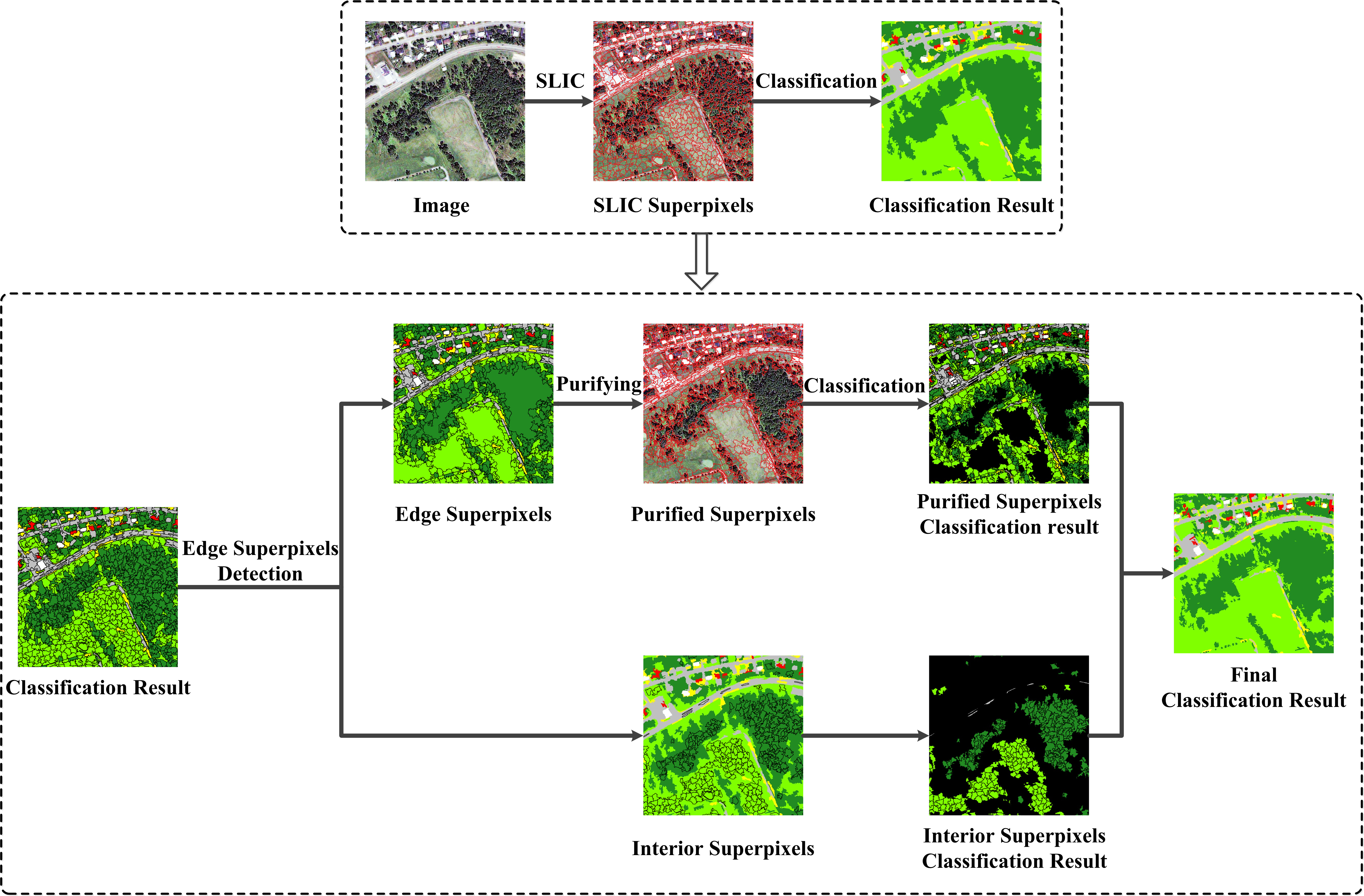
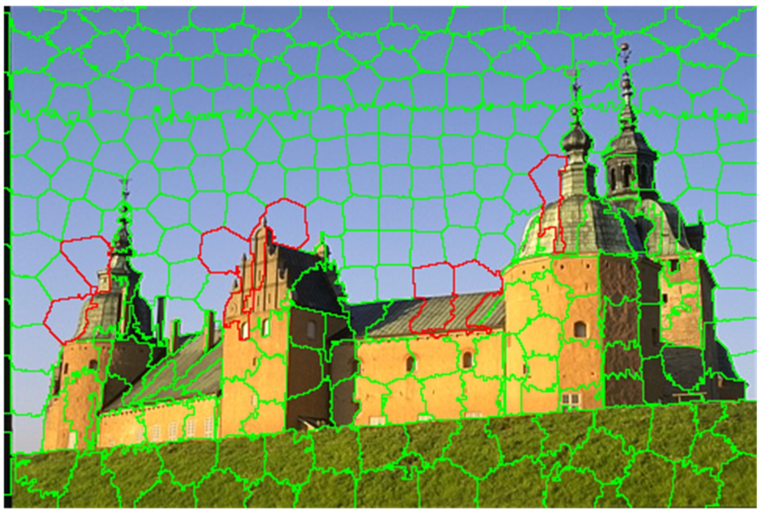
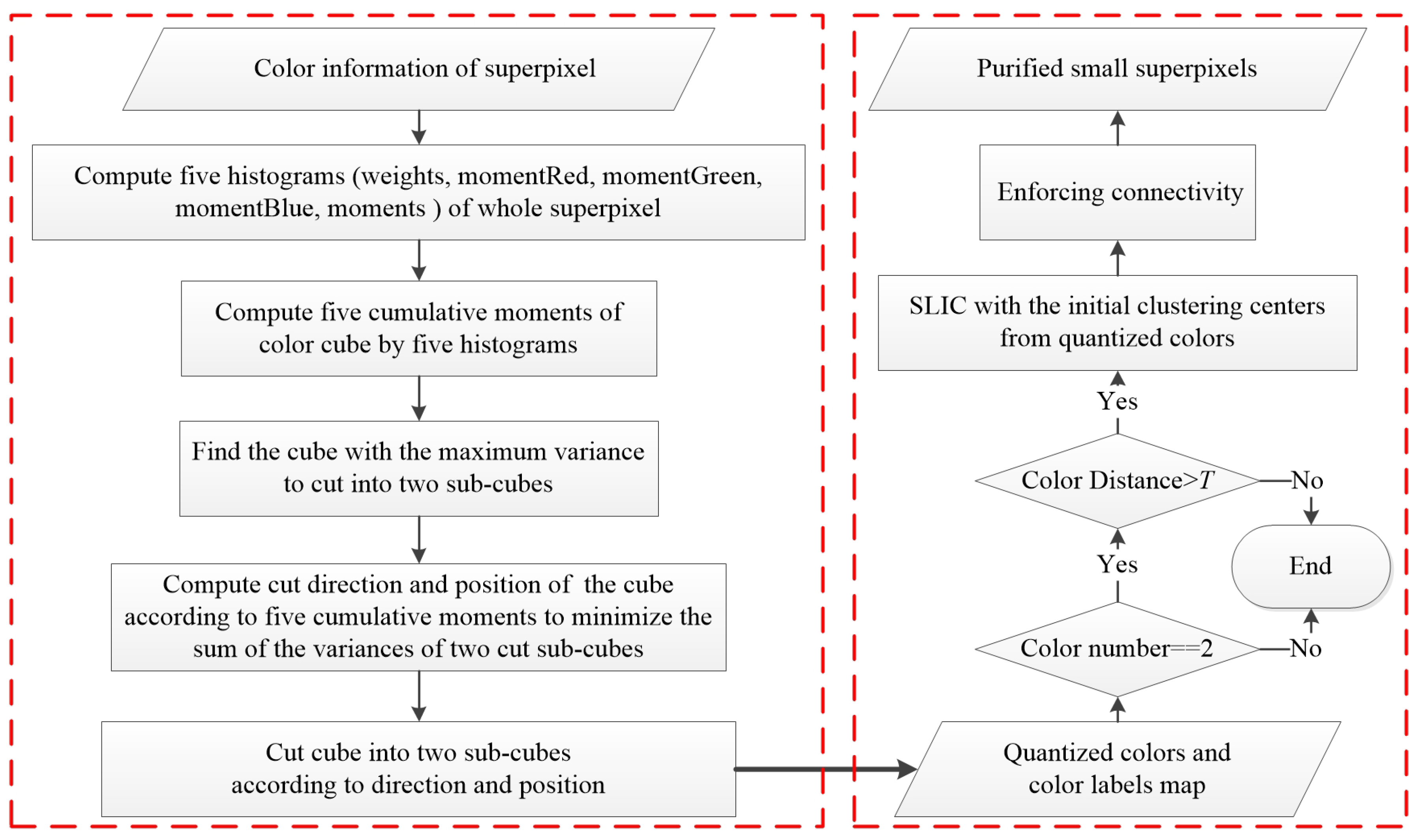
After SLIC, there are some mixed superpixels which contain pixels from different classes. In Figure 1, the superpixels circled in red are mixed superpixels. These mixed superpixels are mainly caused by the improper locations of initial cluster centers in SLIC. If the initial cluster center is near the boundary, a mixed superpixel may be generated because the spatial proximity is taken into consideration in the calculation of distance D. To avoid the error caused by these mixed superpixels in subsequent process, a SLIC superpixels purification algorithm based on color quantization is proposed in this section. It aims at dividing mixed superpixels into pure small superpixels. The procedure of the proposed superpixels purification algorithm is shown in Figure 2.
Color quantization is a process that tries to reduce the number of colors in a given image to a certain limited number given by the external factors, while keeping a visual essence of that image intact [38,39]. I is usually used to satisfy display capabilities of certain devices, to reduce a raw size of the image. The color counts in a source image are usually much higher than those allowed, so the algorithm has to discard the colors carefully. As the Wu’s Color Quantizer [36] can provide very good picture quality unreachable by other algorithms [39], it is selected to quantize the colors in the mixed superpixels. Based on the observation that most mixed superpixels contains two different classes, the number of colors assigned for Wu’s Color Quantizer is 2. It should be noted that in the process of cutting a color cube into two sub-cubes, if the superpixel is pure, the cutting will be ignored. Therefore, in the quantization, if the superpixel is very pure, the number of colors in the output will be changed to be 1 automatically. After quantization, if the superpixel is not pure, the outputs of Wu’s Color Quantizer are two extracted colors and a map with the color labels.
The purifying process is based on the outputs of the color quantization which can detect different colors in the superpixels. There are two conditions in which the superpixels will not be considered as mixed: (1) the superpixel is very pure so that the output of the color quantization algorithm is a single color; and (2) the distance between the two extracted colors is less than the threshold T. These two conditions are shown in two diamond boxes in Figure 2. Assuming that two colors extracted by the color quantization algorithm are and with the color components in CIELab color space, instead of calculating the Euclidean distance, the CIELab color distance between and is calculated with CIEDE2000 Color-Difference Formula [40], which is more precise.
If a superpixel is labeled as mixed, it will be processed by an iterative cluster procedure which is similar to SLIC. First, two cluster centers are generated by calculating the mean vector of all the pixels belonging to the and according to the labeled map generated from color quantization. Then, the distance D between each cluster center and pixels in the superpixels are calculated. According to the calculated distance, each pixel is assigned to the nearest cluster center. Next, new cluster centers are updated by calculating the mean vector of all the pixels belonging to the same cluster center. As same as SLIC, the iterative procedure will stop when the residual error converges or the number of iterations reaches the threshold 10. After enforcing connectivity, more than one new superpixels will be generated. These small superpixels are purer than the original mixed superpixel.
2.3. High Spatial Resolution Remote Sensing Image Classification Based on Purified SLIC Superpixels
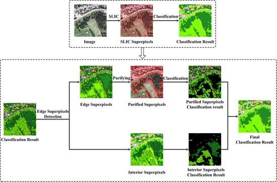
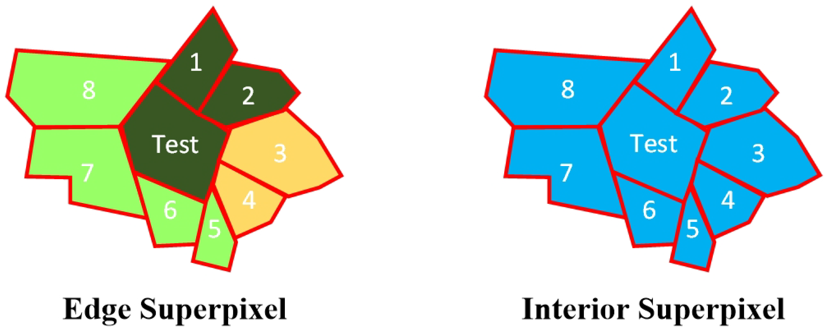
The SLIC superpixels have been used for the classification of high spatial resolution remote sensing image in [1]. However, if the generated superpixels are not pure, the classification result of these superpixels must be incorrect. Therefore, the proposed purified SLIC is applied to the classification for getting better result. As the size of the high spatial resolution remote sensing image is always large, the number of generated SLIC superpixels will also be large. Some interior superpixels in the ground objects do not need to be purified. Therefore, to avoid unnecessary purifying, an efficient method which can detect interior superpixels is needed. Based on the observation that most mixed superpixels locate near the boundaries separating different classes, a mixed superpixels detection scheme utilizing the information of classification result is applied in this section. At first, a classification based on the SLIC superpixels will be executed. In the generated classification map, superpixels are divided into two groups, edge superpixel and interior superpixel (as shown in Figure 3), according to superpixel’s class label and its surrounding neighbor superpixels’ class labels. For the superpixel with the class label , assuming that its neighbor superpixels belong to a set , the group label is defined as follows:
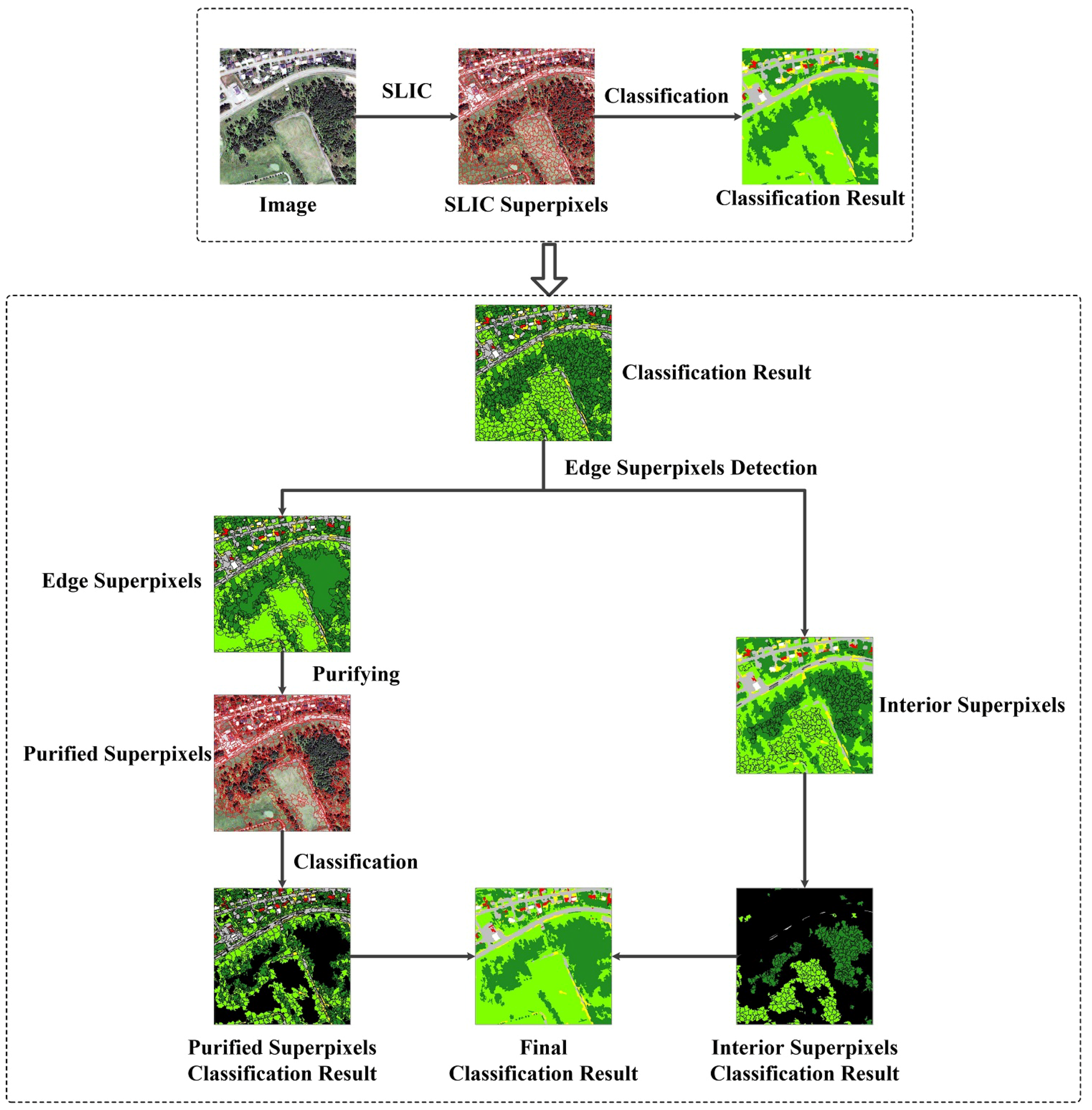
Then, all edge superpixels are the detected candidate mixed superpixels. The purifying process will be executed in these edge superpixels. After purifying, all superpixels generated from edge superpixels will be reclassified. The final classification result is the union result of the interior superpixels and the purified edge superpixels. The outline of the proposed classification scheme is illustrated in Figure 4.
3. Datasets and Experimental Results
3.1. Datasets
The Berkeley Segmentation Dataset 500 [41,42] was the first to be used for superpixel algorithm evaluation. It contains 500 images and provides at least five high-quality ground truth segmentations per image. The images represent simple outdoor scenes, showing landscape, buildings, animals and humans, where foreground and background are usually easily identified. We chose three images with the size of from the BSDS500 to validate the advantages of the proposed purification algorithm. As each image has at least five high-quality ground truth segmentations, we evaluated the generated superpixels on all ground truth segmentations and calculated the mean value for each metric. The image and one of the ground truth segmentations are shown in Figure 5.
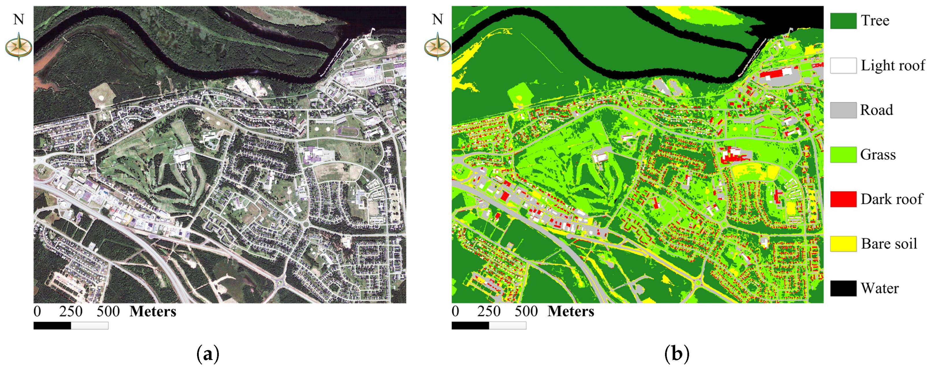
In terms of high spatial resolution remote sensing image, we chose an image with the resolution of 0.5 m obtained from WorldView-2 satellite to validate the performance of the Purified SLIC superpixels. The selected image with the size of pixels covers the residential and forest area of the city Oromocto in Canada. The image contains four bands: red, green, blue and NIR band. The reference map was generated from an object based classification result with seven classes: tree, grass, road, light roof, dark roof, water and bare soil. Then, the label of misclassified regions were modified manually by an independent experienced researcher. The image and the reference map are shown in Figure 6.
3.2. Segmentation Quality Comparison between Purified SLIC Superpixels and Original SLIC Superpixels
We used three metrics [30], namely Boundary Recall (Rec) [43], Under-segmentation Error (UE) [12,15,44], and Explained Variation (EV) [45], to evaluate the performance of the purified SLIC superpixels and original SLIC superpixels. In the following, let and be partitions of the same image and , be an image with being the pixel location and the corresponding intensity or color. The Rec is a commonly used metric to asses boundary adherence given ground truth. Let and be the number of false negative and true positive boundary pixels in S with respect to G. Then, Rec is defined as:
UE measures the “leakage” of superpixels with respect to G and, therefore, implicitly also measures boundary adherence. Here, “leakage” refers to the overlap of superpixels with multiple, nearby ground truth segments. The formulation is computed as:
EV quantifies the quality of a superpixel segmentation without relying on ground truth. As image boundaries tend to exhibit strong change in color and structure, EV assesses boundary adherence independent of human annotations. It is defined as:
where and are the mean color of superpixel and the image I, respectively.
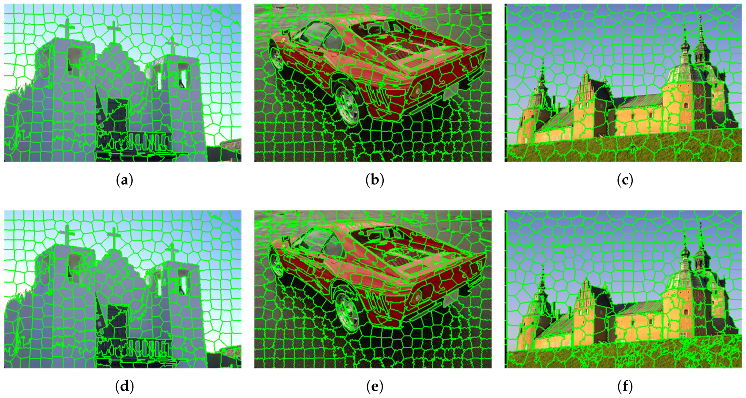
It should be noted that, for generated superpixels, higher Rec and EV are better while lower UE is better. With these metrics, we compared the segmentations of the three initial superpixel sizes , and generated from purified SLIC and original SLIC in the three images selected from BSDS500. The calculated metrics are shown in Table 1. The segmentation maps with the initial superpixel size for three images are shown in Figure 7. As can be observed, the purified SLIC superpixels outperformed the SLIC pixels for all images in terms of all metrics. Moreover, from segmentation maps in Figure 7, it can be seen that obvious mixed SLIC superpixels are divided into pure superpixels by the proposed purification algorithm.
3.3. Comparison of Remote Sensing Image Classification Results Generated from Purified SLIC Superpixels and Original SLIC Superpixels
We used three metrics, namely overall accuracy (OA), average accuracy (AA) and kappa coefficient, to evaluate the performance of classification based on the purified SLIC and original SLIC superpixels in the image of the city Oromocto in Canada. As in [1], we chose the Random Forest (RF) classifier [46] to do the classification. RF classifier builds a set of trees that are created by selecting a subset of training samples through a bagging approach, while the remaining samples are used for an internal cross-validation to estimate how well the RF model performs [47]. The number of trees in the RF that should be assigned by users was set as 500, which had been shown to be sufficient in order to stabilize the errors before reaching this number of classification trees [47]. The object attributes used for classification included: (1) spectral attributes of mean value and standard deviation of each band for each superpixel, brightness, and NDVI; and (2) gray level co-occurrence matrix (GLCM) texture attributes [48] of GLCM standard deviation, GLCM homogeneity and GLCM correlation. The shape attributes were excluded because the superpixel is too small to describe the real shape information of ground object and most superpixels have similar sizes and shapes. As the test image contains four bands, the number of calculated object attributes for each superpixel is 13. In the stage of training, to guarantee the purity of sample superpixels, we filtered the SLIC superpixels with a rule that there must be a class occupying 90% pixels in the superpixel. Then, 50% of the filtered SLIC superpixels were randomly selected as samples and the remaining SLIC superpixels were used to evaluate the performance of the classification. The number of generated superpixels and selected samples with three initial superpixel sizes of , and are listed in Table 2. The color distance threshold T is 6, which is used in the purifying stage to judge whether the edge superpixels should be purified or not. It should be noted that the SLIC superpixels and purified SLIC superpixels were both classified with the same classification model, which was trained from filtered SLIC superpixels. All tests were conducted on a computer with an Intel Core i5-7300HQ CPU (2.50 GHz) processor with 8 GB RAM, using a 64-bit Windows 10 operating system.
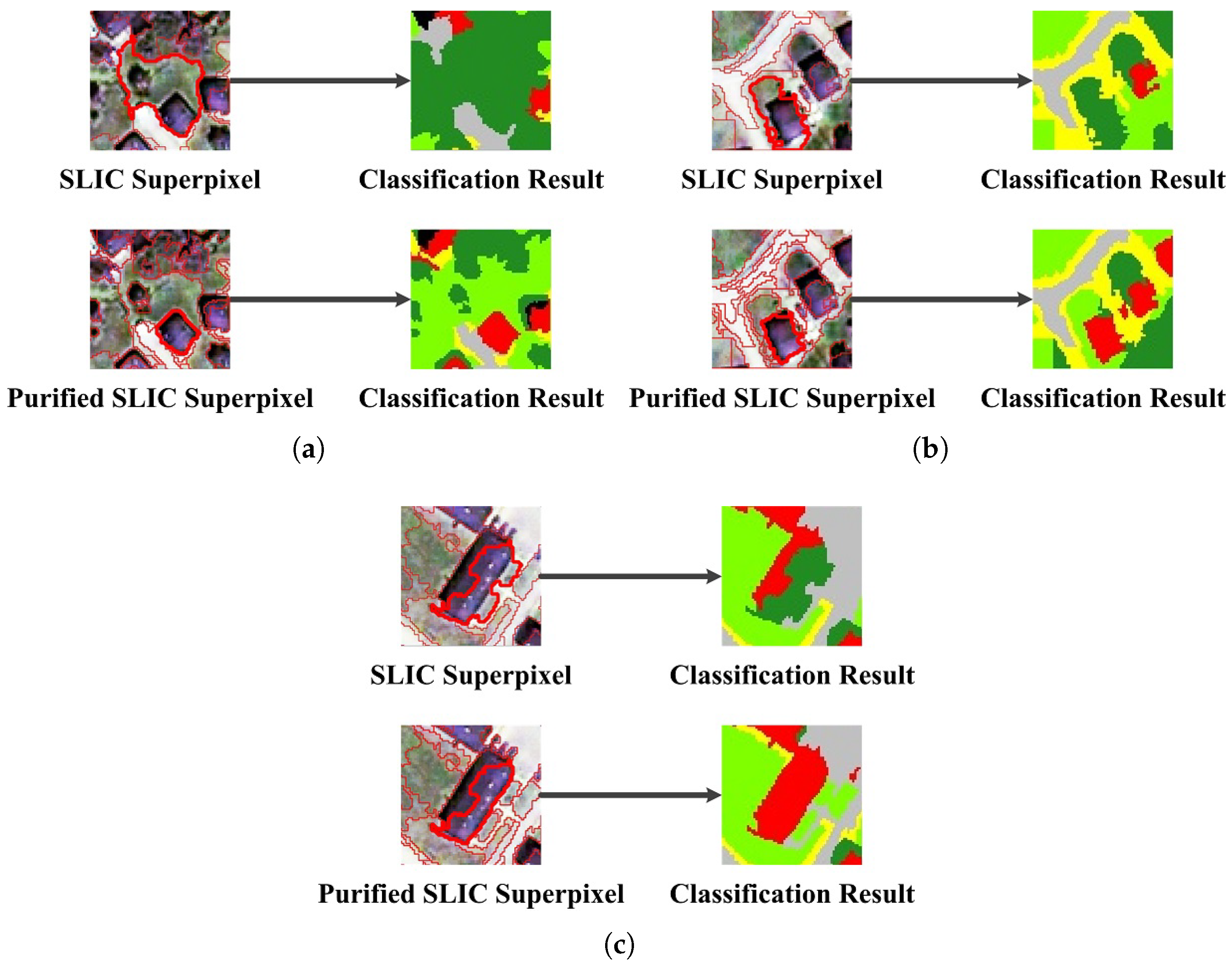
With three evaluation metrics mentioned above, we compared the classification results based on purified SLIC and original SLIC superpixels with different initial superpixel sizes. In addition, to demonstrate that purifying all superpixels is unnecessary, the classification based on the scheme purifying all SLIC superpixels was also investigated. The SLIC superpixels and purified SLIC superpixels generated in a subset image of pixels cut from the test image are shown in Figure 8. The average classification accuracy in ten runs of classification for the whole image are listed in the Table 3. As some superpixels are not pure, the classification accuracy was calculated based on individual pixels within superpixels. The classification maps for one run are shown in Figure 9. As can be observed, the classification based on purified SLIC superpixels outperformed the classification based on SLIC superpixels in all scales. The overall accuracy increases are, respectively, 1.94%, 3.42% and 4.68% for scales to . To better show the performance of the proposed method, we selected some small plots in the image to demonstrate how the proposed purification algorithm optimizes the classification (as shown in Figure 10). For each plot, the SLIC superpixel circled in red is mixed and the related classification is incorrect while the generated purified SLIC superpixel is pure and the related classification is correct. In addition, the accuracy of the scheme purifying all superpixels is a little lower than the proposed scheme purifying edge superpixels because unnecessary purifying for some SLIC superpixels leads to misclassification.
4. Discussion
The comparison of classification accuracy shows that the classification based on purified SLIC superpixels outperformed the classification based on SLIC superpixels. However, from the outline of the proposed classification, it is easy to find that the proposed classification has three additional steps compared to the classification based on SLIC superpixels. It means that the proposed classification will take more time than the classification based on SLIC superpixels. The average time for each step in ten runs of classifications are tabulated in Table 4. With the increase of initial SLIC superpixel size, the time decreases because less SLIC superpixels are generated. We can find that the feature extraction is the most time-consuming step in the classification, occupying more than 90% of the time in classification. Compared with the classification based on SLIC superpixels, the proposed classification generates a lot of new small superpixels so that the features of these new superpixels need to be calculated. Thus, calculating features for new superpixels also costs most time among the three additional steps in the proposed classification. Moreover, the purifying step takes more than four times that of SLIC. As for the total time, the proposed classification costs 2711 s, 2260 s and 1852 s more than the classification based on SLIC superpixels for scales to , respectively. Despite the increased time cost is significant, the improvement in the classification accuracy is encouraging.
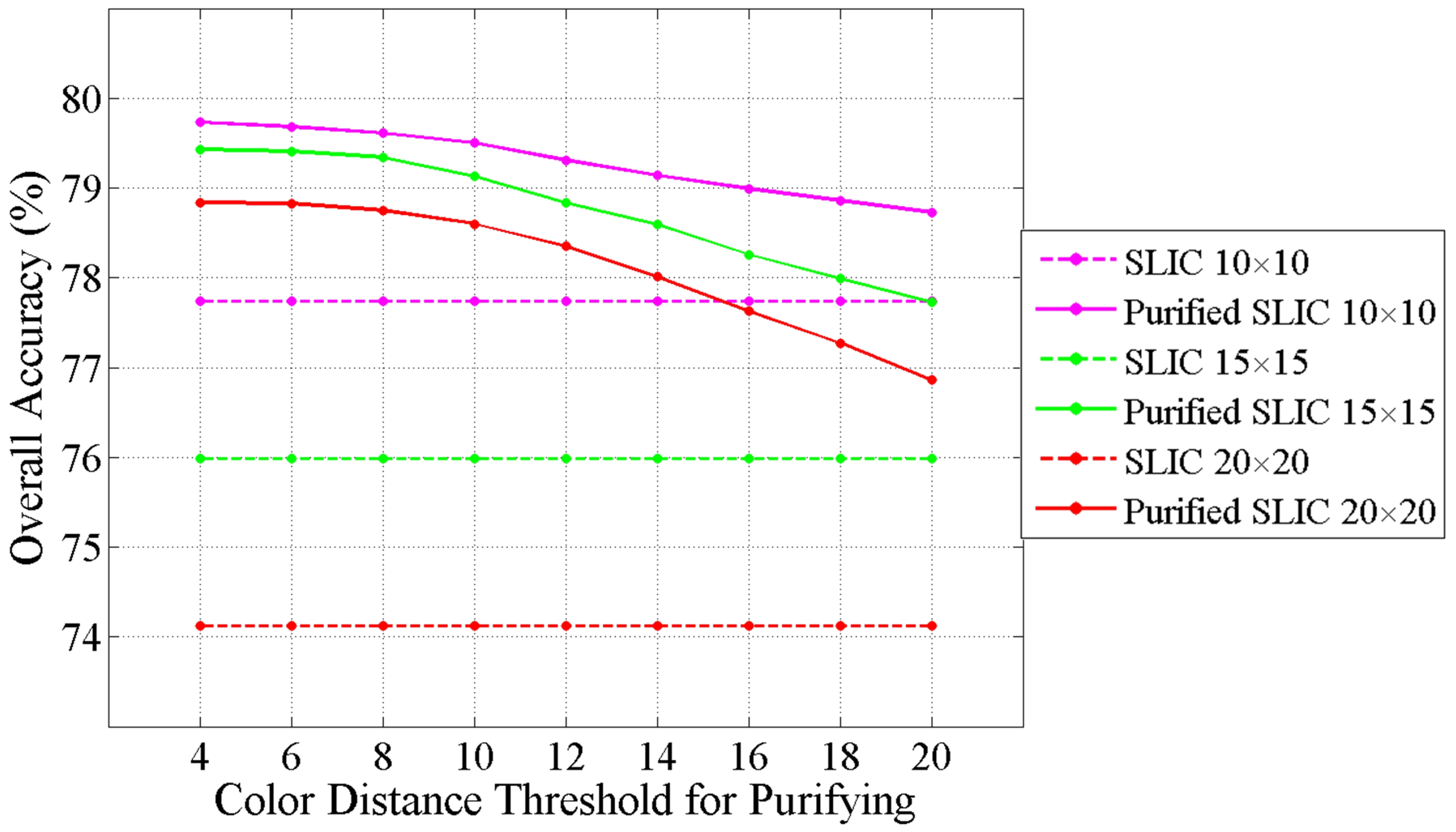
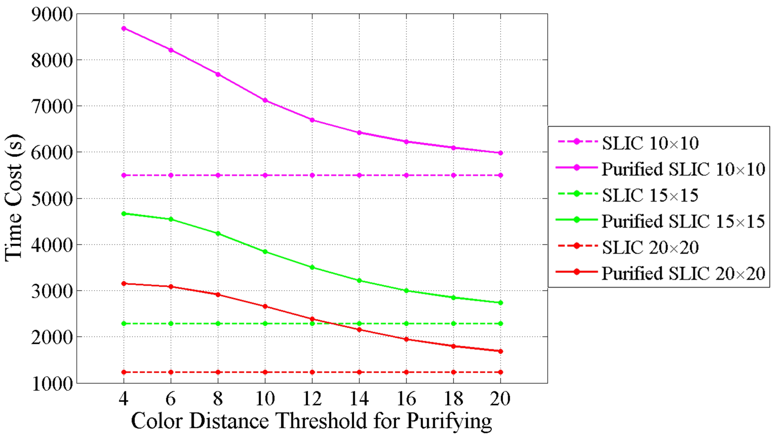
There are two factors that can influence the running time of the classification based on purified SLIC superpixels. The first factor is the complexity of the test image. If the test image contains less boundary between different classes, the number of detected edge superpixels will decrease, thus reducing time cost of subsequent procedure. The second factor is the color distance threshold T used in purifying step. The color distance threshold T determines whether the edge superpixel should be purified or not according to the output of color quantization. If the T is too small, the number of edge superpixels need to be purified is large so that the number of new superpixels generated in purifying is large. Even some superpixels that are interpreted as pure superpixels by human analysis will be purified. The time cost for calculating features of new superpixels will be high. On the contrary, if T is too large, the number of edge superpixels that need to be purified is small so that the number of new superpixels generated in purifying is small. The time cost for calculating features of new superpixels will be low. However, some mixed edge superpixels may not be purified. Therefore, the T not only influences the time cost of the proposed classification, but also affects the accuracy of the classification. To investigate the influence of the color distance threshold T for the proposed classification, we ran the proposed classification with different T, from 4 to 20 with an interval of 2. The classification accuracy and time cost for each T are shown in Figure 11 and Figure 12, respectively. In Figure 11, the OA of the proposed classification continually declines with the increase of T for three scales. However, the OA of the proposed classification is obviously higher than the classification based on SLIC superpixels even with a T of 20, which is large enough for judging that two colors are similar. It means that the color difference in some mixed SLIC superpixels is very explicit. As for the time cost, the line chart in Figure 12 shows that the time cost reduces with the growing of T. When the T reaches 20, the difference of the time cost between the proposed classification and the classification based on SLIC superpixels is below 500 s. As can be concluded, the choice of T is a balance of performance and efficiency, and choosing a T which can improve the performance of subsequent processes is not difficult for users.
Some limitations also exist in the proposed purification algorithm. For example, we fix the number of colors at two for the color quantization process because most mixed superpixels only contain pixels from two different classes. However, a few mixed superpixels containing pixels from more than two different classes are still generated. For these mixed superpixels, the results of color quantization are not accurate, thus the purifying cannot divide the superpixel accurately. The current solution for this problem is to run the purifying process multiple times. For each mixed superpixel, the purifying will not stop unless all generated new superpixels cannot be divided. In this way, the generated new superpixels will be pure no matter how many classes are contained in the original superpixel. Another limitation is that a few superpixels that are identified as pure by human eyes may also be purified. For example, as shown in Figure 7f, some pure grass superpixels on the bottom of the picture are purified to be small superpixels. The reason is that the color variation for these grass superpixels are higher than the assigned color distance threshold. Although most unnecessary purifying does not negatively affect the accuracy of subsequent process, the extra time cost for the purifying will lower the efficiency. Therefore, developing methods to avoid the unnecessary purifying is a good direction for further research. In addition, although the proposed purification algorithm is applied to SLIC superpixels in this paper, it can also be used to purify mixed superpixels generated by other superpixel algorithms.
5. Conclusions
In this paper, a SLIC superpixels purification algorithm based on color quantization is proposed to improve the accuracy of superpixel-based high spatial resolution remote sensing image classification. The novelty of this study consists of two factors: (1) using the quantized color information in the SLIC superpixel to purify mixed superpixels; and (2) applying a classification scheme to avoid purifying superpixels that do not need to be purified. The first factor successfully reduces the misclassification caused by mixed SLIC superpixels. The second factor reduces the unnecessary purifying process and reserves pure superpixels in the original scale. The experiments on images from BSDS500 demonstrate that the purified SLIC superpixels are better than SLIC superpixels in all three metrics for evaluating superpixels. The experiments on the high resolution remote sensing image demonstrate that, compared with the classification based on SLIC superpixels, the classification based on purified SLIC superpixels can achieve the accuracy increase of 1.94%, 3.42% and 4.68% at scale , , and , respectively.
Author Contributions
H.T. and F.T. proposed the model and designed the experiments. H.T. wrote the manuscript. W.Z. implemented the experiments and edited the manuscript. Y.Z. reviewed and edited the manuscript.
Funding
This research was funded by the National Natural Science Foundation of China (41171339 and 61501413).
Acknowledgments
The authors would like to thank the handling editor and anonymous reviewers for their valuable comments and suggestions, which significantly improved the quality of this paper.
Conflicts of Interest
The authors declare no conflict of interest.
References
- Csillik, O. Fast Segmentation and Classification of Very High Resolution Remote Sensing Data Using SLIC Superpixels. Remote Sens. 2017, 9, 243. [Google Scholar] [CrossRef]
- Georganos, S.; Grippa, T.; Vanhuysse, S.; Lennert, M.; Shimoni, M.; Kalogirou, S.; Wolff, E. Less is more: Optimizing classification performance through feature selection in a very-high-resolution remote sensing object-based urban application. GIScience Remote Sens. 2018, 55, 221–242. [Google Scholar] [CrossRef]
- Han, W.; Feng, R.; Wang, L.; Cheng, Y. A semi-supervised generative framework with deep learning features for high-resolution remote sensing image scene classification. ISPRS J. Photogramm. Remote Sens. 2018, 145, 23–43. [Google Scholar]
- Blaschke, T.; Hay, G.J.; Kelly, M.; Lang, S.; Hofmann, P.; Addink, E.; Feitosa, R.Q.; Meer, F.V.D.; Werff, H.V.D.; Coillie, F.V. Geographic Object-Based Image Analysis—Towards a new paradigm. ISPRS J. Photogramm. Remote Sens. 2014, 87, 180–191. [Google Scholar] [CrossRef] [PubMed]
- Hay, G.J.; Castilla, G. Geographic Object-Based Image Analysis (GEOBIA): A new name for a new discipline. In Object-Based Image Analysis; Springer: Berlin/Heidelberg, Germany, 2008; pp. 75–89. [Google Scholar]
- Blaschke, T. Object based image analysis for remote sensing. ISPRS J. Photogramm. Remote Sens. 2010, 65, 2–16. [Google Scholar] [Green Version]
- Cheng, J.; Bo, Y.; Zhu, Y.; Ji, X. A novel method for assessing the segmentation quality of high-spatial resolution remote-sensing images. Int. J. Remote Sens. 2014, 35, 3816–3839. [Google Scholar] [CrossRef]
- Arvor, D.; Durieux, L.; Andrés, S.; Laporte, M.A. Advances in geographic object-based image analysis with ontologies: A review of main contributions and limitations from a remote sensing perspective. ISPRS J. Photogramm. Remote Sens. 2013, 82, 125–137. [Google Scholar] [CrossRef]
- Drăguţ, L.; Csillik, O.; Eisank, C.; Tiede, D. Automated parameterisation for multi-scale image segmentation on multiple layers. ISPRS J. Photogramm. Remote Sens. 2014, 88, 119–127. [Google Scholar] [CrossRef] [PubMed]
- Baatz, M.; Schäpe, A. An optimization approach for high quality multi-scale image segmentation. Angew. Geogr. Inf. Sverarbeitung 2000, 12, 12–23. [Google Scholar]
- Tong, H.; Maxwell, T.; Zhang, Y.; Dey, V. A supervised and fuzzy-based approach to determine optimal multi-resolution image segmentation parameters. Photogramm. Eng. Remote Sens. 2012, 78, 1029–1044. [Google Scholar] [CrossRef]
- Achanta, R.; Shaji, A.; Smith, K.; Lucchi, A.; Fua, P.; Süsstrunk, S. SLIC Superpixels Compared to State-of-the-Art Superpixel Methods. IEEE Trans. Pattern Anal. Mach. Intell. 2012, 34, 2274–2282. [Google Scholar] [CrossRef] [PubMed]
- Zhang, G.; Jia, X.; Hu, J. Superpixel-based graphical model for remote sensing image mapping. IEEE Trans. Geosci. Remote Sens. 2015, 53, 5861–5871. [Google Scholar] [CrossRef]
- Ren, X.; Malik, J. Learning a classification model for segmentation. In Proceedings of the Ninth IEEE International Conference on Computer Vision, Nice, France, 14–17 October 2003; Volume 1, pp. 10–17. [Google Scholar]
- Neubert, P.; Protzel, P. Superpixel benchmark and comparison. In Proceedings of the Forum Bildverarbeitung 2012, Regensburg, Germany, 29–30 November 2012; Volume 6. [Google Scholar]
- Li, Z.; Chen, J. Superpixel segmentation using linear spectral clustering. In Proceedings of the IEEE Conference on Computer Vision and Pattern Recognition, Boston, MA, USA, 7–12 June 2015; pp. 1356–1363. [Google Scholar]
- Shi, C.; Wang, L. Incorporating spatial information in spectral unmixing: A review. Remote Sens. Environ. 2014, 149, 70–87. [Google Scholar] [CrossRef]
- Fourie, C.; Schoepfer, E. Data transformation functions for expanded search spaces in geographic sample supervised segment generation. Remote Sens. 2014, 6, 3791–3821. [Google Scholar] [CrossRef]
- Ma, L.; Du, B.; Chen, H.; Soomro, N.Q. Region-of-interest detection via superpixel-to-pixel saliency analysis for remote sensing image. IEEE Geosci. Remote Sens. Lett. 2016, 13, 1752–1756. [Google Scholar] [CrossRef]
- Arisoy, S.; Kayabol, K. Mixture-based superpixel segmentation and classification of SAR images. IEEE Geosci. Remote Sens. Lett. 2016, 13, 1721–1725. [Google Scholar] [CrossRef]
- Guo, J.; Zhou, X.; Li, J.; Plaza, A.; Prasad, S. Superpixel-based active learning and online feature importance learning for hyperspectral image analysis. IEEE J. Sel. Top. Appl. Earth Obs. Remote Sens. 2017, 10, 347–359. [Google Scholar] [CrossRef]
- Tong, F.; Tong, H.; Jiang, J.; Zhang, Y. Multiscale union regions adaptive sparse representation for hyperspectral image classification. Remote Sens. 2017, 9, 872. [Google Scholar] [CrossRef]
- Li, S.; Lu, T.; Fang, L.; Jia, X.; Benediktsson, J.A. Probabilistic fusion of pixel-level and superpixel-level hyperspectral image classification. IEEE Trans. Geosci. Remote Sens. 2016, 54, 7416–7430. [Google Scholar] [CrossRef]
- Jiang, J.; Ma, J.; Chen, C.; Wang, Z.; Cai, Z.; Wang, L. SuperPCA: A Superpixelwise PCA Approach for Unsupervised Feature Extraction of Hyperspectral Imagery. IEEE Trans. Geosci. Remote Sens. 2018, 56, 4581–4593. [Google Scholar] [CrossRef] [Green Version]
- Jiang, J.; Ma, J.; Wang, Z.; Chen, C.; Liu, X. Hyperspectral Image Classification in the Presence of Noisy Labels. IEEE Trans. Geosci. Remote Sens. 2019, 57, 851–865. [Google Scholar] [CrossRef]
- Ortiz Toro, C.; Gonzalo Martín, C.; García Pedrero, Á.; Menasalvas Ruiz, E. Superpixel-based roughness measure for multispectral satellite image segmentation. Remote Sens. 2015, 7, 14620–14645. [Google Scholar] [CrossRef]
- Vargas, J.E.; Falcão, A.X.; Dos Santos, J.; Esquerdo, J.C.D.M.; Coutinho, A.C.; Antunes, J. Contextual superpixel description for remote sensing image classification. In Proceedings of the 2015 IEEE International Geoscience and Remote Sensing Symposium (IGARSS), Milan, Italy, 26–31 July 2015; IEEE: Piscataway, NJ, USA, 2015; pp. 1132–1135. [Google Scholar]
- Garcia-Pedrero, A.; Gonzalo-Martin, C.; Fonseca-Luengo, D.; Lillo-Saavedra, M. A GEOBIA methodology for fragmented agricultural landscapes. Remote Sens. 2015, 7, 767–787. [Google Scholar] [CrossRef]
- Stefanski, J.; Mack, B.; Waske, B. Optimization of object-based image analysis with random forests for land cover mapping. IEEE J. Sel. Top. Appl. Earth Obs. Remote Sens. 2013, 6, 2492–2504. [Google Scholar] [CrossRef]
- Stutz, D.; Hermans, A.; Leibe, B. Superpixels: An evaluation of the state-of-the-art. Comput. Vis. Image Underst. 2018, 166, 1–27. [Google Scholar] [CrossRef] [Green Version]
- Liu, M.Y.; Tuzel, O.; Ramalingam, S.; Chellappa, R. Entropy rate superpixel segmentation. In Proceedings of the IEEE Conference on Computer Vision and Pattern Recognition, Providence, RI, USA, 20–25 June 2011; pp. 2097–2104. [Google Scholar]
- Conrad, C.; Mertz, M.; Mester, R. Contour-Relaxed Superpixels. In Energy Minimization Methods in Computer Vision and Pattern Recognition; Heyden, A., Kahl, F., Olsson, C., Oskarsson, M., Tai, X.C., Eds.; Springer: Berlin/Heidelberg, Germany, 2013; pp. 280–293. [Google Scholar]
- Buyssens, P.; Gardin, I.; Ruan, S. Eikonal based region growing for superpixels generation: Application to semi-supervised real time organ segmentation in CT images. Innovat. Res. BioMed. Eng. 2014, 35, 20–26. [Google Scholar] [CrossRef] [Green Version]
- Van den Bergh, M.; Boix, X.; Roig, G.; Van Gool, L. SEEDS: Superpixels Extracted Via Energy-Driven Sampling. Int. J. Comput. Vis. 2015, 111, 298–314. [Google Scholar] [CrossRef]
- Yao, J.; Boben, M.; Fidler, S.; Urtasun, R. Real-Time Coarse-to-Fine Topologically Preserving Segmentation. In Proceedings of the IEEE Conference on Computer Vision and Pattern Recognition (CVPR), Boston, MA, USA, 7–12 June 2015. [Google Scholar]
- Wu, X. Color quantization by dynamic programming and principal analysis. ACM Trans. Graph. 1992, 11, 348–372. [Google Scholar] [CrossRef]
- Connolly, C.; Fleiss, T. A study of efficiency and accuracy in the transformation from RGB to CIELAB color space. IEEE Trans. Image Process. 1997, 6, 1046–1048. [Google Scholar] [CrossRef] [PubMed]
- Braquelaire, J.P.; Brun, L. Comparison and optimization of methods of color image quantization. IEEE Trans. Image Process. 1997, 6, 1048–1052. [Google Scholar] [CrossRef] [PubMed] [Green Version]
- K8, S. A Simple—Yet Quite Powerful—Palette Quantizer in C#. Available online: https://www.codeproject.com/Articles/66341/A-Simple-Yet-Quite-Powerful-Palette-Quantizer-in-C (accessed on 25 April 2019).
- Luo, M.R.; Cui, G.H.; Rigg, B. The development of the CIE 2000 colour-difference formula: CIEDE2000. Color Res. Appl. 2001, 26, 340–350. [Google Scholar] [CrossRef]
- Martin, D.; Fowlkes, C.; Tal, D.; Malik, J. A database of human segmented natural images and its application to evaluating segmentation algorithms and measuring ecological statistics. In Proceedings of the Eighth IEEE International Conference on Computer Vision, ICCV 2001, Vancouver, BC, Canada, 7–14 July 2001; Volume 2, pp. 416–423. [Google Scholar]
- Arbelaez, P.; Maire, M.; Fowlkes, C.; Malik, J. Contour Detection and Hierarchical Image Segmentation. IEEE Trans. Pattern Anal. Mach. Intell. 2011, 33, 898–916. [Google Scholar] [CrossRef] [PubMed]
- Martin, D.R.; Fowlkes, C.C.; Malik, J. Learning to detect natural image boundaries using local brightness, color, and texture cues. IEEE Trans. Pattern Anal. Mach. Intell. 2004, 26, 530–549. [Google Scholar] [CrossRef] [PubMed]
- Alex, L.; Adrian, S.; Kutulakos, K.N.; Fleet, D.J.; Dickinson, S.J.; Kaleem, S. TurboPixels: Fast superpixels using geometric flows. IEEE Trans. Pattern Anal. Mach. Intell. 2009, 31, 2290–2297. [Google Scholar]
- Moore, A.P.; Prince, S.J.; Warrell, J.; Mohammed, U.; Jones, G. Superpixel lattices. In Proceedings of the 2008 IEEE conference on computer vision and pattern recognition, Anchorage, AK, USA, 24–26 June 2008; Citeseer: Pittsburgh, PA, USA, 2008; pp. 1–8. [Google Scholar]
- Breiman, L. Random Forests. Mach. Learn. 2001, 45, 5–32. [Google Scholar] [CrossRef] [Green Version]
- Belgiu, M.; Drăguţ, L. Random forest in remote sensing: A review of applications and future directions. ISPRS J. Photogramm. Remote Sens. 2016, 114, 24–31. [Google Scholar] [CrossRef]
- Haralick, R.M.; Shanmugam, K.; Dinstein, I. Textural Features for Image Classification. IEEE Trans. Syst. Man Cybern. 1973, SMC-3, 610–621. [Google Scholar] [CrossRef] [Green Version]
Figure 1.
Mixed superpixels marked by red outline.

Figure 2.
Procedure of the superpixels purification algorithm based on color quantization.

Figure 3.
Edge superpixel and interior superpixel surrounded by neighbor superpixels (different colors represent different labels): (1) edge superpixel is the Test superpixel with green color surrounded by superpixels with different colors; and (2) interior superpixel is the Test superpixel with blue color surrounded by superpixels with same colors.

Figure 4.
Outline of the proposed Classification scheme.

Figure 5.
Images and ground truth segmentations from BSDS500: (a) Image 24,063; (b) Image 29,030; (c) Image 201,080; (d) ground truth of Images 24,063; (e) ground truth of Images 29,030; and (f) ground truth of Images 201,080.
Figure 5.
Images and ground truth segmentations from BSDS500: (a) Image 24,063; (b) Image 29,030; (c) Image 201,080; (d) ground truth of Images 24,063; (e) ground truth of Images 29,030; and (f) ground truth of Images 201,080.

Figure 6.
The selected test image and corresponding reference map: (a) high spatial resolution test image; and (b) reference map.
Figure 6.
The selected test image and corresponding reference map: (a) high spatial resolution test image; and (b) reference map.

Figure 7.
Superpixels generated from SLIC and Purified SLIC with the initial superpixel size : (a) SLIC superpixels for Image 24,063; (b) SLIC superpixels for Image 29,030; (c) SLIC superpixels for Image 201,080; (d) Purified SLIC superpixels for Image 24,063; (e) Purified SLIC superpixels for Image 29,030; and (f) Purified SLIC superpixels for Image 201,080.

Figure 8.
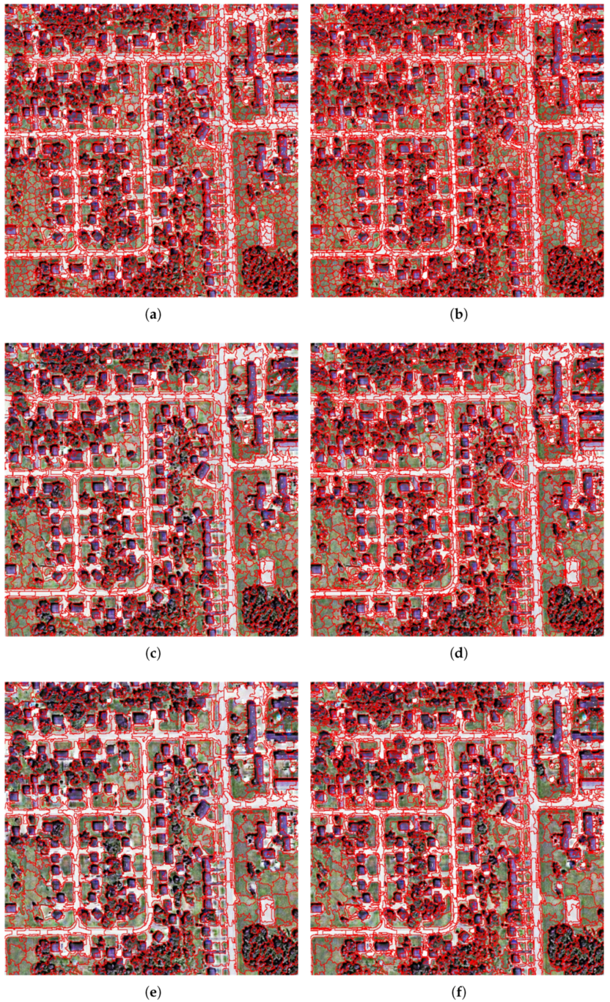
Segmentation maps in three scales: (a) SLIC superpixels; (b) Purified SLIC superpixels; (c) SLIC superpixels; (d) Purified SLIC superpixels; (e) SLIC superpixels; and (f) Purified SLIC superpixels.
Figure 8.
Segmentation maps in three scales: (a) SLIC superpixels; (b) Purified SLIC superpixels; (c) SLIC superpixels; (d) Purified SLIC superpixels; (e) SLIC superpixels; and (f) Purified SLIC superpixels.

Figure 9.
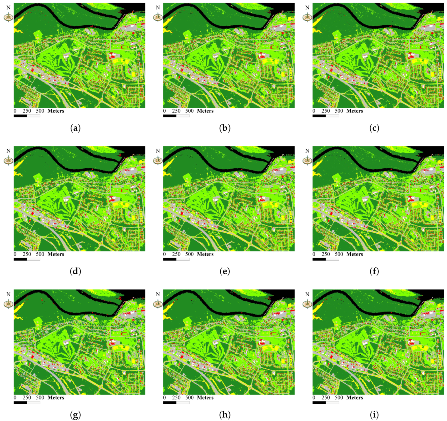
Classification maps based on different superpixels in three scales: (a) SLIC superpixels; (b) Purified SLIC superpixels; (c) Purified all SLIC superpixels; (d) SLIC superpixels; (e) Purified SLIC superpixels; (f) Purified all SLIC superpixels; (g) SLIC superpixels; (h) Purified SLIC superpixels; and (i) Purified all SLIC superpixels.
Figure 9.
Classification maps based on different superpixels in three scales: (a) SLIC superpixels; (b) Purified SLIC superpixels; (c) Purified all SLIC superpixels; (d) SLIC superpixels; (e) Purified SLIC superpixels; (f) Purified all SLIC superpixels; (g) SLIC superpixels; (h) Purified SLIC superpixels; and (i) Purified all SLIC superpixels.

Figure 10.
The detail segmentation maps and classification maps of three plots in which obvious mixed SLIC superpixels are purified.
Figure 10.
The detail segmentation maps and classification maps of three plots in which obvious mixed SLIC superpixels are purified.

Figure 11.
The influence of the color distance threshold T for classification accuracy.

Figure 12.
The influence of the color distance threshold T for time cost.


Table 1.
Evaluation metrics for superpixels.
| Image 24,063 | Image 29,030 | Image 201,080 | |||||||
|---|---|---|---|---|---|---|---|---|---|
| Rec | UE | EV | Rec | UE | EV | Rec | UE | EV | |
| SLIC | 0.8347 | 0.0466 | 0.9736 | 0.8261 | 0.0600 | 0.9170 | 0.8753 | 0.0514 | 0.9268 |
| Purified SLIC | 0.8727 | 0.0360 | 0.9865 | 0.8622 | 0.0434 | 0.9453 | 0.9150 | 0.0328 | 0.9583 |
| SLIC | 0.7743 | 0.0641 | 0.9620 | 0.7840 | 0.0847 | 0.8821 | 0.8391 | 0.0728 | 0.9049 |
| Purified SLIC | 0.8338 | 0.0435 | 0.9834 | 0.8208 | 0.0579 | 0.9342 | 0.9030 | 0.0406 | 0.9507 |
| SLIC | 0.7630 | 0.0776 | 0.9540 | 0.5790 | 0.1051 | 0.8737 | 0.7328 | 0.0937 | 0.8859 |
| Purified SLIC | 0.8202 | 0.0527 | 0.9787 | 0.6523 | 0.0706 | 0.9308 | 0.7883 | 0.0479 | 0.9422 |
Table 2.
Number of SLIC superpixels and selected samples for three scales.
| Tree | 40,621 | 15,555 | 7457 |
| Light Roof | 564 | 189 | 90 |
| Road | 8394 | 3271 | 1614 |
| Grass | 16,651 | 6108 | 2879 |
| Dark Roof | 2069 | 715 | 374 |
| Bare Soil | 4212 | 1483 | 677 |
| Water | 4654 | 1919 | 998 |
| Total | 77,165 | 29,240 | 14,089 |
| SLIC superpixels | 205,700 | 87,442 | 46,778 |
Table 3.
Average classification accuracy in ten runs of classification.
| OA(%) | AA(%) | Kappa | |
|---|---|---|---|
| SLIC | 77.74 | 67.97 | 0.697 |
| Purified SLIC | 79.68 | 71.29 | 0.725 |
| All Purified SLIC | 79.51 | 71.26 | 0.722 |
| SLIC | 75.99 | 65.15 | 0.674 |
| Purified SLIC | 79.41 | 70.83 | 0.722 |
| All Purified SLIC | 79.20 | 70.80 | 0.720 |
| SLIC | 74.12 | 62.80 | 0.648 |
| Purified SLIC | 78.80 | 70.46 | 0.714 |
| All Purified SLIC | 78.62 | 70.42 | 0.712 |
Table 4.
Average time cost (s) for each step in ten runs of classification.
| SLIC | Purified SLIC | SLIC | Purified SLIC | SLIC | Purified SLIC | |
|---|---|---|---|---|---|---|
| SLIC | 27 | 27 | 23 | 23 | 22 | 22 |
| Feature Extraction | 5230 | 5230 | 2177 | 2177 | 1174 | 1174 |
| RF Training | 212 | 212 | 74 | 74 | 33 | 33 |
| Classification | 30 | 30 | 11 | 11 | 5 | 5 |
| Purifying | – | 110 | – | 93 | – | 92 |
| Feature Extraction | – | 2584 | – | 2155 | – | 1752 |
| Classification | – | 17 | – | 12 | – | 8 |
| Total | 5499 | 8210 | 2285 | 4545 | 1234 | 3086 |
© 2019 by the authors. Licensee MDPI, Basel, Switzerland. This article is an open access article distributed under the terms and conditions of the Creative Commons Attribution (CC BY) license (http://creativecommons.org/licenses/by/4.0/).
Share and Cite
MDPI and ACS Style
Tong, H.; Tong, F.; Zhou, W.; Zhang, Y. Purifying SLIC Superpixels to Optimize Superpixel-Based Classification of High Spatial Resolution Remote Sensing Image. Remote Sens. 2019, 11, 2627. https://doi.org/10.3390/rs11222627
AMA Style
Tong H, Tong F, Zhou W, Zhang Y. Purifying SLIC Superpixels to Optimize Superpixel-Based Classification of High Spatial Resolution Remote Sensing Image. Remote Sensing. 2019; 11(22):2627. https://doi.org/10.3390/rs11222627
Chicago/Turabian StyleTong, Hengjian, Fei Tong, Wei Zhou, and Yun Zhang. 2019. "Purifying SLIC Superpixels to Optimize Superpixel-Based Classification of High Spatial Resolution Remote Sensing Image" Remote Sensing 11, no. 22: 2627. https://doi.org/10.3390/rs11222627
Note that from the first issue of 2016, this journal uses article numbers instead of page numbers. See further details here.