Comparison of Five Spatio-Temporal Satellite Image Fusion Models over Landscapes with Various Spatial Heterogeneity and Temporal Variation

Abstract

In recent years, many spatial and temporal satellite image fusion (STIF) methods have been developed to solve the problems of trade-off between spatial and temporal resolution of satellite sensors. This study, for the first time, conducted both scene-level and local-level comparison of five state-of-art STIF methods from four categories over landscapes with various spatial heterogeneity and temporal variation. The five STIF methods include the spatial and temporal adaptive reflectance fusion model (STARFM) and Fit-FC model from the weight function-based category, an unmixing-based data fusion (UBDF) method from the unmixing-based category, the one-pair learning method from the learning-based category, and the Flexible Spatiotemporal DAta Fusion (FSDAF) method from hybrid category. The relationship between the performances of the STIF methods and scene-level and local-level landscape heterogeneity index (LHI) and temporal variation index (TVI) were analyzed. Our results showed that (1) the FSDAF model was most robust regardless of variations in LHI and TVI at both scene level and local level, while it was less computationally efficient than the other models except for one-pair learning; (2) Fit-FC had the highest computing efficiency. It was accurate in predicting reflectance but less accurate than FSDAF and one-pair learning in capturing image structures; (3) One-pair learning had advantages in prediction of large-area land cover change with the capability of preserving image structures. However, it was the least computational efficient model; (4) STARFM was good at predicting phenological change, while it was not suitable for applications of land cover type change; (5) UBDF is not recommended for cases with strong temporal changes or abrupt changes. These findings could provide guidelines for users to select appropriate STIF method for their own applications.

1. Introduction

High spatial resolution (hereafter referred to as “high-resolution”) images with a short revisit cycle are of great significance for various remote sensing applications such as vegetation phenology monitoring [1], forest disturbance mapping [2], and land surface temperature monitoring [3]. However, trade-offs between spatial and temporal resolution always exist in satellite sensor design, which constrain the applications of satellite observations from single satellite sensors. Typical examples include Landsat Thematic Mapper (TM), Enhanced TM plus (ETM+), Operational Land Imager (OLI) imagery with a 30m spatial resolution but a 16-day revisit cycle, and MODerate-resolution Imaging Spectroradiometer (MODIS) imagery with a sub-day revisit cycle but 250/500/1000 m spatial resolutions. To overcome this constraint, many spatial and temporal satellite image fusion (STIF) approaches have been developed [4]. These approaches fuse satellite imagery from one sensor with high spatial but low temporal resolutions (e.g., Landsat imagery) with imagery from the other sensor with high temporal but low spatial resolutions (e.g., MODIS imagery), and generate synthetic imagery with both high spatial and high temporal resolutions. For example, given a pair of Landsat/MODIS images acquired on the same or close date (t₁) and a MODIS image acquired on the other date (t₂), the approaches predict an image with the same spatial resolution of Landsat at t₂, also called a Landsat-like image. The synthetic imagery allows construction of high-quality high-frequency time series data, which promotes the applications of remote sensing in identifying high-frequency change in heterogeneous landscapes.

The existing STIF approaches can be categorized into five groups: weight function-based, unmixing-based, learning-based, Bayesian-based and hybrid methods [5,6,7,8]. The weight function-based methods combine the information of all input images based on a weighting function to predict the pixel values of a high spatial resolution image. The earliest STIF model, i.e., the Spatial and Temporal Adaptive Reflectance Fusion Model (STARFM), is a weight function-based method. STARFM assumes that changes in pure pixels of coarse resolution images, which have only one land cover type within a pixel, can be added to the pixels of fine resolution images for prediction. To deal with a mixed pixel problem, a higher weight is given to purer coarse pixels for prediction. To enhance the performance of STARFM for forest disturbance mapping, Hilker et al. proposed a Spatial Temporal Adaptive Algorithm for mapping Reflectance Change (STAARCH) [2] to detect the temporal changes from MODIS images, considering the landcover type changes and disturbance events that are not recorded in at least one Landsat image. STARFM was also extended for reflectance prediction in heterogeneous regions based on an enhanced STARFM (ESTARFM) method [9], which assumes the change rates of each class are stable in a period and introduces a conversion coefficient in the prediction. Except for the above two methods, many other methods based on STARFM have also been proposed in recent years [6,10,11,12,13,14].

Unmixing-based methods are developed based on linear spectral mixing theory. They estimate the values of high-resolution image pixels by unmixing the low-resolution image pixels. Different from the weight function-based methods, which require both high- and low-resolution images at each band, the unmixing-based methods only require a thematic map that can be derived from the high-resolution image or land-use database [15,16,17,18]. The multi-sensor multiresolution technique (MMT) [19] was the first unmixing technique introduced for spatiotemporal image fusion. MMT was later improved and utilized in many other unmixing-based STIF processes [16,18,20,21,22]. For example, Zurita-Milla et al. designed an Unmixing-Based Data Fusion (UBDF) that introduced constraints into the unmixing process to produce the synthetic images [18]. Amorós-López et al. incorporated a regularized term in the cost function to solve collinearity between endmembers, resulting in better predictions [16].

Learning-based STIF methods are relatively new but developing rapidly. They utilize the relationships between high- and low-resolution image pairs modelled by machine learning algorithms in order to predict an unobserved high-resolution image. Machine learning algorithms used in STIF methods include sparse representation [8,23], artificial neural networks [24], extreme learning [25], and deep learning [26,27,28]. SParse-representation-based SpatioTemporal reflectance Fusion Model (SPSTFM) [23] was the first model that introduced dictionary-pair learning based on two pairs of low- and high-resolution images. To deal with situations where only one high- and low-resolution image pair was available, Song and Huang designed the one-pair learning model [8]. Recently, more attention has been paid to deep convolutional neural networks (CNNs) for spatiotemporal data fusion [28].

Hybrid STIF methods combine procedures from the above two or three categories. The Flexible Spatiotemporal DAta Fusion (FSDAF) [7] model integrates ideas from the unmixing method, weight function-based method and the thin plate spline interpolator. Regularized spatial Unmixing (RspatialU) [29] and Spatial and Temporal Reflectance Unmixing Model (STRUM) [15] also combine the unmixing and weight-function-based methods. Hierarchical Spatiotemporal Adaptive Fusion Model (HSTAFM) [30] integrates a sparse representation within a STARFM-like framework, and the Robust Adaptive Spatial and Temporal Fusion Model (RASTFM) [5] incorporates weight average and super-resolution modules.

Although a large number of STIF methods have been proposed in recent years, their utility has not been quantitatively evaluated. While comparisons are made when a new method is presented, those studies primarily focus on the advantages of the new method or provide an assessment based on only one or two image scenes. Likewise, the existing comparison studies generally assessed two or more STIF methods of no more than two categories [31,32,33]. Emelyanova et al. assessed the accuracies of STARFM and ESTARFM and two simple benchmarking algorithms [31]. Zhang et al. [33] analyzed the capabilities of STARFM and ESTARFM for generating synthetic flooding images. Chen et al. [32] compared three weight function-based methods (STARFM, ESTARFM and ISTARFM) and one learning-based method (SPSTFM). In addition, most existing studies have evaluated model performances using global accuracy indices such as the correlation coefficient (CC), root-mean-square error (RMSE), average absolute difference (AAD) over the whole study areas, while their performances in maintaining pixel-level spatial details were not fully investigated [4]. How sensitive these methods perform in landscapes with different spatial heterogeneity and temporal variations remains unknown.

This study aims to fill this gap by comparing five state-of-art STIF methods from the weight function-based, unmixing-based, learning-based and hybrid categories, and analyzing their sensitivities to spatial heterogeneity and temporal variation both at scene scale and local scale. We did not consider Bayesian-based methods, because the existing methods were either developed for specific applications or had more strict requirements on the input base pair images. Examples include the Bayesian Maximum Entropy method developed for sea surface temperature downscaling [34], the unified fusion method for spatial, temporal and spectral fusion [35], NDVI-BSFM method for NDVI reconstruction [36], and the STBDF method that were implemented using two or three base image pairs [37].

The five models are STARFM, UBDF, one-pair learning, FSDAF, and Fit-FC. Selection of these models was based on the following four considerations: (1) Each model is representative of one of the four categories. Both STARFM and Fit-FC belong to weight function-based methods; STARFM is the most widely used and Fit-FC was recently proposed [4,31]. UBDF, one-pair learning and FSDAF are classical unmixing-based, learning-based and hybrid methods, respectively. (2) All models require only one prior image pair and they do not need ancillary land cover data. It is much easier to meet the input requirements of these methods compared to the STIF methods requiring two or more image pairs, such as ESTARFM. Due to the influence of cloud contamination, scan-line corrector failure of Landsat 7 ETM+ or time inconsistency of image acquisitions, in many applications only one prior image pair is available [5,7,8]. In addition, more high- and low- image pairs as input did not always ensure higher prediction accuracy [32,38]. (3) Availability of the source code. We would thank the authors who provided us with the source codes. (4) We chose the most-cited STIF method with minimal input pair in each category. Related literature citations can be found in Figure 4 in the review article of Zhu et al. [4]. Please note that the Fit-FC method was not included in the figure because this method was published afterwards. Fit-FC is easy to implement and achieves relatively good results, especially when strong temporal change occurs. Although a filter-based model (STARFM) has been included, Fit-FC is still selected as a comparative model.

Landscape spatial heterogeneity and temporal change are the two major factors affecting performances of STIF models [2,6,9,39]. Spatial heterogeneity can be defined as the complexity and variability of a system property in space [40]. In heterogeneous landscapes such as patchy and fragmented crop fields, the sizes of land surface objects can be much smaller than that of a coarse pixel. It is difficult to restore the spectral change of the objects especially when they show different patterns of change. Strong temporal change, such as change in land cover type, during the fusion period is also a tough scenario for STIF models [6]. Delineating the boundary of change is extremely difficult, because the information on boundary change is not represented in the available fine image, and the boundary of objects is usually not visible in any of the coarse images. As the available fine images at t₁ may be very different from the ideal prediction at t₂, making full use of the available fine image is a critical issue. In existing STIF studies, the assessment of heterogeneity or temporal change has mainly been conducted through subjective evaluations [6,9]. In this manuscript, we aim to quantitatively analyze the spatial heterogeneity and temporal changes of landscapes, assess their impacts on the performances of the five STIF methods, and discuss the possible reasons. Suggestions will be given to help users select the suitable model for their studies.

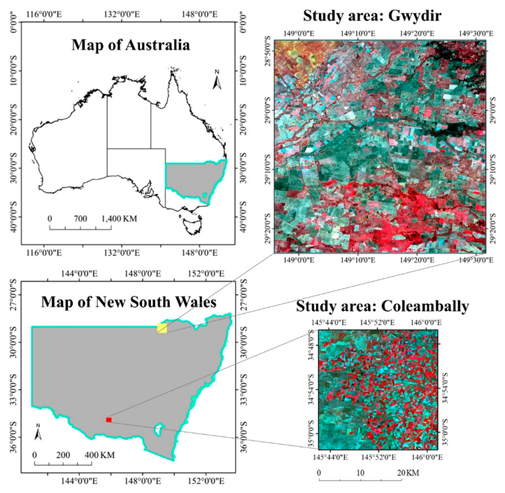
2. Study Area and Datasets

The dataset tested in this research was released by Emelyanova et al. [31] and has been widely used in other studies [5,7,28,41]. This dataset contains a total of 31 time series Landsat and MODIS image pairs over two study sites with contrasting spatial and temporal variability (Figure 1). The Coleambally Irrigation Area (hereafter referred to as ‘Coleambally’) is located in southern New South Wales and the temporal dynamics of surface reflectance is mainly associated with crop phenology in small patchy fields. For Coleambally, seventeen Landsat 7 ETM+-MODIS pairs were available during the austral summer growing season from October 2001 to May 2002 (

Table 1. Landsat and MODIS image pairs for Coleambally and Gwydir sites.

Coleambally		Gwydir
Image No.	Date	Image No.	Date
1	08 October 2001	1	16 April 2004
2	17 October 2001	2	02 May 2004
3	02 November 2001	3	05 July 2004
4	09 November 2001	4	06 August 2004
5	25 November 2001	5	22 August 2004
6	04 December 2001	6	25 October 2004
7	05 January 2002	7	26 November 2004
8	12 January 2002	8	12 December 2004
9	13 Feberary 2002	9	28 December 2004
10	22 Feberary 2002	10	13 January 2005
11	10 March 2002	11	29 January 2005
12	17 March 2002	12	14 Feberary 2005
13	02 April 2002	13	02 March 2005
14	11 April 2002	14	03 April 2005
15	18 April 2002
16	27 April 2002
17	04 May 2002

). The Lower Gwydir Catchment (hereafter referred to as ‘Gwydir’) is located in northern New South Wales, where fourteen Landsat 5 TM-MODIS pairs were available from April 2004 to April 2005. A large flood occurred in mid-December 2004 (image #8 in Table 1), leading to inundation over large areas. Different from the Coleambally site, the spectral change in Gwydir site was mainly caused by land cover type change from vegetation to flood water, and thus Gwydir was considered a more temporally dynamic site. All the satellite images had been atmospherically corrected [31] and were downloaded from http://dx.doi.org/10.4225/08/5111AC0BF1229 and http://dx.doi.org/10.4225/08/5111AD2B7FEE6 (Accessed on 15 October 2018). The spatial resolutions for the geometrically corrected Landsat and MODIS images are 25 m and 500 m, respectively. Before applying the STIF methods (except for Fit-FC model), MODIS images were resampled to 25 m resolution using a nearest neighbor algorithm to match the Landsat data resolution [7,8,42].

3. Methods

3.1. Five STIF Models

3.1.1. STARFM

STARFM [42] was developed based on the assumption that both fine- and coarse-resolution pixels have consistent spectral change from t₁ to t₂ if the coarse pixel is homogeneous. For this ideal situation, the spectral change of coarse pixels from t₁ to t₂ can be directly added to the fine pixel at t₁. However, if the coarse pixel contains mixed land cover types considered at the fine resolution, the fine pixel at t₂ is predicted from neighboring similar pixels within a moving window based on a weighted sum function. Similar pixels are selected using a thresholding pre-classification method. Higher weights are given to those pixels with shorter spectral, temporal, and spatial distances. Finally, the central Landsat pixel on t₂ is calculated by the corresponding MODIS pixels together with Landsat pixels through the proposed weight function. The algorithm is characterized in Equation (1),

$$L(x_{\frac{\omega }{2}},y_{\frac{\omega }{2}},t_0)={\displaystyle \sum _{i=1}^{\omega }{\displaystyle \sum _{j=1}^{\omega }{\displaystyle \sum _{k=1}^n{W}_{ijk}(M(x_i,y_j,t_0)+L(x_i,y_j,t_k)-M(x_i,y_j,t_k))}}},$$

(1)

where L(x_ω/2, y_ω/2, t₀) is central pixel of the moving window for the Landsat image prediction, M(x_i, y_j, t₀) is the value of the MODIS pixel on the prediction date t₀, and L(x_i, y_j, t_k) and M(x_i, y_j, t_k) are the values of the Landsat and MODIS pixels on the base date t_k. W_ijk is the weight that determines how much each neighboring pixel contributes to the estimated reflectance of the central pixel. n refers to the total number of Landsat-MODIS pairs. In our experiment which requires only one prior image pair, the value of n is one.

3.1.2. UBDF

The basic assumption for the unmixing-based STIF method is that land cover and class proportions within a coarse pixel do not change from t₁ to t₂. The proportions of each class within each MODIS pixel can be obtained from the corresponding Landsat image. UBDF [18] estimates the class endmembers by a linear unmixing process. The method has four main steps. First, a land cover map is obtained using unsupervised classification such as Iterative Self-Organizing Data Analysis Technique Algorithm (ISODATA) on a Landsat image. Then, the class proportion matrices of each MODIS pixel at t₂ are computed from the land cover map. Afterwards, the reflectance of MODIS pixels at t₂ are unmixed within a sliding MODIS window by solving the linear mixing model by a constrained least squares method. Finally, unmixed reflectance is assigned to the corresponding Landsat pixel.

3.1.3. One-Pair Learning Method

The one-pair learning method [8] establishes correspondences between Landsat and MODIS images through sparse representation theory [43]. Specifically, a dictionary pair of the Landsat and MODIS data is established by training the Landsat-MODIS pair at t₁; then the MODIS image at t₂ is downscaled using the sparse coding technique. Due to the large spatial resolution difference between Landsat and MODIS images, a two-layer framework is employed to improve fusion results. In the first layer, a transition image with the intermediate-resolution between Landsat and MODIS is predicted at t₂ based on the downsampled version of the Landsat image and the original MODIS images. This process consists of two stages: the first stage is the super resolution of MODIS images at t₁ and t₂ through sparse representation, and the second stage is fusing the two superresolved MODIS images and the downsampled version Landsat image based on a high-pass modulation method to get the transition image. In the second layer, the same two-stage fusion process is carried out based on the transition image at t₂ and the Landsat image at t₁ to get final prediction results.

3.1.4. FSDAF

FSDAF [7] performs temporal prediction using ideas of spatial unmixing and spatial prediction by Thin Plate Spline (TPS) interpolator, and the two predictions are then combined using the idea of filter-based methods. It includes six steps: (1) a Landsat image is classified using an unsupervised classifier such as ISODATA; (2) temporal change of each class in the MODIS image pairs is estimated based on the purest MODIS pixels with a least probability of land cover change; (3) the class-level temporal change is used to obtain Landsat prediction at t₂ (called temporal prediction) and the residuals are also calculated; (4) another prediction of Landsat image is obtained from a MODIS image at t₂ using a Thin Plate Spline (TPS) interpolator, also called spatial prediction; (5) the residuals from the temporal prediction are distributed based on TPS prediction as well as spatial homogeneity using a weighted function; and (6) the final prediction is obtained by introducing information in a neighborhood using the similar strategy of STARFM.

3.1.5. Fit-FC

Fit-FC was initially designed to fuse Sentinel-2 MultiSpectral Instrument (MSI) and Sentinel-3 Ocean and Land Colour Instrument (OLCI) images, and can also be applied to fuse Landsat and MODIS images [6]. It includes three main steps: regression model fitting (RM), spatial filtering (SF) and residual compensation (RC). First, linear regression models are fitted between two coarse images at t₁ and t₂ within a moving window. Coefficients are calculated using the least square method, assigned to the center coarse pixel, and then applied to the fine pixels within the center coarse pixel for prediction. To mitigate the blocky artifacts in the RM prediction, in the SF step, a weighted function considering spectrally similar pixels of each central pixel is used to derive SF prediction. In the final step, residuals from the regression model fitted in the first step are downscaled to fine pixel resolution by the bicubic interpolation, updated using the similar weighted function in the second step and then added back to the preliminary predictions from the second step in order to preserve the spectral information.

3.2. Model Parameter Settings and Accuracy Assessment

Parameters of the five methods were carefully tuned and selected in our study referring to previous studies [6,7,8,18] and based on our empirical test (

Table 2. Parameters of the five methods based on empirical testing.

STIF Methzods	Number of Classes	Moving Window Size	Number of Similar Pixels	Dictionary Size of the First Layer
STARFM	10	31 × 31 Landsat pixels	N/A	N/A
UBDF	6	7 × 7 MODIS pixels	N/A	N/A
One-pair learning	N/A	N/A	N/A	1000 (1st layer) 2000 (2nd layer)
Fit-FC	N/A	5 × 5 MODIS pixels in RM 31 × 31 Landsat pixels in SF and RC	20	N/A
FSDAF	6	31 × 31 Landsat pixels	20	N/A

). Please note that if there are default settings in STIF models, we use them directly in order to perform a comparison as fair as possible considering the high variety of techniques. If two or more models have parameters with similar functions, the same values were used. The moving window size for STARFM and FSDAF were all fine-turned to be 31 × 31 Landsat pixels, and 7 × 7 MODIS pixels for UBDF. The number of classes for STARFM, UBDF and FSDAF were set to 10, 6 and 6, respectively. The dictionary sizes for the one-pair learning method were set to 1000 in the first layer and 2000 in the second layer [8]. The spatial-resolution for the transition images in the one-pair learning method was tuned to be 80 m, around four times that of Landsat images. For the Fit-FC model, the moving window contained 5 × 5 MODIS pixels in the RM stage, and contained 31 × 31 Landsat pixels in the SF and RC stages. The number of similar pixels for Fit-FC was set to 20.

All the predicted Landsat-like images were compared to the actual Landsat images visually and quantitatively. Four indices—coefficient of determination (R²), root mean square error (RMSE), the erreur relative global adimensionnelle de synthèse (ERGAS) [44] and structure similarity (SSIM) [45] were calculated. R² was used to show the degree of consistency between predicted and actual reflectance data. A higher R² value indicates a closer consistency between the two groups of pixels. RMSE gives a global depiction of the difference between the predicted reflectance and the actual reflectance. A smaller RMSE indicates a better prediction. ERGAS is calculated from the RMSE relative to the mean value of a dataset (Equation (2)). It measures the similarity between the predicted and actual reflectance. A lower ERGAS value indicates higher fusion quality.

$$ERGAS=100\frac{h}{l}\sqrt{\frac{1}{N}{\displaystyle {\sum }_{i=1}^N\frac{RMS{E}_i^2}{M_i^2}}},$$

(2)

where h is the pixel size of the high-resolution image, l is the pixel size of the low-resolution image, N is the number of spectral bands, M_i is the mean value of reference of a real Landsat image (band i), and RMSE_i is the RMSE between the fused image and validation image at band i. In our experiment, the ERGAS index was calculated per band, thus the value of N is 1. SSIM is a visual assessment index, which is used to evaluate the overall structure similarity between the predicted and actual images. A SSIM value closer to 1 indicates higher similarity between the two images:

$$SSIM=\frac{(2{\mu }_x{\mu }_y+C_1)(2{\sigma }_{xy}+C_2)}{({\mu }_x^2+{\mu }_y^2+C_1)({\sigma }_x+{\sigma }_y+C_2)},$$

(3)

where µ_x and µ_y are means, σ_x and σ_y are variance of true and predicted images, σ_xy is the covariance of the two images, and C₁ and C₂ are two constants for avoiding unstable results.

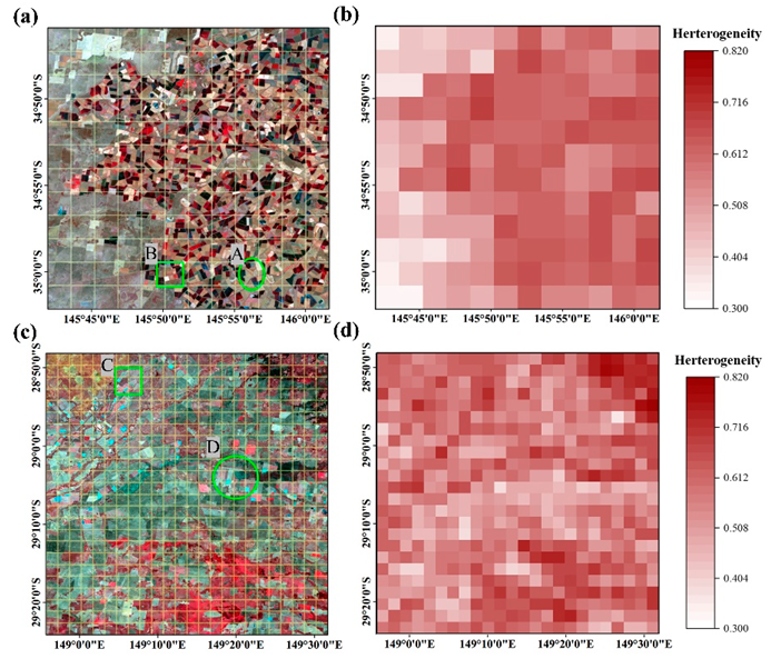
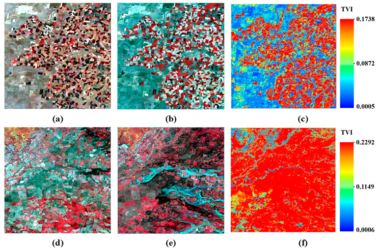
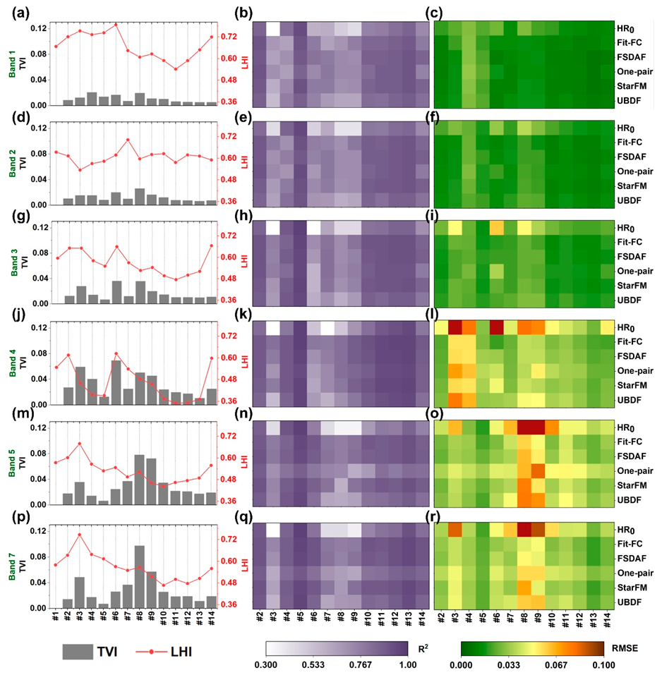
3.3. Spatial Heterogeneity and Temporal Variation Indices

The spatial heterogeneity and temporal variation of a landscape between t₁ and t₂ are the two main factors affecting STIF model performances [4]. In this study, we adopted the Landscape Heterogeneity Index (LHI) and Robust Change Vector Analysis (RCVA) algorithms to represent spatial heterogeneity and temporal variation, respectively, and examined their impacts on the performances of STIF methods.

LHI was proposed by Chen and Xu [40] with the aim of measuring landscape heterogeneity efficiently without any supporting data sets. It considers the individual patterns of both horizontal and vertical textures of landscapes. First, the differences between each pair of neighboring pixels along each row or column of the image are calculated; then the differences are classified as binary values (“1” denotes change and “0” denotes no change) using a direct difference threshold (DDT) or slope projection (SP) method. The LHI index is then calculated as:

$$LHI=(\frac{{\displaystyle {\sum }_{i=1}^L{\displaystyle {\sum }_{j=1}^{P-1}{r}_h(j,i)}}}{L(P-1)}+\frac{{\displaystyle {\sum }_{j=1}^P{\displaystyle {\sum }_{i=1}^{L-1}{r}_v(j,i)}}}{P(L-1)})/2,$$

(4)

where r_h (j,i) denotes the binary value depicting whether the surface reflectance of the jth pixel in the ith row is significantly different from the (j + 1)th pixel of the same row in the horizontal direction. Similarly, r_v (j,i) denotes the binary value in the vertical direction; L and P denote the total number of rows and columns, respectively. LHI represents the average rate of significant change among neighboring pixels in the horizontal or vertical direction in a given study region, and has been verified in experiments on urban extension analysis and seasonal change monitoring wetland area [40]. In this study, LHI was calculated based on each Landsat image on t₁ and the SP method was used to calculate LHI. Detailed descriptions of LHI calculation is referred to Chen and Xu [40]. Figure 2 demonstrates the patch-based LHI maps based on Coleambally (Figure 2a) and Gwydir (Figure 2c) Landsat images acquired on 4 December 2001 and 26 November 2004, respectively. The LHIs of all bands were averaged to obtain the heterogeneity grid map. The results shown in this grid map are consistent with our visual perception. The west part of the Coleambally area contains fewer land cover types than the east part. Correspondingly, LHI in the west (around 0.3–0.4) is lower than that in the east (over 0.6).

RCVA is a change detection technique proposed by Thonfeld et al. [46]. It is an improved version of the widely used Change Vector Analysis (CVA). The RCVA algorithm calculates change intensity and change direction, providing information on the spectral behavior of the change vector. From the change intensity, change or no-change discrimination is determined by defining a threshold. In this study, the magnitude of change was used as temporal variation index (TVI) and is calculated as:

$${\mathrm{TVI}}_i=\sqrt{{\sum }_{i=1}^{\mathrm{n}}{x_{diffi}}^2},$$

(5)

where ${\mathrm{TVI}}_i$ is the temporal variation index at band i, $x_{diffi}$ is the difference between Landsat surface reflectance at t₂ and t₁ of each band i, and n is the number of bands. $x_{diffi}$ is calculated as:

$$x_{diff{a}_i}(j,k)=\underset{(p\in \left[j-w,j+w\right],q\in \left[k-w,k+w\right])}{\min }(x_{2_i}(j,k)-x_{1_i}(p,q))\ge 0,$$

(6)

$$x_{diff{b}_i}(j,k)=\underset{(p\in \left[j-w,j+w\right],q\in \left[k-w,k+w\right])}{\min }(x_{1_i}(j,k)-x_{2_i}(p,q))\ge 0,$$

(7)

$$x_{diffi}=\{\begin{array}{c}{x}_{diff{a}_i},if{x}_{diff{a}_i}>0\\ 0-x_{diff{b}_i},if{x}_{diff{a}_i}=0\end{array},$$

(8)

where (j,k) is the position of the target pixel in a moving window with size (2w + 1) $\times$ (2w + 1). (p,q) are the adjacent pixels of the target pixel in the moving window. Figure 3 demonstrates the pixel-based TVI maps based on Coleambally (Figure 3c) and Gwydir (Figure 3f) Landsat images, respectively. The TVSs of all bands are averaged to obtain the temporal variation map. The results shown in this map are also consistent with our visual perception. The temporal variation of vegetation in the Southern Hemisphere from December to January is very intense, which is evident in Coleambally’s TVI map: the TVI values of vegetation areas are generally greater than 0.1, while less than 0.05 in non-vegetation areas. The temporal variation of most areas in Gwydir is very intense (greater than 0.1), while the variation of river is very small (less than 0.02). The characteristics shown in the figure are in good agreement with the actual variation of reflectance for river.

In this study, LHI and TVI were calculated at both scene scale and local scale. Local-scale LHI and TVI were derived by dividing Landsat images into small blocks with size of 100 × 100 pixels. The number of pixels with each block is large enough for calculating robust LHI and TVI, and the LHI and TVI calculated within each block allows us to examine the spatial distribution of landscape heterogeneity and temporal variation. Combined with model performances within the blocks, we examined the sensitivities of the STIF models in terms of LHI and TVI at local scale.

4. Results

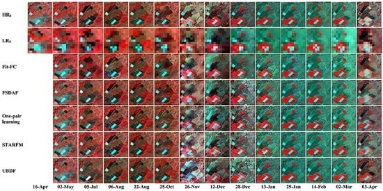
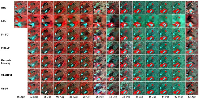
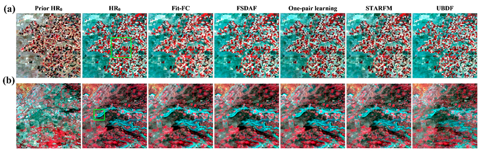
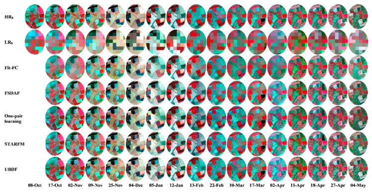
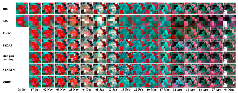
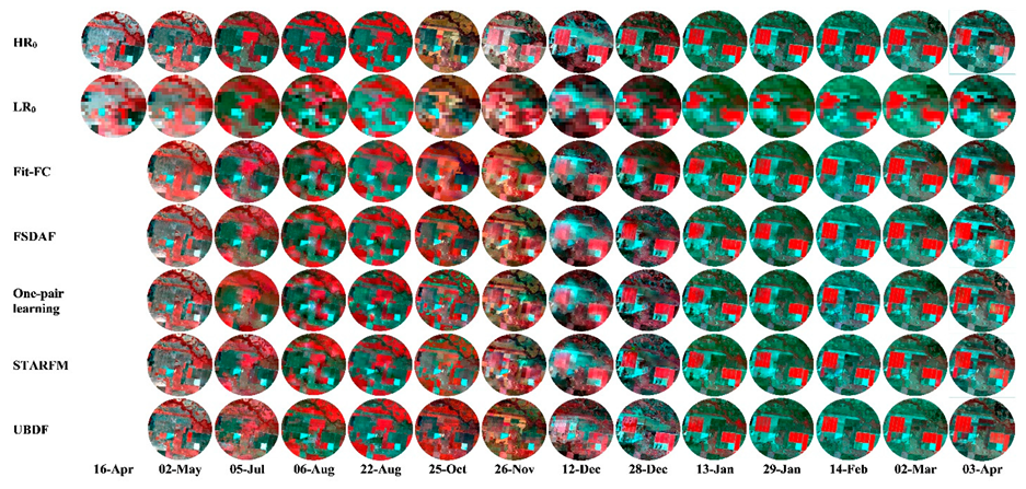
4.1. Visual Evaluations

In our experiment, the high-and low-resolution images of the previous moment and the low-resolution image of the latter moment are used as inputs, and the fusion result is compared with the high resolution image of the latter moment. Figure A1, Figure A2, Figure A3 and Figure A4 in Appendix A show the fusion results of the local regions on all prediction dates, focusing on the areas in the green circles in Figure 2a,c. At a glance, all models reasonably predicted the reflectance change, and the predicted images showed very high similarity with the actual image in terms of overall image hue. Figure 4 shows the predicted Landsat-like images as well as actual Landsat images (“HR₀” in Figure 4) over Coleambally on 5 January 2002 (Figure 4 top row; “HR₀” is image #7 in Table 1) and over Gwydir on 12 December 2004 (Figure 4 bottom row; “HR₀” is image #8 in Table 1). Their base pair MODIS-Landsat (see Figure 2) images were acquired on 4 December 2001 and 26 November 2004, respectively. These images were selected for visual examination as both study sites showed considerable temporal change from base date to prediction date. Coleambally showed intense phenology-induced surface reflectance changes due to vigorous growth of crops from December to January, while Gwydir showed large-area land cover type change from dryland to water. For visual evaluation, we used simulated MODIS images aggregated by Landsat images instead of real MODIS images in order to avoid radiometric and geometric inconsistencies between two sensors, and focusing solely on the performances of the methods [6,7,15]. Figure 4 shows that all models could generally capture the boundaries of heterogeneous crop fields and predict the color change of most fields in Coleambally site. In the Gwydir site where land cover types have substantially changed, it appears that all models face greater challenges, especially around the inundated areas. The boundaries of the inundated areas on the predicted images have a blurring effect when compared to the actual image, and the “rivers” appear wider than those in the actual image. In particular, the blurring effect in the Fit-FC-predicted image is more visible than that in the FSDAF- and one-pair learning-predicted images. The UBDF model failed to delineate the spatial details of the inundated areas.

The overall visual comparisons in Figure 4 did not show substantial differences among the five models, especially in the Coleambally site. Zoomed-in areas within the green boxes in Figure 4 are shown in Figure 5 and Figure 6 to examine the spatial details of the results. From the base date to prediction date in Coleambally site (Figure 5a,b), the hue of many small crop parcels changed from dark red to light red in the false color composite images, while the boundaries of the crop fields remained the same. Each of these parcels occupied one or two pixels in MODIS images, and each MODIS pixel contains two or more types of objects (Figure 5c,d). Generally, all predicted images had similar tone with the actual images on the prediction dates. However, the models showed different performances in some areas with intense temporal change. As shown in the two green rectangles in Figure 5, the color of the crop parcels changed from dark to red in false color composite image and the reflectance of the near-infrared band of the cropland varies greatly (approximately from 0.09 to 0.21). The tone of predicted images of the Fit-FC and the FSDAF are the closest to the actual image on the prediction date, while the results of one-pair learning, STARFM and UBDF models are closer to the prior image. The two yellow ellipses (Figure 5) show some small crop parcels with inconsistent change in color. Some parcels in the yellow ellipses changed from non-vegetation to vegetation, and the others experienced different vegetation growth periods. For these small parcels, Fit-FC, one-pair learning and STARFM show a “hazy” effect around the boundaries of the parcels, which has also been illustrated in previous research, for example, in Figure 7 and Figure 8 in Wang and Atkinson [6] and in Figure 8 in Zhao et al. [5]. It appears that the reflectance from one-pair learning in the small dryland parcel was affected by that of the surrounding crop parcels. The edges of crop parcels in the FSDAF- and UBDF-predicted images are better maintained, while the UBDF-predicted parcels have similar tones as those in the base image.

The zoomed-in area at the Gwydir site (Figure 6a,b) showed that many pixels experienced abrupt change from dry land to water. One-pair learning and FSDAF models yielded the best predictions for the inundated area; both models well represented the tone and the shape of the inundated area, although one-pair learning showed slightly hazy effect. Fit-FC produced slightly smaller inundated area, while STARFM predicted larger inundated area than the actual image. The result of UBDF over the inundated area was incorrect, which resulted in obvious “blocky effect” around the inundated area. Our visual impressions are similar as reported in Zhu et al. [7], which compared FSDAF, STARFM and UBDF over the same study site. Outside the inundated area, the regular-shaped crop fields in the green box in Figure 6 also demonstrated the differences in model predictions. Similar to the Coleambally site, Fit-FC and one-pair learning did not produce clear boundaries of the crop fields. On the other hand, FSDAF, STARFM and UBDF well delineated the crop field boundaries, while UBDF did not result in accurate prediction of the reflectance.

The green ellipse in the inundated area contains a river, about 1-2 Landsat pixel widths. The river was very blurry in the fusion results of Fit-FC, One-pair and STARFM, but FSDAF and UBDF can clearly see the river. The yellow ellipse area also contained a narrow river which became wider on the prediction date; surrounding a dryland area was also darker than that on the base date. It seems that Fit-FC could not obtain such small linear objects. The small linear objects obtained by one-pair learning were not very clear, either. FSDAF and UBDF clearly depict the linear objects, indicating the advantages of unmixing in predicting small objects [7]. However, it should be noted that none of these methods successfully predicted the change of the narrow river, indicating difficulties of all five STIF models in predicting change in small objects.

4.2. Scene-Level Accuracy Assessment

Figure 7 and Figure 8 show the TVI, LHI and model performances represented by R² and RMSE for bands 1 to 7 (blue, green, red, near infrared (NIR), shortwave infrared, SWIR1, and SWIR2) of the sequential-date Landsat data cubes for Coleambally and Gwydir sites, respectively. Please note that hereafter we used the real MODIS images for prediction. The TVI values at the Gwydir site are much higher than those at the Coleambally site, especially in bands 4, 5, and 7, which can be explained by abrupt reflectance change due to intense flood inundation. In Coleambally, substantially higher TVI values were found in image #7 (from 04 December 2001 to 05 January 2002) and #9 (from 12 January 2002 to 13 Febuary 2002) in bands 4 and 5 as a result of irrigation and crop growth. Figure 7 and Figure 8 also show the R² and RMSE between the target image and the prior image, denoted as HR₀ (top rows of accuracy matrices of Figure 7 and Figure 8). A higher RMSE of HR₀ indicates lower consistency between the prior and target images, i.e., a higher temporal variation. The time-series patterns of TVI (left column in Figure 7 and Figure 8) are very similar to those of the RMSE of HR₀ (right column in Figure 7 and Figure 8) for each band at both sites, indicating that TVI can reasonably represent the intensity of change. The spatial heterogeneity in Coleambally decreases (from image #1 to #8) and then increases gradually for all bands except band 4. Due to the different growing stage of crops, the NIR image became slightly more heterogeneous. Gwydir comprises heterogeneous pastures and riparian vegetation which were covered by natural flood during December. The heterogeneity of the Gwydir area has gradually decreased from October to January (from image #6 to #11) due to the transition from greening vegetation to water dominance during this period.

The accuracy matrices in the middle and right columns of Figure 7 and Figure 8 demonstrate that all models have much greater variability in performances in Gwydir site than that in Coleambally site. The R² values range from 0.48 to 0.98 in Colleambally site, and from 0.34 to 0.97 in Gwydir site; the RMSEs range from 0.004 to 0.067 in Colleambally site, and from 0.003 to 0.082 in Gwydir site. It is obvious that temporal variation between the prior and target dates greatly affected the performances of all models. For the Coleambally site, the most obvious examples are band 4 images #7 and #9 (Figure 7k,l). It is difficult to obtain accurate prediction results in this case (R² range from 0.54 to 0.68 and RMSEs range from 0.05 to 0.07) as a result of great change intensity (TVI > 0.04). TVI values of bands 1, 2 and 3 are lower than those of bands 4, 5, and 7; correspondingly, performances of all models for bands 1, 2, and 3 are better than those for bands 4, 5, and 7. For Gwydir site, the TVI values of band 4 of image #3 and #6, those of band 5 and band 7 of images #8 and #9 were greater than 0.06; correspondingly, R² of all models are lower than 0.79 and RMSE are higher than 0.04. When change intensity is strong, we found that Fit-FC and FSDAF both had similar accuracy and performed better than other models. This is consistent with Wang and Atkinson [6], which reported that Fit-FC performed slightly better than FSDAF in Coleambally site and much better than STARFM and UBDF models. In our study, we also found that one-pair learning and STARFM performed similar, and better than the UBDF model. Nonetheless, most of the RMSEs of the predicted images are much lower than those of HR₀, indicating the necessities of the STIF models.

However, we also found that in a few cases, the STIF-predicted images are not necessarily more accurate than HR₀. This situation often occurs for images with very small TVI values such as #8 in Coleambally (Figure 7) and #5 in Gwydir (Figure 8). STARFM, FSDAF and Fit-FC use the information of similar pixels in a neighborhood in the spatiotemporal fusion process. If the reflectance difference between the predicted time and the base time is large, the use of similar pixels can improve the accuracy of spatiotemporal fusion significantly. However, if the temporal variation between two images is very small, the use of similar pixels may introduce new errors.

Spatial heterogeneity is another factor affecting the performance of models, while different models have different sensitivities to spatial heterogeneity. Compared to other models, performances of Fit-FC seem to be more easily affected by greater spatial heterogeneity. For example, images #14–#17 (bands 1, 2 and 3) for Coleambally site, and images #3 and #6 (band 1) for Gwydir site have considerably higher LHI values than other dates, and Fit-FC produced evidently lower accuracies than the other models. Please note that those images have relatively low change intensities, where STIF models are expected to perform well. Different from STARFM which is another weight function-based model, Fit-FC uses a local regression model to capture spectral changes from t₁ to t₂. The local regression fitting inevitably brings about blocky artifacts [6]. Although spatial filtering and residual compensation were then applied to eliminate the blocky artifacts, these operations seem to have limited effects in regions with strong heterogeneity. There are also images on some dates having both high spatial heterogeneity and high temporal variations, such as band 4 of image #7 at the Coleambally site, bands 5 and 7 of image #3, bands 3 and 4 of image #6 in Gwydir region. For these situations, Fit-FC and FSDAF both produced better results than the other models. The heterogeneous region with a strong temporal change is very difficult to deal with for STIF models. It shows that the advantage of Fit-FC in dealing with strong temporal changes may compensate for its shortcomings in the region of strong heterogeneity.

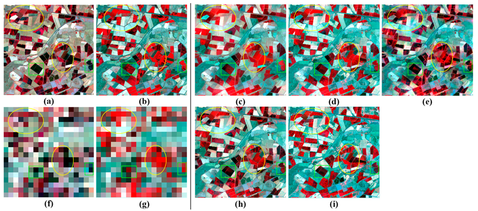
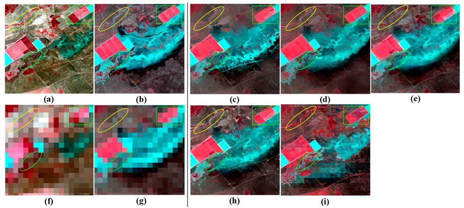
4.3. Local-Level Comparisons

STIF models have been frequently used to generate synthesis images over small regions of interest for applications such as field-scale crop yield estimation [47], evapotranspiration estimation [38,48], and flood inundation detection [33,49]. Thus, it is necessary to evaluate how local-scale spatial heterogeneity and temporal variation affect model performances [4]. To do this, each image was divided into image blocks with each block containing 100 × 100 pixels (Figure 2). For each block, TVI and LHI were calculated per band to represent local-scale temporal variation and spatial heterogeneity; ERGAS and SSIM values of STIF-predicted images were calculated as indicators of model performances. The blocks within each single-band image were further classified into three types: (1) blocks with LHI above 75 percentile and TVI above 75 percentile represent high spatial heterogeneity and high temporal variation, denoted as “HH”; (2) blocks with LHI above 75 percentile and TVI below 25 percentile represent high spatial heterogeneity and low temporal variation, denoted as “HL”; and (3) blocks with LHI below 25 percentile and TVI above 75 percentile represent low spatial heterogeneity and high temporal variation, denoted as “LH”. For Coleambally, HL or LH blocks did not exist for some images because phenological change mainly occurred at heterogeneous crop fields. Therefore, 70 and 30 percentiles were used define the threshold of high or low LHI (or TVI), respectively. For the blocks of each type on each image, the model with the lowest average ERGAS value or the highest average SSIM value was selected as the optimal model.

Figure 9 and Figure 10 demonstrate the occurrences of each model identified as the optimal one based on ERGAS (upper row) and SSIM (bottom row) for the six bands at each date. For example, for HH blocks in Coleambally site on date #4 (Figure 9a), Fit-FC and one-pair learning produced the lowest average ERGAS value at five bands and one band, respectively. Generally, Fit-FC and FSDAF were most frequently identified as the optimal ones in terms of the ERGAS value, which assesses the accuracies of reflectance prediction (Figure 9). For both Coleambally and Gwydir, Fit-FC showed obviously a lower best-model frequency for “HL” blocks (Figure 9b and Figure 10b) than for “HH” and “HL” blocks (Figure 9a,c, Figure 10a,c). This is consistent with the image-level evaluation in Figure 7 and Figure 8, which show that Fit-FC produced lower R² and higher RMSE at images with high spatial heterogeneity and low temporal variation (e.g., Image #14–17 band 1 in Coleambally site). For Coleambally where phenological change dominates the spectral change across the image, FSDAF possesses the highest frequencies of the best model in terms of ERGAS for blocks with high heterogeneity and low change intensity (Figure 9b).

Evaluation in terms of SSIM values produced somewhat different results (Figure 9d–f, Figure 10d–f). SSIM examines the consistency of image textures between predicted and actual images [7]. Although Fit-FC performed well in “HH” and “LH” blocks in terms of ERGAS values, the occurrences of Fit-FC as the optimal model greatly decreased when SSIM was evaluated, especially at Coleambally. In comparison, FSDAF were more stable. It is notable that one-pair learning stands out to be frequently selected as optimal ones for both sites, although it was the best one occasionally in terms of ERGAS value. Here we focus on the performances of each model on image #8 at Gwydir as it was the only time that recorded the information of flood. The inundated area experienced strong temporal change from #7 to #8; therefore, the results of “HH” and “LH” blocks are emphatically analyzed. One-pair learning performed best for “HH” and “LH” blocks at #8 in terms of SSIM, followed by FSDAF. This result was consistent with the visual evaluation in Section 4.1, which showed that both models well captured the tone and shape of the inundated area. STARFM performed well in “HL” blocks at Gwydir site in terms of SSIM values. For both sites, UBDF showed a lower best-model frequency than the other four models.

5. Discussion

5.1. Model Characteristics and Applicable Situations

In this study, a total of thirty-one Landsat-MODIS image pairs with various spatial heterogeneities and temporal change intensities were used for model evaluation. The five STIF models all performed similarly well for landscapes with low spatial heterogeneity and temporal variation, while they showed different sensitivities to increasing spatial and temporal variations. In our experiment, both scene-level and local-level analyses showed that FSDAF is a very robust method in terms of reflectance and image structure accuracy, although it is not always the best one with the lowest error. The key of the FSDAF model to obtain accurate spectral change in phenology change-dominated Coleambally is the unmixing process. Unlike the UBDF model, it uses global unmixing rather than sliding windows-based unmixing. Global unmixing filters coarse pixels, eliminating the coarse pixels that may experience land-cover type change. By using the “purest” coarse pixels for global unmixing, the changes for small objects are considered, and the “collinear problem” that may occur in the unmixing equation can also be solved. Moreover, FSDAF can achieve better results in the change of land cover type (Gwydir site) compared to STARFM, UBDF and Fit-FC, because it distributes the residuals based on the result of TPS to deal with the change of land cover types [39]. TPS prediction uses spatial dependence of the coarse pixels and captures the spatial patterns shown in the coarse image. By using TPS, residual distribution not only ensures that the re-aggregated fused fine-resolution image exactly matches the original coarse resolution image, but also help to improve accuracy of individual subpixels. Previous research also reported better accuracy of FSDAF compared to STARFM and UBDF in various application scenarios [7,50,51,52]. Please note that FSDAF has some shortcomings. For example, the assumption that errors in residual distribution depend mainly on landscape homogeneity has no theoretical basis [52]. Furthermore, in the last step of FSDAF, the fusion results are obtained by a weighted function using similar pixels which were searched from fine image at t₁. This operation is based on the premise that there is no land-cover type change. Once the land-cover type changed, the last step may lead to errors.

The Fit-FC model performed well for landscapes or regions with high TVI in terms of the predicted spectral reflectance accuracy. To date, few studies have applied Fit-FC model or compared with other models as it was proposed recently. Wang and Atkinson reported that Fit-FC was more accurate than FSDAF and STARFM in terms of correlation coefficient (CC), RMSE and universal image quality index over two sites with considerable phenological change [6], which was consistent with our study. In our study, we further found that Fit-FC is not suitable for landscapes/regions with low TVI and high LHI, and its performance in terms of retaining the image structure was not as good as FSDAF, one-pair learning, or even STARFM. From the principle of Fit-FC, it first uses a local linear regression model to find the relationship between coarse resolution images at t₁ and t₂, and applies this relationship to the fine resolution images. This in general could reduce the difference between the predicted image and the MODIS image at t₂. For scenarios of strong phenological change, the regression model can greatly reduce the difference between the predicted image and the MODIS image at t₂, as the interim coarse-fine image pair established by the regression model has much greater relation with the observations at t₂. However, in the local RM step all the fine pixels in a coarse pixel share the same set of coefficients for prediction. This strategy is reasonable in relatively homogeneous regions, which could explain that Fit-FC is frequently selected as the best one in “LH” blocks (Section 4.3). However, this may not be true in heterogeneous regions because land objects within a coarse pixel may not have the same temporal trend. In addition, the local RM introduces “blocky artifacts”. Although SF in the second step intended to alleviate the blocky effect, it also introduced blurring or hazy effect (see Figure 5b and Figure 6b in Wang and Atkinson [6]) because weighted average filters were applied across the image. Therefore, Fit-FC produced lower SSIM values for local analysis than the other models, and the spatial details of the object boundaries tended to be lost (see Figure 5c and Figure 6c).

The performance of one-pair learning in restoring spectral values is not as accurate as Fit-FC or FSDAF models (Figure 7, Figure 8, Figure 9 and Figure 10), while its ability for recovering the image structures was better than the Fit-FC model (Figure 9 and Figure 10). In addition, it is good at capturing large-scale land cover change, which was also reported in Chen et al. [30], Zhao et al. [5], and Song et al. [28]. The inundated area restored by one-pair learning is more similar as that on the observed image (Section 4.1). Different from STARFM, Fit-FC and UBDF, one-pair learning improves the change delineation accuracy in the prediction image by increasing the spatial resolution of MODIS data. This strategy can well restore the spatial distribution information of various objects at t₂. One-pair learning trains the dictionary pair on the Landsat and MODIS images at t₁ and then super-resolve the MODIS image at t₂ using a sparse coding technique. The dictionary pair captures the structure similarity between Landsat and MODIS images, which is then used to simulate the features at t₂. Even if there is land cover change from t₁ to t₂, the learning strategy can still predict image structure as long as all land cover types at t₂ can be found at t₁ [43]. The next important step is a high-pass modulation. In this step, the Landsat image at time t₁ and the downscaled MODIS image at t₁ reconstructed by the trained dictionaries are subtracted to obtain high-frequency information. This high-frequency information helps to enhance the spatial details in prediction, and thus obtains relatively accurate results in terms of SSIM. It should be noted that the sparse representation method has been widely used in natural image field in order to improve the image resolution two or three times. For the task of STIF, a MODIS image need to be downscaled 16–20 times to have the same resolution of Landsat. Although one-pair learning solves this problem using a two-layer framework where a MODIS image is downscaled 2–4 times to a transition image in the first layer, and then downscaled to 30 m in the second layer, the spectral information of different objects was recovered only through the dictionaries trained at t₁. It may cause errors in prediction of spectral values.

STARFM is probably the most widely used STIF model [4]. Its applications includes crop progress monitoring [47], evapotranspiration monitoring [38], flood mapping [33], forest disturbance mapping [53], land surface temperature generation [39], and producing NDVI maps [52], etc. It has been widely recognized in the remote sensing community. Our results demonstrated that STARFM generally performed well for Coleambally site with gradual spectral change, although the spectral accuracies are slightly lower than those of the Fit-FC and FSDAF models (Figure 7). The good performances of STARFM for predicting gradual spectral change have also been demonstrated in application research such as Gao et al. [1,47] and Onojeghuo et al. [54]. Even for most images of Gwydir site (except images #8 and #9 where land cover type changed) in our study, STARFM restored well image structure for blocks with high heterogeneity and low temporal variation. However, it produced much less accurate prediction for the abrupt land cover change with shape change, which was also reported in Zhu et al. [7] when compared to FSDAF and in Zhao et al. [5] when compared to one-pair learning. This is probably because that the model is established based on the assumption that similar pixels change with a similar trend. The assumption may not be true if abrupt change occurs.

UBDF is the least recommended model for predicting land cover change in this study, although its overall accuracies for the Coleambally site are acceptable. Our results are consistent with the results of Zhu et al. [7] and Wang and Atkinson [6], which showed that the precision of UBDF was slightly lower than that of STARFM in terms of CC and RMSE for cases of phenological changes, but much lower than STARFM for cases of land-cover type changes (see Table 4 in Zhu et al. [7]). The basic assumption of this unmixing-based model is that the land-cover type does not change. For UBDF, the land-cover type change has a great impact on the accuracy of fusion results in the whole sliding window, including the areas without land-cover type changes. The UBDF model first classifies the Landsat image, and then obtains the reflectance change value for each class through a linear unmixing process. All coarse pixels within the sliding window are unmixed at the same time by solving least square equations; land-cover type change inevitably brings errors to the prediction results within the entire sliding window. When compared to STARFM, the sliding window size of UBDF is much larger (7*7 MODIS pixels vs. 31*31 Landsat pixels in our experiments). Therefore, UBDF is more affected by land-cover type change compared to STARFM. One significant advantage of UBDF is, though, that if there is no land-cover type change, it can well retain the edge information of objects (green ellipse in Figure 6).

Another factor that may limit the wide application of STIF models lies in the computing efficiency. In our study, STARFM, UBDF and FSDAF were implemented in ENVI 5.3/IDL 8.5, and Fit-FC and one-pair learning models were implemented in MATLAB R2018b. All models ran on Windows 10 platform with Intel i7-8750H CPU and 16.0GB RAM. Because the models ran on different platforms, we re-implemented the UBDF model on the MATLAB platform. The UBDF models of the two platforms adopt the same parameters and were tested in the Coleambally area. The results showed that the time spent on the two platforms was 279 s (ENVI/IDL) and 267 s (MATLAB), respectively. The time difference is less than 5%. Therefore, the time-consuming of the two platforms are comparable. As listed in

Table 3. Comparison of model runtime (unit: seconds) of the five models for two study sites.

Study Site (Landsat Image Size)	Fit-FC	FSDAF	One-Pair Learning (Training/Prediction)	STARFM	UBDF
Coleambally (1200 × 1200)	149	473	952/81	207	279
Gwydir (2400 × 2400)	603	1864	2976/348	806	1054

, Fit-FC is the fastest among all models. It takes about 4 min for Coleambally site with an area of 1296 km², and 15 min for Gwydir site with an area of 5184 km². The RM step of the Fit-FC model takes less than one second at the Coleambally site. The model runtime is mainly in the weighted calculation of similar pixels. Compared to STARFM that also includes weighting similar pixels, Fit-FC takes much less time as it only selects 20 pixels with the most similar spectra, while STARFM needs to calculate the weights of all similar pixels that meet the requirements. FSDAF was less efficient than Fit-FC, STARFM and UBDF models. This is because FSDAF has more steps, including temporal prediction and spatial prediction, and the final step using information in neighborhood predicts the simulated fine image pixel by pixel, like the procedure of STARFM. One-pair learning model takes much time to train the dictionaries; but once the dictionaries are constructed, it takes much less time to get the final prediction. Considering the computation efficiency, the Fit-FC model may be recommended for large area applications. If there is abrupt land cover change with shape change, the FSDAF model may be considered prior to one-pair learning.

Table 4. Summary of pros and cons of the five models identified in this study.

Model	Pros	Cons
Fit-FC	High reflectance accuracy for HL, HH and LH landscapes and image patches Computation efficient	Less accurate for LH landscapes and image patches Less effective in capturing image structure
FSDAF	Robust with stable results Good reflectance accuracy for both phenological and land cover type change	Less computation efficient compared to Fit-FC, STARFM and UBDF
One-pair learning	Good for large-area land cover type change with shape change Good for capturing image structure	Computationally intensive
STARFM	Good reflectance accuracy for heterogeneous landscapes with phenological change More computational efficient than FSDAF, one-pair learning and UBDF	Not suitable for land cover type change, especially with object shape change
UBDF	Acceptable reflectance accuracy for heterogeneous landscapes with phenological change	Lowest accuracy among the five models

summarizes the pros and cons of each model found in this research.

5.2. Limitations and Future Directions

STIF models have been widely used in monitoring phenological change, but it is more challenging to predict land cover type changes, especially the changes in the shape or boundary of objects [5]. The flooding of Gwydir in this study is a typical shape change. FSDAF and one-pair learning have made relevant considerations for shape change, but this was not considered in STARFM, UBDF, and Fit-FC. Although one-pair learning and FSDAF can achieve relatively higher accuracy in the case of shape change, none of these models can accurately capture the boundaries of the shape change area. A possible solution is to further improve learning-based models. Recent studies [26,27,28] have applied CNNs for spatiotemporal fusion, and obtained better results in shape change monitoring. Many spatiotemporal fusion models based on deep learning use super-resolution reconstruction strategies. In the field of remote sensing image super-resolution reconstruction, some researchers have compared the deep learning-based super-resolution reconstruction method with the traditional super-resolution reconstruction method in detail. Their research results show that SRCNN model is not necessarily better than sparse representation-based model [55]. It is also necessary to compare the spatiotemporal fusion method based on deep learning and the traditional spatiotemporal fusion method systematically in future research. However, the high computational complexity may limit the applications of deep learning algorithms in reconstructing time series Landsat-like datasets over large areas. Recently developed transfer-learning techniques may be introduced in the future in order to simplify the training process. In addition, the computation efficiency may be improved by replacing pixel-wise calculation with feature-level calculation or using parallel computing [4].

Another limitation is that none of the tested models can ideally capture changes of small objects. For example, when only a few fine pixels are involved in the change, the change is invisible in the low-resolution image (see the river in the yellow elliptical region in Figure 6 and the result analysis in Section 4.1). To accurately capture changes of small objects, two image pairs including one prior to and the other posterior to the prediction time is suggested, auxiliary data can be to provide related information for the tiny change at the prediction time. However, it is necessary to balance the difficulty of accessing multiple Landsat images and the significance of capturing the changes.

In addition to the problems mentioned above, some of the following issues are worthy of attention and further exploration in future research. The spatial resolution difference of corresponding multispectral bands between Landsat image and MODIS image is about 16 times; however, the resolution differences of other image pairs may be greater than 16 times or less than 16 times. As more and more remote sensing images are involved, which models can achieve better results with different resolution differences? In addition, how much influence does the time interval between the t₁ and t₂ have on the various models, how accurate the fusion result of different models on different landcover types is, and whether some models are more suitable for some specific landcover types? These questions are very interesting and worthy of further discussion.

6. Conclusions

In this paper, Fit-FC, FSDAF, one-pair learning, STARFM and UBDF models are compared using 31 Landsat-MODIS image pairs over two study sites representing seasonal phenological change and abrupt land cover type change. LHI and TVI are designed to describe spatial heterogeneity and change intensity, respectively. The performance of the models is analyzed in terms of their sensitivities to variations of LHI and TVI at both scene and local scales. Our results show that both LHI and TVI have great impact on model performances, while models have different sensitivities to variations of LHI and TVI. The conclusions are as follows: (1) FSDAF is the most robust model at both scene and local scales for both sites; it can predict both spectral reflectance and image structure relatively accurately. However, FSDAF is less computationally efficient than the other models except one-pair learning. (2) Fit-FC has the highest computing efficiency. It is accurate in predicting reflectance, especially for the cases of strong temporal change, but it is less accurate in capturing image structures and textures compared to FSDAF and one-pair learning. It is also less accurate than the FSDAF model in regions with high heterogeneity but low change intensity. (3) One-pair learning has advantages in prediction of large-area land cover change, and it is capable of preserving image structures. It is the least computationally efficient model since the training process of dictionary learning increases the computation complexity. (4) the STARFM model is good at predicting phenological change while it is not suitable for land cover type change, especially for the “shape change”. Because the model can be publicly accessible and its higher efficiency than FSDAF, it may be still the most applicable one in the near future. (5) UBDF is not recommended for the case of strong temporal changes or abrupt changes.

The findings of this study could help users select appropriate models for their own applications. For example, if STIF models are used to construct time series images for continuous monitoring of vegetation change over large study area, Fit-FC may be used because of its high computing efficiency and its accuracy in predicting reflectance change. If STIF models are used to detect large-area land cover change such as flood inundation, forest logging or urban expansion, FSDAF and one-pair learning may be used because they were more accurate in predicting structures of the changing images. In any cases, image pair with observation date closest to the prediction date should be used to minimize the impact of temporal variation. Future research are recommended to focus on accurately retrieving abrupt land cover change, change in small objects as well as improving the computation efficiency.

References

1. Gao, F.; Hilker, T.; Zhu, X.; Anderson, M.; Masek, J.; Wang, P.; Yang, Y. Fusing Landsat and MODIS data for vegetation monitoring. IEEE Geosci. Remote Sens. Mag. 2015, 3, 47–60. [Google Scholar] [CrossRef]
2. Hilker, T.; Wulder, M.A.; Coops, N.C.; Linke, J.; McDermid, G.; Masek, J.G.; Gao, F.; White, J.C. A new data fusion model for high spatial-and temporal-resolution mapping of forest disturbance based on Landsat and MODIS. Remote Sens. Environ. 2009, 113, 1613–1627. [Google Scholar] [CrossRef]
3. Weng, Q.; Fu, P.; Gao, F. Generating daily land surface temperature at Landsat resolution by fusing Landsat and MODIS data. Remote Sens. Environ. 2014, 145, 55–67. [Google Scholar] [CrossRef]
4. Zhu, X.; Cai, F.; Tian, J.; Williams, T.K.-A. Spatiotemporal Fusion of Multisource Remote Sensing Data: Literature Survey, Taxonomy, Principles, Applications, and Future Directions. Remote Sens. 2018, 10, 527. [Google Scholar] [Green Version]
5. Zhao, Y.; Huang, B.; Song, H. A robust adaptive spatial and temporal image fusion model for complex land surface changes. Remote Sens. Environ. 2018, 208, 42–62. [Google Scholar] [CrossRef]
6. Wang, Q.; Atkinson, P.M. Spatio-temporal fusion for daily Sentinel-2 images. Remote Sens. Environ. 2018, 204, 31–42. [Google Scholar] [CrossRef] [Green Version]
7. Zhu, X.; Helmer, E.H.; Gao, F.; Liu, D.; Chen, J.; Lefsky, M.A. A flexible spatiotemporal method for fusing satellite images with different resolutions. Remote Sens. Environ. 2016, 172, 165–177. [Google Scholar] [CrossRef]
8. Song, H.; Huang, B. Spatiotemporal satellite image fusion through one-pair image learning. IEEE Trans. Geosci. Remote Sens. 2013, 51, 1883–1896. [Google Scholar] [CrossRef]
9. Zhu, X.; Chen, J.; Gao, F.; Chen, X.; Masek, J.G. An enhanced spatial and temporal adaptive reflectance fusion model for complex heterogeneous regions. Remote Sens. Environ. 2010, 114, 2610–2623. [Google Scholar] [CrossRef]
10. Liu, M.; Liu, X.; Wu, L.; Zou, X.; Jiang, T.; Zhao, B. A modified spatiotemporal fusion algorithm using phenological information for predicting reflectance of paddy rice in southern China. Remote Sens. 2018, 10, 772. [Google Scholar] [CrossRef]
11. Wu, P.; Shen, H.; Zhang, L.; Göttsche, F.-M. Integrated fusion of multi-scale polar-orbiting and geostationary satellite observations for the mapping of high spatial and temporal resolution land surface temperature. Remote Sens. Environ. 2015, 156, 169–181. [Google Scholar] [CrossRef]
12. Wang, P.; Gao, F.; Masek, J.G. Operational data fusion framework for building frequent Landsat-like imagery. IEEE Trans. Geosci. Remote Sens. 2014, 52, 7353–7365. [Google Scholar] [CrossRef]
13. Shen, H.; Wu, P.; Liu, Y.; Ai, T.; Wang, Y.; Liu, X. A spatial and temporal reflectance fusion model considering sensor observation differences. Int. J. Remote Sens. 2013, 34, 4367–4383. [Google Scholar] [CrossRef]
14. Roy, D.P.; Ju, J.; Lewis, P.; Schaaf, C.; Gao, F.; Hansen, M.; Lindquist, E. Multi-temporal MODIS–Landsat data fusion for relative radiometric normalization, gap filling, and prediction of Landsat data. Remote Sens. Environ. 2008, 112, 3112–3130. [Google Scholar] [CrossRef]
15. Gevaert, C.M.; García-Haro, F.J. A comparison of STARFM and an unmixing-based algorithm for Landsat and MODIS data fusion. Remote Sens. Environ. 2015, 156, 34–44. [Google Scholar] [CrossRef]
16. Amorós-López, J.; Gómez-Chova, L.; Alonso, L.; Guanter, L.; Zurita-Milla, R.; Moreno, J.; Camps-Valls, G. Multitemporal fusion of Landsat/TM and ENVISAT/MERIS for crop monitoring. Int. J. Appl. Earth Obs. Geoinf. 2013, 23, 132–141. [Google Scholar] [CrossRef]
17. Zurita-Milla, R.; Kaiser, G.; Clevers, J.; Schneider, W.; Schaepman, M. Downscaling time series of MERIS full resolution data to monitor vegetation seasonal dynamics. Remote Sens. Environ. 2009, 113, 1874–1885. [Google Scholar] [CrossRef]
18. Zurita-Milla, R.; Clevers, J.G.; Schaepman, M.E. Unmixing-based Landsat TM and MERIS FR data fusion. IEEE Geosci. Remote Sens. Lett. 2008, 5, 453–457. [Google Scholar] [CrossRef]
19. Zhukov, B.; Oertel, D.; Lanzl, F.; Reinhackel, G. Unmixing-based multisensor multiresolution image fusion. IEEE Trans. Geosci. Remote Sens. 1999, 37, 1212–1226. [Google Scholar] [CrossRef]
20. Huang, B.; Zhang, H. Spatio-temporal reflectance fusion via unmixing: Accounting for both phenological and land-cover changes. Int. J. Remote Sens. 2014, 35, 6213–6233. [Google Scholar] [CrossRef]
21. Zhang, W.; Li, A.; Jin, H.; Bian, J.; Zhang, Z.; Lei, G.; Qin, Z.; Huang, C. An enhanced spatial and temporal data fusion model for fusing Landsat and MODIS surface reflectance to generate high temporal Landsat-like data. Remote Sens. 2013, 5, 5346–5368. [Google Scholar] [CrossRef]
22. Wu, M.; Niu, Z.; Wang, C.; Wu, C.; Wang, L. Use of MODIS and Landsat time series data to generate high-resolution temporal synthetic Landsat data using a spatial and temporal reflectance fusion model. J. Appl. Remote Sens. 2012, 6, 063507. [Google Scholar]
23. Huang, B.; Song, H. Spatiotemporal reflectance fusion via sparse representation. IEEE Trans. Geosci. Remote Sens. 2012, 50, 3707–3716. [Google Scholar] [CrossRef]
24. Moosavi, V.; Talebi, A.; Mokhtari, M.H.; Shamsi, S.R.F.; Niazi, Y. A wavelet-artificial intelligence fusion approach (WAIFA) for blending Landsat and MODIS surface temperature. Remote Sens. Environ. 2015, 169, 243–254. [Google Scholar] [CrossRef]
25. Liu, X.; Deng, C.; Wang, S.; Huang, G.-B.; Zhao, B.; Lauren, P. Fast and accurate spatiotemporal fusion based upon extreme learning machine. IEEE Geosci. Remote Sens. Lett. 2016, 13, 2039–2043. [Google Scholar] [CrossRef]
26. Liu, X.; Deng, C.; Chanussot, J.; Hong, D.; Zhao, B. StfNet: A Two-Stream Convolutional Neural Network for Spatiotemporal Image Fusion. IEEE Trans. Geosci. Remote Sens. 2019. [Google Scholar] [CrossRef]
27. Tan, Z.; Yue, P.; Di, L.; Tang, J.J.R.S. Deriving high spatiotemporal remote sensing images using deep convolutional network. Remote Sens. 2018, 10, 1066. [Google Scholar] [CrossRef]
28. Song, H.; Liu, Q.; Wang, G.; Hang, R.; Huang, B. Spatiotemporal Satellite Image Fusion Using Deep Convolutional Neural Networks. IEEE J. Sel. Top. Appl. Earth Obs. Remote Sens. 2018, 11, 821–829. [Google Scholar] [CrossRef]
29. Xu, Y.; Huang, B.; Xu, Y.; Cao, K.; Guo, C.; Meng, D. Spatial and temporal image fusion via regularized spatial unmixing. IEEE Geosci. Remote Sens. Lett. 2015, 12, 1362–1366. [Google Scholar]
30. Chen, B.; Huang, B.; Xu, B. A hierarchical spatiotemporal adaptive fusion model using one image pair. Int. J. Digit. Earth 2017, 10, 639–655. [Google Scholar] [CrossRef]
31. Emelyanova, I.V.; McVicar, T.R.; Van Niel, T.G.; Li, L.T.; van Dijk, A.I. Assessing the accuracy of blending Landsat–MODIS surface reflectances in two landscapes with contrasting spatial and temporal dynamics: A framework for algorithm selection. Remote Sens. Environ. 2013, 133, 193–209. [Google Scholar] [CrossRef]
32. Chen, B.; Huang, B.; Xu, B. Comparison of spatiotemporal fusion models: A review. Remote Sens. 2015, 7, 1798–1835. [Google Scholar] [CrossRef]
33. Zhang, F.; Zhu, X.; Liu, D. Blending MODIS and Landsat images for urban flood mapping. Int. J. Remote Sens. 2014, 35, 3237–3253. [Google Scholar] [CrossRef]
34. Li, A.; Bo, Y.; Zhu, Y.; Guo, P.; Bi, J.; He, Y. Blending multi-resolution satellite sea surface temperature (SST) products using Bayesian maximum entropy method. Remote Sens. Environ. 2013, 135, 52–63. [Google Scholar] [CrossRef]
35. Huang, B.; Zhang, H.; Song, H.; Wang, J.; Song, C. Unified fusion of remote-sensing imagery: Generating simultaneously high-resolution synthetic spatial–temporal–spectral earth observations. Remote Sens. Lett. 2013, 4, 561–569. [Google Scholar] [CrossRef]
36. Liao, L.; Song, J.; Wang, J.; Xiao, Z.; Wang, J. Bayesian method for building frequent Landsat-like NDVI datasets by integrating MODIS and Landsat NDVI. Remote Sens. 2016, 8, 452. [Google Scholar] [CrossRef]
37. Xue, J.; Leung, Y.; Fung, T. A Bayesian Data Fusion Approach to Spatio-Temporal Fusion of Remotely Sensed Images. Remote Sens. 2017, 9, 1310. [Google Scholar] [CrossRef]
38. Ke, Y.; Im, J.; Park, S.; Gong, H. Spatiotemporal downscaling approaches for monitoring 8-day 30 m actual evapotranspiration. ISPRS J. Photogramm. Remote Sens. 2017, 126, 79–93. [Google Scholar] [CrossRef]
39. Quan, J.; Zhan, W.; Ma, T.; Du, Y.; Guo, Z.; Qin, B. An integrated model for generating hourly Landsat-like land surface temperatures over heterogeneous landscapes. Remote Sens. Environ. 2018, 206, 403–423. [Google Scholar] [CrossRef]
40. Chen, B.; Xu, B. A novel method for measuring landscape heterogeneity changes. Remote Sens. Lett. 2015, 12, 567–571. [Google Scholar] [CrossRef]
41. Cheng, Q.; Liu, H.; Shen, H.; Wu, P.; Zhang, L. A spatial and temporal nonlocal filter-based data fusion method. IEEE Trans. Geosci. Remote Sens. 2017, 55, 4476–4488. [Google Scholar] [CrossRef]
42. Gao, F.; Masek, J.; Schwaller, M.; Hall, F. On the blending of the Landsat and MODIS surface reflectance: Predicting daily Landsat surface reflectance. IEEE Trans. Geosci. Remote Sens. 2006, 44, 2207–2218. [Google Scholar]
43. Yang, J.; Wright, J.; Huang, T.S.; Ma, Y. Image super-resolution via sparse representation. IEEE Trans. Image Process. 2010, 19, 2861–2873. [Google Scholar] [CrossRef] [PubMed]
44. Khan, M.M.; Alparone, L.; Chanussot, J. Pansharpening quality assessment using the modulation transfer functions of instruments. IEEE Trans. Geosci. Remote Sens. 2009, 47, 3880–3891. [Google Scholar] [CrossRef]
45. Wang, Z.; Bovik, A.C.; Sheikh, H.R.; Simoncelli, E.P. Image quality assessment: From error visibility to structural similarity. IEEE Trans. Image Process. 2004, 13, 600–612. [Google Scholar] [CrossRef] [PubMed]
46. Thonfeld, F.; Feilhauer, H.; Braun, M.; Menz, G. Robust Change Vector Analysis (RCVA) for multi-sensor very high resolution optical satellite data. Int. J. Appl. Earth Obs. Geoinf. 2016, 50, 131–140. [Google Scholar] [CrossRef]
47. Gao, F.; Anderson, M.C.; Zhang, X.; Yang, Z.; Alfieri, J.G.; Kustas, W.P.; Mueller, R.; Johnson, D.M.; Prueger, J.H. Toward mapping crop progress at field scales through fusion of Landsat and MODIS imagery. Remote Sens. Environ. 2017, 188, 9–25. [Google Scholar] [CrossRef] [Green Version]
48. Ke, Y.; Im, J.; Park, S.; Gong, H. Downscaling of MODIS One kilometer evapotranspiration using Landsat-8 data and machine learning approaches. Remote Sens. 2016, 8, 215. [Google Scholar] [CrossRef]
49. Dao, P.D.; Mong, N.T.; Chan, H.-P.J.G.; Sensing, R. Landsat-MODIS Image Fusion and Object-based Image Analysis for Observing Flood Inundation in a Heterogeneous Vegetated Scene. Gisci. Remote Sens. 2019. [Google Scholar] [CrossRef]
50. Chen, B.; Chen, L.; Huang, B.; Michishita, R.; Xu, B. Dynamic monitoring of the Poyang Lake wetland by integrating Landsat and MODIS observations. ISPRS J. Photogramm. Remote Sens. 2018, 139, 75–87. [Google Scholar] [CrossRef]
51. Latifi, H.; Dahms, T.; Beudert, B.; Heurich, M.; Kübert, C.; Dech, S. Synthetic RapidEye data used for the detection of area-based spruce tree mortality induced by bark beetles. Gisci. Remote Sens. 2018, 55, 839–859. [Google Scholar] [CrossRef]
52. Liu, M.; Yang, W.; Zhu, X.; Chen, J.; Chen, X.; Yang, L.; Helmer, E. An Improved Flexible Spatiotemporal DAta Fusion (IFSDAF) method for producing high spatiotemporal resolution normalized difference vegetation index time series. Remote Sens. Environ. 2019, 227, 74–89. [Google Scholar] [CrossRef]
53. Hilker, T.; Wulder, M.A.; Coops, N.C.; Seitz, N.; White, J.C.; Gao, F.; Masek, J.G.; Stenhouse, G. Generation of dense time series synthetic Landsat data through data blending with MODIS using a spatial and temporal adaptive reflectance fusion model. Remote Sens. Environ. 2009, 113, 1988–1999. [Google Scholar] [CrossRef]
54. Onojeghuo, A.O.; Blackburn, G.A.; Wang, Q.; Atkinson, P.M.; Kindred, D.; Miao, Y. Rice crop phenology mapping at high spatial and temporal resolution using downscaled MODIS time-series. Gisci. Remote Sens. 2018, 55, 659–677. [Google Scholar] [CrossRef] [Green Version]
55. Fernandez-Beltran, R.; Latorre-Carmona, P.; Pla, F. Single-frame super-resolution in remote sensing: A practical overview. Int. J. Remote Sens. 2017, 38, 314–354. [Google Scholar] [CrossRef]
Figure 1. Location of the Coleambally Irrigation Area and the Lower Gwydir Catchment.
Remotesensing 11 02612 g001
Figure 2. Examples of LHI maps. (a) Landsat color-infrared image (1200 × 1200 pixels) at Coleambally site acquired on 4 December 2001 divided into 12 × 12 blocks with each block containing 100 × 100 pixels; (b) the corresponding map of landscape heterogeneity index (LHI) calculated for each block. (c) Landsat color-infrared image (2400 × 2400 pixels) at Gwydir site acquired on 26 November 2004 divided into 24 × 24 blocks with each block containing 100 × 100 pixels; (d) the corresponding map of LHI calculated for each block. The time series prediction image of the sub region A, B, C and D in (a,b) will be presented in detail in Appendix A.
Remotesensing 11 02612 g002
Figure 3. Examples of TVI maps. (a,b) are the Landsat color-infrared images at Coleambally site acquired on 4 December 2001 and 5 January 2002; (c) is the corresponding map of temporal variation index (TVI) calculated for each pixel at Coleambally. (d,e) are the Landsat color-infrared image at Gwydir site acquired on 26 November 2004 and 12 December 2004; (f) is the corresponding map of LHI calculated for each pixel at Gwydir.
Remotesensing 11 02612 g003
Figure 4. Landsat images observed on prior date (Prior HR0) and prediction date (HR0), and the predicted Landsat-like images at (a) the Coleambally site and (b) the Gwydir site. Prior HR0 in Coleambally site was acquired on 4 December 2001, and HR0 was acquired on 5 January 2002; prior HR0 Gwydir site was acquired on 26 November 2004, and HR0 was acquired on 12 December 2004.
Remotesensing 11 02612 g004
Figure 5. Zoomed-in area (green rectangle area in HR0 of Figure 3a) of Landsat and MODIS image pairs at base date t1 (a,f) and prediction date t2 (b,g), as well as the simulated Landsat-like images predicted by Fit-FC (c), FSDAF (d), one-pair learning (e), STARFM (h) and UBDF (i).
Remotesensing 11 02612 g005
Figure 6. Zoomed-in area (green rectangle area in HR0 of Figure 3b) of Landsat and MODIS image pairs at base date t1 (a,f) and prediction date t2 (b,g), as well as the simulated Landsat-like images predicted by Fit-FC (c), FSDAF (d), one-pair learning (e), STARFM (h) and UBDF (i).
Remotesensing 11 02612 g006
Figure 7. Time series plot of TVI and LHI (a,d,g,j,m,p) and metrics of R2 (b,e,h,k,n,q) and RMSE (c,f,i,l,o,r) of each method for band 1, 2, 3, 4, 5, 7 (from top row to bottom row) for the whole Coleambally site. “HR0” denotes R2 and RMSE between target image and the prior image. The abscissa of all statistical charts is the image number in chronological order.
Remotesensing 11 02612 g007
Figure 8. Time series plot of TVI and LHI (a,d,g,j,m,p) and metrics of R2 (b,e,h,k,n,q) and RMSE (c,f,i,l,o,r) of each method for band 1, 2, 3, 4, 5, 7 (from top row to bottom row) for the whole Gwydir site. “HR0” denotes R2 and RMSE between target image and the prior image. The abscissa of all statistical charts is the image number in chronological order.
Remotesensing 11 02612 g008
Figure 9. Occurrences of optimal STIF models for “HH” blocks (a,d), “HL” blocks (b,e) and “LH” blocks (c,f) evaluated using ERGAS (top row) and SSIM (bottom row) at the Coleambally site.
Remotesensing 11 02612 g009
Figure 10. Occurrences of optimal STIF models for “HH” blocks (a,d), “HL” blocks (b,e) and “LH” blocks (c,f) evaluated using ERGAS (top row) and SSIM (bottom row) at the Gwydir site.
Remotesensing 11 02612 g010