Flood Mapping with Convolutional Neural Networks Using Spatio-Contextual Pixel Information


1
School of Electrical Engineering and Computer Sciences, Queensland University of Technology, Brisbane QLD 4000, Australia
2
Institute for Future Environments, Queensland University of Technology, Brisbane QLD 4000, Australia
*
Author to whom correspondence should be addressed.
Remote Sens. 2019, 11(19), 2331; https://doi.org/10.3390/rs11192331
Submission received: 12 July 2019
/
Revised: 30 September 2019
/
Accepted: 4 October 2019
/
Published: 8 October 2019
(This article belongs to the Special Issue Remote Sensing of Inland Waters and Their Catchments)
Abstract
:Remote sensing technology in recent years has been regarded the most important source to provide substantial information for delineating the flooding extent to the disaster management authority. There have been numerous studies proposing mathematical or statistical classification models for flood mapping. However, conventional pixel-wise classifications methods rely on the exact match of the spectral signature to label the target pixel. In this study, we propose a fully convolutional neural networks (F-CNNs) classification model to map the flooding extent from Landsat satellite images. We utilised the spatial information from the neighbouring area of target pixel in classification. A total of 64 different models were generated and trained with a variable neighbourhood size of training samples and number of learnable filters. The training results revealed that the model trained with neighbourhood sized training samples and with 32 convolutional filters achieved the best performance out of the experiments. A new set of different Landsat images covering flooded areas across Australia were used to evaluate the classification performance of the model. A comparison of our proposed classification model to the conventional support vector machines (SVM) classification model shows that the F-CNNs model was able to detect flooded areas more efficiently than the SVM classification model. For example, the F-CNNs model achieved a maximum precision rate (true positives) of 76.7% compared to 45.27% for SVM classification.
1. Introduction
Every year, flood incidents are accountable for huge impacts on social well being and economic infrastructure all over the world. Mapping flooding extent during a flood event has become a key tool needed to assist various private and government disaster management departments (local and state government emergency departments, and environmental groups) in mitigating, responding to and recovering from flood disasters [1,2,3]. Although these organizations seek different types of quantitative and qualitative information, their primary requirement is rapid acquisition of maps showing the extent of flood affected areas to plan relief work efficiently.
Traditionally, localised flood mapping was based on man-made ground surveys that requires skilled people to analyse [4]. However, with advancements in airborne technology, it is possible to conduct an aerial survey of extensive flooded areas for ground truth collection as we have observed in the studies by Damian Ortega-Terol et al. [5] where the authors proposed a low-cost aircraft-based survey that can help in classification for detection of large woody debris along a segment of Jucar River in Spain. In [3], the authors proposed a low-cost aerial photogrammetry method by combining a reduced cost passive sensors on board an ultra-light aerial platform to obtain precise topographic data from digital aerial images for flood hazard assessment in the upper basin of Adaja River in Spain. The aerial observation is, however, difficult for a flood event over a large geographical area since it requires enough time and resources [4,6]. Moreover, the adverse weather conditions could also be a hindrance for the aerial survey. With the advancement in on-board space-borne sensors, it has been possible to acquire flood data over large geographical areas from satellite images [2].
However, satellite imagery poses difficulties when it comes to information extraction, in particular, from multispectral images covering flooded areas because of the mixture of land and flood water components. The mixture of spectral properties of flood water and other land components in pixels makes visual classification difficult [7]. Most of flood mapping methods follow either of two approaches. The first approach is developing hydraulic or hydrologic models for mapping flooded areas, and the second approach is applying classification algorithms for mapping flooded areas. Flood inundation modelling is a complex hydrodynamic process that may contain large uncertainties [3,8]; for this reason, many researchers in their studies have proposed methods to improve over the flooding inundation modelling, as for example, in [3], where the authors proposed an integrated methods of geomatics and fluvial hydraulics to improve the information about flood behaviour.
Processes of accessing required ancillary data for hydraulic or hydrologic modelling is time consuming and can cause difficulty to obtain the rapid information during a flooding event. Numerous studies in recent years have proposed automated or semi-automated classification methods of flood mapping. These classification algorithms are based on statistical learning algorithms either assigning a label to each pixel (flood or non-flood) or determining the fractional coverage of each components present in a pixel [9]. Pixel-wise classification methods apply either rule-based thresholding methods or supervised machine learning models [10]. Rule-based classification methods usually generate image-specific threshold values to distinguish the water pixels from non-water pixels. Approaches like two-band water indices [11,12], and multi-band indices [13,14,15] are commonly adopted as rule-based methods using band algebra. In addition, statistical methods like principle component transform (PCT) [16] and independent component analysis (ICA) [17] have been applied for detecting the changes in information components between pre and post flood images of a region to identify flooded areas. The efficiency of the aforesaid methods depends on the identification of an optimum threshold which depends on a number of environmental factors like spatial resolution of the satellite image, presence of shadow and mixed pixels as stated by Pierdicca et al. [18]. Moreover, the optimal threshold values are required to be calibrated when mapped area on the ground changes [10] Therefore, it limits the generalisation ability of the rule-based methods for flood mapping.
Recently, with the availability of high spatial and spectral data, images are able to contain more complex details of land features; therefore, more sophisticated machine learning methods may be required to extract flooded information from those images. The most commonly adopted approach in this category is support vector machines (SVM) [19]. Artificial neural networks (ANN) is also considered a popular technique for mapping the spatial extent of floods due to their ability of handling multiple input data sources in the classification process as Kia et al. [20] have demonstrated. Studies like [7,21] applied decision tree classifiers for enhanced flood extent mapping. These classification methods provide high accuracy levels for localised flooding events, however, they lack generalisation ability and, hence, are not suitable for using multiple image applications. The performance of pixel-wise supervised classification models depends on sufficient and representative training samples especially while studying floods in a complex landscape. Compared to SVMs and decision tree classifier, ANN methods are more popular due to its easy adaptability and generalisation nature, but the model training is time consuming.
Furthermore, the interspersion of flood water with different ground cover types is often associated with high spectral variations of flood water pixels, which is difficult to take into account by pixel-wise classification methods. In the remote sensing literature, pixels that represent a mixture of spectral properties of different class types are termed as mixed pixels [22]. Spectral unmixing models like indices-based spectral unmixing [23], multiple end-member spectral mixture analysis (MESMA) [7], linear spectral unmixing [24] and Gaussian mixture model [25] are adopted for estimating the proportion of partial inundation from mixed pixels. Previously, we investigated linear spectral unmixing on extended support vector machines (u-eSVM) [26,27] to extract proportions of flood water from both pure pixels (pixels containing flood water) and mixed pixels. Later in [28], we proposed a Bayesian approach to enhance the previous classification results using u-eSVM by representing the probability values of flooding of each pixel instead of representing the flood fractional coverage of each pixel in the flood classification map.
In remote sensing, the object-based approach has also been proposed to deal with the problem of the complex spectral nature of flood waters in image processing [29,30]. Object-based classifiers utilize image spectral and spatial properties such as mean texture, shape and scale of an object to perform the classification. However, the use of these properties by themselves is not enough for flood extent mapping. The reason is because flood water is usually spread onto the other land cover types, creating inter-class spectral similarity alongside the intra-class spectral heterogeneity. Moreover, in a satellite image, a considerable amount of the recorded signal of each pixel originates from the surrounding area represented by that pixel [31]. In this context, the spectral information from neighbourhood pixels may offer great benefits over classic pixel-wise methods to distinguish pixels with similar spectral nature and assign them into appropriate classes [32].
Contextual classification is common in pattern recognition and computer vision. In remote sensing, using contextual spectral information offers an opportunity for studying flooding extent using neighbouring information. Recent developments in deep neural networks have shown the capability of convolutional neural networks (CNNs) to automatically learn image features utilising contextual information by a stack of learnable convolutional filters [33]. A recent work has applied convolutional neural networks for flood mapping by learning the change detection from a set of pre and post disaster aerial images [34]. The study demonstrated efficient classification using CNN methods, but it was limited to a single type of image with RGB channels for training the model. Nogueira et al. [35] in their study proposed four deep network architecture based on dilated convolutions and deconvolutions layers to distinguish between flooded and non-flooded areas from high resolution remote sensing images. The study outperforms all baseline methods by 1% in terms of Jaccard Index for flooding detection in a new location (unseen by the model network during training). The proposed method did not attempt to distinguish flood water and permanent water surfaces. Gebrehiwot et al. [36] used the pre-trained a VGG-based fully convolutional neural network model for flood extent mapping using unmanned aerial vehicles images. The classification results showed the model could get a precise level of classification accuracy with more than 90% accuracy value compared to 89% accuracy value of SVM classification but the study was limited to using RGB images.
In spite of the recent studies on convolutional neural network methods for detecting flooded areas, studies investigating the context-based fully convolutional neural networks (F-CNNs) on multispectral satellite images utilising six-image bands are not well documented in the literature as per our knowledge. Furthermore, no studies have attempted to apply convolutional neural networks to distinguish flood water from permanent water bodies using satellite images. Considering those facts, our proposed work makes use of contextual pixel information for semantic segmentation or pixel-wise detection of flooded areas. The idea of using training sample patches is adopted for utilizing the neighbouring-spectral properties to distinguish three class labels, namely: flood water class, permanent water class and non-water class. Areas are defined as flood-water class if they are normally dry but show presence of water during a flood event. Areas with frequent observation of water bodies are considered as permanent-water. Generally, water holes, river channels (containing seasonal or all season water), lakes and ponds are considered as permanent-water. Areas that remain always dry are labelled as non-water. Considering the limitation of the multispectral sensors of not being able to penetrate the vegetation cover to detect areas underneath, our proposed model does not address this scenario in the current approach.
In summary, the main objectives of this study are to: (1) develop a fully convolutional neural network model architecture that automatically detects flooded areas from multispectral remote sensing images; (2) to provide an empirical study that reveals the best architecture choice along with the best choice of neighbourhood size that produces consistent results of detecting flooded areas; (3) utilise the contextual spectral information of pixels to solve the problem of low accuracy of pixel-wise classification methods by not considering the pixels relation with its neighbouring pixel’s spectra for flood mapping.
2. Methodology and Data Processing
Our proposed classification methodology involves three distinct stages: Image pre-processing, training-validation and classification. Figure 1 represents the flowchart of the methodology we applied in this work.
2.1. Stage 1: Image Pre-Processing
The first stage involves registration of Landsat train images with corresponding reference images, preparation of initial dataset and from the initial dataset, selection of samples to develop train, validation and test set.
2.1.1. Landsat Data Collection
To train our proposed model we required a large dastaset which covers spectral properties of the three target class types. To the best of our knowledge, there is no publicly available large training databases of the flood water, permanent water and non-water class types for Australia. We have, therefore, tried to incorporate remote sensing images from various sources that helps to generate a training dastaset.
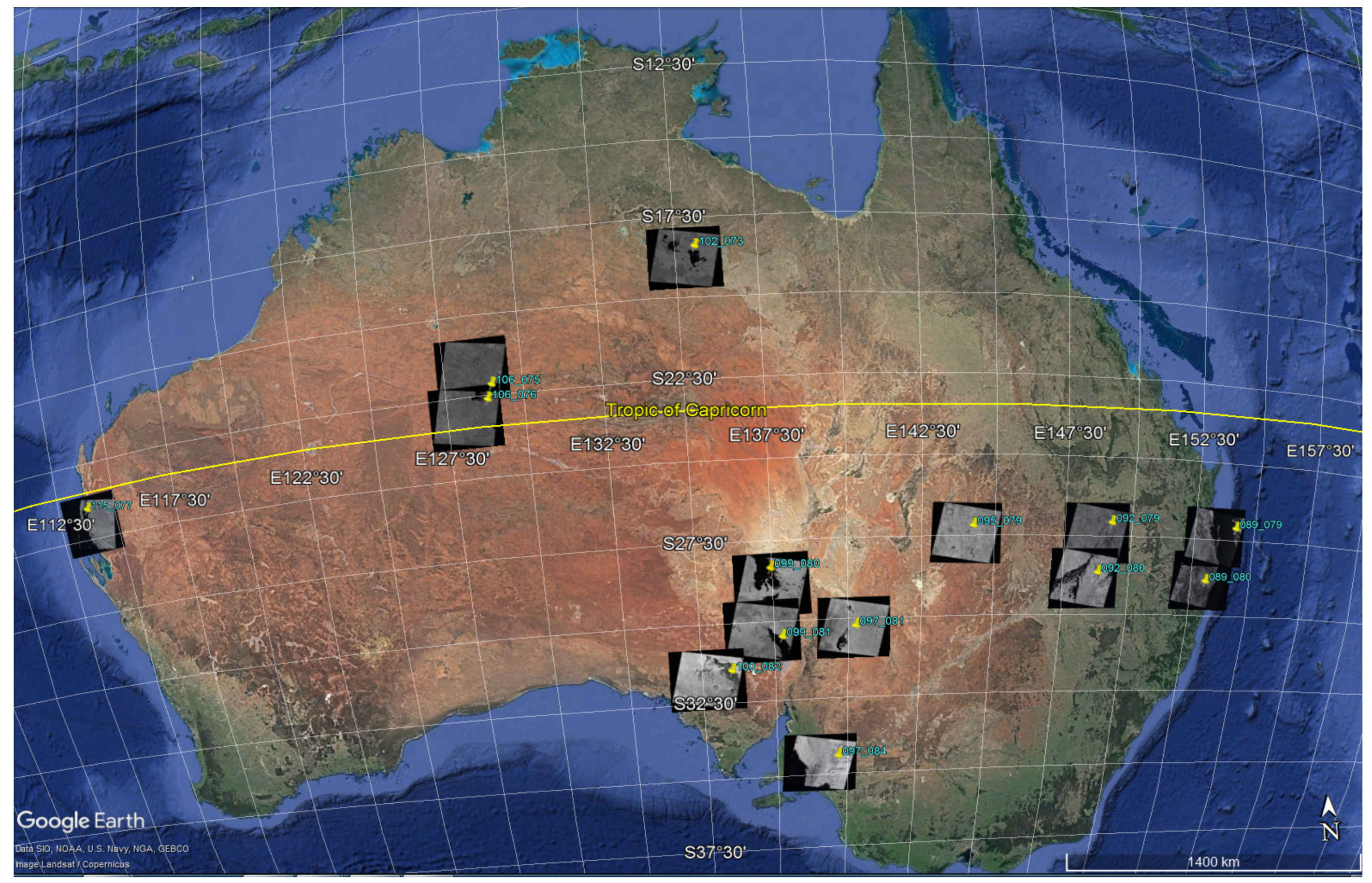
Recently, large remote sensing dastasets with low to medium spatial resolutions have been made available by scientific organizations around the world. Among them, Landsat images have most frequently been used for flood-related research due to their continuous observation of large areas with identical scene coverage. For example authors in studies- [11,12,13,14,16,17,19] used multispectral images obtained from Landsat sensors for mapping inundated areas. We have used Landsat-5 Thematic Mapper data that covers 2011 Queensland and New South Wales floods for our experiments. These images are distributed by the United States Geological Survey. Labels acquired from corresponding reference dastaset are utilized to generate training samples for each class. The dastaset is a collection of 14 images representing flooded areas captured during 2011 Queensland and NSW flood events and permanent water bodies from different parts of Australia of similar time period. The events of 2011 Queensland and NSW floods were selected as they are one of the most widespread and long duration flood occurrences in recent years in Australia. The footprints of the selected Landsat images with their appropriate spatial locations are shown in Figure 2.
Landsat-5 TM image consists of six reflective bands (bands 1–5 and band 7) with 30-m spatial resolution and one thermal band (band 6) with 120-m spatial resolution. The thermal band was re-sampled to 30-m spatial resolution to the downloaded version. Landsat-5’s reflective bands cover from the visible to infrared portions of electromagnetic spectrum. The details of the data characteristics are listed in Table 1.
2.1.2. WOfS Reference Data Collection
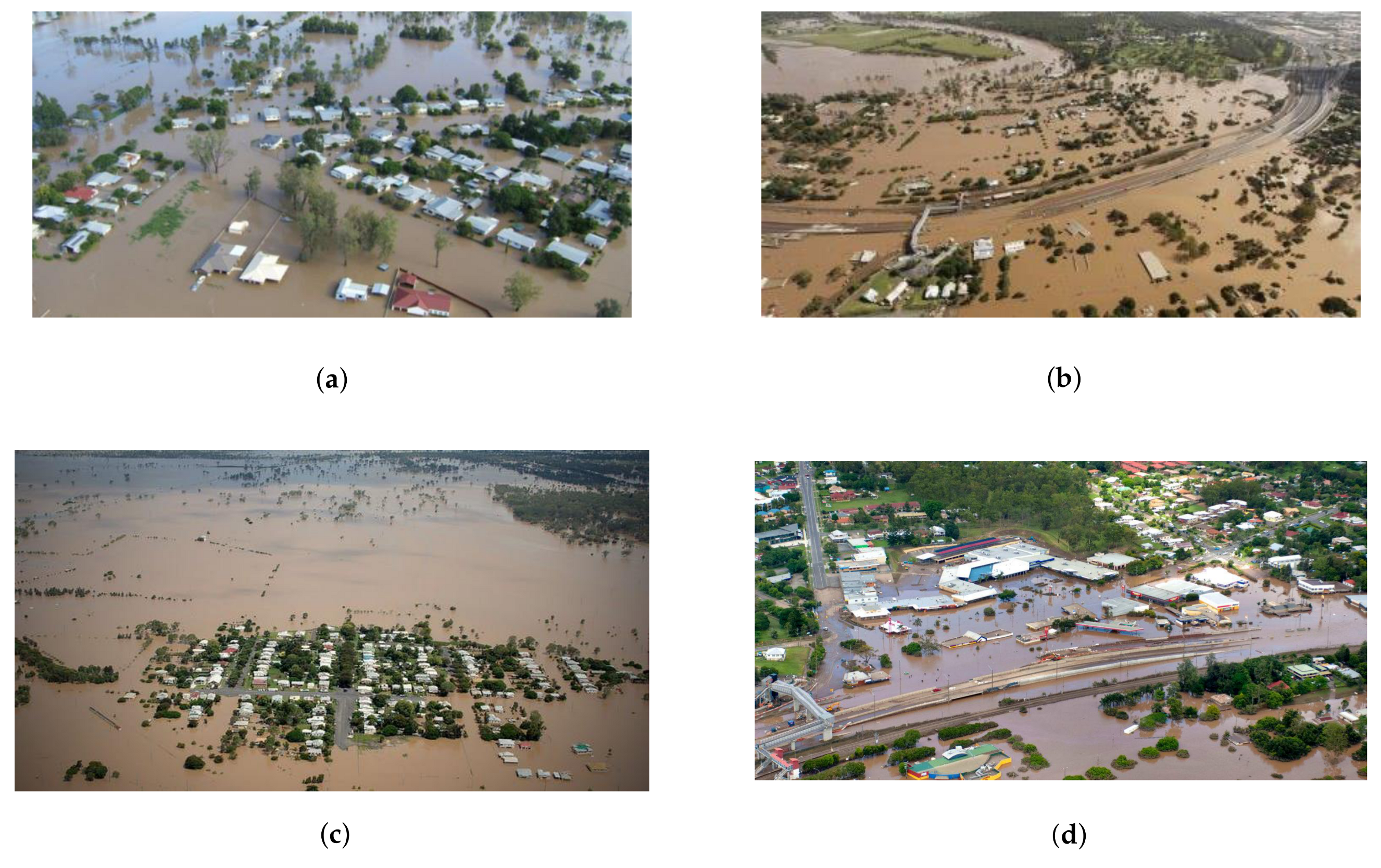
It is difficult to obtain a precise map of flooding extent as the extent of flood water during a flood event may change daily, and due to the adverse weather conditions during floods, it is difficult to acquire the ground truth data. There are few aerial field images obtained from the news archives as shown in Figure 3 display the extensive Queensland and New South Wales Flooding during 2011. However, considering the lack of ground truth data to evaluate the accuracy of the classification model, we considered to use published reference data as an approximated representation of the real flood extent that help to validate of our experiment. In a recent study conducted by Geoscience Australia [37], a comprehensive mapping of surface water for all of the Australia has been made for the first time. This involves analysis of temporal Landsat data covering the period of 1987–2014. The study has provided a series of confidence level maps of water presence covering Australia with a spatial resolution of 30 m. The water summary map was created by using a regression tree classification model. The aim of this web service is to develop a better understanding about where the waters are present throughout the years (permanent water features), where they are infrequently observed (intermittent water features), where flooding has been occasionally noticed and where there is no-water presence at all. The resultant water summary map was validated and filtered by using a number of independent variables from ancillary data. Probability scores were used as a predicted values of the independent factors. The ancillary dataset includes MrVBF (Multi-resolution Valley Bottom Flatness) product derived from the SRTM DSM (Shuttle Radar Topographic Mission Digital Surface Model), slope derived from the SRTM DSM, open water likelihood model-based surface water information across all of Australia from 1999 to 2010, The Australian hydrological features and the Australian statistical geography standard data [37]. The WOfS data achieves an overall accuracy of 97% with 93% correct identification of areas containing water [37]. The confidence percentage of water observation in pixels in the water summary dastaset has been utilized to get the labels for flood-water, permanent-water and non-water pixels.
2.1.3. Image Registration
We used Matlab Image Processing toolbox for performing the image registration. The second order polynomial geometric mapping transformation followed by control-point mapping function [42] were applied to implement the image registration process. The registration process helps to align each reference image with its corresponding Landsat image at pixel level which is required to generate the training samples. The 6 reflective channels/bands (visible bands: 1, 2 &3 and Infrared bands: 4, 5 & 7) were used for analysis.
We performed the similar image registration steps for Test images and the corresponding reference images obtained from the WOfS water confidence maps. After registration, we selected subsets of flooded areas from the Landsat Test images and used similar latitudinal and longitudinal extension to crop the corresponding areas from reference images.
2.1.4. Data Normalization
Minmax normalization was performed on geo-referenced images before adding them to the network. Normalization is a step of data pre-processing which is required in the field of data mining. This method helps to scale the values to fall within same specific ranges and may contribute to enhancing the accuracy of the machine learning algorithms like, artificial neural networks and clustering classifiers [43]. In our study, normalization helps to remove different range of of spectral reflectance values present in images.
2.1.5. Train, Validation and Test Sample Patches Generation for Model Design
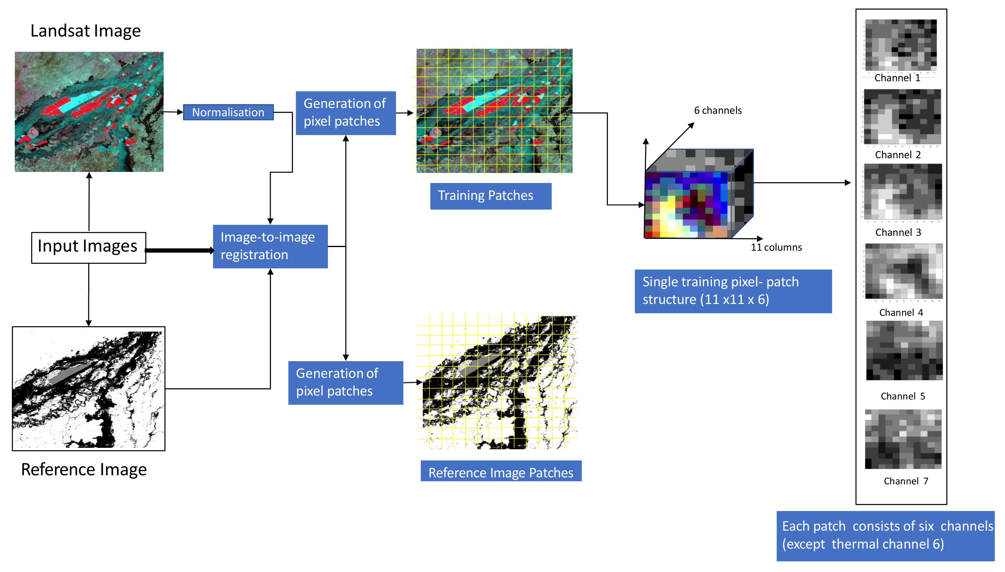
The Last step in stage-1 is to generate model’s input data of pixel-patches that were used to prepare train, validation and test sets and also assign the appropriate label to each sample. These sample-patches are utilised by the F-CNNs model during training process to obtain the underlying pattern in the training data [44]. This experiment considers spectral information from neighbouring pixels surrounded by the target-pixels into the classification process and to incorporate contextual information, so we chose small patches of pixels from the input images to generate the train and test sample sets. The class label of the pixel located at the centre of a patch was used as the class type for that particular patch. Pixels surrounding the centre pixel were used to determine the neighbouring area for information extraction. We generated eight different sets with varying neighbourhood sizes and preferred to apply odd numbers for the neighbourhood size to obtain a specific centre pixel location. Each training sample patch is generated based on a specific neighbourhood (N) size. Figure 4 displays the structure of a training sample extracted from Landsat data with N-11 size. Samples with N-1 size actually refers to single pixels used as samples. Model training with pixel-wise samples helped us to evaluate context-based classification performance with conventional pixel-wise classification process.
2.2. Stage 2: Model Building and Training
The second stage involves generation of train, validation and test sets, building the model architectures and training the models. Testing the performance of trained models on test set helped us to determine the optimum model architecture for the classification task.
2.2.1. Deep Network Structure
Convolution neural networks can be regarded as trainable feed-forward multi-layered artificial neural networks that comprise of multiple feature extraction stages [36,45]. Each of the feature extraction stage was consist of convolutional layers with learnable filters, pooling layers and activation functions or non-linearity layers [36].
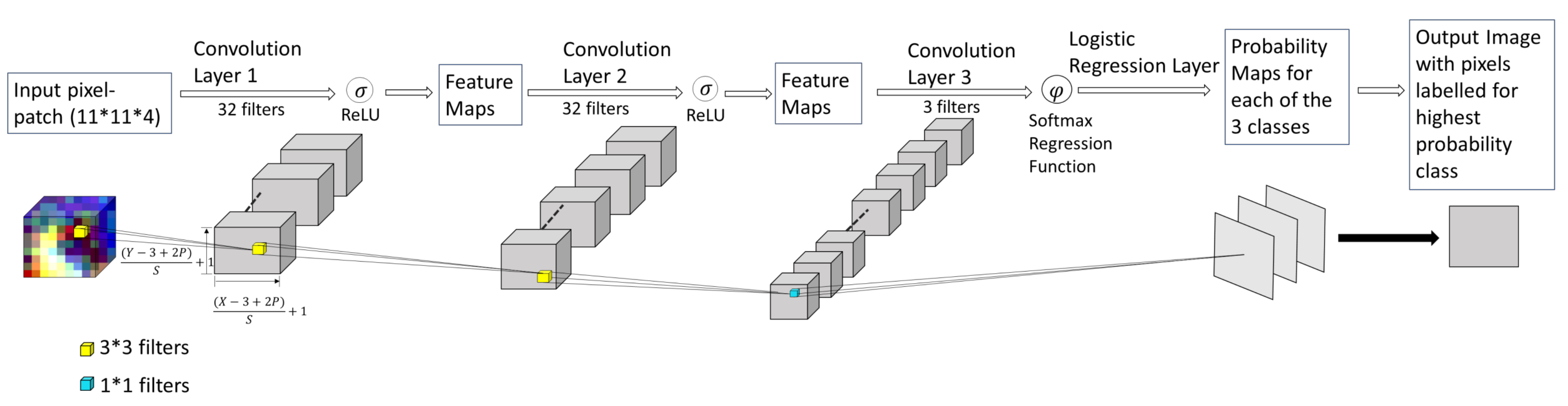
Our proposed fully convolutional neural networks (F-CNNs) consist of three convolutional layers. The training samples from Landsat images and their corresponding label image samples were uploaded to the proposed model network to train the model. Each layer applies a convolutional operation on the input image using learnable filters and passing the output feature maps to the next convolutional layer [36]. The first two convolutional layers (L1,L2) are designed using kernels (a set of learnable filters) of size 3 × 3. The dimensions of each filter allows the network to slide across the entire width and height of the local region and generates pixel-wise probabilities for each class based on the contextual information. The network takes pixel-patches (target pixel is at the centre of each patch) as input instead of single pixel. Filters of the last convolutional layers help the convolutional layer to learn patterns of the input training data of different class types. Each kernel gave the weight for each class label. Therefore, to keep the number of output feature maps of the last convolutional layer equal to the number of classes, the size of the filters in the last layer matched to the height and width of the input feature maps. The size () of the output feature maps generated by convolutional layers depends on the number of pooling and strides and the size of convolutional filters [46]. Assuming Y and X be the heights and width of the inputs to the convolutional layer, S be the stride and P be the padding, Equations (1) and (2) explain how the height and width of the outputs of each convolutional layer is determined.
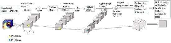
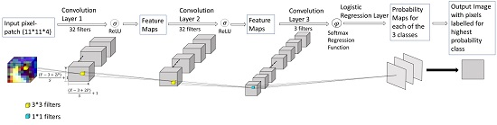
Figure 5 represents a F-CNNs model architecture using 32 filters of () size and each sample patch in the input data represents a () multidimensional matrix. Please refer Figure 6 for details about the dimension of input and output feature maps for the model illustrated in Figure 5.
We developed various designs of our proposed F-CNNs classification model by changing the number of filters used in each of the first two convolutional layers. The number of filters in each layer varies from 2 to 256 in powers of 2, and therefore, eight possible choices (2, 4, 8, 16, 32, 64, 128 and 256 filters) for each layer. In practice, that would lead to 64 possible permutations for (L1,L2).
In addition, with the aim of identifying the best neighbourhood size of training sample-patches for extracting contextual information using Landsat images, we experimented with 8 sets of training samples (one at a time) of eight different neighbourhood sizes (N), these are (N-1), (N-3), (N-5), (N-7), (N-9), (N-11), (N-13) and (N-23). Combined with 64 different choice of kernel numbers for L1 and L2, this would lead to (eight different training sets × 64 =) 512 possible variety of model architectures to test. Therefore, we reduced the number of combinations to make the process time permissible. We have used only eight combination filters between L1 and L2 by keeping the number of filters in both layers constant. As for example, considering number of filters is 64, both L1 and L2 layers use 64 filters for convolution. That results ( =) 64 different model architectures. The best performing model was selected from those possible 64 choices based on the training, validation and test performances. No zero-padding was used because the models in this experiment were designed to perform a classification task and hence, there is no need to preserve the spatial size of objects during training.
In deep neural networks, to reduce the dimensionality of the feature maps, pooling is introduced in between convolutional layers [45]. Due to the small size of network and small number of object categories (class types) using of pooling layers may cause loss of information by shrinking the size of the feature maps and therefore, we did not use any pooling layer in our proposed networks.
Activation functions is introduced to add the non-linearity to the networks. These functions help to decide whether the information received by the neuron is relevant or it should be discarded [36]. We used a Rectified Linear Unit or ReLU function after the first and second convolutional layers. We selected this function as it is used almost in every convolutional neural network models [36,47]. A softmax regression classification [48] function was used in the last convolution layer to estimate the probabilities for each class label in the input image. For each pixel, the class label with highest probability was determined as the final label of that pixel in the output image. The model was trained using categorical cross entropy loss function.
The total number of epochs/iterations was set to 2000. Although increasing the number of epochs may lead to improvements in training accuracy, we found that this number of epochs provided a good compromise between training time and accuracy. Stochastic gradient descent with Adam optimization algorithm was used by the model for fine tuning the hyper parameters. ADAM was developed by Diederik P. Kingma and Jimmy Lei Ba [49]. According to the authors, Adam is based on adaptive moment estimation [49]. The algorithm combines the advantages of AdaGrad and RMSProp optimization methods to deal with sparse gradients and noisy data respectively.
2.2.2. Training and Testing during Model Design
Training and test sets were prepared for each different neighbourhood size separately. Consequently, eight sets of training and test data were prepared for training the convolutional model. For each set, we consider a 90–10% ratio for dividing the input dastaset into train and test sets. The test set was not involved in the process of model training. This set was used to assess the classification performance of the trained model. The training set further were subdivided into train and validation set with a 80–20% ratio. Each training set covers a total of 4.50 million random selected samples (1.50 million training samples for each class type).
2.2.3. Validation during Model Design
A validation set is also required in this process which helps to assess the generalisation ability of the trained model on validation dastaset. If the validation performance is deteriorating while the training performance is improving over the epochs, the model assumes to be not well trained and has a very low generalisation ability. In deep learning terms it is called overfitting [44]. The training stage ended after 2000 iterations and finally the trained network was applied on test samples to generate classification outputs.
2.2.4. Selecting Best Performing Model
By investigating the training performances, we observe that in each combination-case the model achieved highest accuracy within the first 500 epochs and after that started overfitting. Therefore, we have only taken the training and validation performances for the first 500 epochs of the model for visualisation. Strong overfitting of the model using N-9, N-11, N-13 and N-23 training sets made us discard those four neighbourhood sizes for further investigations. By evaluating the test performance of the model to predict about the test samples helped us to determine the generalisation ability of the model and we were able to decide the optimum number of convolutional filters to be used in the model that performs best on Landsat data and the optimum size of the neighbourhood window for training sample patches.
2.3. Stage 3: Performing Classification and Error Estimation
The third and final stage of the methodology is to test the model over different Landsat images covering flood events across Australia. To compare the context-based F-CNNs classification performance with pixel-based conventional classification method, we chose the pixel-based SVM (support vector machines) classifier. SVM classifier was proposed by Vapnik [50]. SVM classifier works to find out the the optimum hyperplane to separate the class representative pixels from one class to another and mapped them.
We have calculated and analysed different validation coefficients from the confusion matrix to evaluate the performance of flood mapping. A confusion matrix is a matrix where N refers to the number of class labels being predicted. The coefficients include precision, recall and false negative rates.
To evaluate the model’s classification performances on each test images for detecting flooding extent we calculated the ‘precision’ (P) and the ‘Recall’ (R) values.The P index or positive predictive value of a particular class type refers to the percentages of correctly predicted positive cases among the total of the predicted positive cases. The R or hit rate measures the model sensitivity rate, that is it refers to the percentages of the positive cases that are correctly predicted by the model. To calculate the P and R from each classification result, we calculated the true positive (refers to pixels correctly classified as flood water), the false positive (refers to permanent water or non-flooded pixels erroneously classified as flood water) and the false negative (refers to flood water pixels that are missed) [51] from each classification output. The calculation of P and R are showin in Equations (3) and (4), respectively.
To have a comparative evaluation of the classification performance of context-based F-CNNs model with pixel-wise F-CNNs and SVM classifiers, we estimated the ‘overall accuracy’ (OA). The OA is estimated by dividing the total number of true positives or correctly classified pixels by the total number of classified pixels [52]. Assuming M be the total number of pixels in the error matrix or sum of row elements of the error matrix, be the sum of column elements or total number of accurately classified pixels and N be the total number of class types, the OA can be calculated as described in Equation (5) [53]. Moreover, to obtain a clear idea of the classification accuracy in detecting the extent of inundation we estimated the number of accurately predicted flooded pixels for context-based F-CNNs, pixel-wise F-CNNs and SVM classifiers.
3. Results
This section has two parts: first, we present the results of the training, validation and test performance during model design and the optimum model selection based on performance evaluation on validation and test dastasets. Secondly, we tested the optimal model to detect flooded extent using different Landsat images showing floods from different dates.
3.1. Training, Validation and Test Performances during the Model Design
Due to the space limitations we only report on the best performing models out of the possible 64. Figure 7 and Figure 8 list the training and validation performances of model networks with training sample sets of N-1, N-3, N-5 and N-7.
- (1)
- N-1 training samples are the representative of pixel-wise training samples and the graphs exhibit highest accuracy (80%) of the model on training and validation data using N-1 training samples with 2 learnable filters in the convolutional layers (the yellow and blue coloured curves in Figure 7a). Increase in the number of learnable convolutional filters results decrease in model’s accuracy of the model using N-1 data.
- (2)
- Graphs in Figure 7b shows that the model’s performance improves drastically with the highest level of accuracy increases to 92% using 32 learnable filters. But the overall performance of the F-CNNs model using N-1 sample set increases from 80% but compared to the performance of N-3, N-5 and N-7, moves down to the lowest accuracy (84%) level.
- (3)
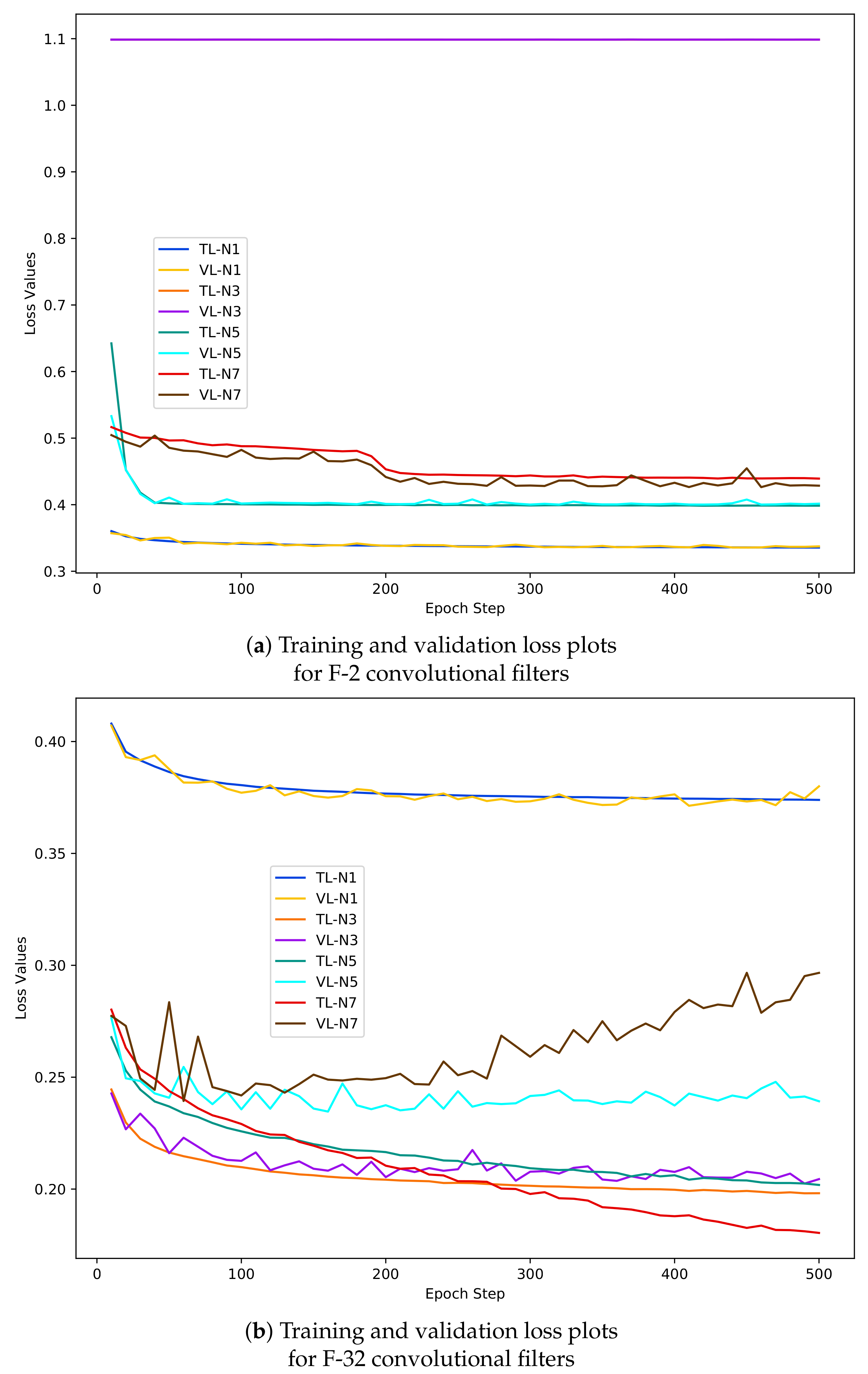
- The graphs in Figure 8 shows that the range of loss value remains constant (0.40–0.35) for N-1 training and validation data and the increase in filter numbers does not have any effect.
- (4)
- From the accuracy and loss graphs it can be outlined that the model performed with highest accuracy (95%) and lowest loss (0.20) values with N-3 samples (orange and violet coloured graph).
- (5)
- The F-CNNs model does not achieve the highest validation accuracy with N-5 and N-7 dastasets as we can see a deterioration of model’s validation performance compared to model’s training accuracy and loss results corresponds with N-5 (green and cyan coloured graphs) and N-7 (red and dark brown coloured graph) sample sets. For example, in Figure 8b the loss values recorded during model’s performance on N-7 validation dastaset (dark brown coloured graph) rises to 0.5 and shows a tendency of increasing at the 500th epoch where as the training loss (the red coloured curve) tends to decrease below 0.20. Similar trends can be observed for the accuracy graphs in Figure 7b.
Approximately, it required 24 h to perform the training process using High Performance Computing Server. We did not use GPU for the training process.
Overall, the analysis of the graphs of accuracy and loss plots reveals that the model is susceptible to ‘overfit’ or poor performance outside the training dastasets while increasing the neighbourhood size of sample patches. It is also evident that the model performs better both on training and validation data using context-based information than per-pixel information. On the whole, it can be seen that the model trained well using N-3 training sample patches and persistently performed well on validation dastaset.
Besides the training and validation performance evaluation, the evaluation of the F-CNNs performance of test sample patches have also done to decide the optimum model architecture. The main purpose of the evaluation of model’s performance on validation and test set was to choose the optimum model based on its generalisation ability [36]. The test accuracy and loss rates are listed in Table 2 and Table 3 respectively.
The observations from test performance evaluation are listed below:
- (1)
- Accuracy and loss test rates show that the F-CNNs model also performs worst while trained with N-1 sample set.
- (2)
- The F-CNNs model trained with N-3 sample patches performs best on the test samples with 32 learnable filters in first two feature extraction layers.
- (3)
- It is also evident that adding more filters to to the model with 32 learnable filters does not have any effect on model’s test performance proving that the model achieves its optimum level of performance. Therefore, we have finally selected 32 learnable filters as best choice for L1 and L2 convolutional layers and N-3 as best size of neighbourhood window for this study.
3.2. Evaluation of Classification Performance of the F-CNNs Model on Test Images
For classification test, instead of using the entire Landsat image scene, we selected a subset of the area covering locations of flooding. The test images were not a part of training the model networks. We selected six different Landsat image-subsets showing flood occurrences on different dates and locations for the quantitative assessment of classification performance. The details of the Landsat test images are listed in Table 4.
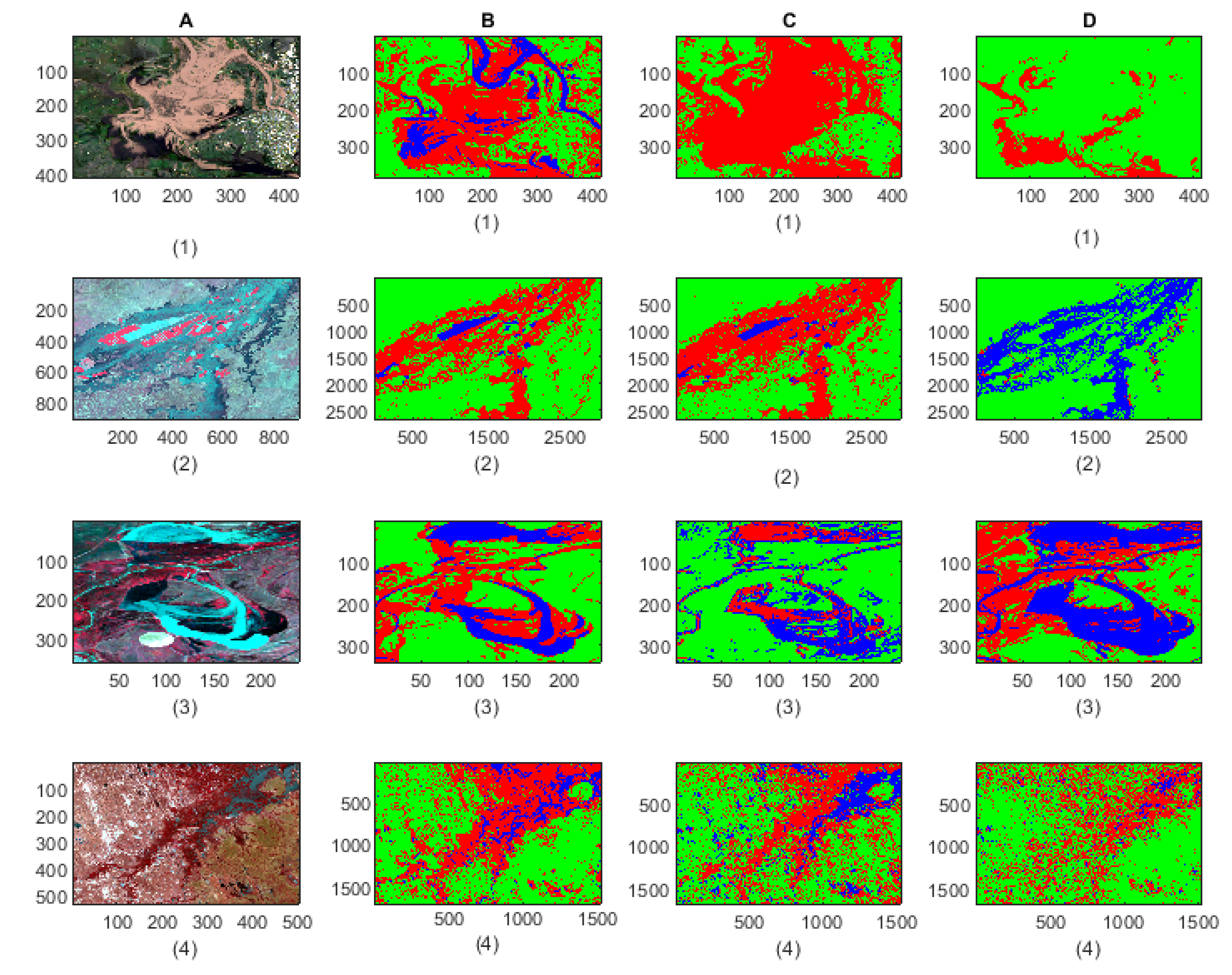
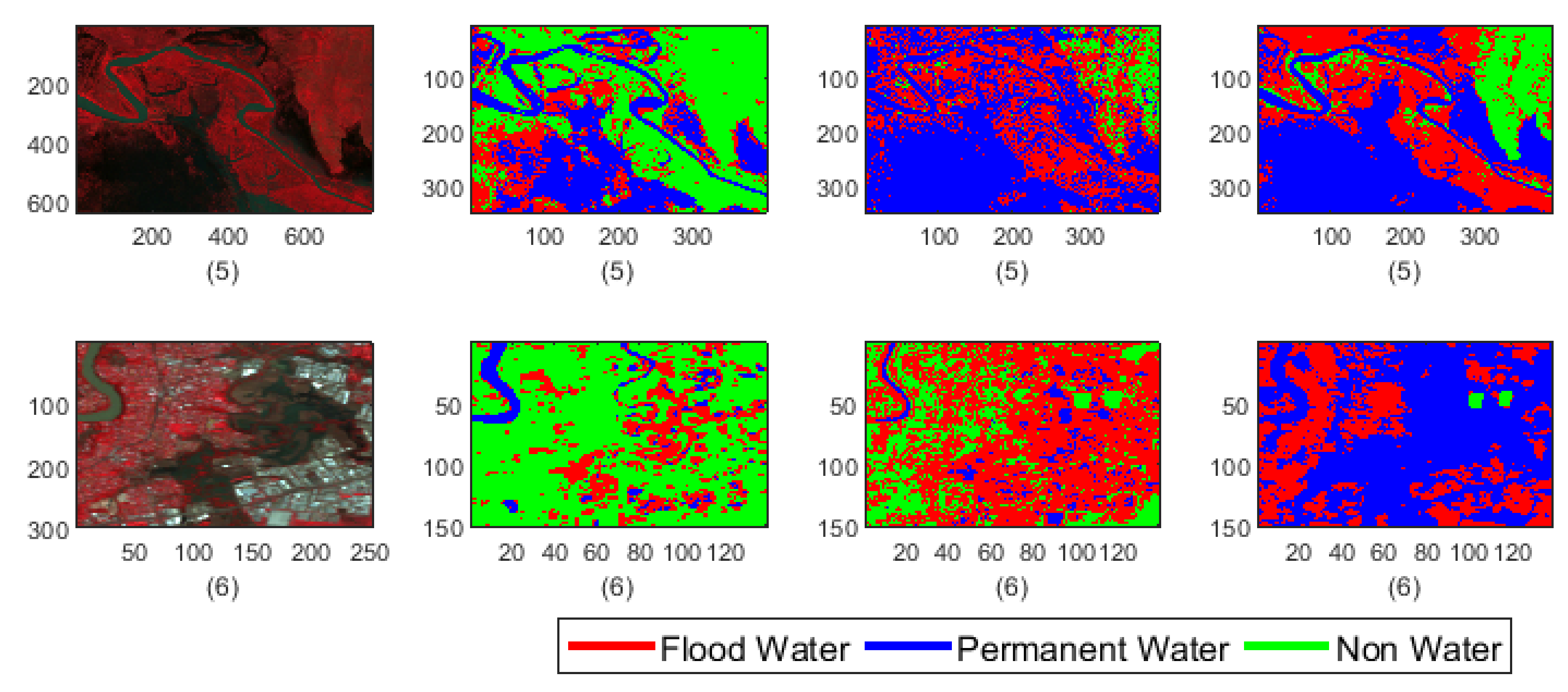
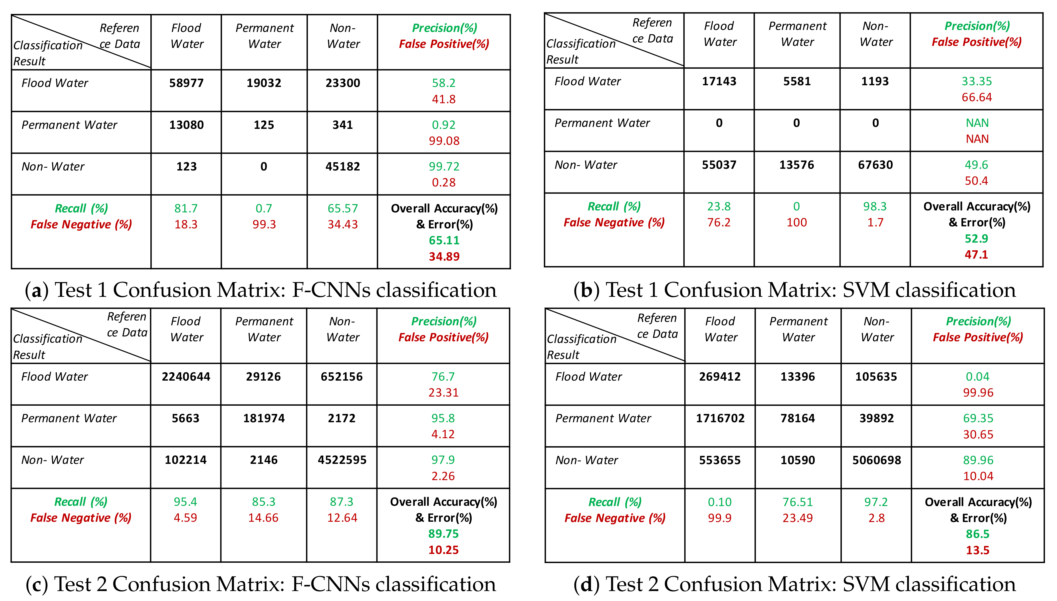
For the test image classification using the SVM, 1000 pixels from each class were randomly selected as the training samples. To match with the characteristics of the training samples of F-CNNs model, the training samples of the SVM classifier consists of normalised data and samples were collected from the Landsat images which used as input image in our proposed F-CNNs model. The mixture of spectral information from different images incorporates the spectral variation of class types in the training samples. The classification results are listed in Figure 9. The corresponding accuracy measures are listed in Figure 10 and Figure 11. By observing the classified images in Figure 9 few important points can be summarised:
- The classification results show that our proposed model is able to detect flood pixels compared to SVM classifier. The accuracy measures in Figure 10a for Test-1 shows that the recall rate of flood water class is 81.7% which means that the classification model able to detect 81.7% flooded pixels accurately. Compared to F-CNNs, the conventional SVM classification only detects 23.8% (Figure 10b) flood pixels accurately. Much of the flooded pixels are classified as land or non-water by SVM classifier which lowers down the precision rate of non-water class to 49.6%.
- Both the classification model fails to detect the permanent water from Test-1 image. While F-CNNs model detect permanent-water pixels as flood water (Figure 9(C-1)), SVM classifier misclassifies a considerable amount of flood water pixels and permanent water pixels (Figure 9(D-1)) as non-water class.
- The classification results (Figure 9(C-2,D-2)) of Test image-2 (Figure 9(A-2)) show that the F-CNNs model distinguishes between flood water and permanent water areas with 95.4% recall rate for flooded area detection (Figure 10c) while SVM classifier classifies the entire flooded areas as permanent water features and achieved as low as 0.10% recall rate (Figure 10d).
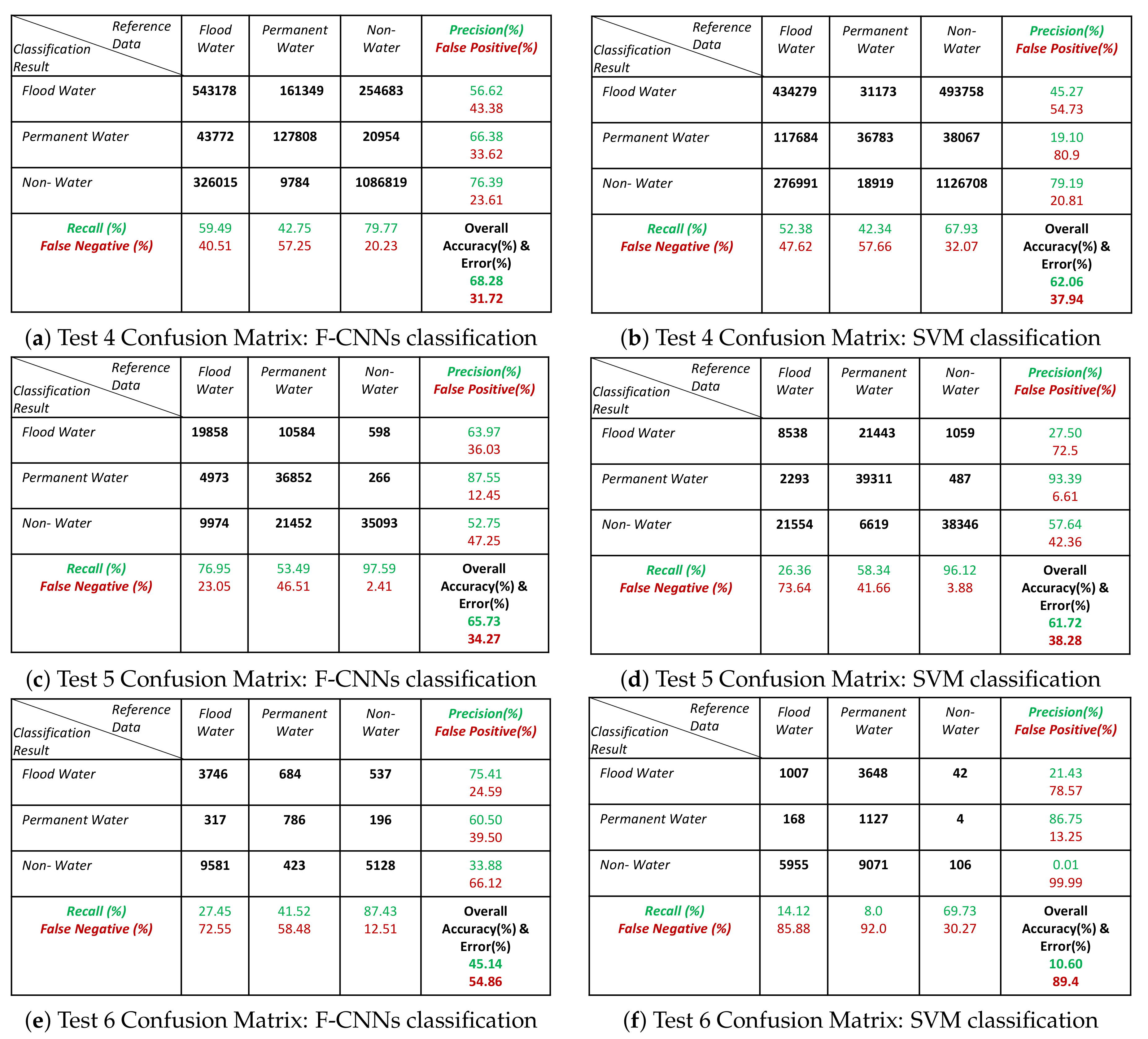
- Both the classification methods on Test-5 achieved with an overall accuracy less than 50%. However, the overall accuracies obtained by F-CNNs model ( 45.14%) is higher than the overall accuracy obtained by SVM classifiers (10.60%).
- However, the F-CNNs model does not able to achieve more than 70% overall accuracy level for every classification tasks, but it is clear from the results that the model is able to distinguish flood water from permanent-water features that the SVM classification method is not able to obtain as we observed in Figure 9(D-2) and Figure 9(D-6).
- Accuracy level of non-water area detection from all test images for both the classification method are showing more than 50% accurately classified pixels except for Test-6 where the SVM classification results show (Figure 9(D-6) and Figure 11f) all the non-water pixels are misclassified as flood waters.
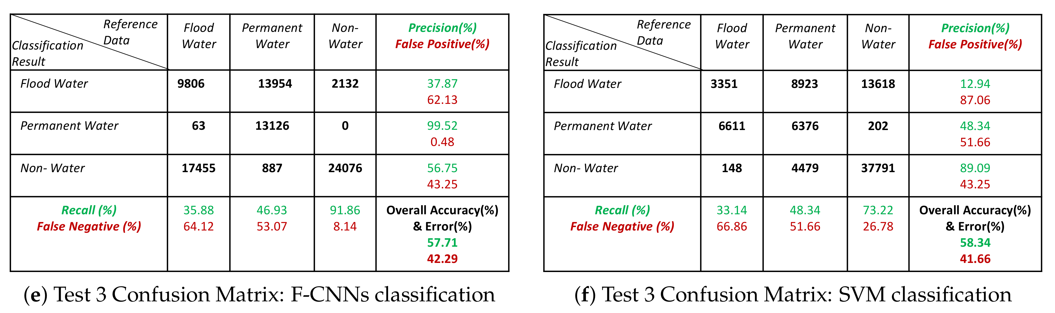
- The overall classification performance also show that F-CNNs model achieves classification accuracy higher than SVM classifiers except in case of Test- 3 classification performance where overall accuracies of both the classifiers are more or less similar (overall accuracy 57.71% for F-CNNs classifier and 58.34% for SVM classifier).
Finally, the processing time of the SVM classifier is also another important factor which makes the SVM classifier lagging behind the F-CNNs classification model. The processing time of SVM-classification method for test-1 and test-2 images are 0.45 h and 2.86 h and F-CNNs took 1.05 min and 3 min respectively. The experimental results and accuracy measures therefore, indicates that the application of neighbouring information with fully convolutional neural networks approach can be applied on a more generalised basis compared to conventional pixel-based classification methods. The model also able to distinguish between flood water and permanent water if there is enough spectral variability exists between these two class types.
4. Discussion
The aim of this paper is to propose a base-line architecture of a fully convolutional neural network classification model using neighbourhood pixel information for mapping the extent of flooded areas as well to distinguish flooded areas from permanent water bodies. In our knowledge, before no convolutional neural networks model was trained to map flooded areas by classifying multispectral images with more than 4-spectral bands. This approach was trained with a set of training samples collected from different images covering flood water, permanent water and non-water training samples. The trained model was applied on six different Landsat flood images of Australia and these test data are independent to the training set. To compare the performance of the proposed model we also used the conventional SVM classification method to classify those test images. For comparison purpose we selected a random sample of 1000 pixels for each of the class types from the similar input images that we used for training sample selection of F-CNNs classification model.
The training, test and validation experiments for model design determined optimal model architecture with 32 learnable convolutional filters or the classification purpose. The evaluation of model’s performance on validation and test set also determined the optimal neighbourhood size of training sample patches to pixels.
The F-CNNs classification method obtains higher overall accuracies compared to SVM classifier on test images except Test- 3 where accuracies obtained from both the classifiers are almost equal (57.71% for F-CNNs classifier and 58.34% for SVM classifier). When focusing on detecting the extent of flooding, it can be stated that our proposed model is able to detect flooded areas more accurately than by the SVM method as, we have observed that for test image-1 about 81.7% of flood water pixels are successfully retrieved by the F-CNNs model compared to only 23.8% by the SVM classification model.
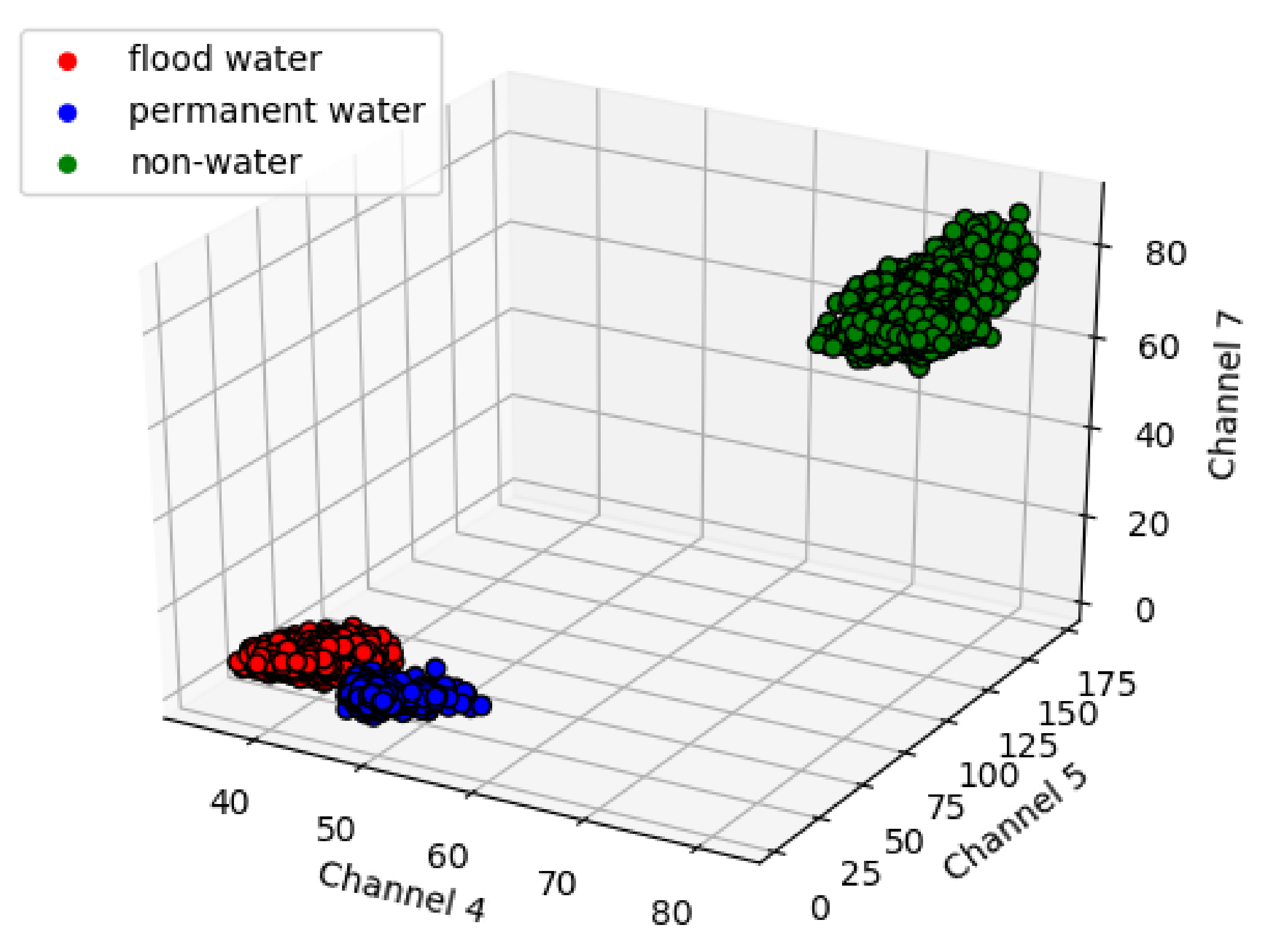
Our proposed method also shown to be able to distinguish flooded area and permanent water areas with 95.4% and 85.3% of detection rate for flood water and permanent water bodies respectively. However, from the classification results it is evident that the method is dependent on the distinctive spectral properties of those two class types. As we can observe in the classification results of test image-1 (Figure 9a) that due to the turbid color of the river and the flooded area the F-CNNs model misclassified the permanent water bodies as flood. To examine the spectral distinctiveness of flood water and permanent water class, a feature space plot was generated by using few randomly selected samples of flood water and permanent water class from Test image-1. It is an established fact that the spectral characteristics are more distinctive for water features in the infrared wavelength region and beyond [52]. Therefore, few randomly collected class samples of channel-4, channel-5 and channel-7 (infrared bands) were selected from the Test image-1 and plotted on a 3D graph plot in Figure 12. The graph clearly shows that the flood water and the permanent water samples are overlapping with each other in the infra-red spectrum region.
Therefore, incorporating spectral properties are not enough to separate these two features and to overcome this issue further research work includes ancillary data like altitude information from SRTM Digital Elevation Model into the classification process.
Additionally, from the accuracy measures in Figure 9 it is also observed that the model may have a tendency to falsely classified the non-water pixels as flood water due to the similar spectral similarity but the percentages of such miss classification is very less for F-CNNs model.
In Australia, flooding is the most frequently occurring natural hazards which affects the community. The problem of flooding is critical in Queensland and New South Wales as every year these two states experience a series of scattered flooding events [54]. It is therefore, important to obtain a flooding extent map during real-time flood events. The Australian disaster management organisations relies on different classification, hydrologic and hydraulic models for detecting flooded areas. Generally, the selection of using a model depends on data availability [55]. Long processing time and computational efficiency is required to obtain flooding extent by using conventional machine learning methods which is not desirable during the flooding emergency. Our aim therefore to propose a model that can be able to produce flood maps with minimum required time and using data that are freely accessible. Moreover, due to the lack of generalisation ability the conventional machine learning classifiers are required to be retrained before using on a new flooding image to detect the extent of inundation. Compared to the conventional classification methods, our proposed methods are more generalised in nature and therefore, able to detect flooded areas from freely available Landsat images as we have already shown in our test experiments. The classification F-CNNs classification model requires minimum processing time which is sometime less than a minutes using a desktop computer with 64-bit operating systems and 16 GB RAM. The software (latest JetBrains PyCharm Community Edition) required to run the classifier is also freely available to download. Our proposed model does not require any permanent water mask image to separate the permanent water bodies from flooded areas. Therefore, we believe that our proposed method is able to provide a solution to obtain rapid flood extent maps for an efficient relief work. Our propose context-based optimal convolutional neural networks model with 32 learnable filters in each layer is a base model and therefore, does not able to produce high accuracy for every test experiments but definitely showing more accurate classification compared to conventional classification methods that are based on single spectral information. We are currently working on the application of elevation data with the spectral information to detect the class types more accurately as well as to detect flooded areas obscured by clouds or vegetation cover.
5. Conclusions
This study presents a novel approach of using neighbourhood information of pixel spectral properties into an advanced machine learning model with optimal architectural design for mapping the flooding extent from multispectral Landsat images. Our study also addresses the problem of separating flood water from permanent water features which has not been investigated in flood mapping [35,36]. In this paper, we prepare a base-line fully convolutional neural network model (F-CNNs) to perform the classification method. To obtain the best performing model, we investigated the architecture design by changing the number of convolutional filters used in the first two convolutional layers. In this study, we have also investigated the effectiveness of different sizes of training neighbourhood windows for incorporating the contextual information to train the classification model. The FCNNs model performed best with 32 learnable filters and it is observed that size of neighbourhood sample patches is ideal for using the F-CNNs model on Landsat images.
To evaluate the performance the F-CNNs model by comparing with the performance of traditional pixel-based classification methods, we choose the conventional pixel-based support vector machines on the test images. The classification results shows that our proposed model was able to detect flooded areas and separate flood water features from permanent water features; however, the accuracy varies depending upon distinguishable spectral information present in the test image. For images with almost similar spectral characteristics of flood and permanent water features, the model misclassified permanent water pixels as flood water. However, overall, the experimental results showed that the F-CNNs model is more efficient to map flood extent areas with a recall rate of more than 70% in few test experiments compared to the conventional SVM classification results with less than 30% recall rate for flooded area detection. The accuracy of measures also proved that the F-CNNs model can be applied to extract flooded areas from any Landsat images covering floods in Australia due to its generalisation ability.
Further research work involves: 1. Using the elevation information from the SRTM DEM to define rules to separate flood water from permanent water features; 2. Incorporation of the DEM image into the classification process to refine the prior probability generated by the F-CNNs model and in this way the misclassified pixels or false positives can be correctly labelled; and 3. The method also helps to detect flooded areas obscured by cloud cover and vegetation cover. Finally, we also aim to test this model in artificially created images covering different possible situations based on real-time flood scenarios and in the current results to refine the labels of the misclassified pixels.
Author Contributions
C.S. conceived, designed, performed the experiments and wrote this study; F.M. guided the model design; A.W. helped to access the images; L.M. helped organized the paper; C.S., L.M., F.M. and A.W. analyzed the experimental results and contribute with the manuscript writing.
Funding
This research received no external funding. The APC was funded by the Queensland University of Technology.
Acknowledgments
The authors would like to thank Norman Mueller (Earth Observation Scientist, Geosciences Australia) for providing us the access to Water Summary dastaset. All Landsat-5 TM data are distributed by the Land Processes Distributed Active Archive Center (LP DAAC), located at USGS/EROS, Sioux Falls, SD. Available online: http://lpdaac.usgs.gov. The High Performance Computing (HPC) lab of Queensland University of Technology has been utilized to run the experimental work on training data preparation and F-CNNs model training.
Conflicts of Interest
The authors declare no conflicts of interest.
References
- DNRM. Flood-Ready Queensland- Queensland Flood Mapping Program: Flood Mapping Implementation Kit. Available online: https://www.dnrm.qld.gov.au/__data/assets/pdf_file/0009/230778/flood-mapping-kit.pdf (accessed on 5 March 2018).
- Klemas, V. Remote Sensing of Floods and Flood-Prone Areas: An Overview. J. Coaster Res. 2015, 31, 1005–1013. [Google Scholar] [CrossRef]
- Zazo, S.; Rodríguez-Gonzálvez, P.; Molina, J.L.; González-Aguilera, D.; Agudelo-Ruiz, C.A.; Hernández-López, D. Flood hazard assessment supported by reduced cost aerial precision photogrammetry. Remote Sens. 2018, 10, 1566. [Google Scholar] [CrossRef]
- Liu, X.; Sahli, H.; Meng, Y.; Huang, Q.; Lin, L. Flood inundation mapping from optical satellite images using spatiotemporal context learning and modest AdaBoost. Remote Sens. 2017, 9, 617. [Google Scholar] [CrossRef]
- Ortega-Terol, D.; Moreno, M.; Hernández-López, D.; Rodríguez-Gonzálvez, P. Survey and classification of large woody debris (LWD) in streams using generated low-cost geomatic products. Remote Sens. 2014, 6, 11770–11790. [Google Scholar] [CrossRef]
- Rahman, M.R.; Thakur, P. Detecting, mapping and analysing of flood water propagation using synthetic aperture radar (SAR) satellite data and GIS: A case study from the Kendrapara District of Orissa State of India. Egyptial J. Remote. Sens. Space Sci. 2018, 21, S37–S41. [Google Scholar] [CrossRef]
- Feng, Q.; Gong, J.; Liu, J.; Li, Y. Flood mapping based on multiple endmember spectral mixture analysis and random forest classifier- the case of Yuyao, China. Remote Sens. 2015, 7, 12539–12562. [Google Scholar] [CrossRef]
- Faghih, M.; Mirzaei, M.; Adamowski, J.; Lee, J.; El-Shafie, A. Uncertainty estimation in flood inundation mapping: An application of non-parametric bootstrapping. River Res. Appl. 2017, 33, 611–619. [Google Scholar] [CrossRef]
- Zhao, J.; Zhong, Y.; Shu, H.; Zhang, L. High-resolution image classification integrating spectral-spatial- location cues by conditional random fields. IEEE Trans. Image Process. 2016, 25, 4033–4045. [Google Scholar] [CrossRef]
- Isikdogan, F.; Bovik, A.; Passalacqua, P. Surface water mapping by deep learning. IEEE J. Sel. Topics Appl. Earth Obs. Remote. Sens. 2017, 10, 4909–4918. [Google Scholar] [CrossRef]
- Ogashawara, I.; Curtarelli, M.; Ferreira, C. The use of optical remote sensing for mapping flooded areas. J. Eng. Res. Appl. 2013, 3, 1956–1960. [Google Scholar]
- Du, Y.; Zhang, Y.; Ling, F.; Wang, Q.; Li, W.; Li, X. Water bodies’ mapping from Sentinal-2 imagery with modified normalized difference water index at 10-m spatial resolution produced by sharpening the SWIR band. Remote Sens. 2016, 8, 354. [Google Scholar] [CrossRef]
- Amarnath, G. An algorithm for rapid flood uinundation mapping from optical data using a reflectance differencing technique. J. Flood Risk Manag. 2014, 7, 239–250. [Google Scholar] [CrossRef]
- Huang, C.; Chen, Y.; Wu, J. Mapping spatio-temporal flood inundation dynamics at large river basin scale using time-series flow data and MODIS imagery. Int. J. Appl. Earth Onservation Geoinform. 2014, 26, 350–362. [Google Scholar] [CrossRef]
- Haq, M.; Akhtar, M.; Muhammad, S.; Paras, S.; Rahmatullah, J. Techniques of remote sensing and gis for flood monitoring and damage assessment: A case study of Sindh province, Pakistan. Egypt. J. Remote Sens. Space Sci. 2012, 15, 135–141. [Google Scholar] [CrossRef]
- Villa, P.; Gianinetto, M. Monsoon flooding response: A multi-scale approach to water-extent change detection. In Proceedings of the ISPRS Commission VII Mid-term Symposium Remote Sensing: From Pixels to Processes, Enschede, The Netherlands, 8–11 May 2006; pp. 1–6. [Google Scholar]
- Chignell, S.; Anderson, R.; Evangelista, P.; Laituri, M.; Merritt, D. Multi-temporal independent component analysis and Landsat 8 for delineating maximum extent of the 2013 Colorado Front Range flood. Remote Sens. 2015, 7, 9822–9843. [Google Scholar] [CrossRef]
- Pierdicca, N.; Pulvirenti, L.; Chini, M.; Guerriero, L.; Candela, L. Observing floods from space: Experience gained from cosmo-skymed observations. Acta Astronaut 2013, 84, 122–133. [Google Scholar] [CrossRef]
- Nandi, I.; Srivastava, P.; Shah, K. Floodplain mapping through support vector machine and optical/infrared images from Landsat 8 OLI/TIRS sensors: Case study from Varanasi. Water Resour. Manag. 2017, 31, 1157–1171. [Google Scholar] [CrossRef]
- Kia, M.B.; Pirasteh, S.; Pradhan, B.; Mahmud, A.; Sulaiman, W.; Moradi, A. A artificial neural network model for flood simulation using GIS: Johor River Basin, Malaysia. Environ. Earth Sci. 2012, 67, 251–264. [Google Scholar] [CrossRef]
- Malinowski, R.; Groom, G.; Schwanghart, W.; Heckrath, G. Detection and delineation of localized flooding from WorldView-2 Multispectral Data. Remote Sens. 2015, 7, 14853–14875. [Google Scholar] [CrossRef]
- Richards, J.; Jia, X. Remote Sensing Digital Image Analysis: An Introduction; Springer: Berlin/Heidelberg, Germany, 2006. [Google Scholar]
- Bangira, T.; Alfieri, S.; Menenti, M.; Van Niekerk, A.; Vekerdy, Z. A spectral unmixing method with ensemble estimation of endmembers: Application to flood mapping in the Caprivi floodplain. Remote Sens. 2017, 9, 1013. [Google Scholar] [CrossRef]
- Gomez-Palacios, D.; Torres, M.; Reinoso, E. Flood mapping through principal component analysis of multitemporal satellite imagery considering the alteration of water spectral properties due to turbidity conditions. Geomat. Nat. Hazards Risk 2017, 8, 607–623. [Google Scholar] [CrossRef]
- Bui, D.; Hoang, N.D. A Bayesian framework based on a Gaussian mixture model and radial-basis-function Fisher discriminant analysis (BayGmmKda VI.1) for spatial prediction of floods. Geosci. Model Dev. 2017, 10, 3391–3409. [Google Scholar]
- Dey, C.; Jia, X.; Fraser, D.; Wang, L. Mixed pixel analysis for flood mapping using extended support vector machine. In 2009 Digital Image Computing: Techniques and Applications; IEEE: Melbourne, Australia, 2009; pp. 291–295. [Google Scholar]
- Wang, L.; Jia, X. Integration of soft and hard classifications using extended support vector machines. IEEE Geosci. Remote Sens. Lett. 2009, 6, 543–547. [Google Scholar] [CrossRef]
- Sarker, C.; Mejias, L.; Woodley, A. Integrating recursive Bayesian estimation with support vector machine to map probability of flooding from multispectral Landsat data. In Proceedings of the 2016 International Conference on Digital Image Computing: Techniques and Applications (DICTA), Gold Coast, Australia, 30 November–2 December 2016; pp. 1–8. [Google Scholar]
- Dao, P.; Liou, Y. Object-oriented approach of Landsat Imagery for flood mapping. Int. J. Comput. Appl. 2015, 7, 5077–5097. [Google Scholar]
- Pulvirenti, L.; Chini, M.; Pierdicca, N.; Guerriero, L.; Ferrazzoli, P. Flood monitoring using multi-temporal COSMO-SkyMed data: Image segmentation and signature interpretation. Remote Sens. Environ. 2011, 115, 990–1002. [Google Scholar] [CrossRef]
- Huang, C.; Townshend, J.; Liang, S.; Kalluri, S.; DeFries, R. Impact of sensor’s point spread function on land cover characterization: Assessment and deconvolution. Remote Sens. Environ. 2002, 80, 203–212. [Google Scholar] [CrossRef]
- Gurney, C.M. The use of contextual information in the classification of remotely sensed data. Photogramm. Eng. Remote Sens. 1983, 49, 55–64. [Google Scholar]
- Moggiori, E.; Tarabalka, Y.; Charpiat, G.; Alliez, P. Convolutional neural networks for large-scale remote sensing image classification. IEEE Trans. Geosci. Remote Sens. 2017, 55, 645–657. [Google Scholar] [CrossRef]
- Amit, S.; Aoki, Y. Disaster detection from aerial imagery with convolutional neural network. In Proceedings of the International Electronics Symposium on Knowledge Creation and Intelligent Computing, (IES-KCIC), Surabaya, Indonesia, 26–27 September 2017; pp. 1–7. [Google Scholar]
- Nogueira, K.; Fadel, S.G.; Dourado, Í.C.; Werneck, R.d.O.; Muñoz, J.A.V.; Penatti, O.A.B.; Calumby, R.T.; Li, L.T.; dos Santos, J.A.; Torres, R.d.S. Exploiting convNet diversity for flooding identification. IEEE Geosci. Remote Sens. Lett. 2018, 15, 1446–1450. [Google Scholar] [CrossRef]
- Gebrehiwot, A.; Hashemi-Beni, L.; Thompson, G.; Kordjamshidi, P.; Langan, T. Deep convolution neural network for flood extent mapping using unmanned aerial vehicles data. Sensors 2019, 19, 1486. [Google Scholar] [CrossRef]
- Mueller, N.; Lewis, A.; Roberts, D.; Ring, S.; Melrose, R.; Sixsmith, J.; Lymburner, L.; McIntyre, A.; Tan, P.; Curnow, S.; et al. Water observations from space: Mapping surface water from 25 years of Landsat imagery across Australia. Remote Sens. Environ. 2016, 174, 341–352. [Google Scholar] [CrossRef]
- Timms, P. Warmer Ocean Temperatures Worsened Queensland’s Deadly 2011 Floods: Study. 2015. Available online: https://www.abc.net.au/news/2015-12-01/warmer-ocean-temperatures-worsened-queenslands-2011-flood-study/6989846 (accessed on 18 March 2017).
- Croke, J. Extreme Flooding Could Return in South-East Queensland. 2017. Available online: https://www.uq.edu.au/news/article/2017/01/extreme-flooding-could-return-south-east-queensland (accessed on 18 March 2017).
- Coates, L. Moving Grantham? Relocating Flood-Prone Towns Is Nothing New. 2012. Available online: https://theconversation.com/moving-grantham-relocating-flood-prone-towns-is-nothing-new-4878 (accessed on 18 March 2017).
- Roebuck, A. Queensland Floodplain Management Plan Sets New National Benchmark. 2019. Available online: http://statements.qld.gov.au/Statement/2019/4/9/queensland-floodplain-management-plan-sets-new-national-benchmark (accessed on 29 September 2017).
- Mathworks. Control Point Registration. Available online: https://au.mathworks.com/help/images/control-point626registration.htm (accessed on 13 June 2019).
- Shalabi, A.L.; Shaaban, Z.; Kasasbeh, B. Data Mining: A preprocessing Engine. J. Comput. Sci. 2005, 2, 735–739. [Google Scholar] [CrossRef]
- Rosebroke, D. Understanding convolutions. In Deep Learning for Computer Vision with Python:Starter Bundle, 2nd ed.; PyImageSearch.com: USA, 2018; Available online: https://www.pyimagesearch.com/deep-learning-computer-vision-python-book (accessed on 16 July 2019).
- Kim, P. Convolutional neural network. In Matlab Deep Learning: With Machine Learning, Neural 616 Networks and Artificial Intelligence; Apress: New York, NY, USA, 2017; Chapter 6. [Google Scholar]
- Andrej, K. CS231n: Convolutional Neural Networks for Visual Recognition. 2016. Available online: http://cs231n.github.io/convolutional-networks/ (accessed on 20 August 2019).
- Simonyan, K.; Zisserman, A. Very deep convolutional networks for large-scale image recognition. In Proceedings of the International Conference on Learning Representations, San Diego, CA, USA, 7–9 May 2015. [Google Scholar]
- Liu, S.; McGree, J.; Ge, Z.; Xie, Y. 4- Computer Vision in Big Data Applications; Academic Press: San Diego, CA, USA, 2016. [Google Scholar]
- Kingma, D.; Lei Ba, J. ADAM: A method for stochastic optimization. In Proceedings of the 3rd International Conference for Learning Representations, San Diego, CA, USA, 7–9 May 2015. [Google Scholar]
- Vapnik, V. The Nature oif Statistical Learning Theory; Springer: New York, NY, USA, 1995. [Google Scholar]
- Notti, D.; Giordan, D.; Caló, F.; Pepe, A.; Zucca, F.; Pedro Galve, J. Potential and Limitations of Open Satellite Data for Flood Mapping. Remote Sens. 2018, 10, 1673. [Google Scholar] [CrossRef]
- Lillesand, T.; Kiefer, R.; Chipman, J. Energy interactions with earth surface features. In Remote Sensing and Image Interpretation; John Wiley and Sons, Inc.: Hoboken, NJ, USA, 2008. [Google Scholar]
- Jensen, J. Remote sensing-derived thematic map accuracy assessment. In Introductory Digital Image Processing: A Remote Sensing Perspective, 4th ed.; Pearson Education, Inc.: Glenview, IL, USA, 2004; pp. 570–571. [Google Scholar]
- Keys, C. Towards Better Practice: The Evolution Of Flood Management in New South Wales; Technical Report; New South Wales State Emergency Services: New South Wales, Australia, 1999. [Google Scholar]
- BMT WBM Pty Ltd. Guide for Flood Studies and Mapping in Queensland; Technical Report; Department of Natural Resources and Mines: Queensland, Australia, 2017. [Google Scholar]
Figure 1.
An overview of the stages of our proposed method of flood mapping.

Figure 2.
Footprints of the selected Landsat-5 TM images: A single band (Band-5) of each selected Landsat-5 images is overlaid on the Google Earth map based on their location.
Figure 2.
Footprints of the selected Landsat-5 TM images: A single band (Band-5) of each selected Landsat-5 images is overlaid on the Google Earth map based on their location.

Figure 3.
Aerial Images from different sources showing different flood affected regions of Queensland and NSW Flood, 2011. (a) Southern Queensland town of Theodore during 2011 floods [38]. Photo was taken by Jackie Jewell; (b) State Library of Queensland during 2011 floods [39]; (c) Lockyer Valley Region, Queensland, Australia during 2011 floods [40]; (d) Brisbane River flooding at Goodna during 2011 floods [41].

Figure 4.
The workflow for the generation of a training sample. Geometric correction and data normalisation is followed by generation of training sample patches. For training samples with neighbourhood size (N-11), each training sample consists of 11 rows, 11 columns and six channels or bands (Channel 1, 2 and 3 represents red, green and blue; channel 4 represents near-infra red, channel 5 represents middle-infrared and channel 6 represents short-wave infra-red).

Figure 5.
Overview of the proposed Fully Convolutional Neural Network architecture. The neural network consist of three convolutional layers. First two convolutional layers contain 32 filters each with size each. The last layer replaces the fully connected layer with a convolutional layer containing three filters with size and a softmax regression function to obtain class label probability for each pixel.

Figure 6.
Overview of the process flow for an architecture with (L1,L2) = (32,32) trained with N-11. Filters and feature maps are shown as well as input and output data sizes at each layer.
Figure 6.
Overview of the process flow for an architecture with (L1,L2) = (32,32) trained with N-11. Filters and feature maps are shown as well as input and output data sizes at each layer.

Figure 7.
Training and validation accuracy plots of model networks with combinations of different numbers of convolutional filter and different sets of training sample. The number of learnable filters used to the model is specified as ‘F-number’ in every sub-caption. TA and VA in legends denote training accuracy and validation accuracy.

Figure 8.
Training and validation loss plots of model networks with combinations of different numbers of convolutional filter and different sets of training sample. The number of learnable filters used to the model is specified as ‘F-number’ in every sub-caption. TL and VL in legends denote training loss and validation loss. Neighbourhood size is depicted as (N).

Figure 9.
Classification results of F-CNNs and SVM classification models. Cells-(A1–A6) showing the original Landsat test images. Cells-(B1–B6) showing the labelled images from the reference data. Cells-(C1–C6) showing the classification results of context-based F-CNNs model. Cells-(D1–D6) showing the classification results of pixel-based SVM model.


Figure 10.
Confusion matrices of Test image 1, Test image 2 and Test image 3 classification results by F-CNNs and SVM: Confusion matrix listed the accuracy measures.
Figure 10.
Confusion matrices of Test image 1, Test image 2 and Test image 3 classification results by F-CNNs and SVM: Confusion matrix listed the accuracy measures.


Figure 11.
Confusion matrices of Test image 4, Test image 5 and Test image 6 classification results by F-CNNs and SVM: Confusion matrix listed the accuracy measures.
Figure 11.
Confusion matrices of Test image 4, Test image 5 and Test image 6 classification results by F-CNNs and SVM: Confusion matrix listed the accuracy measures.

Figure 12.
The scatter plot of class samples from test image-1 on a 3D graph. The axis represents channel-4, channel-5 and channel-7. The graph shows that even in the infrared region the spectral properties of flood water and permanent water are overlapping.
Figure 12.
The scatter plot of class samples from test image-1 on a 3D graph. The axis represents channel-4, channel-5 and channel-7. The graph shows that even in the infrared region the spectral properties of flood water and permanent water are overlapping.


Table 1.
Landsat-5 Thematic Mapper Image Specification.
| Specification | Description |
|---|---|
| Revisit Time | 16 Days |
| Spatial Resolutions | 30 m (Reflective bands) 120 m (thermal band) |
| Spectral Channels/Bands | Reflective bands: 1. Visible Blue (0.45–0.52 m); 2. Visible Green (0.52–0.60 m); 3. Visible Red (0.63–0.69 m); 4. Near Infrared (0.76–0.90 m); 5. Short wave Infrared (1.55–1.75 m); 7. Mid Infrared (2.08–2.35 m) Thermal band: 6. Thermal (10.40–12.50 m) |
| Scene Size (Size of an image) | 170 km × 185 km |
| Sensors | Thematic Mapper |
Table 2.
Accuracy Rate of model networks using various number of learnable filters on N-3, N-5 and N-7 dastaset.
Table 2.
Accuracy Rate of model networks using various number of learnable filters on N-3, N-5 and N-7 dastaset.
| Filter No. | N-1 Test Accuracy | N-3 Test Accuracy | N-5 Test Accuracy | N-7 Test Accuracy |
|---|---|---|---|---|
| 2 | 0.61 | 0.33 | 0.86 | 0.86 |
| 4 | 0.80 | 0.88 | 0.87 | 0.88 |
| 8 | 0.74 | 0.91 | 0.89 | 0.89 |
| 16 | 0.73 | 0.91 | 0.90 | 0.90 |
| 32 | 0.76 | 0.92 | 0.90 | 0.90 |
| 64 | 0.77 | 0.92 | 0.89 | 0.90 |
| 128 | 0.78 | 0.92 | 0.89 | 0.90 |
| 256 | 0.78 | 0.92 | 0.85 | 0.90 |
Table 3.
Loss Rate of model networks using various number of learnable filters on N-3, N-5 and N-7 dastaset.
Table 3.
Loss Rate of model networks using various number of learnable filters on N-3, N-5 and N-7 dastaset.
| Filter No. | N-1 Test Loss | N-3 Test Loss | N-5 Test Loss | N-7 Test Loss |
|---|---|---|---|---|
| 2 | 0.89 | 1.09 | 0.41 | 0.43 |
| 4 | 0.70 | 0.32 | 0.35 | 0.33 |
| 8 | 0.73 | 0.24 | 0.29 | 0.28 |
| 16 | 0.67 | 0.21 | 0.26 | 0.24 |
| 32 | 0.6 | 0.19 | 0.28 | 0.24 |
| 64 | 0.57 | 0.19 | 0.55 | 0.24 |
| 128 | 0.54 | 0.19 | 0.78 | 0.24 |
| 256 | 0.53 | 0.19 | 0.41 | 0.25 |
Table 4.
Details of Test Images.
| Image No. | Name of the Sensor | Date (year/month/day) | Path-Row | Location |
|---|---|---|---|---|
| 1 | Landsat-8 Operational Land Imager (OLI) | 2017/04/04 | 91-76 | Rockhampton, Queensland, Australia |
| 2 | Landsat-5 Thematic Mapper (TM) | 2011/01/21 | 92-80 | Dirranbandi, Queensland, Australia |
| 3 | Landsat-5 Thematic Mapper (TM) | 2011/03/26 | 92-79 | Balonne River, Queensland, Australia |
| 4 | Landsat-5 Thematic Mapper (TM) | 2011/03/28 | 99-79 | Yelpawaralinna Waterhole, Queensland, Australia |
| 5 | Landsat-5 Thematic Mapper (TM) | 2008/03/04 | 106-69 | Daly River Basin, Darwin, Australia |
| 6 | Landsat-5 Thematic Mapper (TM) | 2011/01/16 | 89-79 | Brisbane River, Queensland Australia |
© 2019 by the authors. Licensee MDPI, Basel, Switzerland. This article is an open access article distributed under the terms and conditions of the Creative Commons Attribution (CC BY) license (http://creativecommons.org/licenses/by/4.0/).
Share and Cite
MDPI and ACS Style
Sarker, C.; Mejias, L.; Maire, F.; Woodley, A. Flood Mapping with Convolutional Neural Networks Using Spatio-Contextual Pixel Information. Remote Sens. 2019, 11, 2331. https://doi.org/10.3390/rs11192331
AMA Style
Sarker C, Mejias L, Maire F, Woodley A. Flood Mapping with Convolutional Neural Networks Using Spatio-Contextual Pixel Information. Remote Sensing. 2019; 11(19):2331. https://doi.org/10.3390/rs11192331
Chicago/Turabian StyleSarker, Chandrama, Luis Mejias, Frederic Maire, and Alan Woodley. 2019. "Flood Mapping with Convolutional Neural Networks Using Spatio-Contextual Pixel Information" Remote Sensing 11, no. 19: 2331. https://doi.org/10.3390/rs11192331
Note that from the first issue of 2016, this journal uses article numbers instead of page numbers. See further details here.