Change Vector Analysis, Tasseled Cap, and NDVI-NDMI for Measuring Land Use/Cover Changes Caused by a Sudden Short-Term Severe Drought: 2011 Texas Event

Department of Geography, Florida State University, Tallahassee, FL 32306, USA
*
Author to whom correspondence should be addressed.
Remote Sens. 2019, 11(19), 2217; https://doi.org/10.3390/rs11192217
Submission received: 8 August 2019
/
Revised: 6 September 2019
/
Accepted: 16 September 2019
/
Published: 23 September 2019
(This article belongs to the Special Issue Remote Sensing: 10th Anniversary)
Abstract
:Sudden short-term severe droughts have major impacts on ecosystem balance. Synoptic and replicable measurements from remotely sensed data are essential for calculating changes to land use/cover caused by severe drought conditions. In the US, Texas experienced a particularly severe drought in 2011, which adversely affected forest and grassland ecosystems in addition to $7.62 billion of agricultural loss. To assess the extent and severity of the drought we use satellite sensor data and image processing techniques to measure changes in land use/cover. Our methodology uses change vector analysis (CVA), the normalized difference vegetation index, the normalized difference moisture index, and three variables-brightness, greenness, and wetness-extracted from tasseled cap transforms (TCT). All are established techniques in remote sensing but have as yet been applied in combination to measure land use/cover changes affected by intense short-term drought conditions. Our objective is to calculate not only vegetation and bare soil indices, but also the intensity of change (magnitude) and the type of change (direction). For CVA direction, we include an improved methodology using the arctangent function based on two arguments, ATAN2 which produces results in all four possible quadrants, and complete characterization of all possible change directions. The three variables of TCT are applied to CVA magnitude and direction using vectors in three dimensions, resulting in eight change categories. Our results are based on Landsat TM sensor data for the years 2009, 2010 and 2011, which represent a short period of severe drought, above average precipitation, and severe drought respectively, for two study sites in Texas. Results indicate that land use/cover changes were affected by both an increase in precipitation in 2010 as well as a considerable decrease of precipitation in 2011 resulting in the devastating sudden drought.

1. Introduction
Sudden short periods of severe drought can be disruptive for both natural ecosystems and human societies. They adversely affect water resources, agricultural production, and raise the risk of fire. In the summer of 2011 almost the entire U.S. state of Texas was under exceptional drought conditions (as defined by the US Drought Monitor) and caused at least $10 billion in economic loss [1]. The drought adversely affected forest and grassland ecosystems (including piney woods, post oak savannas, and blackland prairies) in addition to lower agricultural production. According to the Texas AgriLife Extension Service, the drought caused $7.62 billion in agricultural loss (43% of the average value of agricultural production over the previous four years). According to a survey by Texas A&M University, around 301 million trees died as a result of the drought. In subsequent years as water demand rose, changes in hydro-meteorological variables due to climate change exacerbated the impacts of future droughts [2,3]. Drought events are often categorized as four major types depending on impacts and duration: Meteorological drought occurring due to reduction in precipitation; agricultural drought described as reduced root-zone soil moisture for plant growth; hydrological drought reflecting low stream flow, depleted groundwater, and reduced reservoir levels; and socioeconomic drought identified as the inability to meet societal water demands. The relationships between different drought types are complex and a single unifying technique is usually not suitable to quantify drought severity. Even within an individual drought type, the most effective index is not immediately clear. Drought is often spatially variant and context dependent, hence its accurate monitoring may require specifically tailored methods based on climate region and drought type. A period of drought is monitored using in situ meteorological data from weather stations. However, due to cost constraints and logistical difficulties of locating monitoring stations at multiple sites, in situ variables are insufficient for measuring spatial and temporal extensiveness of droughts. Instead, remotely sensed data are a more expansive means with which to measure severely dry land use/cover. In addition, remotely sensed data are available in variable spatial resolutions and conducive to digital processing [4].
Previous studies on drought recovery have focused on the required precipitation to recover from a drought event as well as the restorative ability of vegetation [5]. From a hydrological and ecological perspective, a region is assumed to recover from drought when water systems (e.g., lakes) and surrounding vegetation return to pre-drought health. It is important to understand drought recovery duration since permanent ecological impacts can occur if a region experiences protracted drought events. Ecosystem gross primary productivity (GPP), a metric of photosynthetic activity, has been used to evaluate the recovery level of ecosystem vitality after drought impacts [5,6,7]. GPP is useful because it is the largest carbon flux and the largest carbon input for terrestrial ecosystems, its sensitivity to drought is well documented, and its spatiotemporal patterns can be estimated in many ways [6]. In [5] drought recovery was analyzed using the GPP rate with findings that the required time for a region to recover to pre-drought condition is positively correlated with drought severity. Hence, a more severe drought will most likely result in a longer drought recovery time. Similarly, in [6], higher GPP was strongly associated with longer recovery times. Also, increases in drought recovery time were found with higher post drought temperatures suggesting that anticipated future temperature trends affect drought recovery. Whereas in [7], which is a study on drought recovery potential of different land cover types on a global scale, as average GPP increased, the length of recovery days decreased indicating a quick recovery time across various land cover types. In our study drought recovery was not explored, and hence a topic of future study would be to assess the ability of change vector analysis with tasseled cap transformations, NDVI, NDMI to capture drought recovery.
Instead, we investigated the unique combination of CVA and TCT. We use three variables brightness, greenness, and wetness from TCT to generate CVA magnitude and direction using vectors in three-dimensions when calculating land use/cover changes during the 2011 sudden drought event in Texas, USA. Our years are limited between 2009 to 2011, specifically to highlight the destructive nature of a sudden severe drought. Three years were sufficient to convert many land use/covers types from vegetation to bare soil. The three years were also sufficient to demonstrate changes on the landscape from a dry year of 2009, to an average year of 2010 to the severe drought of 2011. Note, the 2011 drought continued into 2012 but a wetter latter half of 2012 raised the annual precipitation average. Our methodology includes the computing of the directional component of CVA using the arctangent function ATAN2 (ATAN2(y, x) returns the arc tangent of two numbers x and y. It is similar to calculating the arc tangent of y and x, except that the signs of both arguments are used to determine one of four quadrants of the result), thus giving results in all four possible quadrants (+ +, + −, − + and − −) and ensuring a complete characterization of all possible change directions. Incidentally, change directions are summarized as one of 2n categories, or ‘sectors’ of change, where n is the number of variables or bands [8,9,10]. Hence, with three tasseled cap variables, the total number of change categories is eight. These eight provide more specific types of land use/cover change information, for example, the direction of ‘bare soil expansion’ when using vectors in two-dimensions includes drying caused by drought as well as urbanization. Hence to discern any patterns with any particular change direction a ‘from-to’ land use/cover change assessment is made for each direction class. We also explore the relationship between TCT and NDVI, and its variants by comparing drought and normal (wet) scenes. Our results indicate that remotely sensed data are effective in representing various land use/cover changes caused by improving conditions (i.e., wetter) from a drought, and by deteriorating conditions (i.e., drier) towards a drought. Our work is unique in harnessing the prescriptive abilities of established indices (the normalized difference vegetation index and the normalized moisture difference index) in combination with CVA and TCT applied to measuring land use/cover changes during sudden severe drought conditions. We feel this is a vital contribution to discussions on climate change, particularly what happens during severe drought events, no matter how brief.
2. Materials and Methods
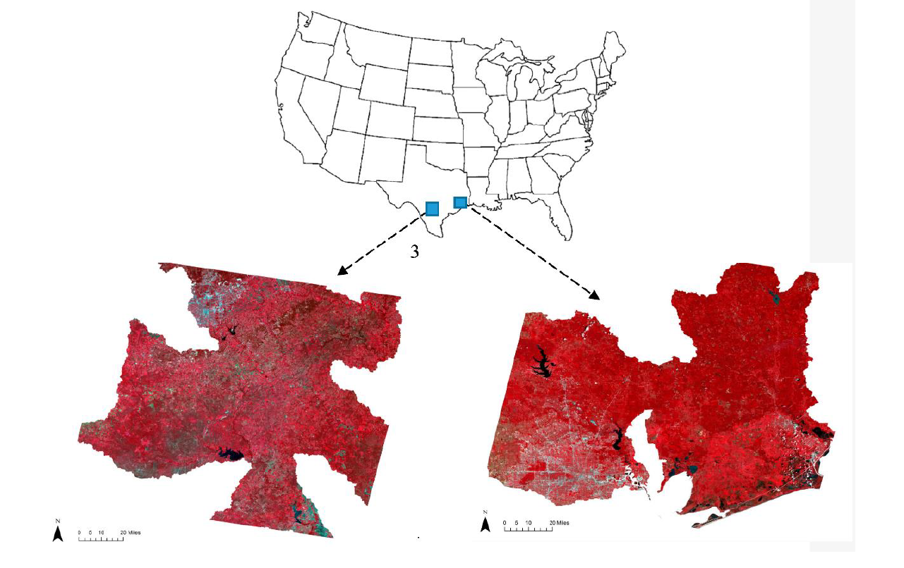
The two study sites are both located in the state of Texas, in south central U.S. (Figure 1). The South Texas site is situated between the Edwards Plateau to the northwest and the Gulf Coastal Plains to the southeast, and 200 km from the Gulf of Mexico. It is predominantly rural and consists of nine sub-basins, totaling an area of 23,625 km2 located in four major river basins: Nueces, San Antonio, Guadalupe, and San Antonio-Nueces. The climate is transitional humid subtropical, and the elevation is approximately 213 m above sea level. Vegetation is mostly oak and cedar woodland, grassland savanna, thorny brush, and riparian woodland. Most of the western half of the study area is part of the South Texas Plains, which stretch from the edges of the Hill Country into the subtropical regions of the Lower Rio Grande valley. The area is also prone to occasional severe weather from tornadoes and tropical cyclones and is prone to flooding. The average high temperature is 35 °C for both July and August, while the average low is 17 °C for December and January. The average annual precipitation for San Antonio is 836 mm. On average, the wettest months are May (119 mm) and June (109 mm) while the driest are January (41 mm) and February (43 mm).
The second study site is centered on the city of Houston in east Texas, and as such is actively irrigated and managed. The site has a total area of 22,000 km2 and consists of ten sub-basins located in four major river basins: San Jacinto, Trinity, Neches, and Neches-Trinity. The climate is humid subtropical, with mixed forested and temperate prairie grasslands. Generally, elevation rises around 25 cm per km, but coastal subsidence has caused the elevation to drop 3 m or more in some areas. Subsidence is caused by historical use of ground water and the extensive extraction of oil and natural gas. Lakes, rivers, and a large network of bayous and manmade canals make up the surface water. Occasional severe weather includes flooding, tornadoes, and tropical cyclones. The average high temperature in July and August is around 34 °C while in December and January it is 17 °C. The normal annual precipitation for Houston is 1150 mm. On average, the wettest months are May (113 mm) and July (132 mm), while the driest, February (81 mm) and March (61 mm).
2.1. Remotely Sensed Data
The data source for both sites is the Landsat 5 Thematic Mapper remote sensor, obtained from the USGS Global Visualization website (http://glovis.usgs.gov). The dates of the scenes for the South Texas site are 23 October 2009, 23 August 2010, and 11 September 2011. The dates for the Houston site are 22 August 2009, 25 August 2010, and 28 August 2011. Cloud-free anniversary dates were not available for either site; hence the next nearest dates were chosen. Archive maps from the US Drought Monitor (USDM) were used to verify drought conditions at the study sites. The USDM maps determined that there was a severe drought in southern Texas in 2009, but by 2010 there was little to no drought with higher than average rate of precipitation throughout the whole state. By 2011, exceptional drought conditions again persisted according to USDM for the vast majority of the state. Measurement of drought conditions is heavily dependent on land use/cover thematic categories, and as such an initial supervised classification was performed on the six remotely sensed scenes across both study sites using the maximum likelihood classifier. Training sites identified six land use/cover classes: urban, rocks/soil, forest, water, agriculture-1, and agriculture-2. The two classes of agriculture were identified as predominantly pasture and cropland respectively.
2.2. Remote Sensing Methodology
Remote sensing is routinely applied to the measurement of chlorophyll production, predominantly at the near infrared wavelengths. Droughts reduce chlorophyll production, which results in lower radiometric values at the near infrared. The established normalized difference vegetation index (NDVI) is widely used to quantify the photosynthetic capacity of vegetation. In addition, the bare soils index (BI) is also used to measure the density of vegetation as a comparison against completely bare soil, sparse canopies, and dense canopies. Finally, the normalized difference moisture index (NDMI) is a measure that is highly correlated with canopy water content [11,12]. To these indices, we add tasseled cap transformations (TCT) which facilitate direct comparisons across multiple scenes. TCT components which measure brightness, greenness, and wetness account for more than 97% of the spectral variability in a typical scene [13]. An advantage of TCT is that they are scene independent and accurate for monitoring land use/cover changes [14]. Lastly, we add change vector analysis (CVA); a measurement of the intensity (or magnitude) and direction between land use/cover variables in multidimensional space [13,15]. CVA determines small variations in class reflectance as a result of high intra-class differences caused by landscape heterogeneity [15,16]. By interpreting CVA intensity and the direction of change, the accumulated error that often occurs due to class-to-class comparisons between two image dates can be avoided. CVA also minimizes the need for collecting training and reference data for historical images, as unchanged locations can be used as reference data [13]. In the literature, a ‘from-to’ land use/class change analysis was used as a nested hierarchy of land use/cover to assess changes on the Pearl River Delta in China from increased economic activity [14]. Another study found that CVA was an effective method for monitoring changing ecosystems in wetland and riparian areas in southwest Montana, USA [13]. In addition, Landsat TM and ETM+ imagery was applied to map liana forests in the Bolivian Amazon by measuring changes in the spatial distribution of liana patches over a 14-year period from 1986 to 2000 [14]. Several other studies have shown the effectiveness of using CVA and TCT in unison for measuring forest disturbance as a result of events, such as deforestation, hurricanes, or tsunamis [15,16,17,18,19]. However, there is a dearth of studies that use a methodology that combines CVA and TCT for measuring land use/cover changes under severe, short-term drought events.
2.3. Change Vector Analysis
Change vector analysis (CVA) measures the magnitude and direction of change between dates across spectral space. Statistically, it is a variation of the Pythagorean Theorem that calculates the Euclidean distance of spectral change, defined as the position of a given pixel in Time 1 (T1) with Time 2 (T2), and the change that occurs between the two [20]. CVA eliminates the need to collect training or reference data for historical markers, as unchanged locations can be used as reference data [12]. It is flexible enough to be used with diverse sensor data, and radiometric change applications, including the monitoring of land use/cover change and ecosystem dynamics. For our sites, the raw index values were normalized to values between 0 and 1 in order to eliminate bias by any one index when calculating CVA magnitude. If two indicators are moderately correlated some land use/cover classes would be providing similar information but not for others. This makes them ideal for CVA as they provide four different change directions. Band statistics for NDVI and NDMI indicate there is also a moderate positive correlation, and hence it would be useful to explore their relationship, as this has not been done in other studies. The CVA method for magnitude was applied to NDVI and NDMI data using Equation (1),
where CM is change magnitude. CM values at or near zero identify areas with little or no change, while high CM values represent areas of high change. However, unchanged pixels fall within a range about the origin due to factors such as noise and imperfect normalization. This noise is removed by applying a threshold to CM; a threshold is determined by standard deviations [13,16,21,22]. The type of change is determined by examining change direction, calculated using NDVI and NDMI from Equation (2),
where atan2 converts rectangular coordinates to polar coordinates, and where α is the angle from the x-axis. This operation is based on sign and gives values that represent all quadrants in a Cartesian matrix. The output values are in the range of −π and π. Output from the arctangent function is in radians and converted to degrees by 180/π. 360 is added to all negative values to ensure output is within the range 0 to 360 degrees. The resulting angle in degrees is placed in one of four classes: +NDMI and +NDVI = chlorophyll increase, +NDMI and −NDVI = increase in wetness, −NDMI and −NDVI = bare soil expansion, and −NDMI and +NDVI = decrease in wetness.
Using tasseled cap bands of brightness, greenness and wetness (BGW), magnitude and direction of change is determined by differences between each band and between each date. Brightness is usually associated with bare soil or bare ground, with an increasing brightness indicating a change towards bare soil while a decreasing brightness indicates a change away. However, if for example lianas are considerably brighter spectrally than dense forest vegetation, then increasing brightness may be an indication of the increasing abundance of lianas in vegetation [17]. Moreover, as brightness is a weighted sum of all six reflective bands of Landsat, it can be interpreted as the overall brightness or albedo at the surface. Greenness is directly related to chlorophyll presence and photosynthetic activity, and hence changes in greenness are related to increase or decrease in vegetation [13,14,17,23,24,25,26,27,28]. Wetness can be an indicator of vegetation density, soil moisture, and hence decrease in wetness indicates declining vegetation health or senescence [11,14]. However, the presence of water, as in flooded forests, also adds wetness and hence increase in wetness may be related to actual increase of water. Although TCT was initially used for agricultural applications, it is also useful for assessing structural characteristics of forest environments. An advantage of TCT over other statistical methods, such as principal components analysis is that TCT is independent of the individual scenes while PCA is scene dependent [29]. Hence, changes in TCT components over time can be related to changes in vegetation attributes. The CVA method for magnitude was applied to tasseled cap components using Equation (3),
where axes x, y and z correspond to tasseled cap brightness (B), greenness (G), and wetness (W) respectively.
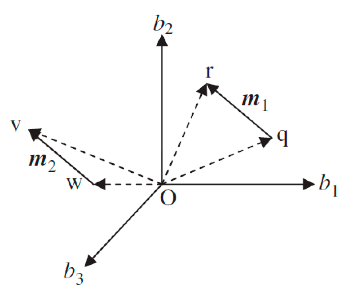
Using three TCT (BGW), the change vector is represented in three-dimensional space where b1, b2, and b3 are the three spectral bands and m1 and m2 are example change vectors (Figure 2). The direction of the change occurring among the three components is calculated by Equation (4).
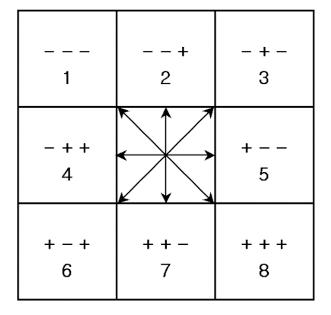
Change direction is measured as the angle of the change vector from the pixel value at Time 1 to the corresponding pixel value at Time 2. Again, using three bands of TCT (BGW), the resulting change classes will number 23 or eight (Figure 3).
3. Results and Discussion
Results from CVA were assessed for accuracy using 200 random sample points. Post-classification comparison (PCC) maps were created and used as reference to produce a ‘change/no change’ error matrix based on the random points. Supported by visual interpretation of the remotely sensed imagery from Google Earth, overall accuracy and Kappa coefficients for both the Houston and South Texas sites were found to be higher for the NDVI-NDMI and TCT calculations when compared with NDVI-BI.
The supervised classification highlights the severity of the drought year in 2011 (Table 1). For both sites, forest land cover decreases markedly between 2010 and 2011; a moderate fall from 58.8% to 47.9% in Houston, and an almost halving from 15.0% to 8.6% in South Texas. Agriculture too declines between 2010, but only for the more rural site of South Texas, not for the more urbanized Houston site. It’s worth noting that both forest and agriculture increase between the relatively moderate drought year of 2009 to the wet-to-average year of 2010, but only slightly; a matter of a few percentage points. In contrast, urban and rock/soil (which are highly co-dependent spectrally) increase in the 2011 severe drought year. Water bodies remain the same across all three years.
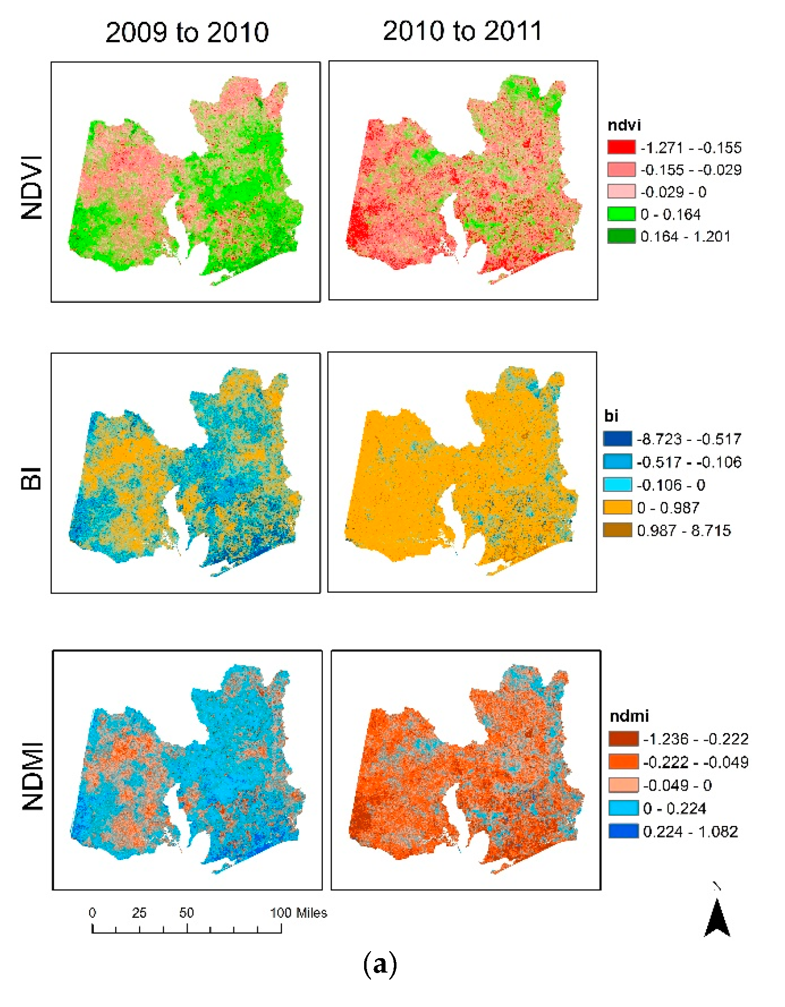
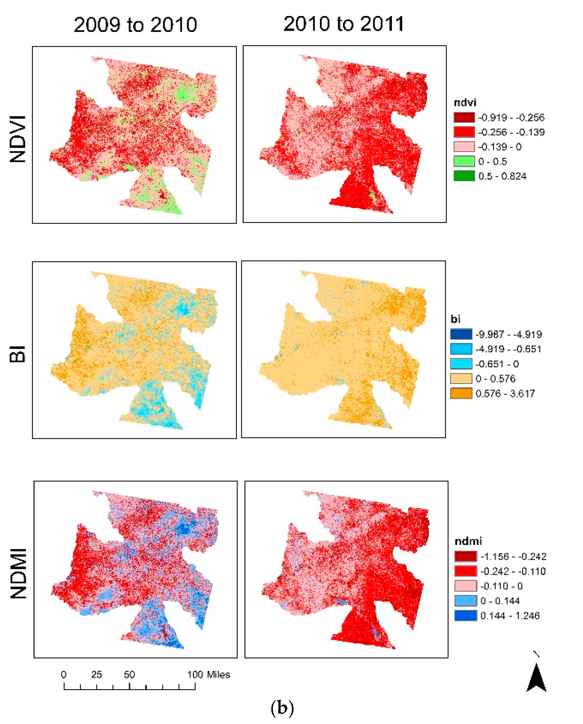
To spatially visualize these changes in land use/cover we can use image difference maps based on NDVI, BI, and NDMI. (Figure 4a,b). Across the majority of the area of the Houston site, image differences between the two years (i.e., 2009 and 2010) when conditions were getting wetter are substantiated by increasing NDVI values, decreasing BI values, and increasing NDMI values. All three indices reverse for the 2010 to 2011 image differences, which confirms drying conditions. For the South Texas site, the 2009 to 2010 difference illustrates that a majority of the area is shifting towards less green and brighter conditions respectively (according to NDVI and BI), although NDMI values indicate that approximately half of the area is moving towards improved wet conditions. This is an indication, to some degree, of a persisting drought. It maybe be explained by the use of an image for 2009 that was captured in October—a relatively wet month for the San Antonio region, while the 2010 image was taken during the month of August—which is typically one of the driest months. However, the severe drought of 2011 is again highlighted by expected decreasing NDVI values, increasing BI values, and decreasing NDMI values; just like the Houston site.
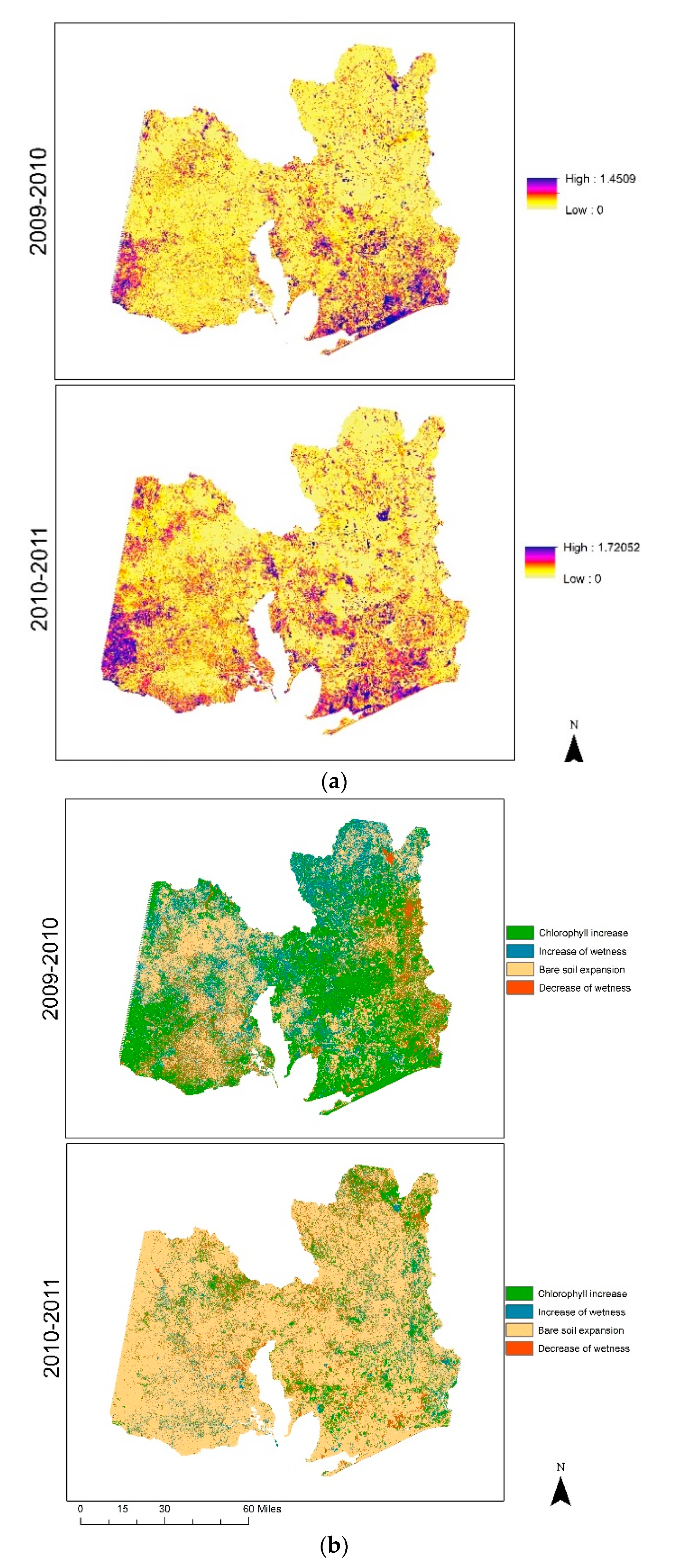
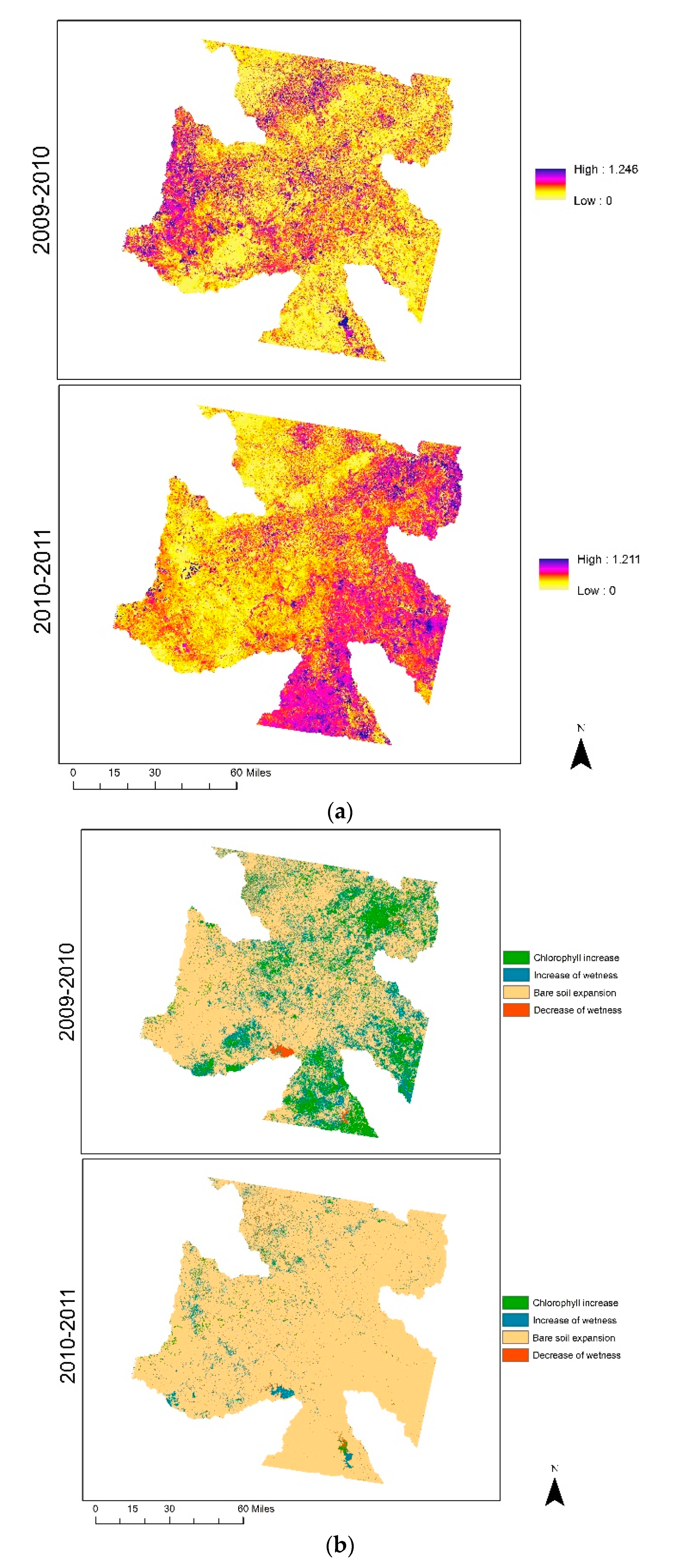
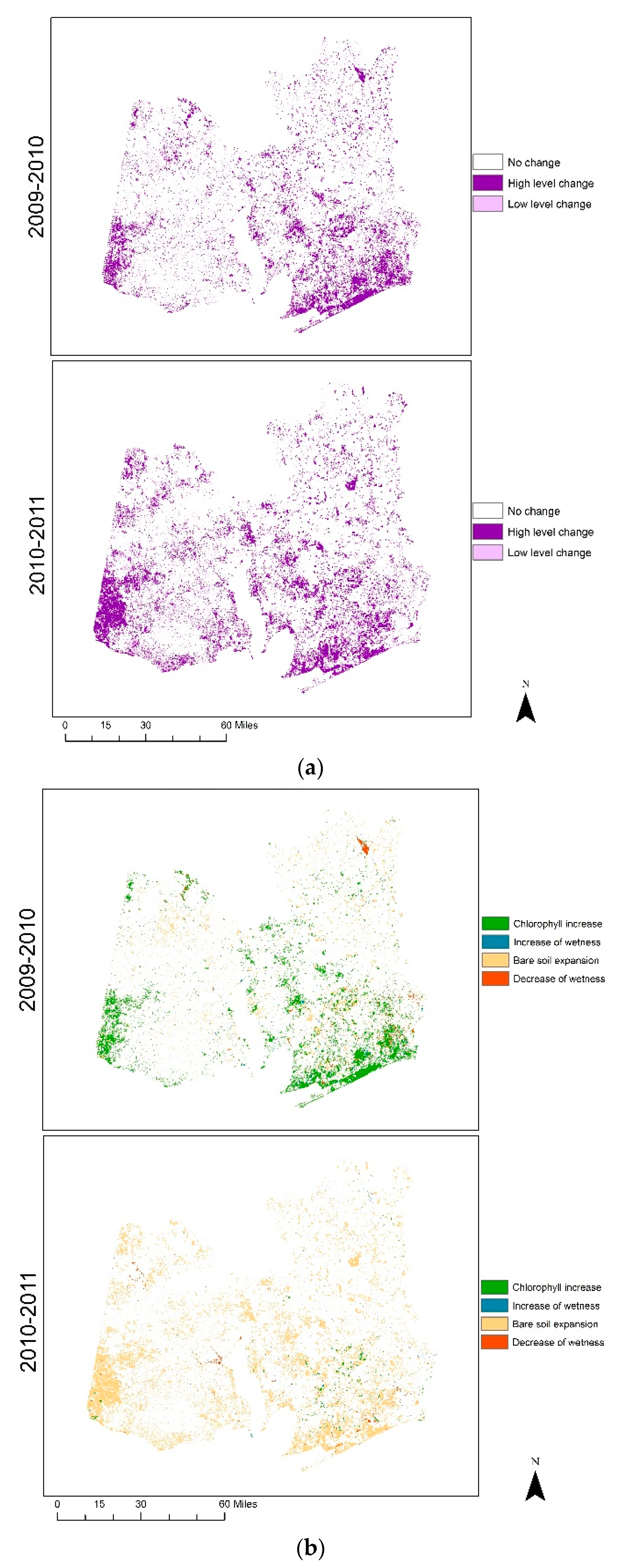
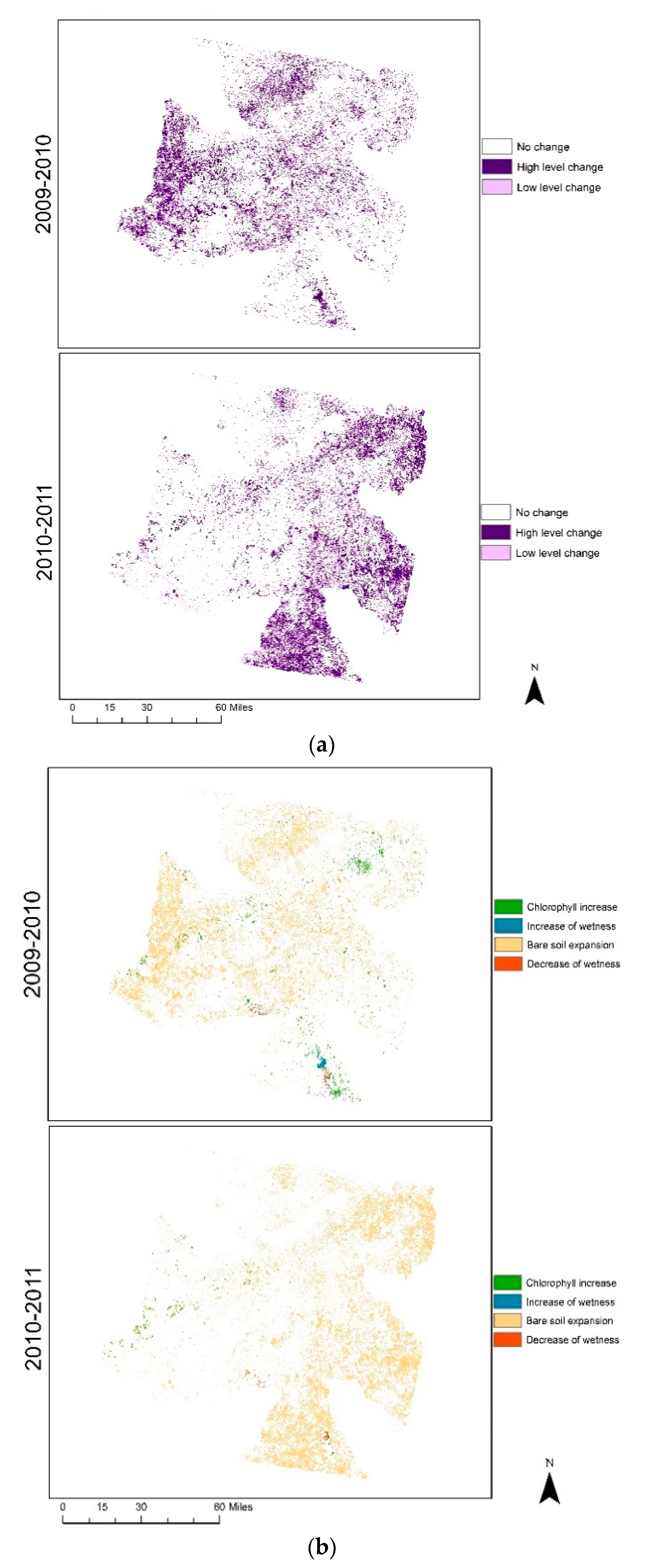
We can use CVA to further illustrate changing wetness and drying. Using NDVI and NDMI as the basis for measuring magnitude and change direction, the period 2009 to 2010 experienced chlorophyll expansion, and an increase in wetness over most of the Houston site (Figure 5a). By contrast, between 2010 and 2011 most areas experienced bare soil expansion (Figure 5b). Similar results were evident for South Texas (Figure 6a,b). Applying a threshold identifies which pixels represent change and which represent no change. We used 0.5 standard deviation threshold as the low change cutoff and 1.0 standard deviation for the high change cutoff (in line with work by [8,10,16,18,28,30]). Using high change pixels (dark purple in Figure 7a and Figure 8a) the spatial contrast in wetter and drier year is clearly demonstrated. For example, for Houston, those dark purple pixels mostly correspond to chlorophyll increase (green), indicating wetter conditions for years 2009 to 2010, while for the years 2010 to 2011 they mostly correspond to bare soil expansion (yellow), representing the severe drought (Figure 7b). However, the same situation is clearly not evident for South Texas (Figure 8b). The high level change pixels for the years 2009 to 2010 to not correspond to widespread chlorophyll increase (only a few, especially in the south of the site) but instead equate to bare soil expansion. More evidence that agriculture did not recover as quickly in South Texas as it did in Houston. The situation for the years 2010 to 2011 again, like Houston, illustrate the severity of the drought with predominance of bare soil expansion.
Most pixels are unchanged, both for 2009 to 2010 (almost 82% for Houston and over 78% for South Texas) and for 2010 to 2011 (over 78% for Houston and over 73% for South Texas) (Table 2). Over the remaining, more pixels represented high level changes; of those slightly more were for the 2010 to 2011 years, indicating a more rapid change to drought conditions than the wetting period of the previous year. When examining individual land use/cover classes, the majority of high level changes on the Houston site were pixels representing agriculture or forest; precisely the ones most likely to be affected by chlorophyll increase or bare soil expansion in times of precipitation or sustained aridity. For South Texas, agriculture changed the most within the high threshold as chlorophyll increase accounted for around 60% of the total landscape. However, in the years 2010 to 2011, agriculture accounted for 90% of high-level change, this time as a result of bare soil expansion.
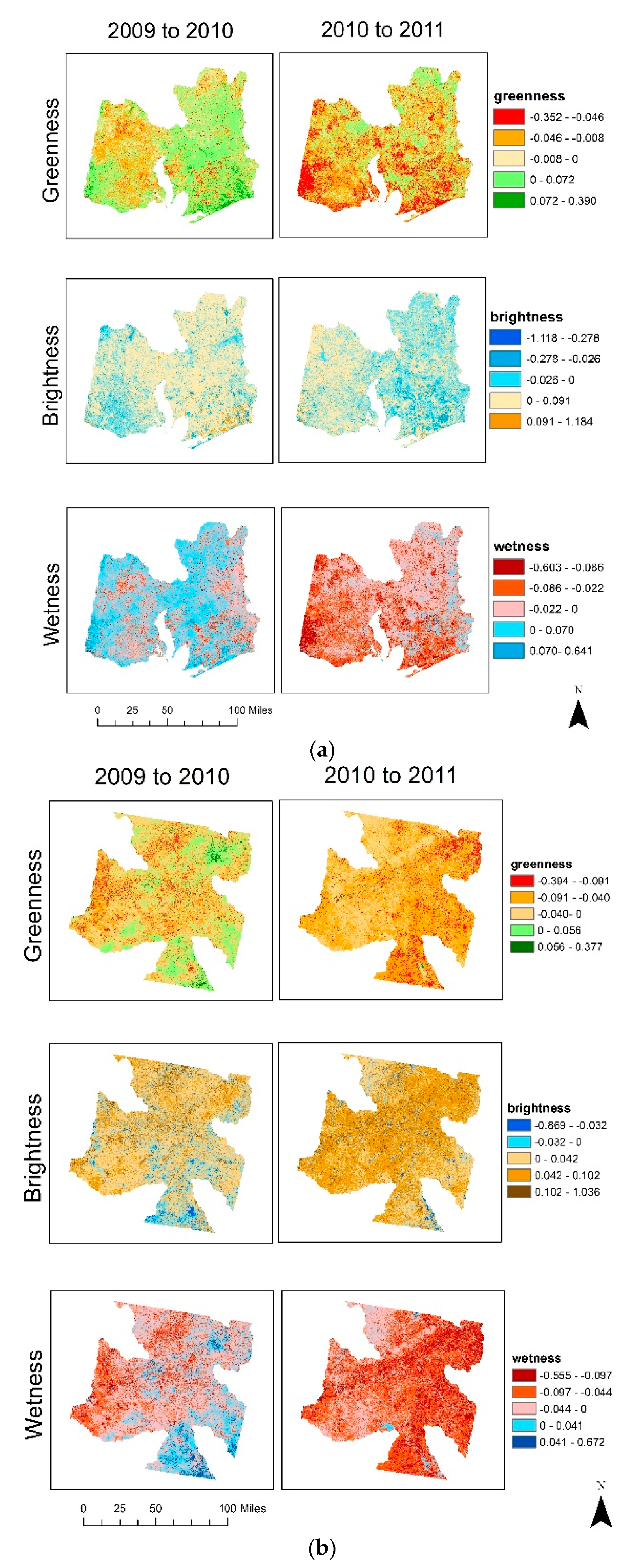
Image differences using TCT brightness, greenness, and wetness are consistent with the semi-drought conditions present in 2009, improving to average wet conditions in 2010, and then the exceptionally dry year of 2011 for Houston (Figure 9a). Brightness however, is somewhat of an outlier as for 2009–2010, large areas of the scene appear to be increasing in brightness while in 2010–2011, areas are decreasing in brightness. In comparison many parts of the South Texas site indicate drying conditions for 2009–2010 period (again, because the 2010 image was taken in August), and then deteriorating conditions towards drought in 2011 (Figure 9b).
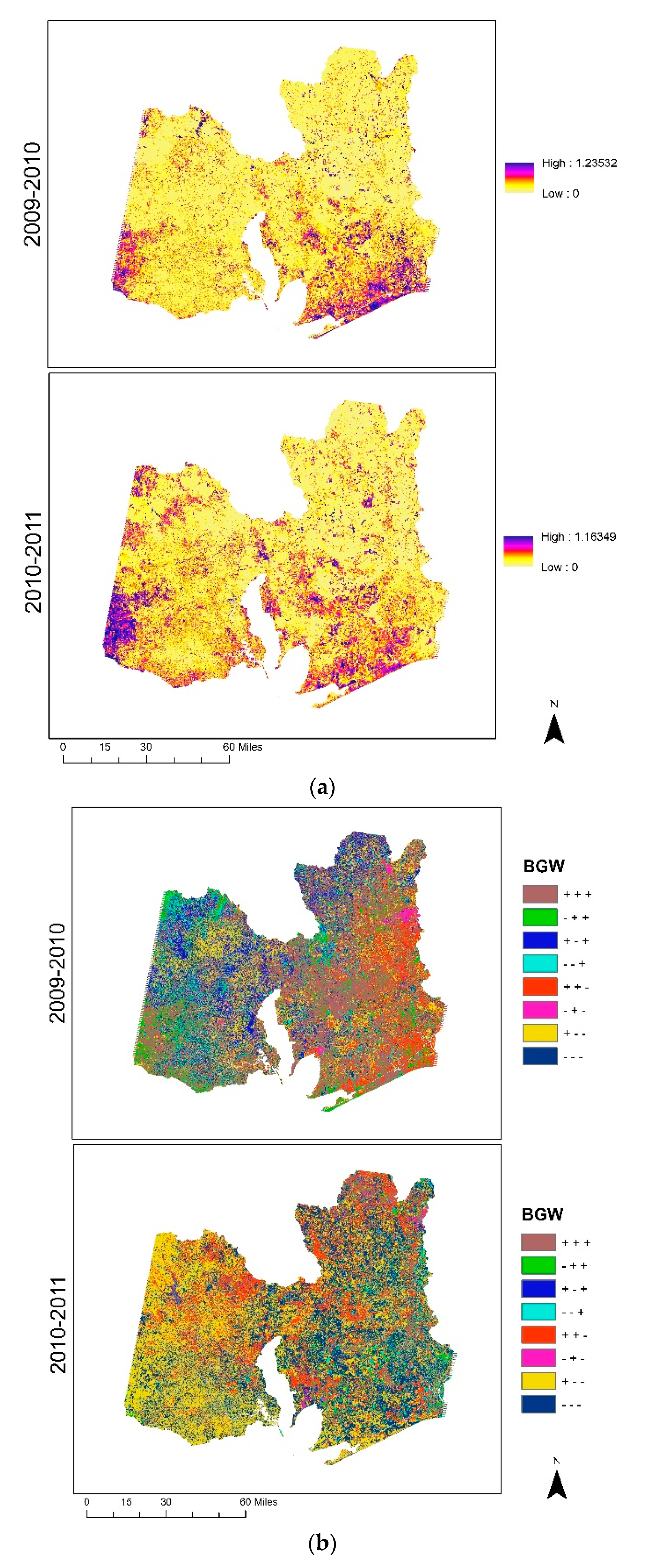
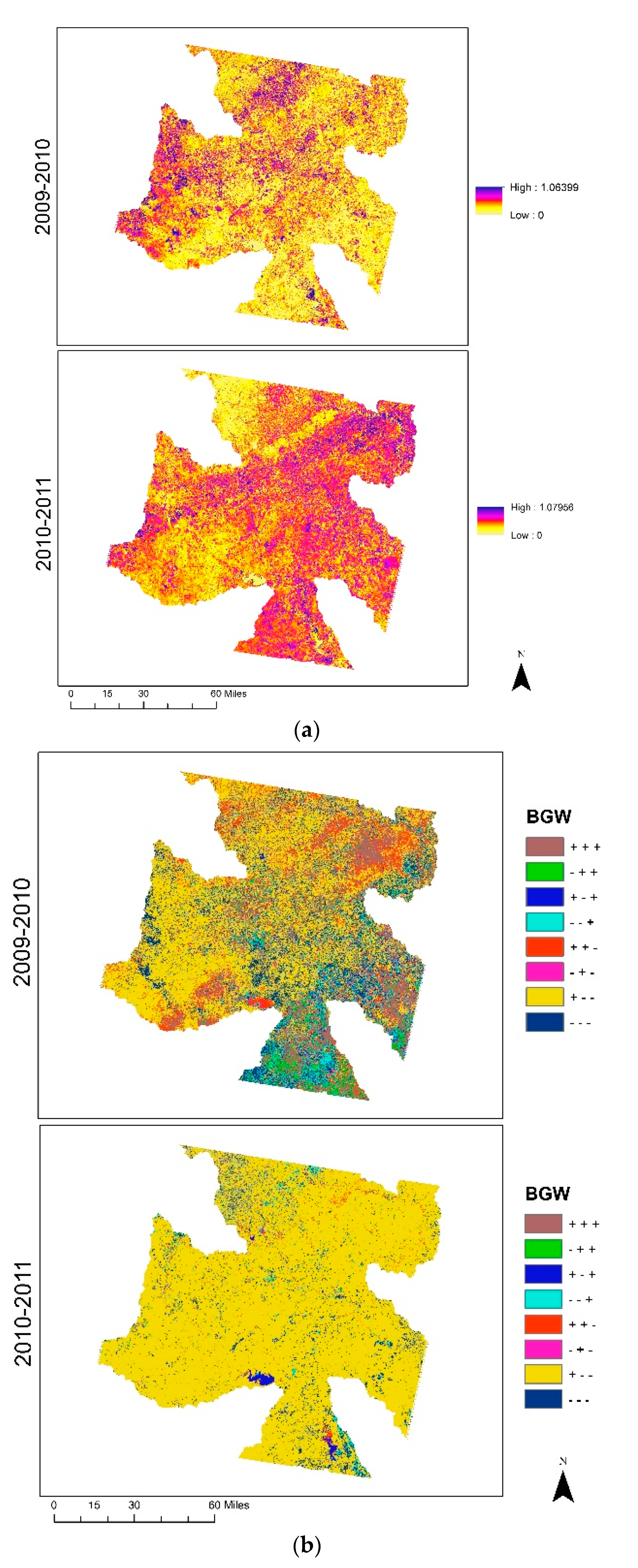
The two study sites demonstrate variations in change vector magnitude. The Houston site experienced low-level changes across the majority of its area-other than patches in the south and south-west (Figure 10a). However, at the South Texas site higher-level changes are apparent throughout the whole area, especially for the 2010 to 2011 years (Figure 11a). In terms of change direction using TCT, it is difficult to discern which change class dominates the 2009 to 2010 years across Houston (Figure 10b). However, for the 2010 to 2011 years there is a noticeable dominance of the yellow class, particularly on the west side; this class corresponds with increases in brightness (B), combined with a decrease in both greenness (G) and wetness (W). Similar results are evident for the South Texas site where many areas to the west and center appear to be dominated by, again, the yellow class for the 2009 to 2010 years, and almost the entire scene for the 2010 to 2011 years. Both indicate a move towards increased drying (Figure 11b). The two threshold cutoffs of 0.5 standard deviation to determine pixels of low-level change, and 1.0 standard deviation to represent pixels of high-level change resulted in 85% and 82% of the sites with no change pixels for the 2009 to 2010 and 2010 to 2011 years respectively. High-level change is higher for the 2010 2011 years at just under 12% compared with around 9.5% for the 2009 2010 years. This indicates that a greater amount of change as well as a greater intensity of change occurred in the 2010 to 2011 years.
In terms of change direction masked by the high threshold cells, it is difficult to discern the proportions of the overall change types. However, individually, for the Houston site, the higher change classes are, in descending order for 2009 the 2010 years: B+ G+ W+, B+ G− W−, B− G+ W+, and B+ G+ W−. For the 2010 to 2011 years, the only substantial change classes are B+ G− W− at over 60% of the high threshold and B− G− W− at around 25%. It is interesting to note the presence of certain change classes when the expected change is known. For example, B− G+ W+ is expected during a change towards normal, wet conditions; however, the presence of B+ G− W− indicate that for significant areas there was continuing drought in 2010 from the previous year. As for B+ G+ W−, certain vegetation types may have higher brightness values than their background, suggesting that in some cases an increase in vegetation may result in an increase in brightness. For the South Texas site, B+ G− W− covered over 60% of the high threshold for the 2009 to 2010 years while it is approximately 90% for the 2010 to 2011 years.
In terms of actual acreage change, agricultural land use contributed around 42% of the total changed cells for the 2009 to 2010 years at the Houston site, and over 50% for the 2010 to 2011 years. In contrast, agricultural land use at the South Texas site contributed up to 76% of the changed cells for the 2009 to 2010 years, and as high as 86% for the 2010 to 2011. Similarly, forest land cover changes are much higher for the South Texas site: 30% and 7% for the 2009 to 2010 and the 2010 to 2011 years respectively, compared to 21% and 1% across the same years for the Houston site (Table 3). Both support the notion of the droughts affecting the more rural South Texas site.
Changes between land use/cover types is even more pronounced during drought conditions. Using the high-level threshold cut-off from the TCT we can measure the most prevalent changes; we call them the top three “from-to” land use/cover types (Table 4). While it may be difficult to discern the precise type, eight change directions emerge from our results. For example, the move away from drought (the 2009 to 2010 years) is illustrated by the directions B+ G+ W+ and B− G+ W+, which represent changes towards green vegetation-mostly increases in agriculture and forest. Again, this is more apparent for the Houston site where proximity to an urban area would mean higher levels of irrigation (Figure 4a). In contrast, the more rural South Texas site is indicative of B+ G− W−, which represents a decrease in vegetation and a trend towards drying conditions. The level is above 90% for the severe drought event years of 2010 to 2011, compared to 65% for the Huston site for the same period. Incidentally, B+ G− W+ and B− G− W+ represent changes towards urbanization, which ideally should be masked out for an analysis of changes caused by drought. It is also interesting to see that B− G+ W− mostly affects urban classes. For the remaining change directions however, the type of change that occurs is less clear.
4. Conclusions
Using post-classification correction (PCC) based on ancillary data and knowledge-based logic rules, the overall accuracies for NDVI-NDMI and TCT across both sets of years for the Houston site are consistently between 81% and 84%, with Kappa coefficients varying a little more, between 45% and 52%. For the South Texas site, overall accuracies are much lower, ranging between 58% and 65%, with the Kappa coefficients, also lower, between 43% and 51%. However, these accuracies are higher than the NDVI-BI calculation, which has an overall accuracy and Kappa coefficient for the first and second year pairs of 73% and 21%, and 71% and 22% respectively. Overall accuracy and Kappa coefficient for the South Texas site for the first and second year pairs of NDVI-NDMI is 73% and 43%, and 73% and 46%, respectively. For the 2009 to 2010 years, the TCT overall accuracy is 75% with a kappa coefficient of 47% while the 2010 to 2011 years has an overall accuracy of 76% and a Kappa coefficient of 51%. For the South Texas site, the accuracies based on PCC are also higher than the NDVI-BI calculation, which indicated an overall accuracy and Kappa coefficient for the first and second year pairs of 65% and 21%, and 61% and 24% respectively. Generally speaking, the PCC results were more likely to identify changed cells within the sampled points, indicating a greater sensitivity towards change. We are calculating lower producer’s accuracy for changed cells indicating that the CVA results were not as sensitive to change as the PCC. This may have been because the selected threshold was too high, thus excluding certain land use/cover changes from the analysis. The high overall accuracy and good kappa coefficients indicate the CVA was effective in detecting vegetation dynamics caused by drought. These are the summaries. For full accuracy assessment, contact the authors. Our results are also in line with the publicly available National Land Cover Databases (NLCD) (mrlc.gov). The U.S. Geological Survey (USGS) who produce NLCD updates also use Landsat sensor imagery but their methodology is based on multi-sourced training data and decision-tree land cover classifications. Given, their wide definitions of land cover, they report accuracies for the conterminous U.S. between 71% and 97% [32].
Remote sensing is crucial for environmental monitoring. Data on land use/cover at various scales and for various dates contribute to models of environmental change, and in return, fuel many local and federal environmental policies. Sudden sort-term drought events decimate ecosystems and threaten agricultural livelihood. By developing a methodology based on remote sensing data, we are contributing to research on how to measure more precisely the dryness of land use/cover using established image analysis statistics. Our methodology measures sudden dryness using change vector analysis of NDVI-NDMI, and the brightness, greenness, and wetness variables from tasseled cap. Together these statistics measure land use/cover changes during severe sudden short-term drought events by calculating not only vegetation and bare soil indices, but also determine the intensity of change (magnitude) and the type of change (direction). Although these image-processing techniques have long been available, they have as yet been applied to assessing drought conditions in land use/cover changes. One reason may be that sudden dryness is not considered serious enough for multiple studies. Another reason may be that these techniques are underrated. With increasing fluctuations in weather linked primarily to climate change, research on precise measurements of sudden aridity and prolonged drought are gaining prominence for assessing ecosystem disturbances, agricultural loss, and even threat to life, especially if dryness leads to more fires. As well, in terms of underrated techniques, the NDVI-NDMI combination continues to produce reliable and important measures of vegetation and moisture. So too tasseled cap transforms that measure bare soil and vegetation. In terms of change vector, we have included an improvement using the arctangent function based on two arguments, ATAN2 which produces results in all four possible quadrants and complete characterization of all possible change directions.
Our test sites are from satellite sensor images taken of notoriously high frequency sudden short-term drought events over the southern state of Texas. A ‘from-to’ land use/cover change assessment was made for each direction class to discern any patterns with any particular change directions as a result of severe aridity. Overall accuracies and Kappa coefficients for both the Houston and South Texas sites were found to be higher for the NDVI-NDMI and TCT calculations when compared with the NDVI-BI results. CVA was performed on NDVI and NDMI with change direction classes as expected when predicting drought. However, the relationships between TCT brightness, greenness and wetness and their ability to detect change was more difficult to determine by their type of change in each of the directions, and hence they may be context dependent. In terms of short-term droughts in humid subtropical climatic regions, such as the south and southeast United States, some interesting change directions were evident. For example, for both sites the directions B+ G+ W+ and B− G+ W+ change land use/cover classes towards green vegetation, predominantly agriculture and forest. Meanwhile B+ G− W− appears to move towards drying and a decrease of vegetation or towards rocks and soil land cover classes. The presence of B+ G− W− indicates that for significant areas there was continuing drought in 2010 from the previous year. Also, it appears that B+ G− W+ and B− G− W+ capture changes towards urbanization, which ideally should be masked out for an analysis of changes caused by drought. Meanwhile the change direction B− G+ W− appears to only affect urban land use. For other change directions however, the type of change is less clear.
The outcome of our work demonstrates that the relationship between NDVI and NDMI, and between TCT variables applied to CVA calculations are effective in measuring land use/cover changes as a result of high annual precipitation variability. Moreover, CVA measures which land use/cover classes experienced the most changes, in addition to the type of change and direction of change. Further studies should test and compare our results with other land use/cover change detection methods, such as image ratioing and principal components analysis.
Author Contributions
Conceptualization, methodology, software, validation, formal analysis, and writing—original draft preparation S.R.; writing—review and editing, and supervision, V.M.
Funding
This research was partly funded by Florida State University, Library Resources.
Conflicts of Interest
The authors declare no conflict of interest.
References
- Combs, S. The Impact of the 2011 Drought and Beyond; Texas Comptroller of Public Accounts: Austin, TX, USA, 2012. [Google Scholar]
- Mishra, A.K.; Singh, V.P. Drought modeling—A review. J. Hydrol. 2011, 403, 157–175. [Google Scholar] [CrossRef]
- Mu, Q.; Zhao, M.; Kimball, J.S.; McDowell, N.G.; Running, S.W. A remotely sensed global terrestrial drought severity index. Bull. Am. Meteorol. Soc. 2013, 94, 83–98. [Google Scholar] [CrossRef]
- AghaKouchak, A.; Farahmand, A.; Melton, F.S.; Texeira, J.; Anderson, M.C.; Wardlow, B.D.; Hain, C.R. Remote sensing of drought: Progress, challenges and opportunities. Rev. Geophys. 2015, 53, 452–480. [Google Scholar] [CrossRef] [Green Version]
- Ahmadi, B.; Ahmadalipour, A.; Tootle, G.; Moradkhani, H. Remote sensing of water use efficiency and terrestrial drought recovery across the contiguous United States. Remote Sens. 2019, 11, 731. [Google Scholar] [CrossRef]
- Schwalm, C.R.; Anderegg, W.R.L.; Michalak, A.M.; Fisher, J.B.; Biondi, F.; Koch, G.; Litvak, M.; Ogle, K.; Shaw, J.D.; Wolf, A.; et al. Global patterns of drought recovery. Nature 2017, 548, 202–205. [Google Scholar] [CrossRef] [PubMed]
- Yu, Z.; Wang, J.; Liu, S.; Rentch, J.S.; Sun, P.; Lu, C. Global gross primary productivity and water use efficiency changes under drought stress. Environ. Res. Lett. 2017, 12, 014016. [Google Scholar] [CrossRef] [Green Version]
- Warner, T. Hyperspherical direction cosine change vector analysis. Int. J. Remote Sens. 2005, 26, 1201–1215. [Google Scholar] [CrossRef]
- Siwe, R.N.; Koch, B. Change vector analysis to categorise land cover change processes using the tasseled cap as biophysical indicator. Environ. Monit. Assess. 2008, 145, 227–235. [Google Scholar] [CrossRef]
- Carvalho, O.A., Jr.; Guimares, R.F.; Gillespie, A.R.; Silva, N.C.; Gomes, R.A.T. A new approach to change vector analysis using distance and similarity measures. Remote Sens. 2011, 3, 2473–2493. [Google Scholar] [CrossRef]
- Jin, S.; Sader, S.A. Comparison of time series tasseled cap wetness and the normalized difference moisture index in detecting forest disturbances. Remote Sens. Environ. 2005, 94, 364–372. [Google Scholar] [CrossRef]
- Vorovencii, I. A change vector analysis technique for monitoring land cover changes in Copsa Mica, Romania, in the period 1985–2011. Environ. Monit. Assess. 2014, 186, 5951–5968. [Google Scholar] [CrossRef]
- Baker, C.; Lawrence, R.L.; Montagne, C.; Patten, D. Change detection of wetland ecosystems using Landsat imagery and change vector analysis. Wetlands 2007, 27, 610–619. [Google Scholar] [CrossRef]
- Seto, K.C.; Woodcock, C.E.; Song, C.; Huang, X.; Lu, J.; Kaufmann, R.K. Monitoring land-use change in the Pearl River Delta using Landsat TM. Int. J. Remote Sens. 2002, 23, 1985–2004. [Google Scholar] [CrossRef]
- Landmann, T.; Schramm, M.; Huettich, C.; Dech, S. MODIS-based change vector analysis for assessing wetland dynamics in Southern Africa. Remote Sens. Lett. 2013, 4, 104–113. [Google Scholar] [CrossRef]
- Chen, J.; Gong, P.; He, C.; Pu, R.; Shi, P. Land-use/land-cover change detection using improved change-vector analysis. Photogram. Engin. Remote Sens. 2003, 69, 369–379. [Google Scholar] [CrossRef]
- Foster, J.R.; Townsend, P.A.; Zganjar, C.E. Spatial and temporal patterns of gap dominance by low-canopy lianas detected using EO-1 Hyperion and Landsat Thematic Mapper. Remote Sens. Environ. 2008, 112, 2104–2117. [Google Scholar] [CrossRef]
- Healey, S.P.; Cohen, W.B.; Zhiqiang, Y.; Krankina, O.N. Comparison of Tasseled Cap-based Landsat data structures for use in forest disturbance detection. Remote Sens. Environ. 2005, 97, 301–310. [Google Scholar] [CrossRef]
- Nackaerts, K.; Vaesen, K.; Muys, B.; Coppin, P. Comparative performance of a modified change vector analysis in forest change detection. Int. J. Remote Sens. 2005, 26, 839–852. [Google Scholar] [CrossRef]
- Flores, S.E.; Yool, S.R. Sensitivity of change vector analysis to land cover change in an arid ecosystem. Int. J. Remote Sens. 2007, 28, 1069–1088. [Google Scholar] [CrossRef]
- Johnson, R.D.; Kasischke, E.S. Change vector analysis: A technique for the multispectral monitoring of land cover and condition. Int. J. Remote Sens. 1998, 19, 411–426. [Google Scholar] [CrossRef]
- Karnieli, A.; Qin, Z.; Wu, B.; Panov, N.; Yan, F. Spatio-temporal dynamics of land-use and land-cover in the Mu Us Sandy Land, China, using the change vector analysis technique. Remote Sens. 2014, 6, 9316–9339. [Google Scholar] [CrossRef]
- Kennedy, R.E.; Cohen, W.B.; Schroeder, T.A. Trajectory-based change detection for automated characterization of forest disturbance dynamics. Remote Sens. Environ. 2007, 110, 370–386. [Google Scholar] [CrossRef]
- Roemer, H.; Kaiser, G.; Sterr, H.; Ludwig, R. Using remote sensing to assess tsunami-induced impacts on coastal forest ecosystems at the Andaman Sea coast of Thailand. Nat. Hazards Earth Sys. Sci. 2010, 10, 729–745. [Google Scholar] [CrossRef]
- Wang, F.; Xu, Y.J. Comparison of remote sensing change detection techniques for assessing hurricane damage to forests. Environ. Monit. Assess. 2010, 162, 311–326. [Google Scholar] [CrossRef]
- Lorena, R.B.; Santos, J.R.; Shimabukuro, Y.E.; Brown, I.F.; Kux, H.J.H. A change vector analysis technique to monitor land use/land cover in SW Brazilian amazon: Acre State. ISPRS Arch. 2002, 34, 8. [Google Scholar]
- Shine, T.; Mesev, V. Remote sensing and GIS for ephemeral wetland monitoring and sustainability in southern Mauritania. In Integration of GIS and Remote Sensing; Mesev, V., Ed.; Wiley & Sons: Chichester, UK, 2007; pp. 269–290. [Google Scholar]
- Baisantry, M.; Negi, D.S.; Manocha, O.P. Change vector analysis using enhanced PCA and inverse triangular function-based thresholding. Def. Sci. J. 2012, 62, 236–242. [Google Scholar] [CrossRef]
- Han, T.; Wulder, M.A.; White, J.C.; Coops, N.C.; Alvarez, M.F.; Butson, C. An efficient protocol to process Landsat images for change detection with tasseled cap transformation. IEEE Geosci. Remote Sens. Lett. 2007, 4, 147–151. [Google Scholar] [CrossRef]
- Varshney, A.; Arora, M.K.; Ghosh, J.K. Median change vector analysis algorithm for land-use land-cover change detection from remote-sensing data. Remote Sens. Lett. 2012, 3, 605–614. [Google Scholar] [CrossRef]
- Yoon, G.-W.; Yun, Y.B.; Park, J.-H. Change vector analysis: Detecting of areas associated with flood using Landsat TM. In Proceedings of the IEEE International Geoscience & Remote Sensing Symposium, Tolouse, France, 21–25 July 2003; pp. 3386–3388. [Google Scholar]
- Yang, L.; Jin, S.; Danielson, P.; Homer, C.; Gass, L.; Bender, L.; Case, A.; Costello, C.; Dewitz, J.; Fry, J.; et al. A new generation of the United States National Land Cover Database: Requirements, research priorities, design, and implementation strategies. ISPRS J. Photogram. Remote Sens. 2018, 146, 108–123. [Google Scholar] [CrossRef]
Figure 1.
Study Sites: (left) South Texas, (right) Houston.

Figure 2.
Representation of possible change vectors in three dimensions (after [30]).
Figure 2.
Representation of possible change vectors in three dimensions (after [30]).

Figure 3.
Possible change sector codes in three bands (after [31]).
Figure 3.
Possible change sector codes in three bands (after [31]).

Figure 4.
Image differences for 2009 and 2010, and 2010 and 2011 using NDVI, BI, and NDMI for (a) Houston, (b) South Texas.
Figure 4.
Image differences for 2009 and 2010, and 2010 and 2011 using NDVI, BI, and NDMI for (a) Houston, (b) South Texas.


Figure 5.
(a) Change vector magnitude for NDVI and NDMI for Houston site; (b) change vector direction for NDVI and NDMI for Houston site.
Figure 5.
(a) Change vector magnitude for NDVI and NDMI for Houston site; (b) change vector direction for NDVI and NDMI for Houston site.

Figure 6.
(a) Change vector magnitude for NDVI and NDMI for South Texas site. (b) Change vector direction for NDVI and NDMI for South Texas site.
Figure 6.
(a) Change vector magnitude for NDVI and NDMI for South Texas site. (b) Change vector direction for NDVI and NDMI for South Texas site.

Figure 7.
(a) Change vector magnitude with threshold for NDVI and NDMI for Houston site. (b) Change vector direction with threshold for NDVI and NDMI for Houston site.
Figure 7.
(a) Change vector magnitude with threshold for NDVI and NDMI for Houston site. (b) Change vector direction with threshold for NDVI and NDMI for Houston site.

Figure 8.
(a) Change vector magnitude with threshold for NDVI and NDMI for South Texas site. (b) Change vector direction with threshold for NDVI and NDMI for South Texas site.
Figure 8.
(a) Change vector magnitude with threshold for NDVI and NDMI for South Texas site. (b) Change vector direction with threshold for NDVI and NDMI for South Texas site.

Figure 9.
Image differences for 2009 and 2010, and 2010 and 2011 using TCT brightness, greenness, and wetness NDVI, BI, and NDMI for (a) Houston, (b) South Texas.
Figure 9.
Image differences for 2009 and 2010, and 2010 and 2011 using TCT brightness, greenness, and wetness NDVI, BI, and NDMI for (a) Houston, (b) South Texas.

Figure 10.
(a) Change vector magnitude for TCT BGW at Houston site. (b) Change vector direction for TCT BGW at Houston site.
Figure 10.
(a) Change vector magnitude for TCT BGW at Houston site. (b) Change vector direction for TCT BGW at Houston site.

Figure 11.
(a) Change vector magnitude for TCT BGW at South Texas site. (b) Change vector direction for TCT BGW at South Texas site.
Figure 11.
(a) Change vector magnitude for TCT BGW at South Texas site. (b) Change vector direction for TCT BGW at South Texas site.


Table 1.
Land use/cover changes (%) from supervised classification: Houston (H), South Texas (ST).
| Land Use/Cover | 2009 (H) | 2009 (ST) | 2010 (H) | 2010 (ST) | 2011 (H) | 2011 (ST) |
|---|---|---|---|---|---|---|
| Urban | 10.6 | 10.5 | 11.3 | 5.2 | 11.4 | 18.4 |
| Rocks/Soil | 7.2 | 4.0 | 5.2 | 7.5 | 14.1 | 28.4 |
| Agriculture | 23.8 | 71.0 | 23.5 | 71.6 | 25.4 | 44.0 |
| Forest | 57.0 | 14.0 | 58.8 | 15.0 | 47.9 | 8.6 |
| Water | 1.3 | 0.6 | 1.3 | 0.7 | 1.3 | 0.6 |
Table 2.
Changes for Houston and South Texas sites.
| NDVI-NDMI (2009–2010) | Houston Area (%) | Houston Area (km2) | S Texas Area (%) | S Texas Area (km2) |
|---|---|---|---|---|
| No change | 81.9 | 18,049 | 75.5 | 17,829 |
| Low level change | 6.2 | 1372 | 9.6 | 2258 |
| High level change | 11.9 | 2612 | 15.0 | 3538 |
| NDVI-NDMI (2010–2011) | ||||
| No change | 78.2 | 17,230 | 73.5 | 17,372 |
| Low level change | 7.7 | 1696 | 11.2 | 2636 |
| High level change | 14.1 | 2818 | 15.3 | 3618 |
Table 3.
Land use/cover (%) from threshold TCT: Houston (H), South Texas (ST).
| Land Use/Cover | 2009–2010 (H) | 2009–2010 (ST) | 2010–2011 (H) | 2010–2011 (ST) |
|---|---|---|---|---|
| Urban (U) | 18.7 | 9.9 | 9.2 | 3.3 |
| Rocks/Soil (R) | 18.2 | 12.9 | 9.4 | 3.3 |
| Agriculture (A) | 41.8 | 76.2 | 50.6 | 85.9 |
| Forest (F) | 21.1 | 1.0 | 30.4 | 7.1 |
| Water (W) | 0.2 | 0.0 | 0.4 | 0.4 |
Table 4.
Top three ‘from-to’ land use/cover changes from threshold TCT for the Houston site and South Texas site (refer to Table 3 for key).
Table 4.
Top three ‘from-to’ land use/cover changes from threshold TCT for the Houston site and South Texas site (refer to Table 3 for key).
| BGW | 2009–2010 | 2010–2011 |
|---|---|---|
| Houston Site | ||
| + + + | 31.1% R to A; F to A; A to F | 0.9% R to A; F to A; A to R |
| − + + | 21.3% R to F; R to A; U to F | 2.6% R to A; R to F; A to F |
| + − + | 0.3% A to U; F to U; R to U | 0.3% R to U; F to U; A to U |
| − − + | 2.4% A to F; A to U; F to U | 2.1% A to F; A to U; F to U |
| + + − | 15.6% F to A; U to F; U to A | 3.7% F to A; U to A; U to R |
| − + − | 0.9% U to A; U to R; U to F | 0.1% U to A; U to R; U to F |
| + − − | 23.6% F to A; F to R; A to R | 65.2% F to R; A to R; F to A |
| − − − | 4.9% A to R; A to F; F to A | 25.2% A to R; F to R; F to A |
| South Texas Site | ||
| + + + | 8.4% R to A; U to A; R to A | 0.8% R to A; U to A; R to U |
| − + + | 2.6% R to A; U to A; U to F | 0.7% R to A; U to A; R to A |
| + − + | 0.1% R to U; F to U; A to U | 0.1% R to U; F to U; A to U |
| − − + | 2.2% A to W; A to U; U to W | 0.4% A to R; R to U; A to U |
| + + − | 7.6% R to A; R to U; U to A | 1.1% U to A; F to R; W to U |
| − + − | 0.1% R to U; U to R; U to W | 0.1% U to R; R to U; F to U |
| + − − | 63.7% A to R; W to F; U to R | 91.4% A to R; A to U; F to R |
| − − − | 15.4% A to R; A to F; F to A | 5.5% A to R; A to U; F to R |
© 2019 by the authors. Licensee MDPI, Basel, Switzerland. This article is an open access article distributed under the terms and conditions of the Creative Commons Attribution (CC BY) license (http://creativecommons.org/licenses/by/4.0/).
Share and Cite
MDPI and ACS Style
Rahman, S.; Mesev, V. Change Vector Analysis, Tasseled Cap, and NDVI-NDMI for Measuring Land Use/Cover Changes Caused by a Sudden Short-Term Severe Drought: 2011 Texas Event. Remote Sens. 2019, 11, 2217. https://doi.org/10.3390/rs11192217
AMA Style
Rahman S, Mesev V. Change Vector Analysis, Tasseled Cap, and NDVI-NDMI for Measuring Land Use/Cover Changes Caused by a Sudden Short-Term Severe Drought: 2011 Texas Event. Remote Sensing. 2019; 11(19):2217. https://doi.org/10.3390/rs11192217
Chicago/Turabian StyleRahman, Shoumik, and Victor Mesev. 2019. "Change Vector Analysis, Tasseled Cap, and NDVI-NDMI for Measuring Land Use/Cover Changes Caused by a Sudden Short-Term Severe Drought: 2011 Texas Event" Remote Sensing 11, no. 19: 2217. https://doi.org/10.3390/rs11192217
Note that from the first issue of 2016, this journal uses article numbers instead of page numbers. See further details here.