Mapping Height and Aboveground Biomass of Mangrove Forests on Hainan Island Using UAV-LiDAR Sampling


1
School of Geography and Information Engineering, China University of Geosciences (Wuhan), Lumo road 388, Wuhan 430074, China
2
National Engineering Research Center of Geographic Information System, Lumo road 388, Wuhan 430074, China
3
College of Geography and Environmental Science, Hainan Normal University, Longkun South Street 99, Haikou 571158, China
*
Author to whom correspondence should be addressed.
Remote Sens. 2019, 11(18), 2156; https://doi.org/10.3390/rs11182156
Submission received: 15 July 2019
/
Revised: 26 August 2019
/
Accepted: 11 September 2019
/
Published: 16 September 2019
(This article belongs to the Section Forest Remote Sensing)
Abstract
:Hainan Island is the second-largest island in China and has the most species-diverse mangrove forests in the country. To date, the height and aboveground ground biomass (AGB) of the mangrove forests on Hainan Island are unknown, partly as a result of the challenges faced during extensive field sampling in mangrove habitats (intertidal mudflats inundated by periodic seawater). Therefore, this study used a low-cost UAV-LiDAR (light detection and ranging sensor mounted on an unmanned aerial vehicle) system as a sampling tool and Sentinel-2 imagery as auxiliary data to estimate and map the mangrove height and AGB on Hainan Island. Hainan Island has 3697.02 hectares of mangrove forests with an average patch area of approximately 1 ha. The results show that the mangroves on whole Hainan Island have an average height of 6.99 m, a total AGB of 474,199.31 Mg and an AGB density of 128.27 Mg ha−1. The AGB hot spots are located in Qinglan Harbor and the south of Dongzhai Harbor. The proposed height model LiDAR-S2 performed well with an R2 of 0.67 and an RMSE (root mean square error) of 1.90 m; the proposed AGB model G~LiDAR~S2 performed better (an R2 of 0.62 and an RMSE of 50.36 Mg ha−1) than the traditional AGB model G~S2 that directly related ground plots and Sentinel-2 data. The results also indicate that the LiDAR metrics describing the canopy’s thickness and its top and bottom characteristics are the most important variables for mangrove AGB estimation. For the Sentinel-2 indices, the red-edge and shortwave infrared features, especially the red-edge 1 and shortwave infrared Band 11 features, play the most important roles in estimating mangrove AGB and height. In conclusion, this paper presents the first mangrove height and AGB maps of Hainan Island and demonstrates the feasibility of using UAV-LiDAR as a sampling tool for mangrove forests.

1. Introduction
Mangroves are special types of woody plants that grow exclusively in the intertidal zones of the tropics and subtropics, such as bays, estuaries and rivers [1]. Most mangrove species are dispersed as water-buoyant propagules, which allows them to employ currents both to replenish existing stands and to establish new ones [2]. Since mangroves are transitional zones, in which land, sea, and fresh water converge, their ecological functions are critical to the ecological health of surrounding marine ecosystems and adjacent upstream terrestrial environments [3]. Specifically, mangroves play an important role in coastal community protection from typhoons and tsunamis, shoreline stabilization, carbon sequestration, seawater purification, and fauna habitation, as well as being valued for aesthetic purposes [4]. Despite their ecological importance, between 30% and 60% of the world’s mangroves have been destroyed over recent decades [4,5].
Hainan Island, the second-largest island in China, lost approximately 60% of its mangrove forests between the 1950s and the 2010s through its conversion to aquaculture, agriculture, and construction land [6,7]. Hainan Island has the most species-diverse mangrove forests in China, accounting for 95% of Chinese mangrove species [8]. The first Chinese national nature reserve for mangroves—Dongzhai Harbor National Nature Reserve—is located on Hainan Island. Therefore, it is necessary to monitor the mangroves of Hainan Island and evaluate their biophysical status in response to forest ecosystem degradation and land use changes. Among characteristics such as the mangrove extent, height, biomass, and other structural attributes, only the mangrove extent has been reported for Hainan Island [6], and the other attributes have rarely been presented. Therefore, this study intends to estimate and map the height and aboveground biomass (AGB) of the mangrove forests on whole Hainan Island.
Since remote sensing techniques can provide large-scale and accurate information on forests, they have been widely used for forest inventory in the past two decades [9,10]. Usually, forest attributes are estimated by statistical models that relate a certain number of ground measurements to remote sensing features extracted from co-located remote sensing imagery. For example, Jachowski et al. [11] related field estimated biomass with GeoEye-1 imagery and ASTER (Advanced Spaceborne Thermal Emission and Reflection Radiometer) satellite elevation data, Pham and Brabyn [12] linked field plots to SPOT-4/5 imagery, and Fatoyinbo et al. [5] coupled ground measurements with airborne LiDAR data to retrieve mangrove AGB. Wang et al. [13] provided a review of remote sensing for mangrove forests from 1956 to 2018 that includes a subsection on mangrove vertical structure and biomass. However, when the study area is large or the target forest is diverse and complex, a large number of field samples need to be collected in order to fit a satisfying model. Pereira et al. [14] proved that under suitable sampling pattern and provided that accurate field data are used, discrete return LiDAR data can accurately estimate and map mangrove AGB. Mangroves grow in intertidal mudflats inundated by periodic seawater with muddy anaerobic soils, high temperature and high salinity. Furthermore, many fresh oysters and shells attach themselves to the bottom roots of mangroves, especially those of Rhizophora spp., leading to frequent injuries to investigators’ legs and feet. Therefore, it is more difficult to conduct extensive field sampling in mangrove forests than terrestrial forests [13].
Over the past decade, three-dimensional (3D) measuring techniques from remote sensing have been used for forest sampling to reduce field sampling work and inform on local information [15,16,17]. Wulder et al. [15] provided a comprehensive overview of using LiDAR sampling as a means to enable large-area forest characterizations, in which LiDAR samples were used in a manner similar to field samples. Matasci et al. [10] used transect-based national survey airborne LiDAR data as calibration and validation samples, and used Landsat composites as auxiliary data to estimate and map boreal forest cover, height, biomass and other structural attributes in large area. An imputation model was employed to predict forest structural attributes with R2 values ranging from 0.49 to 0.61 for key response variables. Huang et al. [18] used Geoscience Laser Altimeter System (GLAS) LiDAR data as intermediate data to link field estimated AGB with Landsat images and Phased Array L-band Synthetic Aperture Radar (PALSAR) data to estimate and map forest AGB in China. Their resultant R2 ranged from 0.54 to 0.64. Puliti et al. [19] employed UAV digital stereo imagery as a sampling tool, which is coupled with a small sample of field data and wall-to-wall Sentinel-2 imagery, to estimate growing stock volume based on a hierarchical model-based inference. Though a relatively low adjusted R2 (0.30) was obtained, the standard error as percentage of the mean derived from the UAV sampling case was satisfactory. However, airborne and satellite LiDAR sampling methods may be unsuitable or inefficient for studying mangroves, because mangrove distribution is discontinuous [1,13]. A case may arise in which only 10% of the obtained data capture mangroves from a flight using airborne LiDAR. Because stereo imagery is inherently limited, the digital stereo imagery sampling approach only generates upper canopy points and faces difficulties in obtaining the vertical structure of mangroves. LiDAR sensor mounted on an unmanned aerial vehicle (UAV-LiDAR) offers a potential alternative method for mangrove sampling. Compared with traditional airborne and satellite LiDAR, the laser pulses of UAV-LiDAR can penetrate tree canopies and capture the internal structure of trees at low cost and with high mobility [20].
After UAV-LiDAR was selected as the sampling tool for this study, the globally and freely available Sentinel-2 imagery was chosen as wall-to-wall auxiliary data. Since its launch, the generated Sentinel-2 data perform well on terrestrial forest inventory [21,22]. Compared with Landsat imagery, the Sentinel-2 imagery not only has a relatively high spatial resolution, but also has three additional red-edge bands. Moreover, it has a short revisit period of five days, which is important for tropical regions in which clouds are frequent. To date, only a few studies have used Sentinel-2 data to retrieve mangrove AGB and no study has used it to estimate mangrove height. For example, Castillo et al. [23] used Sentinel-1/2 imagery to estimate and map the AGB of mangroves and their replacement land uses. Pham et al. [24] integrated Sentinel-2 and ALOS-2 PALSAR-2 data to retrieve the AGB of an artificial mangrove forest.
The aim of this study is to estimate and map the height and AGB of mangrove forests on whole Hainan Island using a UAV-LiDAR sampling method that combines field plots, UAV-LiDAR point clouds and Sentinel-2 imagery. The specific objectives of the study are to (1) estimate and map the height and AGB of the mangroves on Hainan Island; (2) assess whether UAV-LiDAR is feasible as a sampling tool; and (3) examine which UAV-LiDAR metrics and Sentinel-2 indices are more important for mangrove height and AGB estimations.
2. Materials
2.1. Study Area and Field Survey
Hainan Island, presented in Figure 1, is located in the south of China (108°37′–111°03′E, 18°10′–20°10′N) and has a total area of 33,900 km2. Hainan Island is characterized by a tropical monsoon climate. The annual average temperature is about 24 °C, and the annual precipitation is 1639 mm, with a rainy season between May and October. Presently, there are approximately 3600 ha of mangroves on Hainan Island [6,8,25]. The main distribution sites of these mangroves lie in the northeast of Hainan Island, namely, Dongzhai National Nature Reserve (DNR) and Qinglan Provincial Nature Reserve (QPR), which account for about 70% of the total area of Hainan Island’s mangroves. The major mangrove species on Hainan Island are Rhizophora stylosa, Bruguiera sexangula, Ceriops tagal, Lumnitzera racemosa, Avicennia marina, Kandelia candel, Rhizophora apiculata, Excoecaria agallocha, and Sonneratia spp. [26].
The field survey was conducted in July and August 2018 and March 2019. A total of 97 field plots, which include all major mangrove species on Hainan Island, were collected. A field plot has a square or rectangular shape and a size between 100 and 600 m2 depending on mangrove species composition, community structure complexity, and geographical location. We first marked the vertices of the plots and measured their geographical coordinates by using a Real-Time Kinematic Global Navigation Satellite System (RTK-GNSS) based on continuously operating reference stations (CORS) with centimeter-level accuracy. Then, we measured the tree diameter at breast height (DBH, at 1.37 m) and recorded the species of each tree. For stilt rooted species (such as R. apiculate and R. stylosa), the stem diameter was measured above the highest stilt root. Due to the requirements of tree height in the allometric equations of A. corniculatum and K. candel and the small number of them, we measured the tree height of the two species by a hand-held hypsometer. The range of DBH was 1.5–85.99 cm with a mean value of 8.68 cm. The range of tree density was 6–528 tree/100 m2, with a mean density of 102 tree/100 m2. Finally, we used species-specific biomass allometric equations (presented in Table 1) to calculate an individual tree’s AGB and then summed the AGB values in each field plot. The average AGB density from the field survey was 143.41 ± 87.81 Mg ha−1. The maximum AGB density was 347.20 Mg ha−1, and the minimum AGB was 1.90 Mg ha−1.
2.2. UAV-LiDAR Data
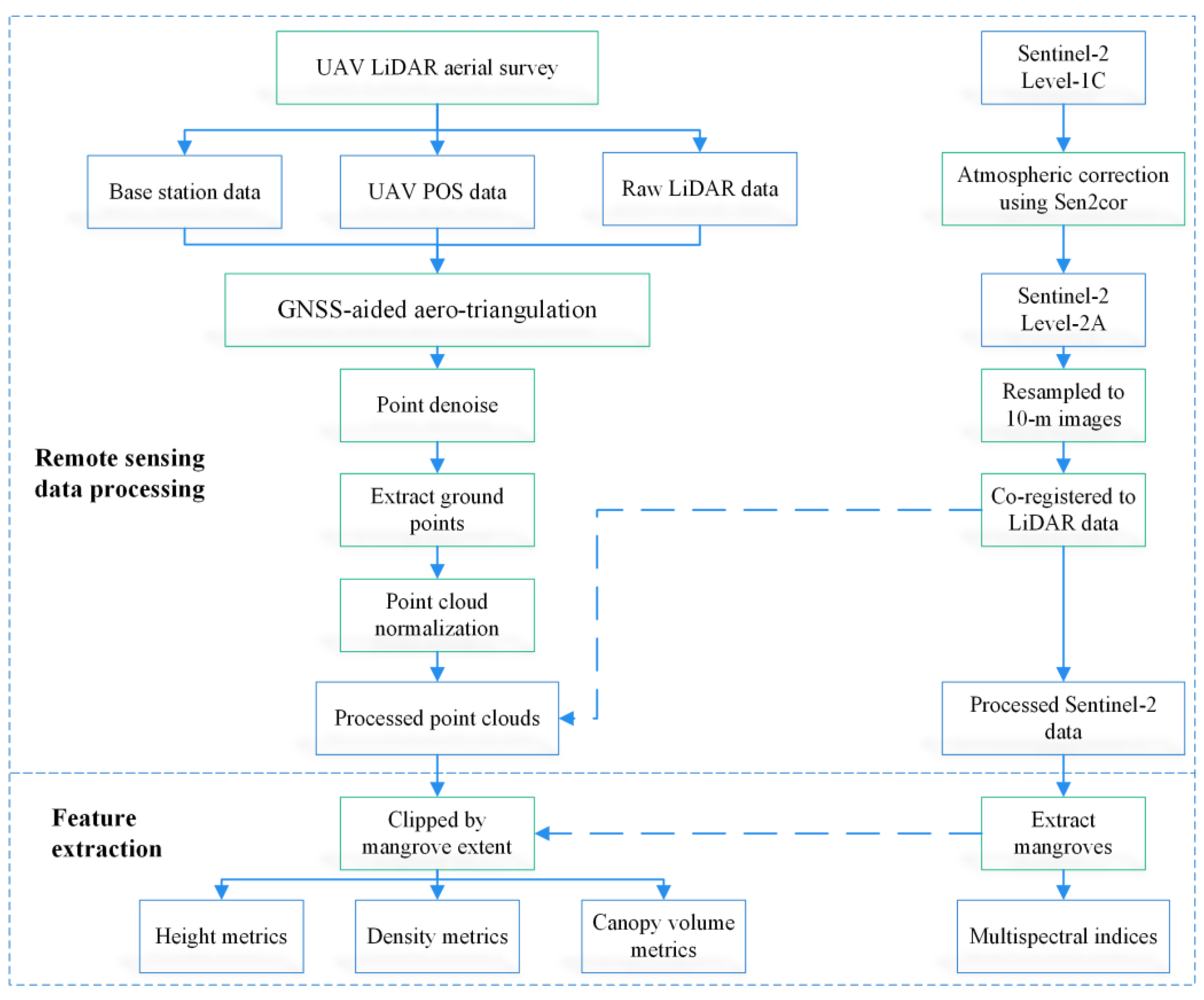
The UAV-LiDAR point clouds were obtained by a Velodyne VLP-16 Puck sensor mounted on a DJI M600 UAV on 25–28 March 2018. This laser sensor has 16 scanning channels and operates at 903 nm wavelength, which can produce up to 300,000 points per second. We conducted 16 flights in the study area with a flight altitude of 52 m, a flight speed of 5 m/s, and an average swath width of 110 m. The UAV flight times were selected in low- or middle-tide period. Overall, the mean point density of all collected LiDAR data was 94 points/m2. Figure 2 describes the workflow of UAV-LiDAR data processing. The main processing steps for point clouds included GNSS-aided aero-triangulation, point denoise, ground point extraction and point cloud normalization (Figure 2). The GNSS-aided aero-triangulation was used to calculate the accurate geographical positions of point clouds based on base station location data and POS (position and orientation system) data, which was conducted in POSPac UAV 8.1 software (Applanix, Richmond Hill, Ontario, Canada). The point denoise was utilized to filter noise points that are located above and below the mangrove forests, which was done by using the Remove Outliers tool and the Noise Filter tool in LiDAR360 software (GreenValley, Being, China). Following the point denoise, the point clouds were classified as ground and non-ground points using an improved progressive TIN (triangulated irregular network) densification filtering algorithm [36]. The ground points were further inspected and edited in manual. The final ground point density was 62 points/ha. Then, these ground points were used to produce a digital elevation model (DEM). A digital surface model (DSM) was also produced based on all point clouds. Finally, to eliminate the influence of ground terrain on point clouds, the non-ground points were normalized by the DEM in LiDAR360 software. For detailed descriptions of the last three steps, refer to the LiDAR360 User Guide (http://greenvalleyintl.com/software/lidar360/).
2.3. Sentinel-2 Data
We downloaded eight Sentinel-2 images from the Copernicus Open Access Hub (https://scihub.copernicus.eu/) to cover the entirety of Hainan Island depicted in Figure 1. Because the original imagery was Level-1C product, namely, orthorectified top of atmosphere reflectance data, it needed to be calibrated to a Level-2A product, namely, bottom-of-atmosphere reflectance data. This atmospheric correction was implemented using the Sen2Cor atmospheric correlation processor (version 2.5.5). The other key processing steps included resampling and co-registering to LiDAR data. The procedure for processing Sentinel-2 data is portrayed in Figure 2.
3. Methods
3.1. LiDAR Metrics and Sentinel-2 Indices
Few studies have used high-density LiDAR point clouds to estimate mangrove AGB, and few studies have reported the most important LiDAR metrics for predicting mangrove AGB [13,14]. A total of 53 LiDAR metrics were derived preliminarily (24 for height, 12 for density, and 17 for canopy volume) [14,37], as presented in Table A1 [14,38,39,40]. A novel canopy thickness metric (CTHK) was created and used to describe the thickness of mangrove canopy based on the analysis of UAV-LiDAR point clouds [41]. In each field plot, the 53 LiDAR metrics were extracted. All of the LiDAR point clouds were first tessellated into grids with a cell size of 10 × 10 m with the same original point as that of the Sentinel-2 imagery. Subsequently, the 53 LiDAR metrics were computed for each cell.
A total of 32 Sentinel-2 multispectral indices, presented in Table A2, were selected on the basis of their previous performance in studying mangroves and terrestrial forests. The indices consisted of 10 original Sentinel-2 bands, 7 conventional near-infrared indices, 12 red-edge indices, and 3 shortwave infrared indices.
3.2. Mangrove Extent Extraction
Prior to mapping mangrove height and AGB, the mangrove extent on Hainan Island needed to be extracted. We applied a combination of object- and pixel-based methods for mangrove extent classification using Sentinel-2 imagery. Firstly, an object-based decision tree classification method [42] was implemented for the processed Sentinel-2 imagery to discriminate mangroves from water, terrestrial vegetation and other lands (including construction land, mudflat and bare land). This process was conducted in eCognition 9.0 (Trimble, Sunnyvale, CO, USA) and multi-resolution segmentation was utilized with a scale of 30 in accordance with our previous study on Hainan Island [43]. Then, these candidate mangrove patches were visually examined one by one in high spatial resolution imagery from Google Earth; the examination was carried out by two mangrove researchers who had approximately 10 years of mangrove research experience. During the process, false patches were deleted or edited, and the underestimated mangroves were added manually in eCognition 9.0. Subsequently, the mangrove pixel cells with an FDI (forest discrimination index) [44] higher than 200 were eliminated to exclude non-vegetation (such as mudflats) and grass from the set of mangrove objects. Finally, a thematic map of the mangrove extent on whole Hainan Island was obtained.
3.3. Model Fitting Based on LiDAR Samples
In this study, LiDAR sampling involved a series of LiDAR transects acquired over an area of interest and used as samples. Then, the established procedures from field sample-based forest inventories are adapted and applied to the LiDAR samples [15], which means the LiDAR samples are used in a similar manner to field samples.
Since the point cloud density in the 20 m distance off the UAV flight strip centerlines is more uniform, only the LiDAR grid cells in this 40 m range were used as LiDAR plot samples. We finally obtained 14,628 candidate LiDAR samples with size of 10 ×10 m.
3.3.1. Height Estimation Model
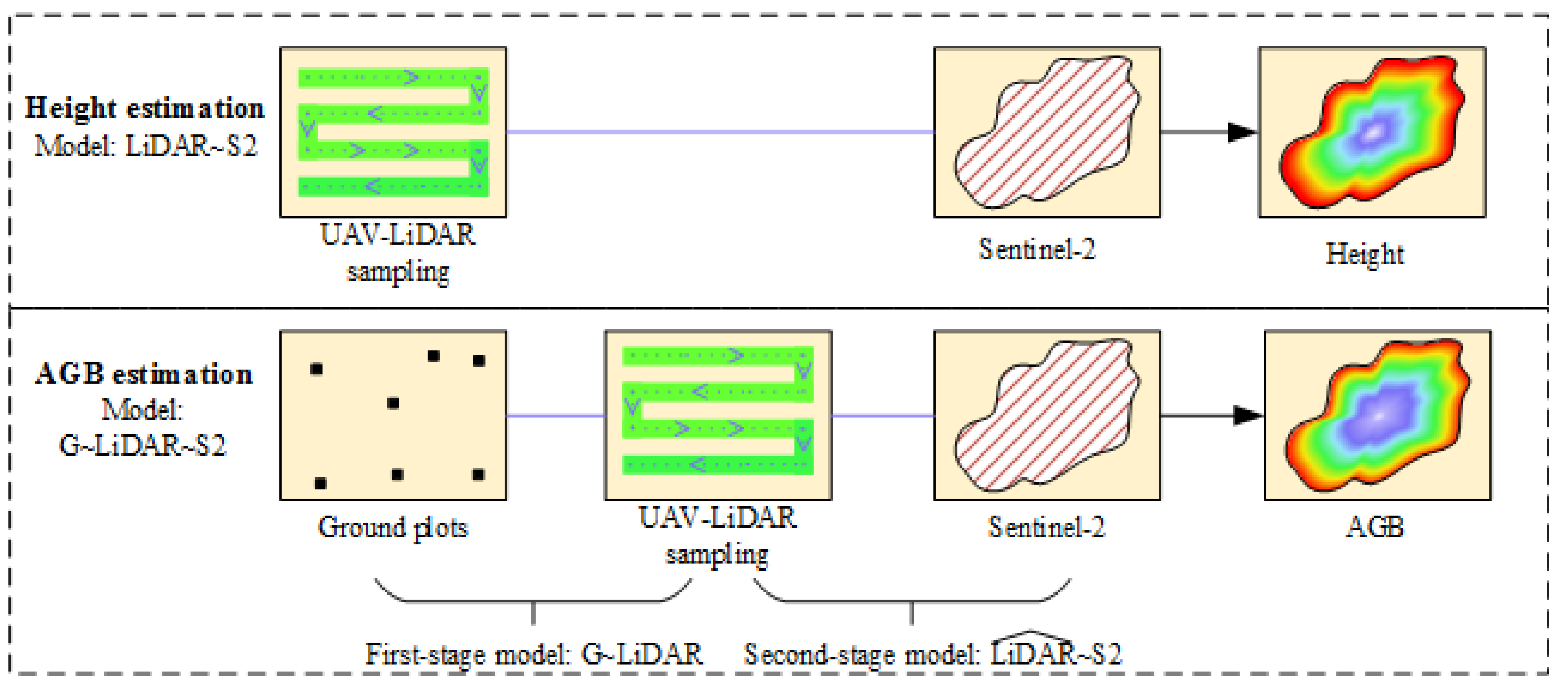
UAV-LiDAR data have high-density point clouds and can obtain mangrove heights with high accuracy [45]. Therefore, the canopy heights of the partial-coverage UAV-LiDAR grid cells were directly used as reference data for Sentinel-2 data to fit a height prediction model (top graph in Figure 3). The canopy heights were derived by subtracting the DEM from the DSM. The Sentinel-2 features were used as explanatory variables. The constructed height estimation model was named LiDAR~S2 (top picture in Figure 3).
3.3.2. AGB Estimation Model
To estimate AGB, we first constructed a model, named G~LiDAR, to link ground plot AGB with coinciding UAV-LiDAR point clouds (clipped by the polygon of the field plot) and then obtained UAV-LiDAR-estimated AGB. In this process, the field estimated AGB was used as response data and the UAV-LiDAR metrics were used as explanatory variables. Then the G~LiDAR model was applied to the 14,628 LiDAR plot samples to obtained the AGB of these LiDAR grid cells.
Subsequently, the UAV-LiDAR-estimated AGB values of the LiDAR grid cells were used as reference data for the wall-to-wall Sentinel-2 data to fit a retrieval model, named , in which the Sentinel-2 features were used as explanatory variables. The overall model of the two stages for mangrove AGB estimation was named G~LiDAR~S2 (bottom graph in Figure 3).
In addition, the traditional method, which directly relates field estimated AGB with the coinciding Sentinel-2 data by a statistical model (named G~S2), was also constructed as a benchmark in this study.
3.4. Random Forest and Feature Selection
The random forest (RF) algorithm was employed for all mangrove height and AGB estimation models in this study due to its good performance of building prediction models [46,47]. RF regression first builds a large number of decision trees and then averages the prediction values of all trees to obtain the final estimates [48]. There are two important parameters when building an RF model: ntree and mtry. The ntree parameter determines the maximum number of created decision trees, while the mtry parameter control the number of features that are randomly selected to compute the best split at each node of each decision tree. In this study, we set the value of ntree to 5000, which is big enough for error to become convergent, and set the value of mtry to the default value, namely the square root of the total number of input features.
The RF algorithm can also evaluate the importance of input variables by using out-of-bag (OOB) samples through a random permutation method. The increase of mean square error (MSE) from the changed OOB samples are compared with the original MSE of OOB samples, and then a metric %IncMSE (the percentage increase in the mean square error) is obtained and used to quantitate the importance of each predictor variable [12]. The OOB samples are mainly utilized to assess the accuracy of the newly fitted RF model. The detailed process of how the RF algorithm measures feature importance was described by Breiman [48], and a specific application was presented by Pham and Brabyn [12].
Usually, a model constructed from a small number of predictor variables is more interpretable and eliminating irrelevant and highly correlated variables may improve the predictive power [49]. Therefore, prior to building the final prediction models, an RF-based backward feature elimination method was utilized to optimize the feature space for each model [12,50]. The method compared the cross-validated prediction results of RF models, and 10% of variables were eliminated at a time. When the cross-validation error of a set of features was within one standard deviation of the minimum cross-validation error, and when the number of this feature set was at a minimum, this group of features was considered to be the set of optimal predictor variables. In this study, the R package was used to implement the backward feature elimination method, which was replicated 20 times, with 5-fold cross-validation, to get the optimal variables [50].
3.5. Accuracy Assessment
The classification accuracy of mangrove extent was assessed by the overall classification accuracy (OA), the producer’s accuracy (PA), and the user’s accuracy (UA) using a classification confusion matrix [51]. Since we focused on mangrove extent extraction, when assessing classification accuracy, other land cover classes such as water, terrestrial vegetation, construction, and bare lands were all merged as “non-mangroves”. Two-hundred points per class (mangroves and non-mangroves) were randomly generated and used to assess mangrove identification accuracy.
For mangrove height and AGB estimation accuracy assessments, the coefficient of determination R2, root-mean-square-error (RMSE), and RMSE expressed as a percentage of the observed mean (RMSE%) were employed [10,12]. Specifically, 4281 randomly selected LiDAR plots (10 × 10 m) were used to calibrate and validate the height estimation model. Of the 4281 LiDAR plots, 2/3 of them were used for training and 1/3 were used for validation.
For the first-stage AGB estimation model (G~LiDAR), of the 97 field samples, 62 samples inside the UAV-LiDAR coverage area were used for training, and accuracy was assessed by the 10-fold cross-validation method. The accuracy of the second-stage model () was assessed by independent validation samples, namely the other 35 field samples (24 samples are outside the UAV-LiDAR coverage area and the other 11 samples were randomly selected form the QPR), by comparing the predicted and observed values. The same independent sample validation method with the 35 field plots was also utilized to examine the accuracy of the traditional approach (the G~S2 model).
4. Results
4.1. Mangrove Identification Result
This study estimated that there is a total of 3697.02 ha of mangrove forests on Hainan Island. The overall classification accuracy of mangroves and non-mangroves was 98.00% (Table 2). The user’s accuracy of mangroves was 96.50%, while the producer’s accuracy was slightly higher, with an accuracy of 99.48%. The mangroves were mainly distributed among six sites, namely, Dongzhai Harbor, Qinglan Harbor, Danzhou Bay, Meilang Harbor, Xinying Harbor, and Sanya River, and dispersed in 3782 patches with a mean path area of approximately 1 ha.
4.2. Feature Selection
The feature selection results are presented in Table 3, and the feature elimination processes are portrayed in Figure 4. There were six features selected in the LiDAR~S2 model for mangrove height estimation. Among these six features, four were selected from the shortwave infrared bands or their derived indices. The other two were the blue band and the MTCI (the MERIS terrestrial chlorophyll index) computed from red-edge bands.
For the first-stage G~LiDAR model for AGB estimation, 11 LiDAR metrics were chosen from the initial 53 metrics. Most of them were height metrics, while two were canopy volume metrics (CC1.3 and CTHK) and one was a density metric (D01). A total of 12 features were selected for the second-stage model : half of them were from red-edge bands, and five features were from shortwave infrared (SWIR) bands or their derived indices. For the traditional model G~S2, 14 features were selected. In addition to the nine red-edge and SWIR bands, the red, green and blue bands and two traditional indices were also selected.
4.3. Model Assessment
The calibration and validation accuracies of the height and AGB estimation models are presented in Table 4. To compare the mean and distribution of the mangrove height and AGB values, boxplots of the observed and predicted values from the height estimation model (LiDAR~S2) and the AGB estimation model () are presented in Figure 5A. The residual errors between observed and predicted values were determined using independent validation samples and are plotted in Figure 5 for the height and AGB models, respectively.
4.3.1. The Height Estimation Model
As a mangrove height model, the LiDAR-S2 model performed well, with an R2 of 0.67 and an RMSE of 1.90 m. Figure 5B reveals that some low height points were overestimated, while underestimation occurred for high height points greater than 15 m. Figure 5A also reflects this phenomenon. Therefore, tree height obtained from the estimation by UAV-LiDAR has an overestimate bias in low tree and an underestimate bias in high tree. Meanwhile, the mean and distribution of the observed height are similar to those of the predicted height overall.
4.3.2. The First-Stage Model of AGB Estimation
The first-stage G~LiDAR model for mangrove AGB prediction produced relatively high explanatory power, with an R2 of 0.78 and an RMSE of 42.29 Mg ha−1 (Table 4), which indicates that the UAV-LiDAR data accurately predicted mangrove AGB.
4.3.3. The Second-Stage Model of AGB Estimation
In the second stage, the model linking the first-stage AGB prediction with Sentinel-2 variables produced an R2 metric of 0.62 and an RMSE of 50.36 Mg ha−1, which represents greater explanatory power compared with the traditional G~S2 model (R2 of 0.52 and RMSE of 56.63 Mg ha−1).
The analysis of the residual plots (Figure 5C,D) shows that the residual error variation range of the G~LiDAR~S2 model was smaller than that of the G~S2 model. Both the LiDAR sampling method and the traditional method underestimated high AGB (greater than 250 Mg ha−1), but this phenomenon was more obvious in the G~S2 model. The boxplots of the field estimated and predicted AGB of model reveal that the upper and lower quartiles of the two data are similar, but the maximum and minimum AGB of the predicted values are less than those of the field estimated values. Overall, UAV-LiDAR sampling could scale up mangrove AGB estimation and appeared to improve prediction accuracy.
4.4. Mangrove Height and AGB Map of Hainan Island
The resultant mangrove height and AGB maps of Hainan Island are presented in Figure 6 and Figure 7, respectively. The summaries of mangrove height and AGB in different districts of Hainan Island are shown in Table 5.
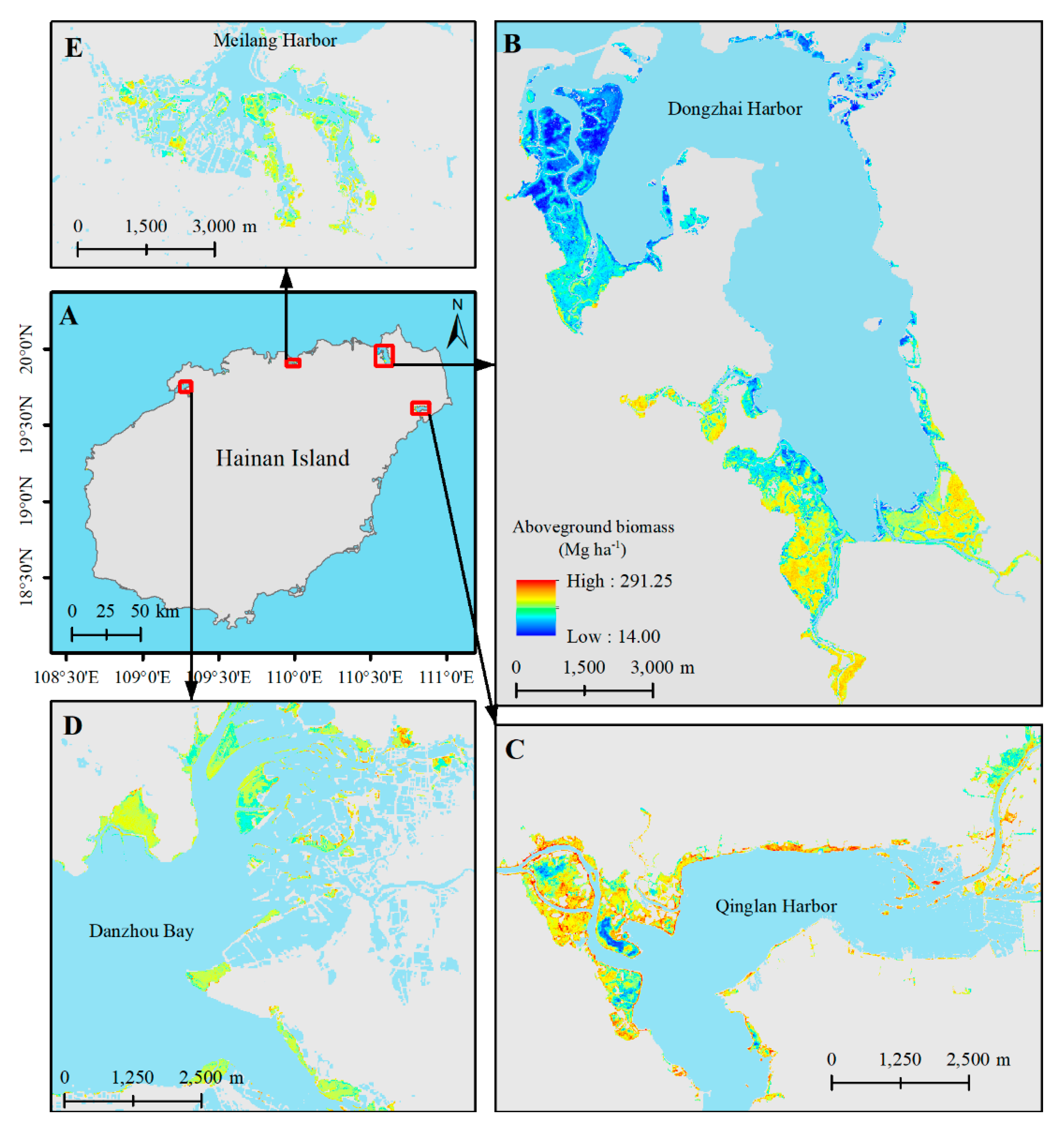
The mean height of the mangrove forests on Hainan Island was 6.99 m with a standard deviation of 2.14 m. There were three districts whose mangroves had a mean height of over 8 m—Wenchang, Dongfang and Qionghai. The mangrove area of Wenchang was the largest, and the mangrove areas of the other two districts were less than 100 ha. In Figure 6C, the yellow and red colors show that the height of most of the mangroves in Qinglan Harbor (Wenchang) was higher than 8 m. The dwarf mangroves, indicated by dark blue, were mainly distributed in the north of Dongzhai Harbor (Haikou), which results in the lowest average tree height of mangroves in Haikou (5.93 m).
The total mangrove AGB on Hainan Island was 474,199.31 Mg, with a mean AGB of 128.27 ± 45.87 Mg ha−1. The mangrove AGB hot spots mainly lay in Qinglan Harbor and the south of Dongzhai Harbor. Although areas with high AGB were found in other places, such as Danzhou Bay (Danzhou) presented in Figure 7D, their area was small with a scattered distribution. Among the nine districts, the mangroves of Wenchang, Dongfang and Qionghai had the highest AGB density, while the mangroves of Haikou had the lowest mean AGB of 106.47 Mg ha−1. In addition, a comparison of the mangrove height and AGB maps reveals that they are similar: that is, the high (low) height area is also a high (low) AGB area.
4.5. Variable Importance
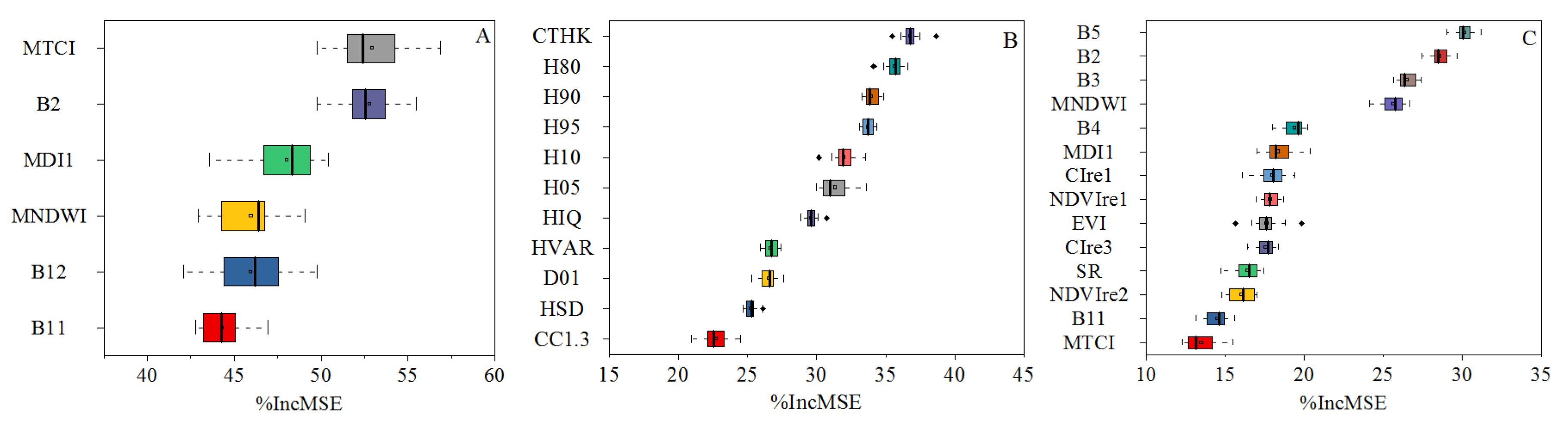
The importance of each predictor variable for the height (LiDAR~S2) and AGB estimation models (G~LiDAR and G~S2) is illustrated in Figure 8. Since the second-stage model for AGB estimation was an indirect model and its training samples were secondhand data, the importance of the input features in this model was not measured.
Figure 8A shows that the MERIS terrestrial chlorophyll index derived from red edge bands and blue Band 2 were the two most important features for mangrove height estimation. The mangrove discrimination index 1 and the modified normalized difference water index ranked third and fourth in importance, respectively. The two indices were computed from shortwave infrared Band 11.
Figure 8B indicates that the newly created canopy thickness metric was the most important LiDAR metric for predicting mangrove AGB. The LiDAR indices that describe the characteristics of the upper canopy (H80, H90, H95) ranked second in importance, while the H10 and H05 metrics describing bottom canopy characteristics ranked third for mangrove AGB estimation. The HVAR and HSD metrics, which characterize the mangrove canopy variation, ranked last among these selected features, along with the density metric D01 and the canopy coverage index CC1.3.
Figure 8C shows that red-edge Band 5 was the most important feature for estimating mangrove AGB among all Sentinel-2 original bands and multispectral indices. The red, green, and blue bands also ranked among the top five. Although there were six red-edge features selected and only three SWIR features chosen, the MNDWI (Modified Normalized Difference Water Index) and MDI1 (Mangrove Discrimination Index 1) calculated from SWIR ranked higher than the five red-edge-derived indices. Overall, among the five red-edge vegetation indices, the importance of CIre1 and CIre3, which are used for chlorophyll estimation, was greater than that of NDVIre1 and NDVIre2. The two selected conventional near-infrared vegetation indices SR and EVI ranked lower.
5. Discussion
This study presents the first mangrove height and AGB map of Hainan Island obtained by a novel UAV-LiDAR sampling method with Sentinel-2 imagery as auxiliary data. This study is also the first to use high-density UAV-LiDAR point clouds to retrieve mangrove biophysical parameters [13]. Hainan Island has the most species diverse mangrove forests in China, and nearly 95% of Chinese mangrove species communities have been found on Hainan Island [8]. Therefore, maps are practical and urgently needed to estimate Hainan Island’s mangrove height and AGB and provide the first mangrove forest structure. We anticipate that the 10 m spatially resolved mangrove height and AGB maps of Hainan Island could motivate further studies of Chinese mangroves and provide insights into mangrove protection and management [52]. We also anticipate that these maps will be used as baseline data for future studies of mangroves’ response to climate warming and sea level rising in this region. The UAV-LiDAR sampling method increases the distribution and sample size of local data to inform on stand structure to estimate and map mangrove height and AGB [10]. The successful application of the G~LiDAR~S2 model at the regional scale (the entire Hainan Island) is also a major operational advance in estimating and mapping mangrove structure over large areas.
5.1. The Mangrove Height and AGB on Hainan Island and Comparison with Mangroves in Other Areas
Mangrove height and biomass are related to geographical location, species composition and structure, water-heat conditions, community development status, and external disturbances. The average mangrove height on Hainan Island is 6.99 ± 2.14 m, which is significantly higher than other Chinese mangroves, such as the mangroves in Zhangjiang estuary, Fujian province (mean height 3.1 m) [53], and Dandou Sea coast, Guanxi province (mean height < 3.5 m) [45]. The reason may be that the latitude of mangroves on Hainan Island (18°–19°N) is lower than the latitude of mangroves in other places in China (21°–28°N) [54,55]. Another explanation for this is that the tall mangrove species B. sexangula and Sonneratia spp. (usually taller than 8 m) only grow on Hainan Island [7], and B. sexangula is one of the dominant species in the south of Dongzhai Harbor and Qinglan Harbor, covering a large number of areas. For the other seven major mangrove species on Hainan Island, the height of R. stylosa, K. candel, R. apiculata, and E. agallocha is usually 4–8 m, while the height of C. tagal, L. racemosa, and A. marina is usually lower than 3 m. The low height range covers a great number of mangrove species in the study area, which may result in the underestimate bias in low trees. While, the underestimate bias of high trees may be attributed to the radiometric saturation effect of Sentinel-2 imagery [19].
Previous studies have portrayed mangrove tree height as directly related to AGB [56,57]. Saenger and Snedaker [58] even provided a global scale allometric equation that links tree height with AGB for mangrove forests: AGB (Mg ha−1) = 10.8 × H(m) + 35. Therefore, the mangrove AGB density on Hainan Island should greater than the mangrove AGB density in other regions of China. This inference is supported by comparisons between the predicted mangrove AGB on Hainan Island and the reported mangrove AGB in other sites in China. For example, Wang et al. [59] reported a mangrove AGB of 79 Mg ha−1 in Jiulong River Estuary, Fujian, China and Jiang et al. [60] reported a mangrove AGB density of 54.81 Mg ha−1 in Shenzhen Bay, Guangdong, China. They were all lower than the mean AGB of the mangroves on Hainan Island (128.27 Mg ha−1).
The average height of Hainan Island’s mangroves (6.99 m) is higher than the mean height of mangroves (~5.0 m) in the Everglades National Park, Florida, USA, reported by Simard et al. [56], and greater than the mean height of mangroves (3.2 m) reported by Hickey et al. [61] in northwest Australia. However, they are lower than the average height of mangroves (7.5 m) reported by Fatoyinbo and Simard [62] for all of Africa and significantly lower than the mangrove mean height (~21 m) in Papua, Indonesia, given by Asian et al. [3]. A similar trend is found by comparing the mangrove AGB in these four places with the mangrove AGB on Hainan Island. The mangrove AGB density on Hainan Island (128.27 Mg ha−1) is higher than the mangrove AGB density (38.77 Mg ha−1) in the Everglades National Park, Florida, USA [56], greater than the mangrove AGB density in northwest Australia (70 Mg ha−1) [61], and slightly higher than the mean mangrove AGB (116 Mg ha−1) on the African continent [62]; however, it is significantly lower than the mangrove AGB density in Papua, Indonesia (292.72 Mg ha−1) [3]. These discrepancies could be attributed to differences in geographical location, climate, and species composition. For example, in the Everglades National Park, scrub forests are widely distributed on internal coasts as well as inland, and this park is located at 25° N, which is higher than the latitude of Hainan Island (18–20° N).
To date, no global mangrove height map has been published. The reported global mangrove AGB density of 184.8 Mg ha−1 was deduced by a climate-based model and not from remote sensing surveys [54]. However, we can infer that the mean height and mean AGB of the mangrove forests on Hainan Island are higher than the mean height and mean AGB of the majority of other mangroves in China and lower than the global mean height and AGB of mangrove forests. The height inference is based on the comprehensive consideration of the global mangrove distribution [63], climate [54], and mangrove species composition [64]. If we substitute the global mangrove AGB density value of 184.8 Mg ha−1 into the global equation of AGB (Mg ha−1) = 10.8 × H(m) + 35, we can deduce that the global average height of mangrove forests is about 13.87 m, which is higher than the mean mangrove height on Hainan Island.
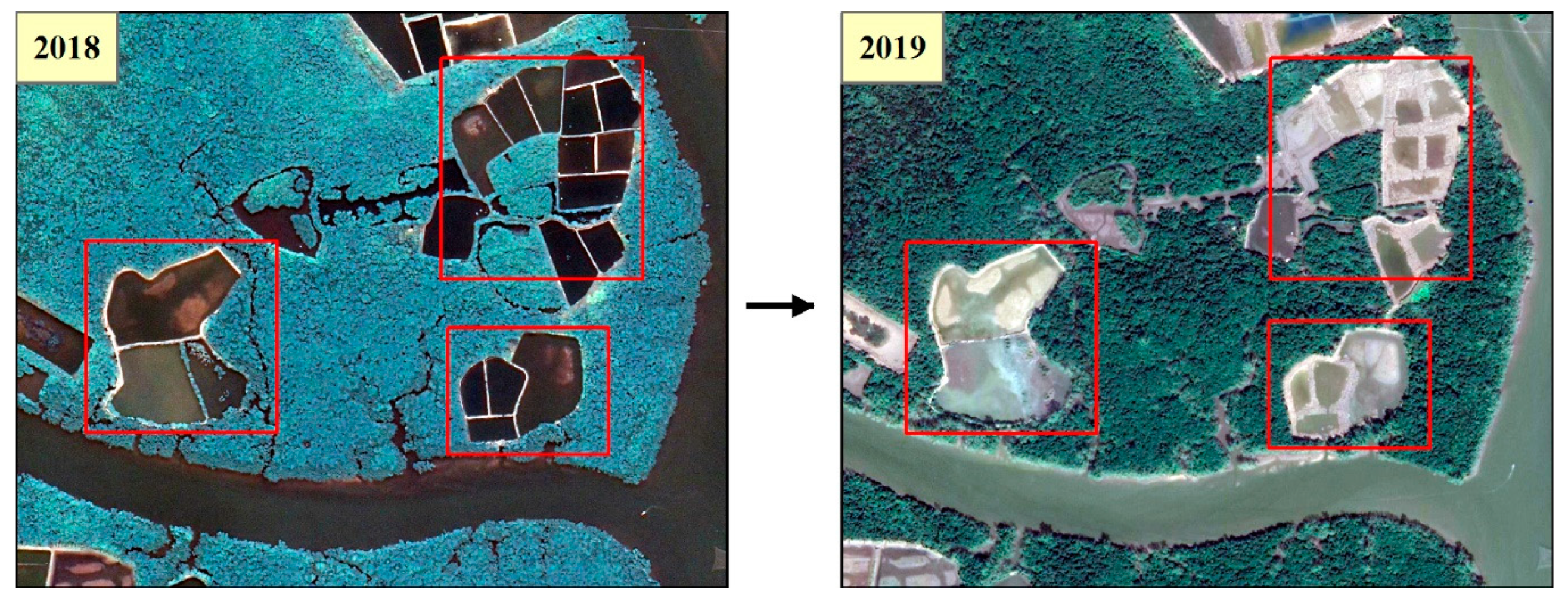
Consequently, the obtained height and AGB maps of mangrove forests on Hainan Island are useful. Firstly, they could provide an opportunity to address mangrove restoration problems and provide insights into the dynamics of mangrove recovery. For example, a mangrove reforestation plan has been widely implemented on Hainan Island in order to restore and rehabilitate mangrove forests (Figure 9). Secondly, the maps could serve as a baseline for future mangrove studies, such as the mangrove response to hurricanes and sea level rise.
5.2. Fieldwork Challenges in Mangrove Habitats and the Feasibility of LiDAR Sampling
Previous studies have always mentioned the great difficulty of fieldwork in a mangrove habitat [3,13]. Because of the mudflat and shallow seawater environment, investigators cannot walk in most mangrove habitats with outdoor shoes, which become struck in the mud, but have to be barefoot or wear long rain-shoes. For example, while field sampling mangroves on Hainan Island, we often walked barefoot (Figure 10A). Hence, it was easy to suffer arm and leg injuries due to mangrove branches and roots or shells and oysters in the water. Furthermore, since mangroves are distributed in tropical and subtropical regions, there are many mosquitos in mangrove forests all year round. In the field survey of mangroves on Hainan Island, investigators were sometimes bitten by mosquitoes more than 20 times a day. In addition, because of the high density of the forests and the aerial and prop roots at the bottom, it is difficult for investigators to walk through mangrove forests (Figure 10). These factors make fieldwork in mangrove habitats more challenging than fieldwork in terrestrial forests. The great difficulty of fieldwork in mangrove forests is also one of the reasons that key research topics in mangrove remote sensing have lagged behind key research topics in terrestrial forests, as concluded by Wang et al. [13], who conducted a comprehensive review of the mangrove remote sensing studies conducted over the past sixty years. This may also explain the lack of a thematic AGB map of mangroves produced by remote sensing techniques to date.
This study proposes a UAV-LiDAR sampling method for estimating mangrove height and AGB to overcome the challenges of fieldwork in mangrove habitats. UAV-LiDAR can characterize mangrove morphology with a finer spatial resolution [20,45]. In addition, UAV-LiDAR is more flexible than airborne and satellite LiDAR because it can work on any low-wind day with arbitrary time intervals. This flexible and operational characteristic makes UAV-LiDAR very suitable for sampling elongated patches of mangroves. The good accuracy (height: R2 = 0.67, RMSE% = 26.24%; AGB: R2 = 0.62, RMSE% = 35.41%) obtained from the UAV-LiDAR sampling method (height: LiDAR~S2 model; AGB: G~LiDAR~S2 model) in this study also demonstrates the feasibility of UAV-LiDAR sampling for mangroves (Table 4).
The derived AGB estimation accuracy is similar to the accuracy (R2 = 0.62, RMSE% = 40.00%) reported by Pham and Brabyn [12] who used spectral bands, vegetation indices and texture of 10 m SPOT-5 imagery. Considering that their study area only has three floral association types and that Hainan Island has more than nine main mangrove communities, our estimation accuracy is satisfying. Compared with the AGB prediction accuracy (R2 = 0.55, RMSE% = 47.07%) reported by Asian et al. [3], the accuracy produced by the G~LiDAR~S2 model is higher. However, the AGB accuracy in this study is lower than the accuracy (R2 = 0.82–0.84, RMSE% = ~43%) reported by Castillo et al. [23] using Sentinel-1/2 imagery and lower than the accuracy (R2 = 0.80–0.88, RMSE% = 23–33%) reported by Fatoyinbo et al. [5] using wall-to-wall airborne LiDAR data. The former could be attributed to the study area of Castillo et al. [23] being dominated by one mangrove genus, namely, Rhizophora, which means that the forest structure is relatively simple compared with Hainan Island’s diverse mangrove forests. The latter is likely to be related to the data difference and retrieval unit of the map. Fatoyinbo et al. [5] used full-coverage LiDAR data with a point density of 10 points/m2, and their estimation unit was 25 m. In our study, the UAV-LiDAR data was just partial coverage, with Sentinel-2 multispectral imagery used as wall-to-wall auxiliary data, and the calculation unit was 10 m. When directly linking the field plots with the UAV-LiDAR data (G~LiDAR model) in our study, relatively high accuracy is produced with R2 = 0.78–0.80 and RMSE% = 28–29%. In addition, for heterogenous mangrove forests, large statistical units may improve prediction accuracy but reduce detail information [14]. Therefore, these findings prove that UAV-LiDAR is feasible for mangrove sampling.
There is uncertainty in the height (LiDAR~S2) and AGB estimation models (G~LiDAR~S2) based on LiDAR sampling. For the LiDAR~S2 model, the uncertainty is mainly from LiDAR plot sampling and model fitting, which is similar to the uncertainty of the two-phase hybrid inference using partial-coverage UAV data for the forest volume estimation reported by Puliti et al. [16]. Concerning to the G~LiDAR~S2 model, its uncertainty includes the uncertainty of two stages, namely G~LiDAR and . The first-stage G~LiDAR is model-based inference [15,16]. When field samples are collected according to probabilistic principles, its uncertainty is mainly from model fitting. Pereira et al. [14] discussed how to reduce uncertainty in mapping mangrove AGB using field plots and airborne LiDAR data. The second-stage belongs to hybrid inference [19,65]. Its uncertainty is not only caused by LiDAR plot sampling and model fitting but also by error propagation from the first-stage estimated AGB values. In addition, our study employed the non-parameter RF regression to fit models. The uncertainty of LiDAR sampling-based model is an important issue for future research. Réjou-Méchain et al. [66] presented several caveats when using very high spatial resolution products to bridge field plots and large-scale remote sensing data. They also analyzed the sources of error and discussed ways to reduce these errors in the process of upscaling forest biomass from field to satellite measurements. Regarding to model fitting error, the deep learning-based retrieval model may be an alternative to the RF model in the future [67].
5.3. Relevance of Predictor Variables
Because there is a lack of accurate training data for mangrove height, few studies have used passive remote sensing data to estimate mangrove height [13]. Therefore, the spectral bands that are important for mangrove height inversion are not yet clear. This study presents the first attempt to invert mangrove height using Sentinel-2 data. The results for the importance of the variables show that the red-edge derived MERIS (Medium Resolution Imaging Spectrometer) terrestrial chlorophyll index (MTCI) plays the most important role in predicting mangrove height. The MTCI is correlated strongly with red-edge bands but, in contrast to red-edge bands, is sensitive to high values of chlorophyll content [68]. Pastor-Guzman et al. [69] also demonstrated that the MTCI is highly correlated with mangrove chlorophyll concentration. Meanwhile, taller mangrove forests on Hainan Island usually have denser branches and leaves, which could indicate a higher chlorophyll concentration. It is difficult to explain the second-ranking of the blue band, but its considerable importance was also shown in a mangrove AGB retrieval study using WorldView-2 imagery [70] and a terrestrial forest growing stock volume prediction study utilizing Sentinel-2 imagery [21]. The SWIR bands are low-reflectance bands compared with near-infrared bands and are sensitive to the leaf structure and water content of plants. Thus, mangroves show a low spectral reflectance in the SWIR bands that varies according to the amount of water content in different mangrove species. This may explain why the SWIR features play important roles in mangrove height estimation. In addition, the importance of these SWIR features may be related to the fact that tall mangroves are distributed in middle- and low-tide zones and closer to hydrological features than dwarf mangroves, such as the creek entrance in Dongzhai Harbor (Figure 7B) and the river in Qinglan Harbor (Figure 7C).
Of the Sentinel-2 features for mangrove AGB prediction, the red-edge 1 and SWIR 1 bands, along with their derived indices, are the highest in terms of importance when considering both the ranking and the number of features, thus confirming the results reported by Zhu et al. [70] and Castillo et al. [23]. Usually, a slight change in vegetation properties (such as leaf structure, chlorophyll content, and leaf pigments) leads to an obvious shift in the red-edge spectral curve [71], which may explain why red-edge features are incredibly important for predicting mangrove AGB. The reasons for the significant importance of the SWIR 1 features in mangrove AGB prediction are similar to those of the importance of SWIR features in mangrove height estimation. In addition, Wang and Sousa [72] also proved that wavebands in the red-edge (780, 790 and 800 nm) and SWIR (1480, 1530 and 1550 nm) bands are the most informative bands for mangrove species discrimination. Mangrove AGB is also correlated with mangrove species [11,29]. The higher ranking of the blue, green and red bands are in line with what was observed by Zhu et al. [70], Mura et al. [21], and Pham and Brabyn [12]. The higher rankings may also partly be explained by their higher spatial resolution of 10 m compared with other multispectral bands of Sentinel-2 imagery (20 or 60 m), except for the near-infrared Band 8.
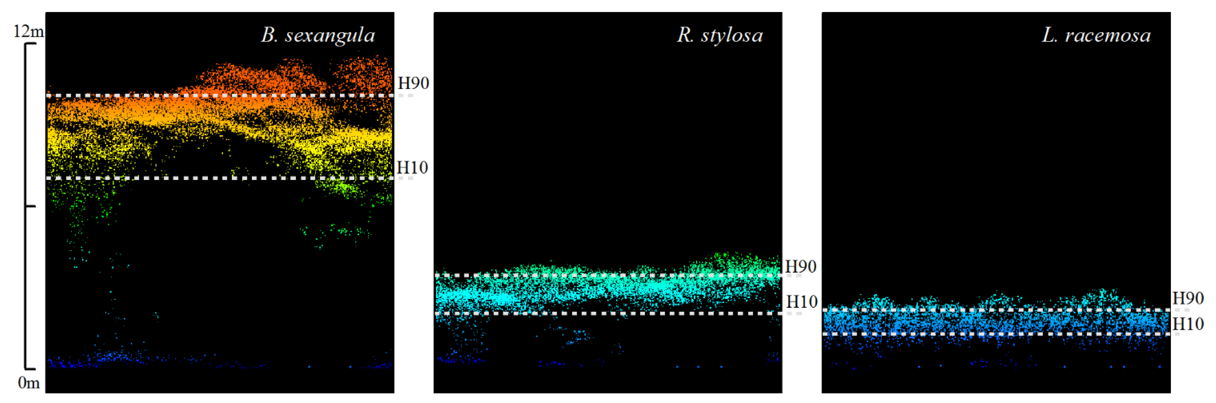
Of the UAV-LiDAR metrics, the newly created canopy thickness metric is the most important predictor variable. Given the weaker penetration ability of UAV-LiDAR (limited by the loading capacity of the UAV platform) compared with airborne LiDAR, the pulse beam emitted by UAV-LiDAR may not penetrate a very dense canopy and detect specific branches. Nonetheless, UAV-LiDAR could still capture the canopy thickness of mangroves, and the taller AGB mangroves usually have thicker canopies (CTHK = H90–H10). Figure 11 illustrates the profiles of three dominant mangrove species on Hainan Island on UAV-LiDAR point clouds. The canopy thickness of B. sexangula, R. stylosa and L. racemosa is 3.06, 1.40, and 0.89 m, respectively, with the AGB density of 215.20, 110.36, and 62.83 Mg ha−1. This also explains why the LiDAR metrics that characterize the upper canopy (H80, H90, H95) and the bottom canopy (H05, H10) are found to be important for mangrove AGB estimation in this study, which is consistent with the results of Fatoyinbo et al. [5], Pereira et al. [14], and Hickey et al. [61], who demonstrated the crucial importance of the LiDAR metrics that characterize the upper canopy for mangrove AGB prediction. The last four LiDAR metrics include two metrics describing the point cloud variation (HVAR and HSD), one density metric (D01), and one canopy cover index (CC1.3). The sensitivity of the HVAR and HSD in this study are in accordance with what was observed by Owers et al. [40] in a mangrove AGB study using terrestrial LiDAR. Consequently, we can infer that the canopy thickness is the most important LiDAR metric for mangrove AGB estimation, followed by upper canopy height metrics, bottom canopy height metrics, and point cloud variation metrics, in that order.
6. Conclusions
This study presents the first mangrove height and aboveground biomass (AGB) maps of Hainan Island using a novel UAV-LiDAR sampling method with Sentinel-2 imagery as auxiliary data. From UAV-LiDAR sampling, we constructed the LiDAR-S2 and G~LiDAR~S2 models for mangrove height and AGB estimations based on random forest regression, respectively. The LiDAR~S2 height model uses LiDAR plots as training samples and links the UAV-LiDAR observed height with Sentinel-2 data. The G~LiDAR~S2 AGB model utilizes the transect-based UAV-LiDAR data as intermediate data to transfer AGB from field plots to wall-to-wall Sentinel-2 data.
The results show that the LiDAR-S2 model performed well and the G~LiDAR~S2 model performed better than the traditional remote sensing model (G~S2) that directly related ground plots and Sentinel-2 data. We found that the mean height of Hainan Island’s mangroves is 6.99 m with a standard deviation of 2.14 m. A total mangrove AGB of 474,199.31 Mg with a mean AGB of 128.27 ± 45.87 Mg ha−1 was found on the whole Hainan Island. The mangrove height map was similar to the mangrove AGB map, and the tall mangroves and AGB hotspots were mainly distributed in the south of the Dongzhai Harbor and Qinglan Harbor. Comparative analysis also shows that the mean mangrove height and AGB on Hainan Island are higher than those of other Chinese mangrove forests but lower than the global mean values of mangrove forests.
In addition, the results indicate that the canopy thickness metric, the upper canopy height metrics, and the bottom canopy height metrics, in descending order of importance, are the most informative variables for mangrove AGB estimation. Of the Sentinel-2 features, the red-edge and shortwave infrared features, especially the red-edge Band 5 and shortwave infrared Band 11 features, play the most important roles in mangrove AGB and height estimations.
Overall, this study confirms that UAV-LiDAR sampling can increase the distribution and sample size of local data to inform on stand structure for forest attribute estimations. The successful application of UAV-LiDAR sampling at the entire Hainan Island is also a major operational advance in estimating and mapping mangrove structure over large areas. The first mangrove height and AGB maps may serve as important reference data for the management and protection of mangroves on Hainan Island and may also be used as a baseline for future mangrove studies in this region, such as biomass change and mangrove response to climate warning and sea level rising.
Author Contributions
Conceptualization, D.W., B.W. and X.W.; Data curation, P.Q.; Funding acquisition, B.W.; Investigation, D.W. and P.Q.; Methodology, D.W. and B.W.; Project administration, X.W.; Software, D.W. and Z.Z.; Validation, Z.Z.; Visualization, R.W.; Writing—original draft, D.W.; Writing—review & editing, B.W., R.W. and X.W.
Funding
This study was supported by the Open Fund of Key Laboratory of Urban Land Resources Monitoring and Simulation, Ministry of Land and Resources of China (NO. KF-2018-03-038) and the National Science Foundation of China (NO. 41361090).
Acknowledgments
We are very grateful to Baode Jiang from China University of Geosciences (Wuhan) and Feng Wan engineer for assisting in the acquisition of UAV LiDAR data in field. Graduate student Xing Yang and Zunqian Zhong and undergraduate student Ling Tang from Hainan Normal University also participated in the field survey.
Conflicts of Interest
The authors declare no conflict of interest.
Appendix A

Table A1.
The list of metrics derived from UAV-LiDAR point clouds.
| LiDAR metrics | Formula/Definition | |
|---|---|---|
| Height metrics (24) | HMax, HMean, HMedian HSD, HVAR HSKE, HKUR HCV HIQ | Maximum height, Mean height, Median of height Standard deviation of heights, Variance of heights Skewness of heights, Kurtosis of heights Coefficient of variation of height, Interquartile distance of percentile height, H75th – H25th |
| H01, H05, H10, H20, H25, H30, H40, H50, H60, H70, H75, H80, H90, H95, H99 | Height percentiles. Point clouds are sorted according to the elevation. HX is the Xth percentile of height. There are 15 height percentiles metrics from 1% to 99% height. | |
| Density metrics (12) | D01, D02, D03, D04, D05, D06, D07, D08, D09, D10, D11, D12 | Canopy return density. Point clouds are divided into slices with the same interval from low to high elevation. DX is the number of canopy return points in the Xth slice relative to the total points. There are 12 density metrics in this study (from 0 to 24 m with an interval of 2 m). |
| Canopy volume metrics (17) | CC1.3 | Canopy cover above 1.3 m, . |
| CCmean | Canopy cover above mean height, . | |
| CRR | Canopy relief ratio, . | |
| CTHK | Canopy thickness, H90th–H10th. | |
| LAD03, LAD05, LAD07, LAD09, LAD11, LAD13, LAD15, LAD17, LAD19, LAD21, LAD23 | Leaf area density. Point clouds are divided into slices with the same interval from low to high elevation. LADX is the valid leaf area density in the Xth slice [73]. There are 11 leaf area density metrics in this study (from 2 to 24 m with an interval of 2 m). | |
| α, β | The scale parameter α and shape parameter β of the Weibull density distribution fitted to the foliage profile [39]. | |
Table A2.
The list of indices derived from Sentinel-2 data.
| Sentinel-2 Feature | Formula/Definition | Reference | |
|---|---|---|---|
| Spectral bands (10) | Individual Bands | B2, B3, B4, B5, B6,B7, B8, B8a, B11, B12 | NA |
| Conventional near-infrared indices (7) | CIg | (B8/B3) − 1 | [74] |
| DVI | B8 − B4 | [70] | |
| EVI | [75] | ||
| FDI | B8 − (B3 + B4) | [44] | |
| NDVI | (B8 − B4)/(B8 + B4) | [76] | |
| SR | B8/B4 | [77] | |
| TNDVI | [23] | ||
| Red-edge indices (12) | CIg − re1 | B5/B3 − 1 | [74] |
| CIg − re2 | B6/B3 − 1 | [74] | |
| CIg − re3 | B7/B3 − 1 | [74] | |
| IRECI | (B7 − B4)/(B5/B6) | [23] | |
| MTCI | (B6 − B5)/(B5 − B4) | [68] | |
| MCARI | [(B5 − B4) − 0.2 × (B5 − B3)] × (B5/B4) | [78] | |
| MSRren | [79] | ||
| NDVIre1 | (B8 − B5)/(B8 + B5) | [22] | |
| NDVIre2 | (B8 − B6)/(B8 + B6) | [22] | |
| NDVIre3 | (B8 − B7)/(B8 + B7) | [22] | |
| PSSRa | B7/B4 | [80] | |
| S2REP | 705 + 35 × [(B4 + B7)/2 − B5]/(B6 − B5) | [81] | |
| Shortwave infrared indices (3) | MDI1 | (B8 − B11)/B11 | [43] |
| MDI2 | (B8 − B12)/B12 | [43] | |
| MNDWI | (B3 − B11)/(B3 + B11) | [82] | |
References
- Giri, C.; Ochieng, E.; Tieszen, L.L.; Zhu, Z.; Singh, A.; Loveland, T.; Masek, J.; Duke, N. Status and distribution of mangrove forests of the world using earth observation satellite data. Glob. Ecol. Biogeogr. 2011, 20, 154–159. [Google Scholar] [CrossRef]
- Duke, N.; Ball, M.; Ellison, J. Factors influencing biodiversity and distributional gradients in mangroves. Glob. Ecol. Biogeogr. Lett. 1998, 7, 27–47. [Google Scholar] [CrossRef]
- Asian, A.; Rahman, A.F.; Warren, M.W.; Robeson, S.M. Mapping spatial distribution and biomass of coastal wetland vegetation in indonesian papua by combining active and passive remotely sensed data. Remote Sens. Environ. 2016, 183, 65–81. [Google Scholar]
- Duke, N.C.; Meynecke, J.O.; Dittmann, S.; Ellison, A.M.; Anger, K.; Berger, U.; Cannicci, S.; Diele, K.; Ewel, K.C.; Field, C.D. A world without mangroves? Science 2007, 317, 41–42. [Google Scholar] [CrossRef] [PubMed]
- Fatoyinbo, T.; Feliciano, E.A.; Lagomasino, D.; Lee, S.K.; Trettin, C. Estimating mangrove aboveground biomass from airborne lidar data: A case study from the zambezi river delta. Environ. Res. Lett. 2018, 13, 12. [Google Scholar] [CrossRef]
- Chen, B.Q.; Xiao, X.M.; Li, X.P.; Pan, L.H.; Doughty, R.; Ma, J.; Dong, J.W.; Qin, Y.W.; Zhao, B.; Wu, Z.X.; et al. A mangrove forest map of china in 2015: Analysis of time series landsat 7/8 and sentinel-1a imagery in google earth engine cloud computing platform. ISPRS J. Photogramm. Remote Sens. 2017, 131, 104–120. [Google Scholar] [CrossRef]
- Liao, B.; Zhang, Q. Area, distribution and species composition of mangroves in china. Wetl. Sci. 2014, 12, 435–440. [Google Scholar]
- Chen, L.; Wang, W.; Zhang, Y.; Lin, G. Recent progresses in mangrove conservation, restoration and research in china. J. Plant Ecol. 2009, 2, 45–54. [Google Scholar] [CrossRef]
- Wang, L.; Sousa, W.P.; Peng, G.; Biging, G.S. Comparison of ikonos and quickbird images for mapping mangrove species on the caribbean coast of panama. Remote Sens. Environ. 2004, 91, 432–440. [Google Scholar] [CrossRef]
- Matasci, G.; Hermosilla, T.; Wulder, M.A.; White, J.C.; Coops, N.C.; Hobart, G.W.; Zald, H.S.J. Large-area mapping of canadian boreal forest cover, height, biomass and other structural attributes using landsat composites and lidar plots. Remote Sens. Environ. 2018, 209, 90–106. [Google Scholar] [CrossRef]
- Jachowski, N.R.A.; Quak, M.S.Y.; Friess, D.A.; Duangnamon, D.; Webb, E.L.; Ziegler, A.D. Mangrove biomass estimation in southwest thailand using machine learning. Appl. Geogr. 2013, 45, 311–321. [Google Scholar] [CrossRef]
- Pham, L.T.H.; Brabyn, L. Monitoring mangrove biomass change in vietnam using spot images and an object-based approach combined with machine learning algorithms. ISPRS J. Photogramm. Remote Sens. 2017, 128, 86–97. [Google Scholar] [CrossRef]
- Wang, L.; Jia, M.; Yin, D.; Tian, J. A review of remote sensing for mangrove forests: 1956–2018. Remote Sens. Environ. 2019, 231, 111223. [Google Scholar] [CrossRef]
- Pereira, F.R.D.S.; Kampel, M.; Soares, M.L.G.; Estrada, G.C.D.; Bentz, C.; Vincent, G. Reducing uncertainty in mapping of mangrove aboveground biomass using airborne discrete return lidar data. Remote Sens. 2018, 10, 637. [Google Scholar] [CrossRef]
- Wulder, M.A.; White, J.C.; Nelson, R.F.; Næsset, E.; Ørka, H.O.; Coops, N.C.; Hilker, T.; Bater, C.W.; Gobakken, T. Lidar sampling for large-area forest characterization: A review. Remote Sens. Environ. 2012, 121, 196–209. [Google Scholar] [CrossRef] [Green Version]
- Puliti, S.; Ene, L.T.; Gobakken, T.; Næsset, E. Use of partial-coverage uav data in sampling for large scale forest inventories. Remote Sens. Environ. 2017, 194, 115–126. [Google Scholar] [CrossRef]
- Shao, Z.F.; Zhang, L.J.; Wang, L. Stacked sparse autoencoder modeling using the synergy of airborne lidar and satellite optical and sar data to map forest above-ground biomass. IEEE J. Sel. Top. Appl. Earth Obs. Remote Sens. 2017, 10, 5569–5582. [Google Scholar] [CrossRef]
- Huang, H.; Liu, C.; Wang, X.; Zhou, X.; Gong, P. Integration of multi-resource remotely sensed data and allometric models for forest aboveground biomass estimation in china. Remote Sens. Environ. 2019, 221, 225–234. [Google Scholar] [CrossRef]
- Puliti, S.; Saarela, S.; Gobakken, T.; Stahl, G.; Naesset, E. Combining uav and sentinel-2 auxiliary data for forest growing stock volume estimation through hierarchical model-based inference. Remote Sens. Environ. 2018, 204, 485–497. [Google Scholar] [CrossRef]
- Guo, Q.; Su, Y.; Hu, T.; Zhao, X.; Wu, F.; Li, Y.; Liu, J.; Chen, L.; Xu, G.; Lin, G.; et al. An integrated uav-borne lidar system for 3d habitat mapping in three forest ecosystems across china. Int. J. Remote Sens. 2017, 38, 2954–2972. [Google Scholar] [CrossRef]
- Mura, M.; Bottalico, F.; Giannetti, F.; Bertani, R.; Giannini, R.; Mancini, M.; Orlandini, S.; Travaglini, D.; Chirici, G. Exploiting the capabilities of the sentinel-2 multi spectral instrument for predicting growing stock volume in forest ecosystems. Int. J. Appl. Earth Obs. Geoinf. 2018, 66, 126–134. [Google Scholar] [CrossRef]
- Shoko, C.; Mutanga, O. Examining the strength of the newly-launched sentinel 2 msi sensor in detecting and discriminating subtle differences between c3 and c4 grass species. ISPRS J. Photogramm. Remote Sens. 2017, 129, 32–40. [Google Scholar] [CrossRef]
- Castillo, J.A.A.; Apan, A.A.; Maraseni, T.N.; Salmo, S.G. Estimation and mapping of above-ground biomass of mangrove forests and their replacement land uses in the philippines using sentinel imagery. ISPRS J. Photogramm. Remote Sens. 2017, 134, 70–85. [Google Scholar] [CrossRef]
- Pham, T.D.; Yoshino, K.; Le, N.N.; Bui, D.T. Estimating aboveground biomass of a mangrove plantation on the northern coast of vietnam using machine learning techniques with an integration of alos-2 palsar-2 and sentinel-2a data. Int. J. Remote Sens. 2018, 39, 7761–7788. [Google Scholar] [CrossRef]
- Jia, M.; Wang, Z.; Li, L.; Song, K.; Ren, C.; Liu, B.; Mao, D. Mapping china’s mangroves based on an object-oriented classification of landsat imagery. Wetlands 2014, 34, 277–283. [Google Scholar] [CrossRef]
- Tu, Z.; Chen, X.; Wu, R. Current status of mangrove resources in mangrove nature reserve of hainan province. Ocean Dev. Manag. 2015, 32, 90–92. [Google Scholar]
- Tam, N.F.Y.; Wong, Y.S.; Lan, C.Y.; Chen, G.Z. Community structure and standing crop biomass of a mangrove forest in Futian nature reserve, Shenzhen, China. Hydrobiologia 1995, 295, 193–201. [Google Scholar] [CrossRef]
- Fan, K.-C. Population structure, allometry and above-ground biomass of avicennia marina forest at the chishui river estuary, Tainan county, Taiwan. J. For. Res. 2008, 30, 1–15. [Google Scholar]
- Clough, B.F.; Scott, K. Allometric relationships for estimating above-ground biomass in six mangrove species. For. Ecol. Manag. 1989, 27, 117–127. [Google Scholar] [CrossRef]
- Hossain, M.; Siddique, M.R.H.; Saha, S.; Abdullah, S.M.R. Allometric models for biomass, nutrients and carbon stock in excoecaria agallocha of the sundarbans, Bangladesh. Wetl. Ecol. Manag. 2015, 23, 765–774. [Google Scholar] [CrossRef]
- Komiyama, A.; Poungparn, S.; Kato, S. Common allometric equations for estimating the tree weight of mangroves. J. Trop. Ecol. 2005, 21, 471–477. [Google Scholar] [CrossRef]
- Fromard, F.; Puig, H.; Mougin, E.; Marty, G.; Betoulle, J.; Cadamuro, L. Structure, above-ground biomass and dynamics of mangrove ecosystems: New data from french guiana. Oecologia 1998, 115, 39–53. [Google Scholar] [CrossRef]
- Ong, J.E.; Gong, W.K.; Wong, C.H. Allometry and partitioning of the mangrove, rhizophora apiculata. For. Ecol. Manag. 2004, 188, 395–408. [Google Scholar] [CrossRef]
- Kusmana, C.; Hidayat, T.; Tiryana, T.; Rusdiana, O.; Istomo. Allometric models for above- and below-ground biomass of Sonneratia spp. Glob. Ecol. Conserv. 2018, 15, e00417. [Google Scholar] [CrossRef]
- Chowdhury, M.Q.; Deb, J.C.; Sonet, S.S. Timber species grouping in bangladesh: Linking wood properties. Wood Sci. Technol. 2013, 47, 797–813. [Google Scholar] [CrossRef]
- Zhao, X.; Guo, Q.; Su, Y.; Xue, B. Improved progressive tin densification filtering algorithm for airborne lidar data in forested areas. ISPRS J. Photogramm. Remote Sens. 2016, 117, 79–91. [Google Scholar] [CrossRef]
- Wan-Mohd-Jaafar, W.; Woodhouse, I.; Silva, C.; Omar, H.; Hudak, A. Modelling individual tree aboveground biomass using discrete return lidar in lowland dipterocarp forest of Malaysia. J. Trop. For. Sci. 2017, 29, 465–484. [Google Scholar]
- Shi, Y.; Wang, T.; Skidmore, A.K.; Heurich, M. Important lidar metrics for discriminating forest tree species in central europe. ISPRS J. Photogramm. Remote Sens. 2018, 137, 163–174. [Google Scholar] [CrossRef]
- Liu, K.; Shen, X.; Cao, L.; Wang, G.; Cao, F. Estimating forest structural attributes using uav-lidar data in ginkgo plantations. ISPRS J. Photogramm. Remote Sens. 2018, 146, 465–482. [Google Scholar] [CrossRef]
- Owers, C.J.; Rogers, K.; Woodroffe, C.D. Terrestrial laser scanning to quantify above-ground biomass of structurally complex coastal wetland vegetation. Estuar. Coast. Shelf Sci. 2018, 204, 164–176. [Google Scholar] [CrossRef] [Green Version]
- Hilker, T.; Frazer, G.W.; Coops, N.C.; Wulder, M.A.; Newnham, G.J.; Stewart, J.D.; Leeuwen, M.; Culvenor, D.S. Prediction of wood fiber attributes from lidar-derived forest canopy indicators. For. Sci. 2013, 59, 231–242. [Google Scholar] [CrossRef]
- Duro, D.C.; Franklin, S.E.; Dubé, M.G. A comparison of pixel-based and object-based image analysis with selected machine learning algorithms for the classification of agricultural landscapes using spot-5 hrg imagery. Remote Sens. Environ. 2012, 118, 259–272. [Google Scholar] [CrossRef]
- Wang, D.; Wan, B.; Qiu, P.; Su, Y.; Guo, Q.; Wang, R.; Sun, F.; Wu, X. Evaluating the performance of sentinel-2, landsat 8 and pléiades-1 in mapping mangrove extent and species. Remote Sens. 2018, 10, 1468. [Google Scholar] [CrossRef]
- Kamal, M.; Phinn, S.; Johansen, K. Object-based approach for multi-scale mangrove composition mapping using multi-resolution image datasets. Remote Sens. 2015, 7, 4753–4783. [Google Scholar] [CrossRef]
- Yin, D.; Wang, L. Individual mangrove tree measurement using uav-based lidar data: Possibilities and challenges. Remote Sens. Environ. 2019, 223, 34–49. [Google Scholar] [CrossRef]
- Belgiu, M.; Dragut, L. Random forest in remote sensing: A review of applications and future directions. ISPRS J. Photogramm. Remote Sens. 2016, 114, 24–31. [Google Scholar] [CrossRef]
- Shao, Z.; Fu, H.; Li, D.; Altan, O.; Cheng, T. Remote sensing monitoring of multi-scale watersheds impermeability for urban hydrological evaluation. Remote Sens. Environ. 2019, 232, 111338. [Google Scholar] [CrossRef]
- Breiman, L. Random forests. Mach. Learn. 2001, 45, 5–32. [Google Scholar] [CrossRef]
- Gregorutti, B.; Michel, B.; Saint-Pierre, P. Correlation and variable importance in random forests. Stat. Comput. 2017, 27, 659–678. [Google Scholar] [CrossRef]
- Chen, W.; Li, X.; Wang, Y.; Chen, G.; Liu, S. Forested landslide detection using lidar data and the random forest algorithm: A case study of the three gorges, China. Remote Sens. Environ. 2014, 152, 291–301. [Google Scholar] [CrossRef]
- Stehman, S.V. Thematic map accuracy assessment from the perspective of finite population sampling. Int. J. Remote Sens. 1995, 16, 589–593. [Google Scholar] [CrossRef]
- Jia, M.M.; Liu, M.Y.; Wang, Z.M.; Mao, D.H.; Ren, C.Y.; Cui, H.S. Evaluating the effectiveness of conservation on mangroves: A remote sensing-based comparison for two adjacent protected areas in Shenzhen and Hong Kong, China. Remote Sens. 2016, 8, 627. [Google Scholar] [CrossRef]
- Zhu, X.; Hou, Y.; Weng, Q.; Chen, L. Integrating uav optical imagery and lidar data for assessing the spatial relationship between mangrove and inundation across a subtropical estuarine wetland. ISPRS J. Photogramm. Remote Sens. 2019, 149, 146–156. [Google Scholar] [CrossRef]
- Hutchison, J.; Manica, A.; Swetnam, R.; Balmford, A.; Spalding, M. Predicting global patterns in mangrove forest biomass. Conserv. Lett. 2014, 7, 233–240. [Google Scholar] [CrossRef]
- Twilley, R.R.; Chen, R.H.; Hargis, T. Carbon sinks in mangroves and their implications to carbon budget of tropical coastal ecosystems. Water Air Soil Pollut. 1992, 64, 265–288. [Google Scholar] [CrossRef]
- Simard, M.; Zhang, K.; Rivera-Monroy, V.H.; Ross, M.S.; Ruiz, P.L.; Castañeda-Moya, E.; Twilley, R.R.; Rodriguez, E. Mapping height and biomass of mangrove forests in everglades national park with srtm elevation data. Photogramm. Eng. Remote Sens. 2006, 72, 299–311. [Google Scholar] [CrossRef]
- Simard, M.; Rivera-Monroy, V.H.; Mancera-Pineda, J.E.; Castañeda-Moya, E.; Twilley, R.R. A systematic method for 3d mapping of mangrove forests based on shuttle radar topography mission elevation data, icesat/glas waveforms and field data: Application to Ciénaga Grande de Santa Marta, Colombia. Remote Sens. Environ. 2008, 112, 2131–2144. [Google Scholar] [CrossRef]
- Saenger, P.; Snedaker, S.C. Pantropical trends in mangrove above-ground biomass and annual litterfall. Oecologia 1993, 96, 293–299. [Google Scholar] [CrossRef] [Green Version]
- Wang, M.; Cao, W.Z.; Guan, Q.S.; Wu, G.J.; Wang, F.F. Assessing changes of mangrove forest in a coastal region of southeast china using multi-temporal satellite images. Estuar. Coast. Shelf Sci. 2018, 207, 283–292. [Google Scholar] [CrossRef]
- Jiang, L.; Yang, D.; Mei, L.; Yang, X. Remote sensing estimation of carbon storage of mangrove communities in shenzhen city. Wetl. Sci. 2018, 16, 618–625. [Google Scholar]
- Hickey, S.M.; Callow, N.J.; Phinn, S.; Lovelock, C.E.; Duarte, C.M. Spatial complexities in aboveground carbon stocks of a semi-arid mangrove community: A remote sensing height-biomass-carbon approach. Estuar. Coast. Shelf Sci. 2018, 200, 194–201. [Google Scholar] [CrossRef] [Green Version]
- Fatoyinbo, T.E.; Simard, M. Height and biomass of mangroves in africa from icesat/glas and srtm. Int. J. Remote Sens. 2013, 34, 668–681. [Google Scholar] [CrossRef]
- Hamilton, S.E.; Casey, D. Creation of a high spatio-temporal resolution global database of continuous mangrove forest cover for the 21st century (cgmfc-21). Glob. Ecol. Biogeogr. 2016, 25, 729–738. [Google Scholar] [CrossRef]
- Polidoro, B.A.; Carpenter, K.E.; Collins, L.; Duke, N.C.; Ellison, A.M.; Ellison, J.C.; Farnsworth, E.J.; Fernando, E.S.; Kathiresan, K.; Koedam, N.E. The loss of species: Mangrove extinction risk and geographic areas of global concern. PLoS ONE 2010, 5, e10095. [Google Scholar] [CrossRef]
- Ene, L.T.; Gobakken, T.; Andersen, H.E.; Naesset, E.; Cook, B.D.; Morton, D.C.; Babcock, C.; Nelson, R. Large-area hybrid estimation of aboveground biomass in interior alaska using airborne laser scanning data. Remote Sens. Environ. 2018, 204, 741–755. [Google Scholar] [CrossRef]
- Réjou-Méchain, M.; Barbier, N.; Couteron, P.; Ploton, P.; Vincent, G.; Herold, M.; Mermoz, S.; Saatchi, S.; Chave, J.; de Boissieu, F. Upscaling forest biomass from field to satellite measurements: Sources of errors and ways to reduce them. Surv. Geophys. 2019, 40, 881–911. [Google Scholar] [CrossRef]
- Zhang, L.; Shao, Z.; Liu, J.; Cheng, Q. Deep learning based retrieval of forest aboveground biomass from combined lidar and landsat 8 data. Remote Sens. 2019, 11, 1459. [Google Scholar] [CrossRef]
- Dash, J.; Curran, P.J. The meris terrestrial chlorophyll index. Int. J. Remote Sens. 2004, 25, 5403–5413. [Google Scholar] [CrossRef]
- Pastor-Guzman, J.; Atkinson, P.M.; Dash, J.; Rioja-Nieto, R. Spatiotemporal variation in mangrove chlorophyll concentration using landsat 8. Remote Sens. 2015, 7, 14530–14558. [Google Scholar] [CrossRef]
- Zhu, Y.; Liu, K.; Liu, L.; Wang, S.; Liu, H. Retrieval of mangrove aboveground biomass at the individual species level with worldview-2 images. Remote Sens. 2015, 7, 12192–12214. [Google Scholar] [CrossRef]
- Adelabu, S.; Mutanga, O.; Adam, E.; Sebego, R. Spectral discrimination of insect defoliation levels in mopane woodland using hyperspectral data. IEEE J. Sel. Top. Appl. Earth Obs. Remote Sens. 2013, 7, 177–186. [Google Scholar] [CrossRef]
- Wang, L.; Sousa, W.P. Distinguishing mangrove species with laboratory measurements of hyperspectral leaf reflectance. Int. J. Remote Sens. 2009, 30, 1267–1281. [Google Scholar] [CrossRef]
- Bouvier, M.; Durrieu, S.; Fournier, R.A.; Renaud, J.-P. Generalizing predictive models of forest inventory attributes using an area-based approach with airborne lidar data. Remote Sens. Environ. 2015, 156, 322–334. [Google Scholar] [CrossRef]
- Gitelson, A.A.; Gritz., Y.; Merzlyak, M.N. Relationships between leaf chlorophyll content and spectral reflectance and algorithms for non-destructive chlorophyll assessment in higher plant leaves. J. Plant Physiol. 2003, 160, 271–282. [Google Scholar] [CrossRef]
- Huete, A.; Didan, K.; Miura, T.; Rodriguez, E.P.; Gao, X.; Ferreira, L.G. Overview of the radiometric and biophysical performance of the modis vegetation indices. Remote Sens. Environ. 2002, 83, 195–213. [Google Scholar] [CrossRef]
- Valderrama-Landeros, L.; Flores-de-Santiago, F.; Kovacs, J.M.; Flores-Verdugo, F. An assessment of commonly employed satellite-based remote sensors for mapping mangrove species in mexico using an ndvi-based classification scheme. Environ. Monit. Assess. 2018, 190, 13. [Google Scholar] [CrossRef]
- Wicaksono, P.; Danoedoro, P.; Hartono; Nehren, U. Mangrove biomass carbon stock mapping of the karimunjawa islands using multispectral remote sensing. Int. J. Remote Sens. 2016, 37, 26–52. [Google Scholar] [CrossRef]
- Daughtry, C.; Walthall, C.; Kim, M.; De Colstoun, E.B.; McMurtrey, J., III. Estimating corn leaf chlorophyll concentration from leaf and canopy reflectance. Remote Sens. Environ. 2000, 74, 229–239. [Google Scholar] [CrossRef]
- Fernandez-Manso, A.; Fernandez-Manso, O.; Quintano, C. Sentinel-2a red-edge spectral indices suitability for discriminating burn severity. Int. J. Appl. Earth Obs. Geoinf. 2016, 50, 170–175. [Google Scholar] [CrossRef]
- Blackburn, G.A. Spectral indices for estimating photosynthetic pigment concentrations: A test using senescent tree leaves. Int. J. Remote Sens. 1998, 19, 657–675. [Google Scholar] [CrossRef]
- Frampton, W.J.; Dash, J.; Watmough, G.; Milton, E.J. Evaluating the capabilities of sentinel-2 for quantitative estimation of biophysical variables in vegetation. ISPRS J. Photogramm. Remote Sens. 2013, 82, 83–92. [Google Scholar] [CrossRef]
- Ji, L.; Zhang, L.; Wylie, B. Analysis of dynamic thresholds for the normalized difference water index. Photogramm. Eng. Remote Sens. 2009, 75, 1307–1317. [Google Scholar] [CrossRef]
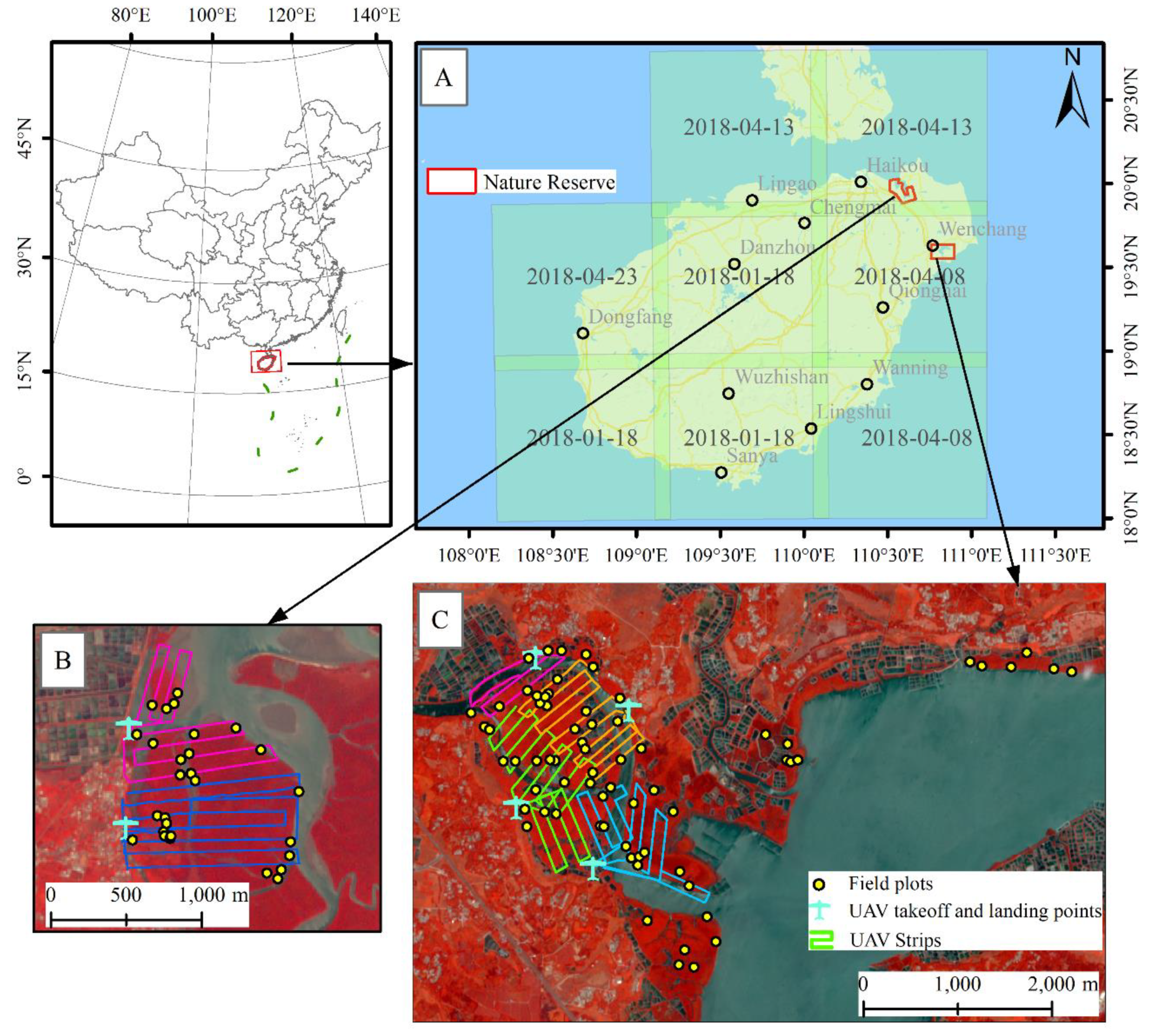
Figure 1.
The location of the study area. (A) Map of Hainan island; the locations and acquisition dates of the Sentinel-2 imagery used in this study are indicated. The field sampling area in (B) Dongzhai National Nature Reserve and (C) Qinglan Provincial Nature Reserve are presented with the false color combination of Sentinel-2 imagery using the near-infrared 1 (R), green (G) and blue (B) bands. The colors of UAV strips are assigned according to the UAV takeoff and landing points.

Figure 2.
Workflow of UAV-LiDAR and Sentinel-2 data acquisition and processing and variable extraction.
Figure 2.
Workflow of UAV-LiDAR and Sentinel-2 data acquisition and processing and variable extraction.

Figure 3.
Schematic graph of the UAV-LiDAR sampling method for height (top graph) and AGB (bottom graph) estimations.
Figure 3.
Schematic graph of the UAV-LiDAR sampling method for height (top graph) and AGB (bottom graph) estimations.

Figure 4.
The OOB error versus the number of variables resulting from running the RF-based backward feature elimination method 20 times. (A) The LiDAR~S2 model for mangrove height estimation; (B) the G~LiDAR model; (C) the model; and (D) the G~S2 model for mangrove AGB estimations. The optimal number of variables is presented in the graph.

Figure 5.
(A) Boxplots of the observed (I) and predicted values (II) for mangrove height (LiDAR~S2) and AGB () models, respectively. (B) Scatterplot of the residual error versus observed height values (LiDAR~S2) (C) Scatterplots of the residual error versus the field-estimated mangrove AGB for the model; (D) Scatterplots of the residual error versus the field-estimated mangrove AGB for the traditional G~S2 model.

Figure 6.
Mangrove height map of Hainan Island at 10 m spatial resolution. (A) Whole Hainan Island, (B) Dongzhai Harbor, (C) Qinglan Harbor, (D) Danzhou Bay, and (E) Meilang Harbor.
Figure 6.
Mangrove height map of Hainan Island at 10 m spatial resolution. (A) Whole Hainan Island, (B) Dongzhai Harbor, (C) Qinglan Harbor, (D) Danzhou Bay, and (E) Meilang Harbor.

Figure 7.
Mangrove aboveground biomass map of Hainan Island at 10 m spatial resolution. (A) Whole Hainan Island, (B) Dongzhai Harbor, (C) Qinglan Harbor, (D) Danzhou Bay, and (E) Meilang Harbor.
Figure 7.
Mangrove aboveground biomass map of Hainan Island at 10 m spatial resolution. (A) Whole Hainan Island, (B) Dongzhai Harbor, (C) Qinglan Harbor, (D) Danzhou Bay, and (E) Meilang Harbor.

Figure 8.
The importance of different variables measured by %IncMSE (the percentage increase in the mean square error) after running the random forest algorithm 100 times: (A) the LiDAR~S2 model for height estimation; (B) the G~LiDAR model and (C) the G~S2 model for AGB estimation.
Figure 8.
The importance of different variables measured by %IncMSE (the percentage increase in the mean square error) after running the random forest algorithm 100 times: (A) the LiDAR~S2 model for height estimation; (B) the G~LiDAR model and (C) the G~S2 model for AGB estimation.

Figure 9.
An illustration of the reforestation plan on Hainan Island: shrimp ponds were converted to mudflats and finally to mangrove forests. This happened in the Qinglan Harbor. The images are from Google Earth.
Figure 9.
An illustration of the reforestation plan on Hainan Island: shrimp ponds were converted to mudflats and finally to mangrove forests. This happened in the Qinglan Harbor. The images are from Google Earth.

Figure 10.
Illustrations of fieldwork challenges in mangrove habitat. This was conducted on Hainan Island: (A) walking barefoot in mangrove habitat; (B) field sampling in an R. stylosa community inundated by the tide; (C) measuring the diameter breast height in an R. apiculata community with dense prop roots at the bottom.

Figure 11.
Illustrations of UAV-LiDAR point cloud profiles of B. sexangula (left), R. stylosa (center), and L. racemosa (right).
Figure 11.
Illustrations of UAV-LiDAR point cloud profiles of B. sexangula (left), R. stylosa (center), and L. racemosa (right).

Table 1.
Summary of the species-specific aboveground biomass allometric equations used in this study. The units of AGB, DBH, and H are kg, cm, and m, respectively.
Table 1.
Summary of the species-specific aboveground biomass allometric equations used in this study. The units of AGB, DBH, and H are kg, cm, and m, respectively.
| Species | Allometric Equation | Country | Reference |
|---|---|---|---|
| A. corniculatum | China | [27] | |
| A. marina1 | China | [28] | |
| B. sexangula | Australia | [29] | |
| C. tagal | Australia | [29] | |
| E. agallocha | Bangladesh | [30] | |
| H. littoralis2 H. tiliaceus2 | Thailand Indonesia | [31] | |
| K. candel | China | [27] | |
| L. racemosa | Guiana, French | [32] | |
| R. apiculata | Malaysia | [33] | |
| R. stylosa | Australia | [29] | |
| S. apetala3 | Thailand Indonesia | [31] | |
| Sonneratia spp.4 | Indonesia | [34] | |
| X. granatum | Australia | [29] |
Table 2.
Confusion matrix and mangrove classification accuracy. OA denotes overall classification accuracy; UA denotes user’s accuracy; PA denotes producer’s accuracy.
Table 2.
Confusion matrix and mangrove classification accuracy. OA denotes overall classification accuracy; UA denotes user’s accuracy; PA denotes producer’s accuracy.
| Mangroves | Non-Mangroves | UA | |
|---|---|---|---|
| mangrove | 193 | 7 | 96.50% |
| non-mangroves | 1 | 199 | 99.50% |
| PA | 99.48% | 96.60% | |
| Kappa: 0.96 | OA: 98.00% |
Table 3.
The selected features from the RF-based backward feature elimination method.
| Model | Number | Selected Features | |
|---|---|---|---|
| Height | LiDAR~S2 | 6 | B2, B11, B12, MDI1, MNDWI, MTCI |
| AGB | G~LiDAR | 11 | CC1.3, CTHK, D01, H05, H10, H80, H95, H90, HIQ, HSD, HVAR |
| 12 | B2, B7, B11, B12, MDI1, MDI2, MCARI, MNDWI, MTCI, NDVIre2, NDVIre3, S2REP | ||
| G~S2 | 14 | B2, B3, B4, B5, B11, CIre1, CIre3, EVI, MDI1, MNDWI, MTCI, NDVIre2, NDVIre1, SR |
Table 4.
Calibration and validation results of the height and AGB models.
| Method | Model | Calibration | Validation | |||
|---|---|---|---|---|---|---|
| R2 | RMSE (%) | R2 | RMSE (%) | |||
| Height | UAV-LiDAR sampling | LiDAR~S2 | 0.66 | 1.99 (27.26%) | 0.67 | 1.90 (26.24%) |
| AGB | UAV-LiDAR sampling | G~LiDAR | 0.80 | 40.54 (28.13%) | 0.78 | 42.29 (29.35%) |
| 0.67 | 41.29 (28.65%) | 0.62 | 50.36 (35.41%) | |||
| Traditional | G~S2 | 0.48 | 64.92 (45.05%) | 0.52 | 56.63 (39.82%) | |
Table 5.
Summaries of the mangrove AGB and height (H) in different districts of Hainan Island.
| Districts | Area(ha) | Total AGB (Mg) | Mean AGB (Mg ha−1) | Min AGB (Mg ha−1) | Max AGB (Mg ha−1) | SD AGB (Mg ha−1) | Mean H (m) | Min H (m) | Max H (m) | SD H (m) | |
|---|---|---|---|---|---|---|---|---|---|---|---|
| 1 | Haikou | 1508.14 | 160,565.38 | 106.47 | 14.00 | 268.20 | 45.22 | 5.93 | 2.03 | 10.75 | 1.91 |
| 2 | Wenchang | 1036.03 | 155,462.22 | 150.06 | 14.59 | 291.24 | 48.17 | 8.23 | 2.10 | 17.11 | 2.30 |
| 3 | Danzhou | 539.49 | 72,331.96 | 134.07 | 15.08 | 258.74 | 30.00 | 7.32 | 2.12 | 15.09 | 1.58 |
| 4 | Chengmai | 224.47 | 30,619.86 | 136.41 | 24.19 | 216.92 | 22.48 | 7.12 | 2.98 | 10.15 | 0.93 |
| 5 | Lingao | 151.39 | 19,265.79 | 127.26 | 18.08 | 221.96 | 30.84 | 6.70 | 2.31 | 9.21 | 1.05 |
| 6 | Sanya | 117.51 | 17,091.89 | 145.45 | 51.19 | 255.15 | 28.32 | 7.17 | 3.09 | 15.30 | 1.93 |
| 7 | Dongfang | 77.26 | 11,998.73 | 155.30 | 59.72 | 222.37 | 18.44 | 8.06 | 3.56 | 10.65 | 0.90 |
| 8 | Lingshui | 25.99 | 3781.29 | 145.49 | 39.16 | 266.72 | 31.22 | 7.56 | 3.21 | 14.45 | 1.74 |
| 9 | Qionghai | 16.74 | 3082.20 | 184.12 | 86.03 | 263.80 | 25.17 | 9.88 | 4.24 | 14.11 | 1.15 |
| SUM | Hainan Island | 3697.02 | 474,199.31 | 128.27 | 14.01 | 291.24 | 45.87 | 6.99 | 2.03 | 17.11 | 2.14 |
© 2019 by the authors. Licensee MDPI, Basel, Switzerland. This article is an open access article distributed under the terms and conditions of the Creative Commons Attribution (CC BY) license (http://creativecommons.org/licenses/by/4.0/).
Share and Cite
MDPI and ACS Style
Wang, D.; Wan, B.; Qiu, P.; Zuo, Z.; Wang, R.; Wu, X. Mapping Height and Aboveground Biomass of Mangrove Forests on Hainan Island Using UAV-LiDAR Sampling. Remote Sens. 2019, 11, 2156. https://doi.org/10.3390/rs11182156
AMA Style
Wang D, Wan B, Qiu P, Zuo Z, Wang R, Wu X. Mapping Height and Aboveground Biomass of Mangrove Forests on Hainan Island Using UAV-LiDAR Sampling. Remote Sensing. 2019; 11(18):2156. https://doi.org/10.3390/rs11182156
Chicago/Turabian StyleWang, Dezhi, Bo Wan, Penghua Qiu, Zejun Zuo, Run Wang, and Xincai Wu. 2019. "Mapping Height and Aboveground Biomass of Mangrove Forests on Hainan Island Using UAV-LiDAR Sampling" Remote Sensing 11, no. 18: 2156. https://doi.org/10.3390/rs11182156
Note that from the first issue of 2016, this journal uses article numbers instead of page numbers. See further details here.