Mathematical Integration of Remotely-Sensed Information into a Crop Modelling Process for Mapping Crop Productivity


1
Department of Statistics, Chonnam National University, Gwangju 61186, Korea
2
Applied Plant Science, Chonnam National University, Gwangju 61186, Korea
3
Satellite Information Center, Korea Aerospace Research Institute, 169-84 Gwahak-ro, Yuseong-gu, Daejeon 34133, Korea
*
Author to whom correspondence should be addressed.
†
Equal contribution to the first authorship goes to this author.
Remote Sens. 2019, 11(18), 2131; https://doi.org/10.3390/rs11182131
Submission received: 26 July 2019
/
Revised: 4 September 2019
/
Accepted: 10 September 2019
/
Published: 13 September 2019
(This article belongs to the Special Issue Smart Data Assimilations, Crop Modelling and Remote Sensing in Agriculture Monitoring)
Abstract
:Remote sensing is a useful technique to determine spatial variations in crop growth while crop modelling can reproduce temporal changes in crop growth. In this study, we formulated a hybrid system of remote sensing and crop modelling based on a random-effect model and the empirical Bayesian approach for parameter estimation. Moreover, the relationship between the reflectance and the leaf area index was incorporated into the statistical model. Plant growth and ground-based canopy reflectance data of paddy rice were measured at three study sites in South Korea. Spatiotemporal vegetation indices were processed using remotely-sensed data from the RapidEye satellite and the Communication Ocean and Meteorological Satellite (COMS). Solar insulation data were obtained from the Meteorological Imager (MI) sensor of the COMS. Reanalysis of air temperature data was collected from the Korea Local Analysis and Prediction System (KLAPS). We report on a statistical hybrid approach of crop modelling and remote sensing and a method to project spatiotemporal crop growth information. Our study results show that the crop growth values predicted using the hybrid scheme were in statistically acceptable agreement with the corresponding measurements. Simulated yields were not significantly different from the measured yields at p = 0.883 in calibration and p = 0.839 in validation, according to two-sample t tests. In a geospatial simulation of yield, no significant difference was found between the simulated and observed mean value at p = 0.392 based on a two-sample t test as well. The fabricated approach allows us to monitor crop growth information and estimate crop-modelling processes using remote sensing data from various platforms and optical sensors with different ground resolutions.
1. Introduction
Satellite-based remote sensing is a useful technique to acquire spatiotemporal data consisting of a large number of pixels, but a relatively small number of temporal data points, from an agricultural field. Remote sensing can provide an inexpensive and non-destructive method from various platforms to collect a vast amount of information from an agricultural field [1]. However, there are two main difficulties related to the practical use of remote sensing data from satellite-aboard sensors in monitoring crop growth. Acquisition of remotely sensed data with a high spatial resolution that is feasible for use is limited, due to dependence on revisiting times, operational schedules, and clear sky conditions in the case of the optical satellite-based remote sensing that is more frequently applied in agriculture. Leaf area index (LAI) is commonly used to describe the canopy growth of a crop, but it cannot be measured directly from remote-sensing data. These contain the reflectances of light spectra across all waveband regions to measure the index of “greenness” of the plant canopy [1]. Meanwhile, appropriate crop growth models can provide temporal descriptions of crop conditions during the growing season, although the accuracy of this information is based on the quality of the input data, and on model design [2]. By effectively combining the advantages of remote sensing and crop modelling, the strengths of each approach may make up for inherent weaknesses in individual strategies [3].
There have been earlier efforts to combine the techniques of crop modelling and remote sensing. Arkin, et al. [4] proposed the concept of a hybrid model able to use Landsat data. This concept was included in grain sorghum growth simulation models, the sorghum growth model with feedback capacity (SORGF) [5] and the grain sorghum crop growth model (SORKAM) [6]. These models allow a parameter affecting leaf expansion rate to be adjusted to improve the agreement between simulated and measured LAI. Barnes, et al. [7] modified a cereal crop simulation model, CERES-Wheat [8] to allow the model to accept observed LAI values and to adjust related parameters in the model as a function of LAI. Similar approaches have been made using the WOrld FOod STudies (WOFORST) model [9] and the Simple and Universal CROp growth Simulator (SUCROS) model [10] to improve the overall model performance [11,12,13]. WOFORST is a simulation model for the quantitative analysis of the growth and production of annual field crops. The SUCROSE model simulates both potential and water-limited growth of a crop. Huang et al. [11] and Zhao, Chen and Shen [12] empirically assimilated satellite-based remote sensing information into the WOFORST crop model to estimate regional wheat yield. The former used images combined from Moderate Resolution Imaging Spectroradiometer (MODIS) data and three Landsat TM images while the latter used MODIS images only. Launay and Guerif [13] also reported an integration scheme of SPOT satellite images into the SUCROS model to advance its performance for spatial application in prediction of sugar beet production. Although these approaches quantitatively calibrate the crop model to the actual field conditions for each application, it needs achieving the same inputs required for the crop models. The minimum input requirements for simulation include climate data, soil property data, cultivar-specific genetic coefficients, and field management data [8]. These requirements can be too much to allow the model to be run for an appropriate time in some cases.
GRAMI [3,14,15] is a crop model that uses remotely sensed data and is designed to simulate gramineous crops, such as wheat, corn, and sorghum, using simple inputs (i.e., weather and remote sensing data). GRAMI includes a within-season calibration method, which allows the model to fit measured LAI values using an iterative numerical procedure. Thus, model parameters and initial conditions can be adjusted based on comparisons between measured and simulated values. The resulting simulated crop growth minimizes the error between simulated leaf areas and values of leaf areas obtained from remote sensing. An advantage of this procedure is the capability to use infrequent observations to calibrate the model. The GRAMI model was further developed and was applied to simulate cotton growth and lint yield under limited irrigation conditions [16,17], as well as geospatial projections of rice productivity [18]. The crop modelling technique formulated in GRAMI was applied to assess and monitor crop conditions and yields at regional scales, using imagery from operational satellites [19,20,21,22,23]. This within-season calibration methodology was also used to estimate evaporation and biomass production [24,25].
The remote sensing data either from airborne or satellite platforms is spatiotemporal data consisting of many pixels but a relatively small number of time points. For example, the reflectance can be obtained from the RapidEye satellite with a ground resolution of 5 m at 800 × 800 pixels five times during a crop-growing season in a monsoonal climate region. A hybrid approach utilizing both remote sensing and crop modelling can fill the temporal gap. Parameters that characterize a crop model are not necessarily constant. However, pixel-by-pixel estimation is not a good choice for studying the spatial variation in the parameters for the following two reasons. First, the model can be unidentifiable when the sample size is smaller than the number of unknown parameters. Second, as illustrated in James and Stein [26] and Efron and Morris [27,28], the pixel-by-pixel estimate is not optimal with respect to the mean-squared loss. An empirical Bayesian method is introduced to overcome the above-mentioned difficulties. Bayesian methods are characterized by the following concepts and procedures. Random variables are used to model all sources of uncertainty in statistical models, e.g., uncertainty due to lack of information. Determination of the prior probability distribution is required to take into account the prior information. Use of Bayes’ formula is sequentially performed, calculating the posterior distribution when more data become available. In Bayesian statistics, the probability can range from 0 to 1. In this paper, a random-effect model is used to describe the location-dependent unknown parameters, and the empirical Bayesian approach is adopted. A random effect is a factor whose levels are considered a random sample from some population, technically considered to have a normal distribution. Moreover, the relationship between reflectance and LAI is incorporated into the statistical model. These models allow us to monitor the crop growth and estimate the crop model using the remote sensing data from various platforms and optical sensors with different ground resolutions. We report a statistical hybrid approach of crop modelling and remote sensing as well as a method to project spatiotemporal crop growth information using paddy rice (Oryza sativa). It is one of the main food crops for more than half of the world’s population, including about 557 million people in Asia.
2. Materials and Methods
2.1. Study Sites
Ground-measured growth and yield and remote sensing data of crop growth were obtained for three separate rice paddy sites: one (field area of ~0.4 km2) site was located at the experimental fields of Chonnam National University (CNU), Gwangju and the other two sites were commercial farm fields (each field area of ~1 km2 at Buan and Gimje), Chonbuk Province, South Korea (Figure 1). The mean annual air temperature and the annual precipitation averaged over the past three decades (1981–2010) are 13.8 °C and 1391 mm year–1 in Gwangju, 13.3 °C and 1313 mm year–1 in Gimje, and 12.6 °C and 1250 mm year–1 in Buan, respectively (Korea Meteorological Administration) [29]. The East Asian monsoon climate is dominant from June to October in these regions, with more than half of the annual precipitation falling during this period.
2.2. Crop Growth Data
Paddy rice growth simulation at the field scale was performed using ground-based remote sensing input data obtained at the CNU site in 2011, 2012, and 2013 and the Buan and Gimje sites in 2014. At the CNU site, 30-day-old rice seedlings (cv. Hopum in 2011, cv. Hwasunchal in 2012, and cv. Unkwang in 2013) were mechanically transplanted in paddy fields on 6 June 2011 (day of year (DOY) 157), 28 May 2012 (DOY 148), and 20 May 2013 (DOY 140). At the Buan and Gimje sites, 30-day-old rice seedlings (cv. Ilmi at Buan and cv. Saenuri and Sindongin at Gimje) were transplanted on 28 May 2014 (DOY 148). Nitrogen (N), phosphate (P), and potassium (K) fertilizers were applied in amounts corresponding to 90 N, 50 P, and 60 K kg·ha–1, respectively.
Data collected were canopy reflectance of plants, using an MSR16R multispectral radiometer (CROPSCAN Inc., Rochester, Minnesota, USA), and LAI using an LI-2200 Plant Canopy Analyser (LI-COR Inc., Lincoln, Nebraska, USA). These data were measured with four replications on DOY 188, 194, 201, 207, 215, 223, 229, 236, 243, 250, 257, and 265 in 2011; on DOY 173, 184, 193, 201, 207, 213, 226, 237, 243, 249, 262, and 276 in 2012; and on DOY 167, 172, 182, 190, 200, 206, 220, 231, and 241 in 2013 at the CNU site. Data at both the Buan and Gimje sites were measured on DOY 165, 177, 195, 203, 223, 238, 258, and 276 in 2014. The yield was estimated by multiplying four yield components, which were measured three times in the sample plots, based on random sampling at maturity. The yield components were panicle number per m2, spikelet number per panicle, percentage of filled grain, and the weight of 1000 grains. Weather data at the CNU site were measured using an automated weather station (WS-GP1, Delta-T Devices, Cambridge, UK). Climate data for simulation for the Buan and Gimje sites were obtained from the Korea meteorological weather stations (https://data.kma.go.kr/cmmn/main.do, accessed on 6 October 2018).
Four vegetation indices (VIs) (Table 1) were calculated using the reflectance data as input for evaluation of the crop model formulated in this study. The four VIs were empirically chosen from structural indices available and effective for the growth determination of plant canopies using wavebands (i.e., 560, 660, and 800 nm) of multispectral optical sensors in most satellites. In these datasets, both VIs and LAI are observable. However, data of only one point is available.
2.3. Remote Sensing Data
We used remote sensing images from two satellites, i.e., the COMS with the medium ground resolution of 500 m and the RapidEye with the high ground resolution of 6.5 m. The COMS developed by the Korea Aerospace Research Institute (KARI) and launched on 27 June 2010, is a geostationary satellite stationed at an altitude of 3600 km above the Earth’s equator and at a longitude of 128.2°E. The COMS loads two typical sensors of the GOCI and the MI (Table 2). The GOCI can observe the Korean landscape eight times a day, with eight spectral wavebands mounted on the system. The primary objectives of the GOCI sensor are: (1) to detect, monitor and forecast short-term biophysical phenomena; (2) to analyse the bio-geochemical variables and the cycles; and (3) to identify information on the yellow dust and land classification. The GOCI was predominantly considered to monitor the ocean phenomena, with a Sea-Viewing Wide Field-of-View Sensor (SeaWiFS) spectral band [34]. However, its high temporal resolution of the observations and vegetation-sensitive spectral wavebands are mostly suitable for land surface-based applications and, more specifically, for monitoring various types of crop information and conditions [23]. In this study, the GOCI is used to determine the cumulative vegetation indices (VIs) in South Korea, since the setup is responsive to vegetation bands (i.e., red and near infrared, NIR).
RapidEye [35] collects 4 million square kilometres of data per day (Table 2). RapidEye satellite images comprise five spectral wavebands (red, green, blue, red edge, and near-infrared) and are provided commercially using three processing levels: “Level 1B” geometrically uncorrected images, “Level 3A” ortho-rectified tile images with radiometric, geometric, and terrain corrections, and “Level 3B” ortho-rectified, bundle-adjusted images that are larger than the Level 3A products [35]. The Gimje and Buan sites were selected, along with the availability of the RapidEye satellite images (Plant Labs, Inc., CA, USA) for 2014, to perform simulations at the regional scale. For the present study, we obtained radiometrically and geometrically corrected Level 3A images, including the Buan and Gimje sites that were acquired on DOY 149 (29 May), 198 (17 July), 221 (9 August), and 256 (13 September) in 2014. These images contained reflectance values with four different wavebands at 11,700 × 7900 pixels with a size of 5 m. The image data were further processed to classify rice paddy field areas using a digitized paddy coverage map from the Korea Ministry of Environment.
Likewise in the model evaluation procedure, four different VIs (Table 1) were determined and used to project spatiotemporal productivity of paddy rice using the developed crop modelling design discussed in the following section.
2.4. Climate Data
The incident solar radiance on the surface (insolation) estimated using the COMS MI and the air temperatures from the Korea local analysis and prediction system (KLAPS) were used to evaluate the updated GRAMI model to simulate crop growth. The insolation data reflected the energy source of photosynthesis in crop canopies. The missions of the MI sensor (Table 2) comprises continuous monitoring of imagery and extracting of meteorological products to allow early detection of severe weather phenomena and to monitor climate change and the atmospheric environment. The MI has been used to estimate the insolation as the infrared channels can be useful for interpreting the complicated cloud effects. In this study, a pixel-based physical model, using instantaneous satellite observations and atmospheric information, was adjusted out of various satellite-based insolation models [36,37,38].
The satellite-based solar insolation from COMS MI was calculated using the Kawamura physical model [39]. This model contains an improved cloud factor, as it considers the visible satellite reflectance and the solar zenith angle instead of the illumination temperature because the passing depth of the cloud is more sensitive to the amount of irradiance attenuation [40]. The physical model used to estimate the insolation is as follows [39,40,41,42]:
where ST, SI, SR, and SA are the total insolation, direct irradiance, diffuse irradiance due to Rayleigh scattering, and the diffuse irradiance due to scattering by aerosols, respectively. These parameters are used for the physical model of the satellite-based solar insolation [43]. The ST, SI, SR, and SA formulations are as follows:
where the symbols used are represented as follows: incident solar constant, S; transmittance due to absorption by ozone, τo [44]; transmittance due to Rayleigh scattering, τR [45]; transmittance due to attenuation by aerosols, τA [46]; absorption of water vapor, αw [44]; ratio of forward to total scattering by aerosols, Fc [47]; single scattering albedo, ωo; solar constant, I [48]; the annual mean Sun-Earth distance, dM; Sun-Earth distance, d; and solar zenith angle, θ, respectively.
In this study, the topographical corrections were not considered because the selected crop type was mostly cultivated on the flat land surface, and it was difficult to topographically validate corrected insolation, without using applicable ground measurements on an inclined plane. Most of the pyranometers in South Korea were deployed on a horizontal plane, according to the World Meteorological Organization (WMO) criteria (Guide to Meteorological Instruments and Methods of Observation WMO-No. 8).
The KLAPS used to get the air temperatures was designed to forecast weather conditions of the Korean peninsula with a pixel resolution of 5 km for 12 hours, up to 24 times a day [49]. The KLAPS produces reanalysed data, with a comparatively high-resolution of 1.5 km based on its analytical scheme, using all the possible measured weather data from the region of interest. The KLAPS also adapts the data assimilation part of the local analysis and prediction system (LAPS) developed by the US National Oceanic and Atmospheric Administration/Forecast Systems Laboratory (NOAA/FSL). It is classified into both data collection and analysis modules. The analytical process is composed of the surface analysis procedures and three-dimensional wind, temperature, humidity, cloud, precipitation, and soil analysis procedures. The further detailed procedure of the KLAPS can be found in Albers et al. [50].
2.5. Formulation of the GRAMI Model
The four processes (Figure 2) involved in simulating daily rice growth are: (1) interception and absorption of the incident solar radiation by the leaves; (2) calculation of growing degree-days (GDD); (3) production of the new dry mass by the leaf canopy; and (4) determination of the LAI partitioning of the new dry mass. The details of these procedures and related equations are described in Appendix A. In this study, we applied the same initial conditions and parameter values determined in the earlier studies (Table A1) [18,21,23].
LAI is a three-dimensional concept, while the reflectance of plants to solar radiation is a two-dimensional concept because it is electronically recorded as a two-dimensional data for the canopies of crops or mostly the top surface of the plants. We presumed that a log-log regression model, with a slope approximately 2/3, could describe the relationship between reflectance and LAI. Based on this theory, the correlations between five VIs (MTVI, NDVI, RDVI, and OSAVI) and LAI were formulated using log-log linear regression models. For each VI, labelled l = 1, 2, 3, 4, and 5, respectively, an empirical model was framed as follows:
where , and ( represent intercept, slope, and error of the linear regression model, respectively.
The evolution of the LAI for each pixel was explained by the GRAMI-rice model, using four parameters (L0, a, b, and c). These parameters were assumed to be generated from the prior distribution , where the transformations:
were used to guarantee that all four parameters (L0, a, b, and c) range between 0 and 1.
We obtained both the regression coefficients and the hyper-parameters from the data collected in previous studies [18,21]. These included both the VIs and the measured LAI values. The parameter was specified using the ‘before-calibration’ values (L0 = 0.2, a = 3.25 × 10⁻¹, b = 1.25 × 10⁻³, and c = 1.25 × 10⁻³). Parameter D is a diagonal matrix with all diagonal elements equivalent to 0.5.
The following numerical procedure was adopted to obtain for each pixel.
- Step 1: For each pixel, set served as the initial guess of .
- Step 2: Define and consider the objective function:
- Step 3: Generate the simulated curve for each pixel from the estimated in Step 2.
- Step 4: Update as the sample means and sample variances of the estimates in Step 2.
2.6. Modelling Spatiotemporal Crop Productivity
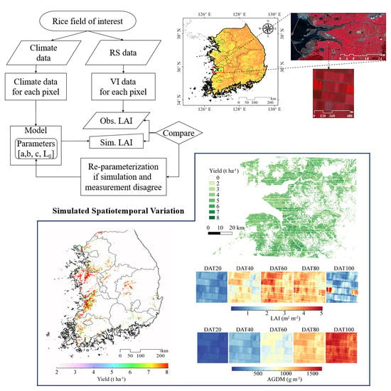
The GRAMI-rice model was formulated to integrate remotely sensed data, allowing agricultural system modellers to reproduce and monitor potential crop production information [18]. The GRAMI model can receive remote sensing data as an input to execute the ‘within-season’ calibration procedure [14]. In this process, simulated crop canopy growth (LAI or VIs) is compared with corresponding measured values to allow agreement with the measurement with a minimal error based on parameterization of specified parameters. Four different coefficients (L0, a, b, and c) are employed in the current model to describe growth processes of rice. Parameter values were obtained through a parameterization process using the Bayesian method with a prior distribution chosen according to the estimates from the previous reports. The relationships between five VIs and LAI were framed using the log-log linear regression models as previously described.
A Crop Information Delivery System (CIDS) was designed earlier as an extended version of the GRAMI-rice model [18] to project pixel-based geospatial crop growth and yield, based on the integration with remote sensing images (Figure 3a). The CIDS employs pixel-based remote sensing data and climate data as the system inputs. The CIDS takes climate data, either from a single weather station or multiple weather stations (pixels) depending on the situation. The GRAMI-rice model is then implemented to simulate crop growth in each pixel using both types of input data.
In the CIDS, the GRAMI model simulates a crop in each pixel using both remote sensing data and climate data as inputs [18]. The new model design was evaluated using paddy field datasets obtained in 2012 at Chonnam National University, Gwangju and in 2014 at Gimje and Gyewha, Chonbuk Province, ROK. The CIDS was then applied using RapidEye satellite images obtained from paddy fields of interest in Chonbuk province, ROK in 2014.
2.7. Statistical Evaluation
Several statistical analytical methods were used to evaluate the reliability of the results. For model evaluation, the mean values of simulated crop yield and LAI were compared with the measured values. A two-sample t-test and two statistical indices of root mean square error, RMSE and model efficiency, ME [53] were applied for the analyses using R software version 3.4.1 [54]. The physical meaning of the ME is that it is a normalized statistic that determines the relative magnitude of the residual variance compared to the observed data variance. ME indicates how well the plot of observed versus simulated data fits the 1:1 line. ME values range from –∞ to 1; the model is more accurate when the value is closer to 1. When values are close to zero, the model predictions are less than or as precise as the observed mean.
3. Results
3.1. Evaluation of Model Performance
The updated GRAMI-rice model performed well in terms of reproducing field conditions of paddy growth in LAI and above-ground dry mass (AGDM). Rice yield could also be determined with reasonable accuracy. For the sake of verification, we used data from CNU, Gwangju from 2011 to 2013 (Figure 4 and Table 3). Simulated seasonal curves for LAI were fit to the corresponding observed values with a model efficiency (ME) of 0.80 and a root mean square error (RMSE) of 0.71 m2 m–2 for cv. Hopum in 2011, an ME of 0.86 and an RMSE of 0.56 m2 m–2 for cv. Hwasunchal in 2012, and an ME of 0.95 and an RMSE of 0.33 m2 m–2 for cv. Unkwang in 2013. Simulated yields agreed well with the observed yields, with an RMSE of 434.9 kg ha–1. According to a two-sample t-test (ɑ = 0.05), the simulated yield (μ = 7,365.7 kg ha–1) was not significantly different (p = 0.883) from the observed yield (μ = 7,190.0 kg ha–1). Validation, using data from Gimje, Chonbuk in 2014 (Figure 5 and Table 3), showed that simulated LAI values agreed with the observed LAI values with an ME of 0.75 and an RMSE of 1.05 m2 m–2 for cv. Sindongjin, an ME of 0.83 and an RMSE of 0.99 m2 m–2 for cv. Saenuri, and an ME of 0.86 and an RMSE of 0.88 m2 m–2 for cv. Ilmi. Simulated yields also agreed with the observed yields, with an RMSE of 426.5 kg ha–1. According to a two-sample t-test (ɑ = 0.05), there was no significant difference (p = 0.839) between the simulated yield (μ = 6937.7 kg ha–1) and the observed yield (μ = 6801.0 kg ha–1).
3.2. Geospatial Projections of Crop Yield and Growth
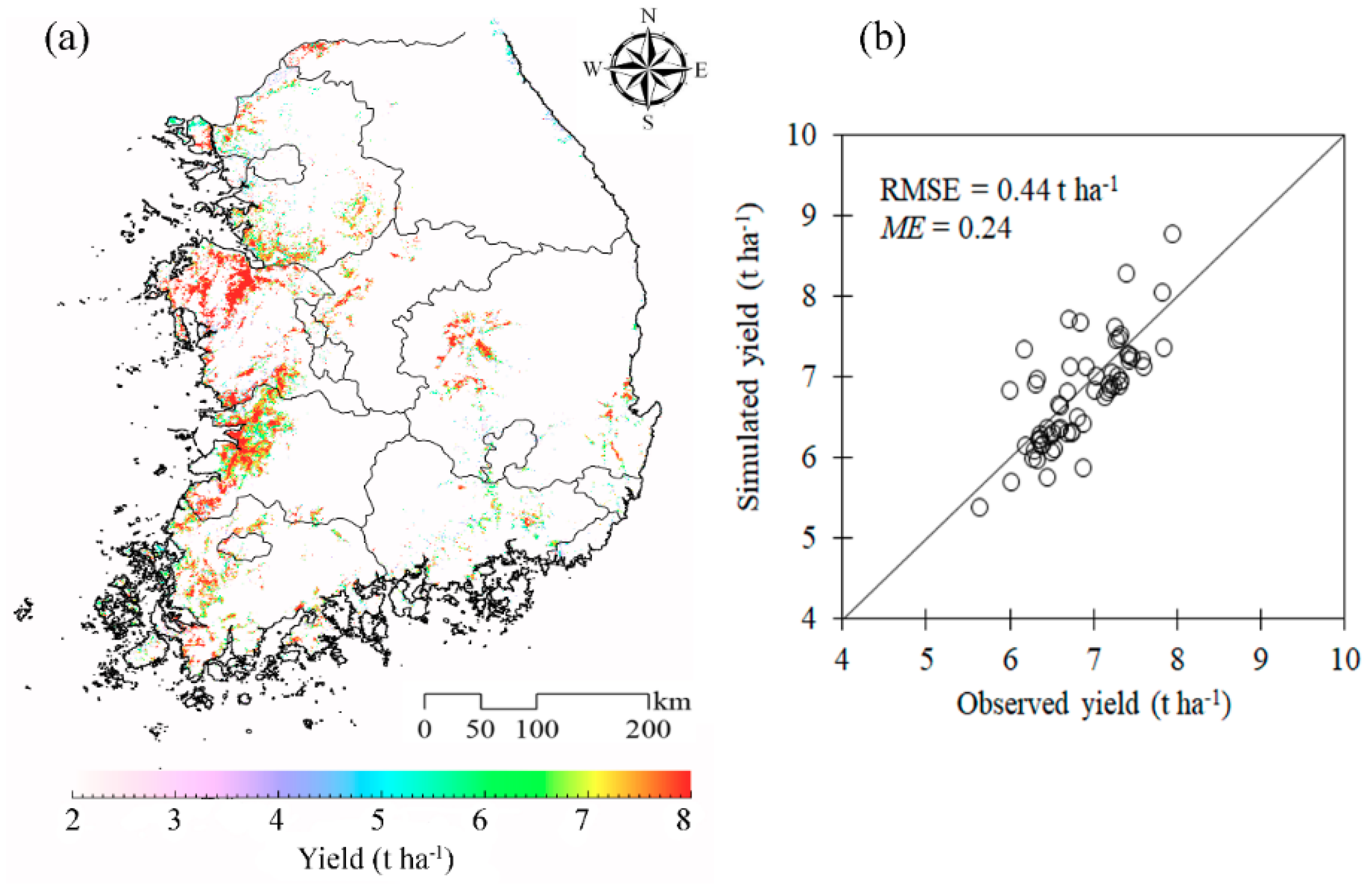
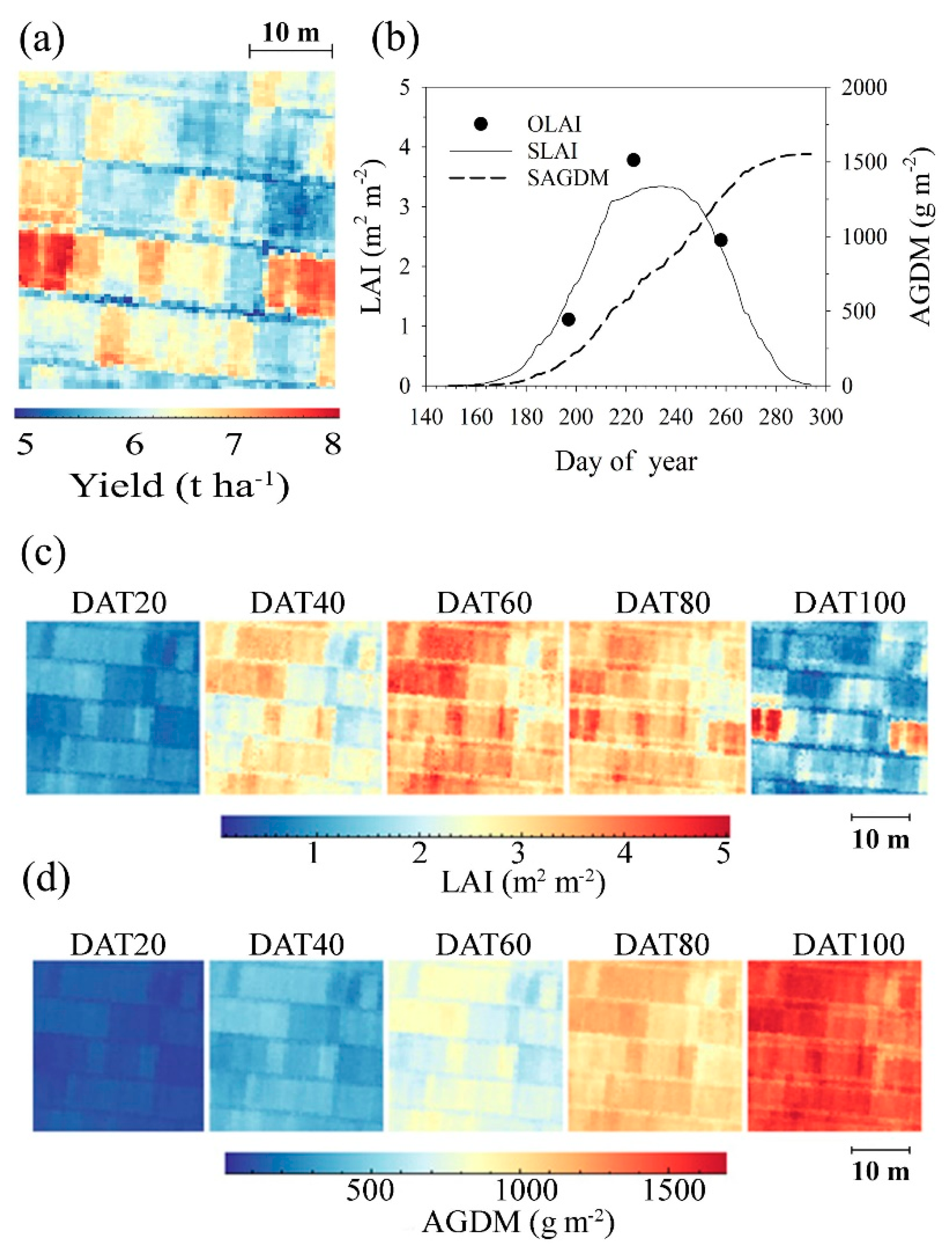
The CIDS well projected geospatial variations in rice yield and growth using satellite images from both the COMS with a medium ground resolution of 500 m (Figure 6) and the RapidEye with a high ground resolution of 5 m (Figure 7). When comparing simulated and observed rice yields (Figure 6b), the simulated mean value (μ = 6.77 t ha–1) was not significantly different (p = 0.392) from the observed mean value (μ = 6.86 t ha–1), according to a two-sample t-test (ɑ = 0.05). These agreed with an RMSE of 0.44 t ha–1 and an ME of 0.24. The CIDS was also designed to project crop productivity information with seasonal patterns, as well as two-dimensional variations on any given day of interest during the crop season. The CIDS produced two-dimensional predictive maps of rice grain yield and growth variables well, with a 5 × 5 m pixel resolution (Figure 8). Predicted grain yields ranged between 4150.6 and 8483.2 kg ha−1, with a mean of 6029.1 kg ha−1. The predicted average value agreed with the field measurement of 6381.9 kg ha−1. Spatiotemporal projections of LAI and AGDM reproduced spatial variations of each growth variable well in the scene during the crop season.
4. Discussion
Our study results presented that the GRAMI-rice model was well integrated with either ground-based remote sensing information or satellite-based remote sensing images with different ground resolutions. The modelling regime reproduced crop growth conditions and yields in significant agreement with the corresponding observations. The current study was dedicated to the statistical hybrid approach of crop modelling and remote sensing, as well as the method to project spatiotemporal crop growth information using remote sensing data from various platforms and optical sensors with different geospatial resolutions. On the other hand, the previous studies using GRAMI-rice were focused on applying for different aspects of crop monitoring, most likely as case studies using images from a specific platform, e.g., an unmanned aerial system, UAS [55] or an optical satellite with either a high ground resolution [21] or a coarse ground resolution [23,56,57].
These simulation results demonstrate that the within-season calibration procedure worked well with the observed LAI inputs incorporated into the model. The updated GRAMI-rice model is theoretically incorporated with a Bayesian method for parameter estimation to facilitate an agreement between simulations and observations based on the POWELL [50] or Quasi-Newton [51] optimisation procedures. The POWELL optimisation routine is carried out for one-point simulation cases while the Quasi-Newton minimiser is performed for two-dimensional simulation cases. We assume that the current parameter estimation method is not only technically unique but also advantageous to assimilate various remote sensing data into crop models that have a strong dependence on input LAI from remotely sensed information. The strong integration of the present GRAMI model with remote sensing data can be a discrete advantage in several ways. First, the present approach requires a simple input requirement, which employs only the existing observations that characterize the environmental circumstances. Earlier versions of the current model also showed the corresponding information [14,16,18]. Second, the optimization method allows the model to advance the simulation performance. Third, the GRAMI model can be assimilated with remotely sensed information from various platforms, e.g., a UAS [55] and operational optical satellites on-board different ground resolution sensors [21,56,57]. Finally, once the model is applied to the satellite-based remote sensing, it is applicable for any region of interest on the Earth’s surface. However, limitations include the inadequate representation of remotely-sensed information as well as partial observations available during the crop-growing season. These can ultimately bring about some level of disagreement between simulations and observations.
While some limitations in the GRAMI model exist including a firm reliance on remotely-sensed data needed to achieve the modelling mentioned above, the requirement of input parameters and variables has significant implications, particularly for inaccessible and data-sparse regions. In such regions, this kind of crop models is practically relevant, since it is almost impossible to monitor or reproduce the crop productivity without using operational satellite-based remote sensing information.
The CIDS is designed to project geospatial information of crop growth and yield using the GRAMI model integrated with remote sensing images from various platforms of remote sensing from an UAS [18,55] to various operational optical satellites with different ground resolutions [21,56,57]. There have been similar practical efforts to assimilate a crop model with satellite images to improve the predictive performance of crop yields [11,12,13]. Meanwhile, the CIDS is unique, in that (1) it is formulated as a whole integrated program to project spatiotemporal variations in crop productivity, as well as (2) the CIDS requires simple input parameters and environmental variables utilizing remote sensing images. One of the critical issues to achieve advanced monitoring of crop productivity information using the system would be to determine a consistent representation of the information on crop canopy reflectance. In this regard, one should acquire stable predefined relationships between LAI and canopy reflectance values or VIs of interest for each crop, based on field experiments. It is essential to determine a reliable classification of crops of interest and to establish spatial variations in different planting dates for each crop well to project practical productivity, especially using coarse resolution satellite images. Dealing with these issues is beyond the scope of this study. It is also essential to extract the endmembers of the mixed pixels in the case of using the coarse resolution satellite images. In the case of the fine resolution satellite images, sparse changes of obtained images can be an issue for simulation, using the previous version of the GRAMI model [18]. The earlier GRAMI model required receipt of an even distribution of several input images during the crop-growing season to achieve dependable simulation outputs. This approach has been optimized in the current version of GRAMI based on the advanced empirical approach, using a predefined relationship between LAI and canopy reflectance values of wavebands or VIs of interest.
5. Conclusion
We present functional coupling of crop modelling and remote sensing using an updated GRAMI-rice model that uses remote sensing data, and a CIDS formulated to simulate geospatial rice growth and yield by adapting the GRAMI-rice model for use in this study. The simulated values of rice growth obtained with the parameterized GRAMI-rice model showed good agreement with the corresponding field measurements. We also presented that GRAMI-rice was successfully incorporated with optical satellite data with different geospatial resolutions. Simulated geographical variations in yield were in reasonable agreement with the corresponding observed variations in yield. Therefore, the current study demonstrates that the GRAMI-rice model can be applied to reproducing rice growth and development conditions and productivity based on the integration with remote sensing data from various platforms such as a UAS and different optical satellites with different ground resolutions. The CIDS was applied to monitoring and mapping of rice growth and yield. The GRAMI-rice model has relatively simple environmental input requirements that can be provided by remote sensing. We assume that the CIDS can be potentially applied to crop growth monitoring and yield mapping efforts for croplands of various geospatial scales, ranging from farm fields to regions of interest because remote sensing data can be obtained from observations of small-size unmanned airborne platforms (drones) and existing satellite sensors.
Author Contributions
Conceptualization: J.K. and C.N.; methodology: V.N.; software: C.N.; validation: J.K., S.J., and J.Y.; formal analysis: S.J.; investigation: V.N.; resources: J.Y.; data curation: S.J.; writing—original draft preparation: J.K.; writing—review and editing: J.K. and J.Y.; visualization: J.K.; supervision: J.K.; project administration: S.J.; funding acquisition: J.K.
Funding
This research was supported by the Basic Science Research Program through the National Research Foundation of Korea (NRF), funded by the Ministry of Education, Science, and Technology (NRF-2015R1D1A1A01057586). Chi Tim NG’s research is supported by a research program of Rural Development Administration, Republic of Korea (project no. PJ01283009).
Acknowledgments
We thank the Korea Institute of Ocean Science and Technology (KIOST) for providing the GOCI data.
Conflicts of Interest
The authors declare no conflict of interest. The funders had no role in the design of the study; in the collection, analyses, or interpretation of data; in the writing of the manuscript; or in the decision to publish the results.
Appendix A
Appendix B

Table A1.
Constant and parameter values used for the GRAMI-rice model [18].
Table A1.
Constant and parameter values used for the GRAMI-rice model [18].
| Symbol | Description | Unit♪ | Value |
|---|---|---|---|
| ε | Radiation use efficiency | g MJ−1 | 3.49 |
| k | Light extinction coefficient | na | 0.6 |
| Ls | Specific leaf area | m2 g−1 | 0.016 |
| Tb | Base temperature | ℃ | 12.0 |
| L0 | Leaf area index at transplant | m2 m−2 | 0.2 |
| pa | The parameter in the leaf allocation function | na | 0.325 |
| pb | The parameter in the leaf allocation function | na | 0.00125 |
| pc | The parameter in the leaf senescence function | na | 0.00125 |
♪ 1 µmol mol−1 is equivalent to 1 ppm.
References
- Jones, H.G.; Vaughan, R.A. Remote Sensing of Vegetation: Principles, Techniques, and Applications; Oxford University Press: New York, NY, USA, 2010. [Google Scholar]
- Maas, S.J. Within-season calibration of modeled wheat growth using remote sensing and field sampling. Agron. J. 1993, 85, 669–672. [Google Scholar] [CrossRef]
- Maas, S.J. GRAMI: A Crop Model Growth Model that Can Use Remotely Sensed Information; USDA-ARS: Washington, DC, USA, 1992; p. 78. [Google Scholar]
- Arkin, G.F.; Ritchie, J.T.; Maas, S.J. A model for calculating light interception by a grain sorghum canopy. Trans. ASAE 1978, 21, 303–308. [Google Scholar] [CrossRef]
- Maas, S.J.; Arkin, G.F. User’s Guide to SORGF: A Dynamic Grain SORGHUM Growth Model with Feedback Capacity; No. 78-1; TAES Program and Model Documentation, Blackland Research Center: Temple, TX, USA, 1978; 107p. [Google Scholar]
- Rosenthal, W.D.; Vanderlip, R.L.; Jackson, B.S.; Arkin, G.F. SORKAM: A Grain Sorghum Crop Growth Model; The Texas agricultural experimental station: Temple, TX, USA, 1989; p. 205. [Google Scholar]
- Barnes, E.M.; Paul, J.; Pinter, J.; Kimball, B.A.; Wall, G.W.; LaMorte, R.L.; Husaker, D.J.; Adamsen, F.; Leavitt, S.; Thompson, T.; et al. Modification of CERES-wheat to accept leaf area index as an input variable. In Proceedings of the ASAE Annual International Meeting, Minneapolis, MN, USA, 14 August 1997; p. 26. [Google Scholar]
- Jones, J.W.; Hoogenboom, G.; Porter, C.H.; Boote, K.J.; Batchelor, W.D.; Hunt, L.; Wilkens, P.W.; Singh, U.; Gijsman, A.J.; Ritchie, J.T. The DSSAT cropping system model. Eur. J. Agron. 2003, 18, 235–265. [Google Scholar] [CrossRef]
- van Diepen, C.A.; Wolf, J.; van Keulen, H.; Rappoldt, C. Wofost: A simulation model of crop production. Soil Use Manag. 1989, 5, 16–24. [Google Scholar] [CrossRef]
- Spitters, C.; Van Keulen, H.; Van Kraalingen, D. A simple and universal crop growth simulator: SUCROS87. In Simulation and Systems Management in Crop Protection; Pudoc: Wageningen, Gelderland, Netherlands, 1989; pp. 147–181. [Google Scholar]
- Huang, J.; Sedano, F.; Huang, Y.; Ma, H.; Li, X.; Liang, S.; Tian, L.; Zhang, X.; Fan, J.; Wu, W. Assimilating a synthetic Kalman filter leaf area index series into the WOFOST model to improve regional winter wheat yield estimation. Agric. For. Meteorol. 2016, 216, 188–202. [Google Scholar] [CrossRef]
- Zhao, Y.; Chen, S.; Shen, S. Assimilating remote sensing information with crop model using Ensemble Kalman Filter for improving LAI monitoring and yield estimation. Ecol. Model. 2013, 270, 30–42. [Google Scholar] [CrossRef]
- Launay, M.; Guerif, M. Assimilating remote sensing data into a crop model to improve predictive performance for spatial applications. Agric. Ecosyst. Environ. 2005, 111, 321–339. [Google Scholar] [CrossRef]
- Maas, S.J. Parameterized model of gramineous crop growth: II. within-season simulation calibration. Agron. J. 1993, 85, 354–358. [Google Scholar] [CrossRef]
- Maas, S.J. Parameterized model of gramineous crop growth: I. leaf area and dry mass simulation. Agron. J. 1993, 85, 348–353. [Google Scholar] [CrossRef]
- Ko, J.; Maas, S.J.; Lascano, R.J.; Wanjura, D. Modification of the GRAMI model for cotton. Agron. J. 2005, 97, 6. [Google Scholar] [CrossRef]
- Ko, J.; Maas, S.J.; Mauget, S.; Piccinni, G.; Wanjura, D. Modeling water-stressed cotton growth using within-season remote sensing data. Agron. J. 2006, 98, 1600–1609. [Google Scholar] [CrossRef]
- Ko, J.; Jeong, S.; Yeom, J.; Kim, H.; Ban, J.-O.; Kim, H.-Y. Simulation and mapping of rice growth and yield based on remote sensing. J. Appl. Remote Sens. 2015, 9, 096067. [Google Scholar] [CrossRef]
- Doraiswamy, P.C.; Hatfield, J.L.; Jackson, T.J.; Akhmedov, B.; Prueger, J.; Stern, A. Crop condition and yield simulations using Landsat and MODIS. Remote Sens. Environ. 2004, 92, 548–559. [Google Scholar] [CrossRef]
- Doraiswamy, P.C.; Sinclair, T.R.; Hollinger, S.; Akhmedov, B.; Stern, A.; Prueger, J. Application of MODIS derived parameters for regional crop yield assessment. Remote Sens. Environ. 2005, 97, 192–202. [Google Scholar] [CrossRef]
- Kim, M.; Ko, J.; Jeong, S.; Yeom, J.-M.; Kim, H.-O. Monitoring canopy growth and grain yield of paddy rice in South Korea by using the GRAMI model and high spatial resolution imagery. Giscience Remote Sens. 2017, 54, 534–551. [Google Scholar] [CrossRef]
- Padilla, F.L.M.; Maas, S.J.; González-Dugo, M.P.; Mansilla, F.; Rajan, N.; Gavilán, P.; Domínguez, J. Monitoring regional wheat yield in Southern Spain using the GRAMI model and satellite imagery. Field Crop. Res. 2012, 130, 145–154. [Google Scholar] [CrossRef]
- Yeom, J.-M.; Ko, J.; Kim, H.-O. Application of GOCI-derived vegetation index profiles to estimation of paddy rice yield using the GRAMI rice model. Comput. Electron. Agric. 2015, 118, 1–8. [Google Scholar] [CrossRef]
- Maas, S.J.; Doraiswamy, P.C. Integration of satellite data and model simulations in a GIS for monitoring regional evaporation and biomass production. In Proceedings of the 3rd International Conference on Integrating GIS and Environmental Modeling, Santa Fe, NM, USA, 21–25 January 1996. [Google Scholar]
- Moran, M.S.; Maas, S.J.; Pinter, P.J., Jr. Combining remote sensing and modeling for estimating surface evaporation and biomass production. Remote Sens. Rev. 1995, 12, 335–353. [Google Scholar] [CrossRef]
- James, W.; Stein, C. Estimation with quadratic loss. In Proceedings of the 4th Berkeley Symposium Mathematical Statistics and Probability, Statistical Laboratory of the University of California, Berkeley, CA, USA, 20 June–30 July 1960; pp. 361–379. [Google Scholar]
- Efron, B.; Morris, C. Data analysis using Stein’s estimator and its generalizations. J. Am. Stat. Assoc. 1975, 70, 311–319. [Google Scholar] [CrossRef]
- Efron, B.; Morris, C. Stein’s paradox in statistics. Sci. Am. 1977, 236, 119–127. [Google Scholar] [CrossRef]
- Korea Meteorological Administration (KMA). Available online: www.kma.go.kr (accessed on 3 September 2019).
- Rouse, J.W., Jr.; Haas, R.H.; Schell, J.A.; Deering, D.W. Monitoring vegetation systems in the Great Plains with ERTS. In Proceedings of the NASA. Goddard Space Flight Center 3d ERTS-1 Symposium, Texas A&M Univ., College Station, TX, USA, 1 January 1974; pp. 309–317. [Google Scholar]
- Roujean, J.-L.; Breon, F.-M. Estimating PAR absorbed by vegetation from bidirectional reflectance measurements. Remote Sens. Environ. 1995, 51, 375–384. [Google Scholar] [CrossRef]
- Rondeaux, G.; Steven, M.; Baret, F. Optimization of soil-adjusted vegetation indices. Remote Sens. Environ. 1996, 55, 95–107. [Google Scholar] [CrossRef]
- Haboudane, D.; Miller, J.R.; Pattey, E.; Zarco-Tejada, P.J.; Strachan, I.B. Hyperspectral vegetation indices and novel algorithms for predicting green LAI of crop canopies: Modeling and validation in the context of precision agriculture. Remote Sens. Environ. 2004, 90, 337–352. [Google Scholar] [CrossRef]
- Wang, M. A Sensitivity Study of the SeaWiFS Atmospheric Correction Algorithm: Effects of Spectral Band Variations. Remote Sens. Environ. 1999, 67, 348–359. [Google Scholar] [CrossRef]
- Tyc, G.; Tulip, J.; Schulten, D.; Krischke, M.; Oxfort, M. The RapidEye mission design. Acta Astronaut. 2005, 56, 213–219. [Google Scholar] [CrossRef]
- Nunez, M. The development of a satellite-based insolation model for the tropical western Pacific Ocean. Int. J. Climatol. 1993, 13, 607–627. [Google Scholar] [CrossRef]
- Otkin, J.A.; Anderson, M.C.; Mecikalski, J.R.; Diak, G.R. Validation of GOES-Based Insolation Estimates Using Data from the U.S. Climate Reference Network. J. Hydrometeorol. 2005, 6, 460–475. [Google Scholar] [CrossRef] [Green Version]
- Pinker, R.; Laszlo, I. Modeling surface solar irradiance for satellite applications on a global scale. J. Appl. Meteorol. 1992, 31, 194–211. [Google Scholar] [CrossRef]
- Kawamura, H.; Tanahashi, S.; Takahashi, T. Estimation of insolation over the Pacific Ocean off the Sanriku coast. J. Oceanogr. 1998, 54, 457–464. [Google Scholar] [CrossRef]
- Yeom, J.-M.; Han, K.-S.; Kim, J.-J. Evaluation on penetration rate of cloud for incoming solar radiation using geostationary satellite data. Asia Pac. J. Atmos. Sci. 2012, 48, 115–123. [Google Scholar] [CrossRef]
- Kawai, Y.; Kawamura, H. Validation and Improvement of Satellite-Derived Surface Solar Radiation over the Northwestern Pacific Ocean. J. Oceanogr. 2005, 61, 79–89. [Google Scholar] [CrossRef] [Green Version]
- Tanahashi, S.; Kawamura, H.; Matsuura, T.; Takahashi, T.; Yusa, H. A system to distribute satellite incident solar radiation in real-time. Remote Sens. Environ. 2001, 75, 412–422. [Google Scholar] [CrossRef]
- Yeom, J.-M.; Seo, Y.-K.; Kim, D.-S.; Han, K.-S. Solar Radiation Received by Slopes Using COMS Imagery, a Physically Based Radiation Model, and GLOBE. J. Sens. 2016, 2016, 1–15. [Google Scholar] [CrossRef] [Green Version]
- Lacis, A.A.; Hansen, J. A Parameterization for the Absorption of Solar Radiation in the Earth’s Atmosphere. J. Atmos. Sci. 1974, 31, 118–133. [Google Scholar] [CrossRef]
- Kizu, S. A Study on Thermal Response of Ocean Surface Layer to Solar Radiation Using Satellite Sensing; Tohoku University: Sendai, Japan, 1995. [Google Scholar]
- Frouin, R.; Lingner, D.W.; Gautier, C.; Baker, K.S.; Smith, R.C. A simple analytical formula to compute clear sky total and photosynthetically available solar irradiance at the ocean surface. J. Geophys. Res. Ocean. 1989, 94, 9731–9742. [Google Scholar] [CrossRef]
- Robinson, G. Absorption of solar radiation by atmospheric aerosol, as revealed by measurements at the ground. Arch. Für Meteorol. Geophys. Und Bioklimatol. Ser. B 1962, 12, 19–40. [Google Scholar] [CrossRef]
- Fröhlich, C.; Brusa, R.W. Solar radiation and its variation in time. Sol. Phys. 1981, 74, 209–215. [Google Scholar] [CrossRef]
- Kim, Y.; Park, O.; Hwang, S. Realtime operation of the Korea Local Analysis and prediction system at METRI. Asia Pac. J. Atmos. Sci. 2002, 38, 1–10. [Google Scholar]
- Albers, S.C.; McGinley, J.A.; Birkenheuer, D.L.; Smart, J.R. The Local Analysis and Prediction System (LAPS): Analyses of Clouds, Precipitation, and Temperature. Weather Forecast. 1996, 11, 273–287. [Google Scholar] [CrossRef] [Green Version]
- Press, W.H.; Teukolsky, S.A.; Vetterling, W.T.; Flannery, B.P. Numerical Recipes: The Art of Scientific Computing; Cambridge University Press: New York, NY, USA, 1992. [Google Scholar]
- Nash, J.C. Compact Numerical Methods for Computers: Linear Algebra and Function Minimisation; CRC Press: Boca Raton, FL, USA; Adam Hilger: New York, NY, USA, 1990. [Google Scholar]
- Nash, J.E.; Sutcliffe, J.V. River flow forecasting through conceptual models part I—A discussion of principles. J. Hydrol. 1970, 10, 282–290. [Google Scholar] [CrossRef]
- R: The R project for statistical computing. Available online: https://www.r-project.org/ (accessed on 25 July 2019).
- Jeong, S.; Ko, J.; Choi, J.; Xue, W.; Yeom, J.-M. Application of an unmanned aerial system for monitoring paddy productivity using the GRAMI-rice model. Int. J. Remote Sens. 2018, 39, 2441–2462. [Google Scholar] [CrossRef]
- Jeong, S.; Ko, J.; Yeom, J.-M. Nationwide Projection of Rice Yield Using a Crop Model Integrated with Geostationary Satellite Imagery: A Case Study in South Korea. Remote Sens. 2018, 10, 1665. [Google Scholar] [CrossRef]
- Yeom, J.-M.; Jeong, S.; Jeong, G.; Ng, C.T.; Deo, R.C.; Ko, J. Monitoring paddy productivity in North Korea employing geostationary satellite images integrated with GRAMI-rice model. Sci. Rep. 2018, 8, 16121. [Google Scholar] [CrossRef] [PubMed]
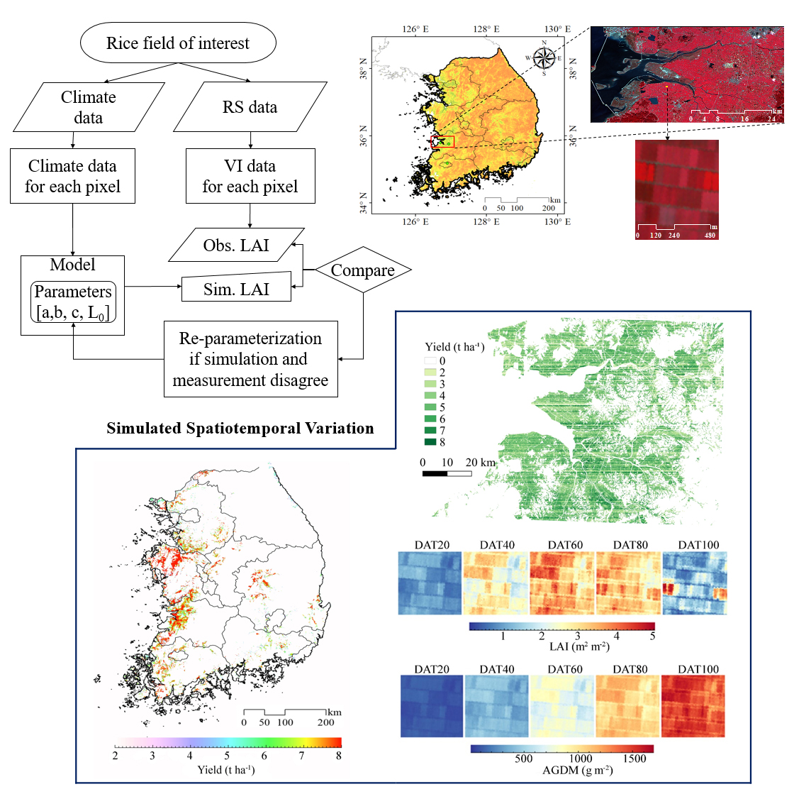
Figure 1.
A shape map of South Korea and three study sites at Buan (top left circle) and Gimje (top right circle), Chonbuk and at Chonnam National University (CNU) in Gwangju (bottom circle), respectively (a) and a pseudo-coloured RapidEye satellite image (b) and a subset imagery (c) taken on 13 September 2014. The map (a) was produced using ArcGIS (ESRI, Inc., Redlands, CA, USA) and the RapidEye images were reproduced using ENVI (Harris Geospatial Solutions, Inc., Broomfield, CO, USA).

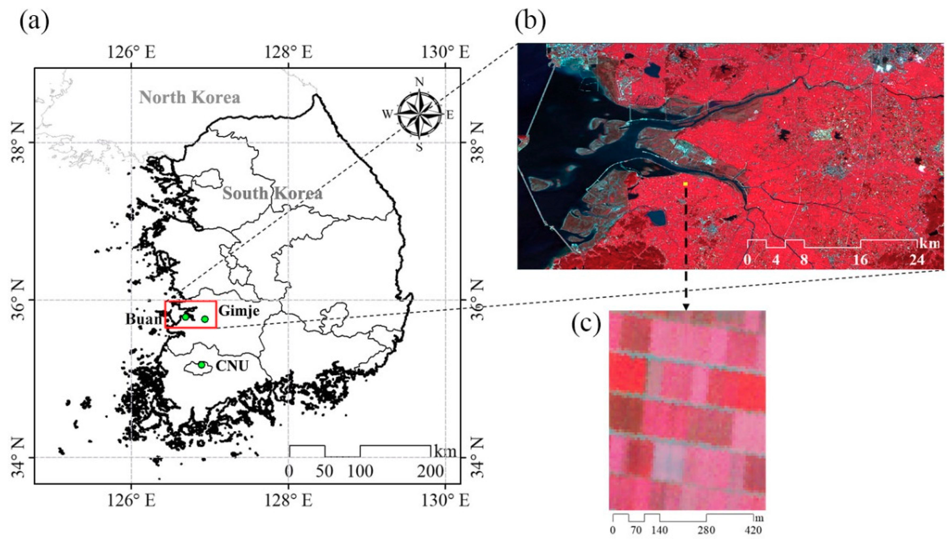
Figure 2.
Schematic diagram of a daily simulation process of crop growth. LAI = leaf area index; PAR = photosynthetic active radiation.
Figure 2.
Schematic diagram of a daily simulation process of crop growth. LAI = leaf area index; PAR = photosynthetic active radiation.

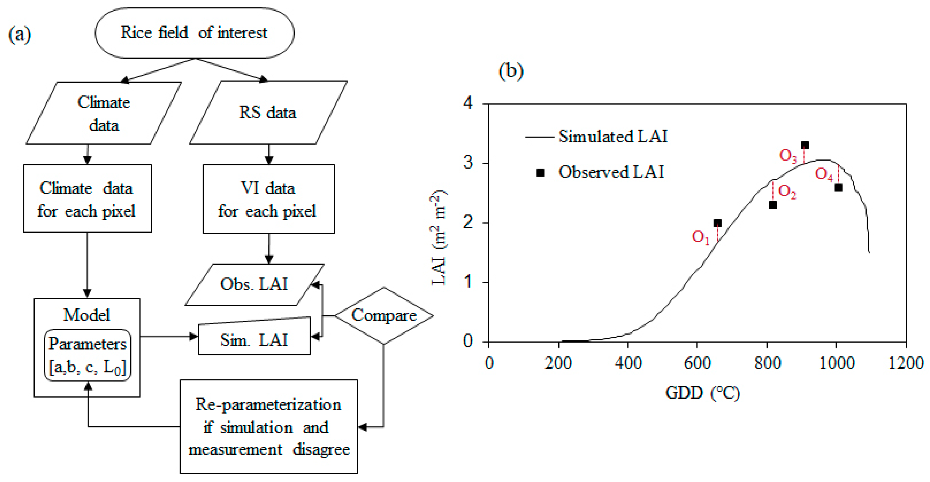
Figure 3.
Diagram of the integrated crop modelling system to project spatiotemporal crop productions using the GRAMI model (a) and observed (O) and simulated leaf area index (LAI) being matched with a minimal error using the within-season calibration (b). GDD = growing degree day; VI = vegetation index.

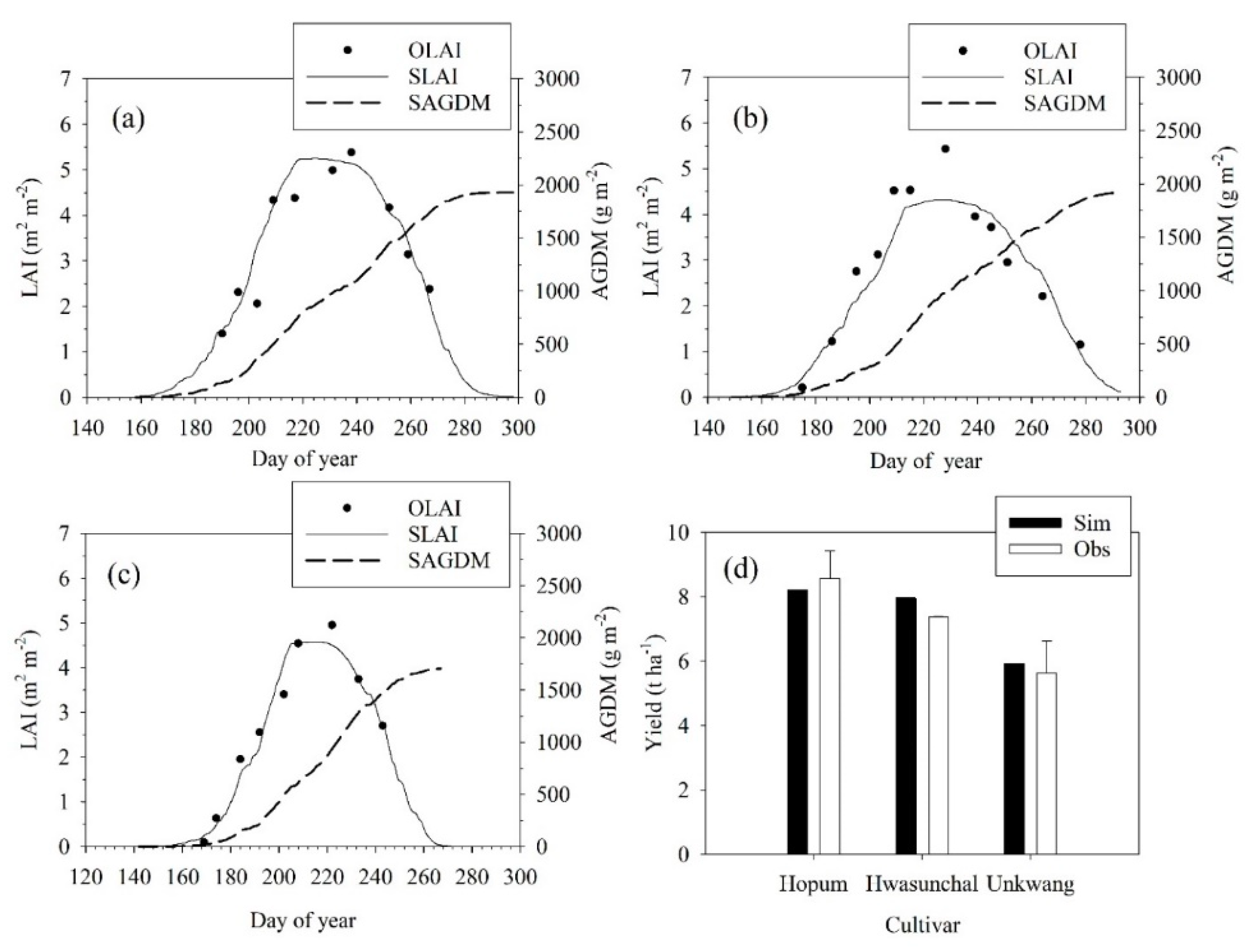
Figure 4.
Simulated (S) and observed (O) leaf area index (LAI) and simulated above ground dry mass (SAGDM) of Hopum in 2001 (a), Hwasunchal in 2012 (b), and Unkwang in 2013 (c), and a comparison between simulated (Sim) and observed (Obs) yields (d) at Chonnam National University, Gwangju, S. Korea for model verification.

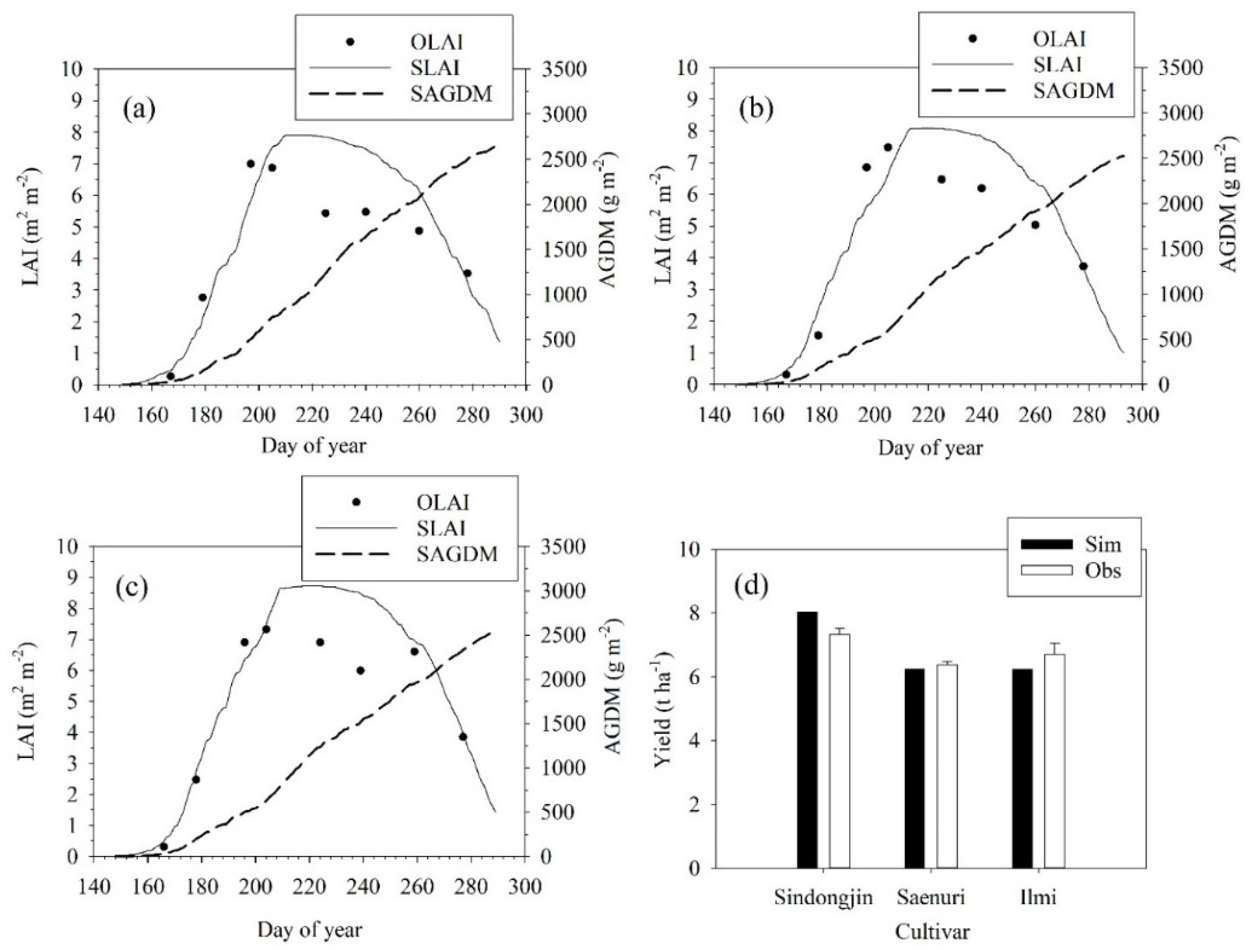
Figure 5.
Simulated (S) and observed (O) leaf area index (LAI) and simulated above ground dry mass (SAGDM) of Sindongin (a), Saenuri (b), and Ilmi (c), and comparison between simulated (Sim) and observed (Obs) yields (d) at Buan and Gimje, Chonbuk, S. Korea in 2014 for model validation.
Figure 5.
Simulated (S) and observed (O) leaf area index (LAI) and simulated above ground dry mass (SAGDM) of Sindongin (a), Saenuri (b), and Ilmi (c), and comparison between simulated (Sim) and observed (Obs) yields (d) at Buan and Gimje, Chonbuk, S. Korea in 2014 for model validation.

Figure 6.
Simulated regional variation in rice yield in South Korea (a) and simulated mean rice yields in comparison with the observed mean rice yields in 62 administrative districts of the country, representing more than 5,000 ha of the paddy areas (b) in 2014. The yield data were simulated using Communication Ocean and Meteorological Satellite (COMS) imageries with a 500-m ground resolution.

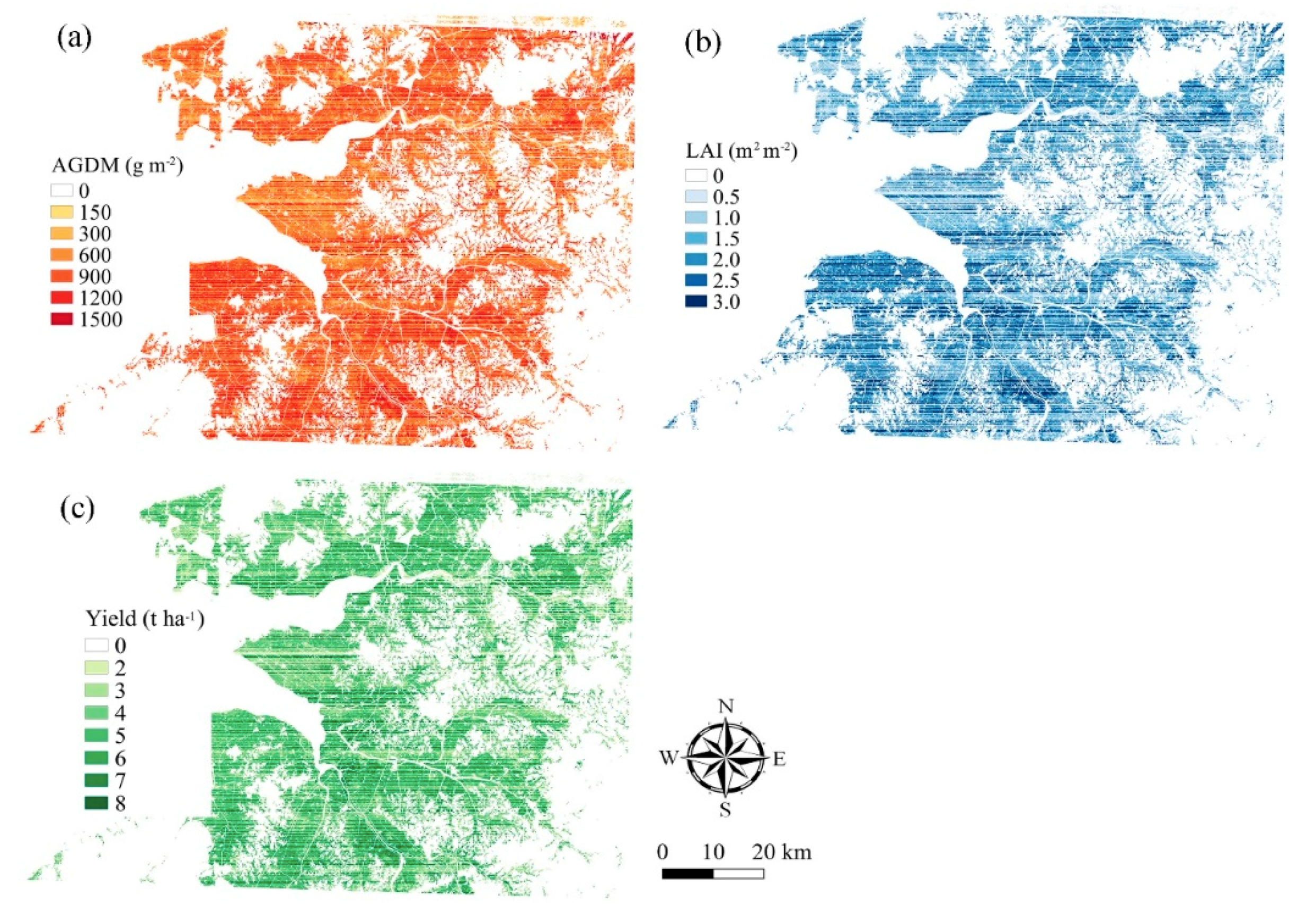
Figure 7.
Simulated regional variations in above ground dry mass, AGDM (a) and leaf area index, LAI (b) at 100 days after transplanting and yield (c) of rice in Gimje in 2014. The data were simulated using RapidEye satellite imageries with a 5-m ground resolution.
Figure 7.
Simulated regional variations in above ground dry mass, AGDM (a) and leaf area index, LAI (b) at 100 days after transplanting and yield (c) of rice in Gimje in 2014. The data were simulated using RapidEye satellite imageries with a 5-m ground resolution.

Figure 8.
Simulated geospatial variation in paddy yield (a), simulated (S) and observed (O), temporal variations in leaf area index (LAI) and above ground dry mass (AGDM) (b), and spatiotemporal variations in LAI (c) and AGDM (d) at 20, 40, 60, 80, and 100 days after transplanting (DAT). The data were simulated using RapidEye satellite imageries with a 5-m ground resolution. .

Table 1.
Vegetation indices used for rice growth phenological stage monitoring and leaf area index estimation.
Table 1.
Vegetation indices used for rice growth phenological stage monitoring and leaf area index estimation.
| Vegetation Index♩ | Equation♪ |
|---|---|
| NDVI [30] | |
| RDVI [31] | |
| OSAVI [32] | |
| MTVI1 [33] |
♩ NDVI = Normalized Difference Vegetation Index, RDVI = Re-normalized Difference Vegetation Index, OSAVI = Optimized Soil-Adjusted Vegetation Index, and MTVI = Modified Triangular Vegetation Index. ♪ R800, R660, and R560 represent the reflectance values of each waveband (800 nm, 660 nm, and 560 nm).
Table 2.
Detailed characteristics of the Geostationary Ocean Colour Imager (GOCI) and the Meteorological Imager (MI) sensors of the Communication Ocean and Meteorological Satellite (COMS) as well as the Multispectral Push-broom Imager (MPI) of the RapidEye satellite.
Table 2.
Detailed characteristics of the Geostationary Ocean Colour Imager (GOCI) and the Meteorological Imager (MI) sensors of the Communication Ocean and Meteorological Satellite (COMS) as well as the Multispectral Push-broom Imager (MPI) of the RapidEye satellite.
| Satellite | Sensor and Orbit Type (Altitude) | Channel | Wavelength (µm) | GSD (km) | IFOV (μrad) |
|---|---|---|---|---|---|
| COMS | GOCI, Geo-synchronous (36,000 km) | B1 | 0.40–0.42 | 0.5 | 28 |
| B2 | 0.43–0.45 | 0.5 | 28 | ||
| B3 | 0.48–0.50 | 0.5 | 28 | ||
| B4 | 0.55–0.57 | 0.5 | 28 | ||
| B5 | 0.65–0.67 | 0.5 | 28 | ||
| B6 | 0.68–0.69 | 0.5 | 28 | ||
| B7 | 0.74–0.76 | 0.5 | 28 | ||
| B8 | 0.85–0.89 | 0.5 | 28 | ||
| MI, Geo-synchronous (36,000 km) | VIS | 0.55–0.80 | 1 | 28 | |
| SWIR | 3.50–4.00 | 4 | 112 | ||
| WV | 6.50–7.00 | 4 | 112 | ||
| IR1 | 10.30–11.30 | 4 | 112 | ||
| IR2 | 11.50–12.50 | 4 | 112 | ||
| RapidEye | MPI, sun-synchronous (630 km) | Blue | 0.44–0.51 | 6.5 × 10⁻³ | 20 |
| Green | 0.52–0.59 | 6.5 × 10⁻³ | 20 | ||
| Red | 0.63–0.685 | 6.5 × 10⁻³ | 20 | ||
| Red edge | 0.69–0.73 | 6.5 × 10⁻³ | 20 | ||
| NIR | 0.76–0.85 | 6.5 × 10⁻³ | 20 |
B1 to B6 = visible, B7 and B8 = near infrared, VIS = visible, SWIR = shortwave infrared, WV = water vapor, IR1 = infrared 1, IR2 = infrared 2, and NIR = near-infrared. GSD = ground sampling distance. IFOV = instantaneous field of view.
Table 3.
Comparisons between simulated and observed mean leaf area index (LAI) of paddy for model calibration at Chonnam National University (CNU), Gwangju and for model validation at Buan and Gimje, Chonbuk in South Korea. Comparison statistics applied were root mean square error (RMSE) and model efficiency (ME).
| Division | Year | Cultivar | Simulation | Observation§ | RMSE | ME |
|---|---|---|---|---|---|---|
| ------------------ m2 m–2 ------------------ | ||||||
| Gwangju | 2011 | Hopum | 3.93 | 3.84 | 0.71 | 0.80 |
| 2012 | Hwasunchal | 2.98 | 2.84 | 0.56 | 0.86 | |
| 2013 | Unkwang | 2.73 | 2.69 | 0.33 | 0.95 | |
| Chonbuk | 2014 | Sindongjin | 4.52 | 4.57 | 1.05 | 0.75 |
| 2014 | Saenuri | 4.70 | 4.62 | 0.99 | 0.84 | |
| 2014 | Ilmi | 5.04 | 5.10 | 0.88 | 0.86 | |
§ Observation was based on the GRAMI model projections using four vegetation indices (VIs), i.e., normalized difference vegetation index (NDVI), re-normalized difference vegetation index (RDVI), modified triangular vegetation index (MTVI), and optimized soil adjusted vegetation index (OSAVI).
© 2019 by the authors. Licensee MDPI, Basel, Switzerland. This article is an open access article distributed under the terms and conditions of the Creative Commons Attribution (CC BY) license (http://creativecommons.org/licenses/by/4.0/).
Share and Cite
MDPI and ACS Style
Nguyen, V.C.; Jeong, S.; Ko, J.; Ng, C.T.; Yeom, J. Mathematical Integration of Remotely-Sensed Information into a Crop Modelling Process for Mapping Crop Productivity. Remote Sens. 2019, 11, 2131. https://doi.org/10.3390/rs11182131
AMA Style
Nguyen VC, Jeong S, Ko J, Ng CT, Yeom J. Mathematical Integration of Remotely-Sensed Information into a Crop Modelling Process for Mapping Crop Productivity. Remote Sensing. 2019; 11(18):2131. https://doi.org/10.3390/rs11182131
Chicago/Turabian StyleNguyen, Van Cuong, Seungtaek Jeong, Jonghan Ko, Chi Tim Ng, and Jongmin Yeom. 2019. "Mathematical Integration of Remotely-Sensed Information into a Crop Modelling Process for Mapping Crop Productivity" Remote Sensing 11, no. 18: 2131. https://doi.org/10.3390/rs11182131
Note that from the first issue of 2016, this journal uses article numbers instead of page numbers. See further details here.